Showing preview only (900K chars total). Download the full file or copy to clipboard to get everything.
Repository: JoinQuant/jqfactor_analyzer
Branch: master
Commit: 69e677dc0dd9
Files: 33
Total size: 23.5 MB
Directory structure:
gitextract_zj34mbsw/

├── .gitignore
├── LICENSE
├── MANiFEST.in
├── README.md
├── docs/
│   └── API文档.md
├── jqfactor_analyzer/
│   ├── __init__.py
│   ├── analyze.py
│   ├── attribution.py
│   ├── compat.py
│   ├── config.json
│   ├── data.py
│   ├── exceptions.py
│   ├── factor_cache.py
│   ├── performance.py
│   ├── plot_utils.py
│   ├── plotting.py
│   ├── prepare.py
│   ├── preprocess.py
│   ├── sample.py
│   ├── sample_data/
│   │   ├── VOL5.csv
│   │   ├── index_weight_info.csv
│   │   └── weight_info.csv
│   ├── utils.py
│   ├── version.py
│   └── when.py
├── requirements.txt
├── setup.cfg
├── setup.py
└── tests/
    ├── __init__.py
    ├── test_attribution.py
    ├── test_data.py
    ├── test_performance.py
    └── test_prepare.py
================================================
FILE CONTENTS
================================================
================================================
FILE: .gitignore
================================================
# Byte-compiled / optimized / DLL files
__pycache__/
*.py[cod]
*$py.class
# C extensions
*.so
# Distribution / packaging
.Python
build/
develop-eggs/
dist/
downloads/
eggs/
.eggs/
lib/
lib64/
parts/
sdist/
var/
wheels/
*.egg-info/
.installed.cfg
*.egg
MANIFEST
# PyInstaller
# Usually these files are written by a python script from a template
# before PyInstaller builds the exe, so as to inject date/other infos into it.
*.manifest
*.spec
# Installer logs
pip-log.txt
pip-delete-this-directory.txt
# Unit test / coverage reports
htmlcov/
.tox/
.coverage
.coverage.*
.cache
nosetests.xml
coverage.xml
*.cover
.hypothesis/
.pytest_cache/
# Translations
*.mo
*.pot
# Django stuff:
*.log
local_settings.py
db.sqlite3
# Flask stuff:
instance/
.webassets-cache
# Scrapy stuff:
.scrapy
# Sphinx documentation
docs/_build/
# PyBuilder
target/
# Jupyter Notebook
.ipynb_checkpoints
# pyenv
.python-version
# celery beat schedule file
celerybeat-schedule
# SageMath parsed files
*.sage.py
# Environments
.env
.venv
env/
venv/
ENV/
env.bak/
venv.bak/
# Spyder project settings
.spyderproject
.spyproject
# Rope project settings
.ropeproject
# mkdocs documentation
/site
# mypy
.mypy_cache/
================================================
FILE: LICENSE
================================================
MIT License
Copyright (c) 2019 JoinQuant
Permission is hereby granted, free of charge, to any person obtaining a copy
of this software and associated documentation files (the "Software"), to deal
in the Software without restriction, including without limitation the rights
to use, copy, modify, merge, publish, distribute, sublicense, and/or sell
copies of the Software, and to permit persons to whom the Software is
furnished to do so, subject to the following conditions:
The above copyright notice and this permission notice shall be included in all
copies or substantial portions of the Software.
THE SOFTWARE IS PROVIDED "AS IS", WITHOUT WARRANTY OF ANY KIND, EXPRESS OR
IMPLIED, INCLUDING BUT NOT LIMITED TO THE WARRANTIES OF MERCHANTABILITY,
FITNESS FOR A PARTICULAR PURPOSE AND NONINFRINGEMENT. IN NO EVENT SHALL THE
AUTHORS OR COPYRIGHT HOLDERS BE LIABLE FOR ANY CLAIM, DAMAGES OR OTHER
LIABILITY, WHETHER IN AN ACTION OF CONTRACT, TORT OR OTHERWISE, ARISING FROM,
OUT OF OR IN CONNECTION WITH THE SOFTWARE OR THE USE OR OTHER DEALINGS IN THE
SOFTWARE.
================================================
FILE: MANiFEST.in
================================================
include LICENSE
include *.txt
include jqfactor_analyzer/sample_data/*.csv
include jqfactor_analyzer/config.json
================================================
FILE: README.md
================================================
# jqfactor_analyzer
jqfactor_analyzer 是提供给用户配合 jqdatasdk 进行归因分析,因子数据缓存及单因子分析的开源工具。
### 安装
```pip install jqfactor_analyzer```
### 升级
```pip install -U jqfactor_analyzer```
### 具体使用方法
**详细用法请查看[API文档](https://github.com/JoinQuant/jqfactor_analyzer/blob/master/docs/API%E6%96%87%E6%A1%A3.md)**
## 归因分析使用示例
### 风格模型的基本概念
归因分析旨在通过对历史投资组合的收益进行分解,明确指出各个收益来源对组合的业绩贡献,能够更好地理解组合的表现是否符合预期,以及是否存在某一风格/行业暴露过高的风险。
多因子风险模型的基础理论认为,股票的收益是由一些共同的因子 (风格,行业和国家因子) 来驱动的,不能被这些因子解释的部分被称为股票的 “特异收益”, 而每只股票的特异收益之间是互不相关的。
(1) 风格因子,即影响股票收益的风格因素,如市值、成长、杠杆等。
(2) 行业因子,不同行业在不同时期可能优于或者差于其他行业,同一行业内的股票往往涨跌具有较强的关联性。
(3) 国家因子,表示股票市场整体涨落对投资组合的收益影响,对于任意投资组合,若他们投资的都是同一市场则其承担的国家因子和收益是相同的。
(4) 特异收益,即无法被多因子风险模型解释的部分,也就是影响个股收益的特殊因素,如公司经营能力、决策等。
根据上述多因子风险模型,股票的收益可以表达为 :
$$
R_i = \underbrace{1 \cdot f_c} _{\text{国家因子收益}} + \underbrace{\sum _{j=1}^{S} f _j^{style} \cdot X _{ij}^{style}} _{\text{风格因子收益}} + \underbrace{\sum _{j=1}^{I} f _j^{industry} \cdot X _{ij}^{industry}} _{\text{行业因子收益}} + \underbrace{u _i} _{\text{个股特异收益}}
$$
此公式可简化为:
$$
R_i = \underbrace{\sum_{j=1}^{K} f_j \cdot X_{ij}}_{\text{第 j 个因子 (含国家,风格和行业,总数为 K) 获得的收益}} + \underbrace{u_i} _{\text{个股特异收益}}
$$
其中:
- $R_i$ 是第 $i$ 只股票的收益
- $f_c$ 是国家因子的回报率
- $S$ 和 $I$ 分别是风格和行业因子的数量
- $f_j^{style}$ 是第 $j$ 个风格因子的回报率, $f_j^{industry}$ 是第 $j$ 个行业因子的回报率
- $X_{ij}^{style}$ 是第 $i$ 只股票在第 $j$ 个风格因子上的暴露, $X_{ij}^{industry}$ 是第 $i$ 只股票在第 $j$ 个行业因子上的暴露,因子暴露又称因子载荷/因子值 (通过<span style="color:red;">`jqdatasdk.get_factor_values`</span>可获取风格因子暴露及行业暴露哑变量)
- $u_i$ 是残差项,表示无法通过模型解释的部分 (即特异收益率)
根据上述公式,对市场上的股票 (一般采用中证全指作为股票池) 使用对数市值加权在横截面上进行加权最小二乘回归,可得到 :
- $f_j$ : 风格/行业因子和国家因子的回报率 , 通过 <span style="color:red;">`jqdatasdk.get_factor_style_returns`</span> 获取
- $u_i$ : 回归残差 (无法被模型解释的部分,即特异收益率), 通过<span style="color:red;"> `jqdatasdk.get_factor_specific_returns` </span>获取
### 使用上述已提供的数据进行归因分析 :
现已知你的投资组合 P 由权重 $w_n$ 构成,则投资组合第 j 个因子的暴露可表示为 :
$$
X^P_j = \sum_{i=1}^{n} w_i X_{ij}
$$
- $X^P_j$ 可通过 <span style="color:red;">`jqfactor_analyzer.AttributionAnalysis().exposure_portfolio` </span>获取
投资组合在第 j 个因子上获取到的收益率可以表示为 :
$$
R^P_j = X^P_j \cdot f_j
$$
- $R^P_j$ 可通过 <span style="color:red;">`jqfactor_analyzer.AttributionAnalysis().attr_daily_return` </span>获取
所以投资组合的收益率也可以被表示为 :
$$
R_P = \sum_{j=1}^{k} R^p_j \cdot f_j + \sum_{i-1}^{n} w_i u_i
$$
即理论上 $\sum_n w_n u_n$ 就是投资组合的特异收益 (alpha) $R_s$ (您也可以直接获取个股特异收益率与权重相乘直接进行计算),但现实中受到仓位,调仓时间,费用等其他因素的影响,此公式并非完全成立的,AttributionAnalysis 中是使用做差的方式来计算特异收益率,即:
$$
R_s = R_P - \sum_{j=1}^{k} R^p_j \cdot f_j
$$
### 以指数作为基准的归因分析
- jqdatasdk 已经根据指数权重计算好了指数的风格暴露 $X^B$,可通过<span style="color:red;">`jqdatasdk.get_index_style_exposure`</span> 获取
投资组合 P 相对于指数的第 j 个因子的暴露可表示为 :
$$
X^{P2B}_j = X^P_j - X^B_j
$$
- $X^{P2B}_j$ 可通过<span style="color:red;"> `jqfactor_analyzer.AttributionAnalysis().get_exposure2bench(index_symbol)` </span>获取
投资组合在第 j 个因子上相对于指数获取到的收益率可以表示为 :
$$
R^{P2B}_j = R^P_j - R^B_j = X^P_j \cdot f_j - X^B_j \cdot f_j = f_j \cdot X^{P2B}_j
$$
在 AttributionAnalysis 中,风格及行业因子部分,将指数的仓位和持仓的仓位进行了对齐;同时考虑了现金产生的收益 (国家因子在仓位对齐后不会产生暴露收益,现金收益为 0,现金相对于指数的收益即为:(-1) × 剩余仓位 × 指数收益)
所以投资组合相对于指数的收益可以被表示为:
$$
R_{P2B} = \sum_{j=1}^{k} R^{P2B}_j + R^{P2B}_s + 现金相对于指数的收益
$$
- $R_{P2B}$ 等可通过 <span style="color:red;">`jqfactor_analyzer.AttributionAnalysis().get_attr_daily_returns2bench(index_symbol)` </span>获取
### 累积收益的处理
上述 `attr_daily_return` 和 `get_attr_daily_returns2bench(index_symbol)` 获取到的均为单日收益率,在计算累积收益时需要考虑复利影响。
$$
N_t = \prod_{t=1}^{n} (R^p_t+1)
$$
$$
Rcum^p_{jt} = N_{t-1} \cdot R^P_{jt}
$$
其中 :
- $N_t$ 为投资组合在第 t 天盘后的净值
- $R^p_t$ 为投资组合在第 t 天的日度收益率
- $Rcum^p_{jt}$ 为投资组合 p 的第 j 个因子在 t 日的累积收益
- $R^P_{jt}$ 为投资组合 p 的第 j 个因子在 t 日的日收益率
- $N_t, Rcum^p_{jt}$ 均可通过<span style="color:red;"> `jqfactor_analyzer.AttributionAnalysis().attr_returns`</span> 获取
- 相对于基准的累积收益算法类似, 可通过 <span style="color:red;">`jqfactor_analyzer.AttributionAnalysis().get_attr_returns2bench` </span>获取
### 导入模块并登陆 jqdatasdk
```python
import jqdatasdk
import jqfactor_analyzer as ja
# 获取 jqdatasdk 授权,输入用户名、密码,申请地址:https://www.joinquant.com/default/index/sdk
# 聚宽官网,使用方法参见:https://www.joinquant.com/help/api/doc?name=JQDatadoc
jqdatasdk.auth("账号", "密码")
```
### 处理权重信息
此处使用的是 jqfactor_analyzer 提供的示例文件
数据格式要求 :
- 权重数据, 一个 dataframe, index 为日期, columns 为标的代码 (可使用 jqdatasdk.normalize_code 转为支持的格式), values 为权重, 每日的权重和应该小于 1
- 组合的日度收益数据, 一个 series, index 为日期, values 为日收益率
```python
import os
import pandas as pd
weight_path = os.path.join(os.path.dirname(ja.__file__), 'sample_data', 'weight_info.csv')
weight_infos = pd.read_csv(weight_path, index_col=0)
daily_return = weight_infos.pop("return")
```
```python
weight_infos.head(5)
```
<div>
<style scoped>
.dataframe tbody tr th:only-of-type {
vertical-align: middle;
}
dataframe tbody tr th {
vertical-align: top;
}
.dataframe thead th {
text-align: right;
}
</style>
<table border="1" class="dataframe">
<thead>
<tr style="text-align: right;">
<th></th>
<th>000006.XSHE</th>
<th>000008.XSHE</th>
<th>000009.XSHE</th>
<th>000012.XSHE</th>
<th>000021.XSHE</th>
<th>000025.XSHE</th>
<th>000027.XSHE</th>
<th>000028.XSHE</th>
<th>000031.XSHE</th>
<th>000032.XSHE</th>
<th>...</th>
<th>603883.XSHG</th>
<th>603885.XSHG</th>
<th>603888.XSHG</th>
<th>603893.XSHG</th>
<th>603927.XSHG</th>
<th>603939.XSHG</th>
<th>603979.XSHG</th>
<th>603983.XSHG</th>
<th>605117.XSHG</th>
<th>605358.XSHG</th>
</tr>
</thead>
<tbody>
<tr>
<th>2020-01-02</th>
<td>0.000873</td>
<td>0.001244</td>
<td>0.002934</td>
<td>0.001219</td>
<td>0.001614</td>
<td>0.000433</td>
<td>0.001274</td>
<td>0.001181</td>
<td>0.001471</td>
<td>NaN</td>
<td>...</td>
<td>0.001294</td>
<td>0.001536</td>
<td>0.000781</td>
<td>NaN</td>
<td>NaN</td>
<td>0.001896</td>
<td>NaN</td>
<td>0.000482</td>
<td>NaN</td>
<td>NaN</td>
</tr>
<tr>
<th>2020-01-03</th>
<td>0.000897</td>
<td>0.001247</td>
<td>0.002679</td>
<td>0.001203</td>
<td>0.001708</td>
<td>0.000432</td>
<td>0.001293</td>
<td>0.001195</td>
<td>0.001463</td>
<td>NaN</td>
<td>...</td>
<td>0.001298</td>
<td>0.001505</td>
<td>0.000824</td>
<td>NaN</td>
<td>NaN</td>
<td>0.001912</td>
<td>NaN</td>
<td>0.000466</td>
<td>NaN</td>
<td>NaN</td>
</tr>
<tr>
<th>2020-01-06</th>
<td>0.000879</td>
<td>0.001216</td>
<td>0.002926</td>
<td>0.001225</td>
<td>0.001613</td>
<td>0.000434</td>
<td>0.001278</td>
<td>0.001228</td>
<td>0.001429</td>
<td>NaN</td>
<td>...</td>
<td>0.001238</td>
<td>0.001534</td>
<td>0.000767</td>
<td>NaN</td>
<td>NaN</td>
<td>0.001962</td>
<td>NaN</td>
<td>0.000488</td>
<td>NaN</td>
<td>NaN</td>
</tr>
<tr>
<th>2020-01-07</th>
<td>0.000883</td>
<td>0.001241</td>
<td>0.002591</td>
<td>0.001220</td>
<td>0.001536</td>
<td>0.000439</td>
<td>0.001294</td>
<td>0.001195</td>
<td>0.001488</td>
<td>NaN</td>
<td>...</td>
<td>0.001267</td>
<td>0.001575</td>
<td>0.000764</td>
<td>NaN</td>
<td>NaN</td>
<td>0.001959</td>
<td>NaN</td>
<td>0.000468</td>
<td>NaN</td>
<td>NaN</td>
</tr>
<tr>
<th>2020-01-08</th>
<td>0.000877</td>
<td>0.001231</td>
<td>0.002758</td>
<td>0.001205</td>
<td>0.001528</td>
<td>0.000429</td>
<td>0.001270</td>
<td>0.001208</td>
<td>0.001448</td>
<td>NaN</td>
<td>...</td>
<td>0.001277</td>
<td>0.001554</td>
<td>0.000749</td>
<td>NaN</td>
<td>NaN</td>
<td>0.001987</td>
<td>NaN</td>
<td>0.000474</td>
<td>NaN</td>
<td>NaN</td>
</tr>
</tbody>
</table>
<p>5 rows × 818 columns</p>
</div>
```python
weight_infos.sum(axis=1).head(5)
```
2020-01-02 0.752196
2020-01-03 0.750206
2020-01-06 0.752375
2020-01-07 0.752054
2020-01-08 0.748039
dtype: float64
### 进行归因分析
**具体用法请查看[API文档](https://github.com/JoinQuant/jqfactor_analyzer/blob/master/docs/API%E6%96%87%E6%A1%A3.md), 此处仅作示例**
```python
An = ja.AttributionAnalysis(weight_infos, daily_return, style_type='style', industry='sw_l1', use_cn=True, show_data_progress=True)
```
check/save factor cache : 100%|██████████| 54/54 [00:02<00:00, 25.75it/s]
calc_style_exposure : 100%|██████████| 1087/1087 [00:27<00:00, 39.52it/s]
calc_industry_exposure : 100%|██████████| 1087/1087 [00:19<00:00, 56.53it/s]
```python
An.exposure_portfolio.head(5) #查看暴露
```
<div>
<style scoped>
.dataframe tbody tr th:only-of-type {
vertical-align: middle;
}
.dataframe tbody tr th {
vertical-align: top;
}
.dataframe thead th {
text-align: right;
}
</style>
<table border="1" class="dataframe">
<thead>
<tr style="text-align: right;">
<th></th>
<th>size</th>
<th>beta</th>
<th>momentum</th>
<th>residual_volatility</th>
<th>non_linear_size</th>
<th>book_to_price_ratio</th>
<th>liquidity</th>
<th>earnings_yield</th>
<th>growth</th>
<th>leverage</th>
<th>...</th>
<th>801050</th>
<th>801040</th>
<th>801780</th>
<th>801970</th>
<th>801120</th>
<th>801790</th>
<th>801760</th>
<th>801890</th>
<th>801960</th>
<th>country</th>
</tr>
</thead>
<tbody>
<tr>
<th>2020-01-02</th>
<td>-0.487816</td>
<td>0.468947</td>
<td>-0.048262</td>
<td>0.104597</td>
<td>0.976877</td>
<td>-0.112042</td>
<td>0.278131</td>
<td>-0.311944</td>
<td>-0.000541</td>
<td>-0.356787</td>
<td>...</td>
<td>0.030234</td>
<td>0.023728</td>
<td>0.010499</td>
<td>NaN</td>
<td>0.017049</td>
<td>0.032292</td>
<td>0.042405</td>
<td>0.027871</td>
<td>NaN</td>
<td>0.752196</td>
</tr>
<tr>
<th>2020-01-03</th>
<td>-0.485128</td>
<td>0.461138</td>
<td>-0.044422</td>
<td>0.104270</td>
<td>0.970710</td>
<td>-0.110196</td>
<td>0.271739</td>
<td>-0.314469</td>
<td>-0.002360</td>
<td>-0.354623</td>
<td>...</td>
<td>0.030574</td>
<td>0.023712</td>
<td>0.010610</td>
<td>NaN</td>
<td>0.017071</td>
<td>0.033261</td>
<td>0.041491</td>
<td>0.027631</td>
<td>NaN</td>
<td>0.750206</td>
</tr>
<tr>
<th>2020-01-06</th>
<td>-0.477658</td>
<td>0.464642</td>
<td>-0.034905</td>
<td>0.116226</td>
<td>0.958563</td>
<td>-0.118501</td>
<td>0.277993</td>
<td>-0.320429</td>
<td>-0.001766</td>
<td>-0.352186</td>
<td>...</td>
<td>0.030807</td>
<td>0.023681</td>
<td>0.010619</td>
<td>NaN</td>
<td>0.016953</td>
<td>0.033203</td>
<td>0.042406</td>
<td>0.027906</td>
<td>NaN</td>
<td>0.752375</td>
</tr>
<tr>
<th>2020-01-07</th>
<td>-0.474913</td>
<td>0.456438</td>
<td>-0.030596</td>
<td>0.118867</td>
<td>0.953152</td>
<td>-0.117436</td>
<td>0.274219</td>
<td>-0.315071</td>
<td>-0.000874</td>
<td>-0.350100</td>
<td>...</td>
<td>0.030140</td>
<td>0.024215</td>
<td>0.010716</td>
<td>NaN</td>
<td>0.017240</td>
<td>0.033022</td>
<td>0.042867</td>
<td>0.027853</td>
<td>NaN</td>
<td>0.752054</td>
</tr>
<tr>
<th>2020-01-08</th>
<td>-0.474413</td>
<td>0.452745</td>
<td>-0.026417</td>
<td>0.123923</td>
<td>0.951369</td>
<td>-0.115294</td>
<td>0.271193</td>
<td>-0.305295</td>
<td>-0.000920</td>
<td>-0.345431</td>
<td>...</td>
<td>0.030176</td>
<td>0.023694</td>
<td>0.010671</td>
<td>NaN</td>
<td>0.017303</td>
<td>0.032777</td>
<td>0.040977</td>
<td>0.027820</td>
<td>NaN</td>
<td>0.748039</td>
</tr>
</tbody>
</table>
<p>5 rows × 43 columns</p>
</div>
```python
An.attr_daily_returns.head(5) #查看日度收益拆解
```
<div>
<style scoped>
.dataframe tbody tr th:only-of-type {
vertical-align: middle;
}
.dataframe tbody tr th {
vertical-align: top;
}
.dataframe thead th {
text-align: right;
}
</style>
<table border="1" class="dataframe">
<thead>
<tr style="text-align: right;">
<th></th>
<th>size</th>
<th>beta</th>
<th>momentum</th>
<th>residual_volatility</th>
<th>non_linear_size</th>
<th>book_to_price_ratio</th>
<th>liquidity</th>
<th>earnings_yield</th>
<th>growth</th>
<th>leverage</th>
<th>...</th>
<th>801970</th>
<th>801120</th>
<th>801790</th>
<th>801760</th>
<th>801890</th>
<th>801960</th>
<th>country</th>
<th>common_return</th>
<th>specific_return</th>
<th>total_return</th>
</tr>
</thead>
<tbody>
<tr>
<th>2020-01-02</th>
<td>NaN</td>
<td>NaN</td>
<td>NaN</td>
<td>NaN</td>
<td>NaN</td>
<td>NaN</td>
<td>NaN</td>
<td>NaN</td>
<td>NaN</td>
<td>NaN</td>
<td>...</td>
<td>NaN</td>
<td>NaN</td>
<td>NaN</td>
<td>NaN</td>
<td>NaN</td>
<td>NaN</td>
<td>NaN</td>
<td>0.000000</td>
<td>NaN</td>
<td>NaN</td>
</tr>
<tr>
<th>2020-01-03</th>
<td>0.000241</td>
<td>-0.000144</td>
<td>0.000130</td>
<td>0.000090</td>
<td>0.000955</td>
<td>-0.000039</td>
<td>-0.000045</td>
<td>0.000174</td>
<td>7.907650e-08</td>
<td>0.000148</td>
<td>...</td>
<td>NaN</td>
<td>-0.000168</td>
<td>-0.000019</td>
<td>0.000500</td>
<td>-0.000050</td>
<td>NaN</td>
<td>0.000860</td>
<td>0.003030</td>
<td>-0.001083</td>
<td>0.001948</td>
</tr>
<tr>
<th>2020-01-06</th>
<td>-0.000014</td>
<td>0.000151</td>
<td>0.000119</td>
<td>0.000199</td>
<td>0.002035</td>
<td>-0.000017</td>
<td>0.000025</td>
<td>0.000573</td>
<td>-1.457480e-07</td>
<td>0.000160</td>
<td>...</td>
<td>NaN</td>
<td>-0.000178</td>
<td>-0.000145</td>
<td>0.000286</td>
<td>0.000015</td>
<td>NaN</td>
<td>0.000949</td>
<td>0.004990</td>
<td>0.002358</td>
<td>0.007348</td>
</tr>
<tr>
<th>2020-01-07</th>
<td>0.000176</td>
<td>0.001208</td>
<td>0.000002</td>
<td>0.000236</td>
<td>0.001533</td>
<td>0.000012</td>
<td>-0.000213</td>
<td>-0.000627</td>
<td>8.726552e-07</td>
<td>0.000250</td>
<td>...</td>
<td>NaN</td>
<td>0.000077</td>
<td>-0.000003</td>
<td>0.000834</td>
<td>-0.000008</td>
<td>NaN</td>
<td>0.006875</td>
<td>0.009541</td>
<td>-0.000621</td>
<td>0.008920</td>
</tr>
<tr>
<th>2020-01-08</th>
<td>-0.000190</td>
<td>-0.001919</td>
<td>-0.000007</td>
<td>0.000019</td>
<td>0.000199</td>
<td>0.000027</td>
<td>-0.000134</td>
<td>0.000400</td>
<td>-8.393073e-09</td>
<td>-0.000140</td>
<td>...</td>
<td>NaN</td>
<td>0.000038</td>
<td>-0.000384</td>
<td>-0.000414</td>
<td>0.000104</td>
<td>NaN</td>
<td>-0.009655</td>
<td>-0.010019</td>
<td>-0.000516</td>
<td>-0.010535</td>
</tr>
</tbody>
</table>
<p>5 rows × 46 columns</p>
</div>
```python
An.attr_returns.head(5) #查看累积收益
```
<div>
<style scoped>
.dataframe tbody tr th:only-of-type {
vertical-align: middle;
}
.dataframe tbody tr th {
vertical-align: top;
}
.dataframe thead th {
text-align: right;
}
</style>
<table border="1" class="dataframe">
<thead>
<tr style="text-align: right;">
<th></th>
<th>size</th>
<th>beta</th>
<th>momentum</th>
<th>residual_volatility</th>
<th>non_linear_size</th>
<th>book_to_price_ratio</th>
<th>liquidity</th>
<th>earnings_yield</th>
<th>growth</th>
<th>leverage</th>
<th>...</th>
<th>801970</th>
<th>801120</th>
<th>801790</th>
<th>801760</th>
<th>801890</th>
<th>801960</th>
<th>country</th>
<th>common_return</th>
<th>specific_return</th>
<th>total_return</th>
</tr>
</thead>
<tbody>
<tr>
<th>2020-01-02</th>
<td>NaN</td>
<td>NaN</td>
<td>NaN</td>
<td>NaN</td>
<td>NaN</td>
<td>NaN</td>
<td>NaN</td>
<td>NaN</td>
<td>NaN</td>
<td>NaN</td>
<td>...</td>
<td>NaN</td>
<td>NaN</td>
<td>NaN</td>
<td>NaN</td>
<td>NaN</td>
<td>NaN</td>
<td>NaN</td>
<td>NaN</td>
<td>NaN</td>
<td>NaN</td>
</tr>
<tr>
<th>2020-01-03</th>
<td>0.000241</td>
<td>-0.000144</td>
<td>0.000130</td>
<td>0.000090</td>
<td>0.000955</td>
<td>-0.000039</td>
<td>-0.000045</td>
<td>0.000174</td>
<td>7.907650e-08</td>
<td>0.000148</td>
<td>...</td>
<td>NaN</td>
<td>-0.000168</td>
<td>-0.000019</td>
<td>0.000500</td>
<td>-0.000050</td>
<td>NaN</td>
<td>0.000860</td>
<td>0.003030</td>
<td>-0.001083</td>
<td>0.001948</td>
</tr>
<tr>
<th>2020-01-06</th>
<td>0.000227</td>
<td>0.000007</td>
<td>0.000249</td>
<td>0.000290</td>
<td>0.002994</td>
<td>-0.000056</td>
<td>-0.000020</td>
<td>0.000748</td>
<td>-6.695534e-08</td>
<td>0.000308</td>
<td>...</td>
<td>NaN</td>
<td>-0.000346</td>
<td>-0.000164</td>
<td>0.000787</td>
<td>-0.000035</td>
<td>NaN</td>
<td>0.001812</td>
<td>0.008030</td>
<td>0.001280</td>
<td>0.009310</td>
</tr>
<tr>
<th>2020-01-07</th>
<td>0.000405</td>
<td>0.001226</td>
<td>0.000252</td>
<td>0.000528</td>
<td>0.004541</td>
<td>-0.000044</td>
<td>-0.000234</td>
<td>0.000115</td>
<td>8.138242e-07</td>
<td>0.000560</td>
<td>...</td>
<td>NaN</td>
<td>-0.000268</td>
<td>-0.000168</td>
<td>0.001629</td>
<td>-0.000043</td>
<td>NaN</td>
<td>0.008750</td>
<td>0.017660</td>
<td>0.000653</td>
<td>0.018313</td>
</tr>
<tr>
<th>2020-01-08</th>
<td>0.000212</td>
<td>-0.000728</td>
<td>0.000245</td>
<td>0.000547</td>
<td>0.004744</td>
<td>-0.000016</td>
<td>-0.000371</td>
<td>0.000522</td>
<td>8.052775e-07</td>
<td>0.000418</td>
<td>...</td>
<td>NaN</td>
<td>-0.000229</td>
<td>-0.000559</td>
<td>0.001207</td>
<td>0.000064</td>
<td>NaN</td>
<td>-0.001081</td>
<td>0.007457</td>
<td>0.000128</td>
<td>0.007585</td>
</tr>
</tbody>
</table>
<p>5 rows × 46 columns</p>
</div>
```python
An.get_attr_returns2bench('000905.XSHG').head(5) #查看相对指数的累积收益
```
<div>
<style scoped>
.dataframe tbody tr th:only-of-type {
vertical-align: middle;
}
.dataframe tbody tr th {
vertical-align: top;
}
.dataframe thead th {
text-align: right;
}
</style>
<table border="1" class="dataframe">
<thead>
<tr style="text-align: right;">
<th></th>
<th>size</th>
<th>beta</th>
<th>momentum</th>
<th>residual_volatility</th>
<th>non_linear_size</th>
<th>book_to_price_ratio</th>
<th>liquidity</th>
<th>earnings_yield</th>
<th>growth</th>
<th>leverage</th>
<th>...</th>
<th>801970</th>
<th>801120</th>
<th>801790</th>
<th>801760</th>
<th>801890</th>
<th>801960</th>
<th>common_return</th>
<th>cash</th>
<th>specific_return</th>
<th>total_return</th>
</tr>
</thead>
<tbody>
<tr>
<th>2020-01-02</th>
<td>NaN</td>
<td>NaN</td>
<td>NaN</td>
<td>NaN</td>
<td>NaN</td>
<td>NaN</td>
<td>NaN</td>
<td>NaN</td>
<td>NaN</td>
<td>NaN</td>
<td>...</td>
<td>NaN</td>
<td>NaN</td>
<td>NaN</td>
<td>NaN</td>
<td>NaN</td>
<td>NaN</td>
<td>0.000000</td>
<td>0.000000</td>
<td>0.000000</td>
<td>0.000000</td>
</tr>
<tr>
<th>2020-01-03</th>
<td>2.247752e-08</td>
<td>5.274612e-07</td>
<td>-1.010579e-06</td>
<td>-1.780933e-07</td>
<td>-5.018849e-09</td>
<td>-1.576053e-07</td>
<td>1.815168e-07</td>
<td>3.067299e-07</td>
<td>-8.676436e-08</td>
<td>3.843589e-07</td>
<td>...</td>
<td>NaN</td>
<td>-8.367921e-07</td>
<td>2.211999e-07</td>
<td>2.512287e-07</td>
<td>-2.031997e-07</td>
<td>NaN</td>
<td>-0.000006</td>
<td>-0.000670</td>
<td>-0.000079</td>
<td>-0.000755</td>
</tr>
<tr>
<th>2020-01-06</th>
<td>3.139000e-09</td>
<td>-2.167887e-06</td>
<td>1.005890e-06</td>
<td>-9.837778e-06</td>
<td>1.803920e-06</td>
<td>3.592758e-07</td>
<td>-3.082887e-07</td>
<td>-4.489268e-06</td>
<td>-1.570012e-07</td>
<td>-7.565016e-07</td>
<td>...</td>
<td>NaN</td>
<td>-4.620739e-06</td>
<td>-2.607788e-06</td>
<td>-8.734669e-06</td>
<td>-1.166518e-07</td>
<td>NaN</td>
<td>-0.000063</td>
<td>-0.003198</td>
<td>-0.000234</td>
<td>-0.003494</td>
</tr>
<tr>
<th>2020-01-07</th>
<td>-5.129552e-08</td>
<td>-2.485408e-05</td>
<td>9.140735e-07</td>
<td>-2.227106e-05</td>
<td>1.453669e-06</td>
<td>-5.066033e-08</td>
<td>4.500972e-06</td>
<td>4.348111e-06</td>
<td>1.794315e-07</td>
<td>-3.707358e-06</td>
<td>...</td>
<td>NaN</td>
<td>-1.876927e-06</td>
<td>-2.703177e-06</td>
<td>-3.476170e-05</td>
<td>-2.429496e-07</td>
<td>NaN</td>
<td>-0.000095</td>
<td>-0.006224</td>
<td>-0.000283</td>
<td>-0.006603</td>
</tr>
<tr>
<th>2020-01-08</th>
<td>-1.236180e-07</td>
<td>4.020758e-05</td>
<td>1.082783e-06</td>
<td>-2.386474e-05</td>
<td>1.502709e-06</td>
<td>-1.806807e-06</td>
<td>1.001751e-05</td>
<td>-7.241071e-06</td>
<td>1.893800e-07</td>
<td>-1.425501e-06</td>
<td>...</td>
<td>NaN</td>
<td>2.019730e-07</td>
<td>-1.379156e-05</td>
<td>-1.232299e-05</td>
<td>1.799073e-06</td>
<td>NaN</td>
<td>-0.000087</td>
<td>-0.002647</td>
<td>-0.000427</td>
<td>-0.003160</td>
</tr>
</tbody>
</table>
<p>5 rows × 46 columns</p>
</div>
```python
An.plot_exposure(factors='style',index_symbol=None,figsize=(15,7))
```
```python
An.plot_returns(factors='style',index_symbol=None,figsize=(15,7))
```
```python
An.plot_exposure_and_returns(factors='style',index_symbol=None,show_factor_perf=False,figsize=(12,6))
```
## 因子数据本地缓存使用示例
**具体用法请查看[API文档](https://github.com/JoinQuant/jqfactor_analyzer/blob/master/docs/API%E6%96%87%E6%A1%A3.md), 此处仅作示例**
### 设置缓存目录
```python
from jqfactor_analyzer.factor_cache import set_cache_dir,get_cache_dir
# my_path = 'E:\\jqfactor_cache'
# set_cache_dir(my_path) #设置缓存目录为my_path
print(get_cache_dir()) #输出缓存目录
```
C:\Users\wq\jqfactor_datacache\bundle
### 缓存/检查缓存和读取已缓存数据
```python
from jqfactor_analyzer.factor_cache import save_factor_values_by_group,get_factor_values_by_cache,get_factor_folder,get_cache_dir
# import jqdatasdk as jq
# jq.auth("账号",'密码') #登陆jqdatasdk来从服务端缓存数据
all_factors = jqdatasdk.get_all_factors()
factor_names = all_factors[all_factors.category=='growth'].factor.tolist() #将聚宽因子库中的成长类因子作为一组因子
group_name = 'growth_factors' #因子组名定义为'growth_factors'
start_date = '2021-01-01'
end_date = '2021-06-01'
# 检查/缓存因子数据
factor_path = save_factor_values_by_group(start_date,end_date,factor_names=factor_names,group_name=group_name,overwrite=False,show_progress=True)
# factor_path = os.path.join(get_cache_dir(), get_factor_folder(factor_names,group_name=group_name) #等同于save_factor_values_by_group返回的路径
```
check/save factor cache : 100%|██████████| 6/6 [00:01<00:00, 5.87it/s]
```python
# 循环获取缓存的因子数据,并拼接
trade_days = jqdatasdk.get_trade_days(start_date,end_date)
factor_values = {}
for date in trade_days:
factor_values[date] = get_factor_values_by_cache(date,codes=None,factor_names=factor_names,group_name=group_name, factor_path=factor_path)#这里实际只需要指定group_name,factor_names参数的其中一个,缓存时指定了group_name时,factor_names不生效
factor_values = pd.concat(factor_values)
factor_values.head(5)
```
<div>
<style scoped>
.dataframe tbody tr th:only-of-type {
vertical-align: middle;
}
.dataframe tbody tr th {
vertical-align: top;
}
.dataframe thead th {
text-align: right;
}
</style>
<table border="1" class="dataframe">
<thead>
<tr style="text-align: right;">
<th></th>
<th></th>
<th>financing_cash_growth_rate</th>
<th>net_asset_growth_rate</th>
<th>net_operate_cashflow_growth_rate</th>
<th>net_profit_growth_rate</th>
<th>np_parent_company_owners_growth_rate</th>
<th>operating_revenue_growth_rate</th>
<th>PEG</th>
<th>total_asset_growth_rate</th>
<th>total_profit_growth_rate</th>
</tr>
<tr>
<th></th>
<th>code</th>
<th></th>
<th></th>
<th></th>
<th></th>
<th></th>
<th></th>
<th></th>
<th></th>
<th></th>
</tr>
</thead>
<tbody>
<tr>
<th rowspan="5" valign="top">2021-01-04</th>
<th>000001.XSHE</th>
<td>4.218607</td>
<td>0.245417</td>
<td>-3.438636</td>
<td>-0.036129</td>
<td>-0.036129</td>
<td>0.139493</td>
<td>NaN</td>
<td>0.172409</td>
<td>-0.053686</td>
</tr>
<tr>
<th>000002.XSHE</th>
<td>-1.059306</td>
<td>0.236022</td>
<td>0.266020</td>
<td>0.009771</td>
<td>0.064828</td>
<td>0.115457</td>
<td>1.229423</td>
<td>0.107217</td>
<td>-0.013790</td>
</tr>
<tr>
<th>000004.XSHE</th>
<td>NaN</td>
<td>11.430834</td>
<td>-0.019530</td>
<td>-3.350306</td>
<td>-3.551808</td>
<td>-0.328126</td>
<td>NaN</td>
<td>10.912087</td>
<td>-3.888289</td>
</tr>
<tr>
<th>000005.XSHE</th>
<td>-1.014341</td>
<td>0.052103</td>
<td>-2.331018</td>
<td>-0.480705</td>
<td>-0.461062</td>
<td>-0.700859</td>
<td>NaN</td>
<td>-0.040798</td>
<td>-0.567470</td>
</tr>
<tr>
<th>000006.XSHE</th>
<td>-0.978757</td>
<td>0.112236</td>
<td>-1.509728</td>
<td>0.083089</td>
<td>0.044869</td>
<td>0.170041</td>
<td>1.931730</td>
<td>-0.005611</td>
<td>0.113066</td>
</tr>
</tbody>
</table>
</div>
## 单因子分析使用示例
**具体用法请查看[API文档](https://github.com/JoinQuant/jqfactor_analyzer/blob/master/docs/API%E6%96%87%E6%A1%A3.md), 此处仅作示例**
### 示例:5日平均换手率因子分析
```python
# 载入函数库
import pandas as pd
import jqfactor_analyzer as ja
# 获取5日平均换手率因子2018-01-01到2018-12-31之间的数据(示例用从库中直接调取)
# 聚宽因子库数据获取方法在下方
from jqfactor_analyzer.sample import VOL5
factor_data = VOL5
# 对因子进行分析
far = ja.analyze_factor(
factor_data, # factor_data 为因子值的 pandas.DataFrame
quantiles=10,
periods=(1, 10),
industry='jq_l1',
weight_method='avg',
max_loss=0.1
)
# 获取整理后的因子的IC值
far.ic
```
check/save price cache : 100%|██████████| 13/13 [00:00<00:00, 25.60it/s]
load price info : 100%|██████████| 253/253 [00:06<00:00, 38.09it/s]
load industry info : 100%|██████████| 243/243 [00:00<00:00, 331.46it/s]
<div>
<style scoped>
.dataframe tbody tr th:only-of-type {
vertical-align: middle;
}
.dataframe tbody tr th {
vertical-align: top;
}
.dataframe thead th {
text-align: right;
}
</style>
<table border="1" class="dataframe">
<thead>
<tr style="text-align: right;">
<th></th>
<th>period_1</th>
<th>period_10</th>
</tr>
<tr>
<th>date</th>
<th></th>
<th></th>
</tr>
</thead>
<tbody>
<tr>
<th>2018-01-02</th>
<td>0.141204</td>
<td>-0.058936</td>
</tr>
<tr>
<th>2018-01-03</th>
<td>0.082738</td>
<td>-0.176327</td>
</tr>
<tr>
<th>2018-01-04</th>
<td>-0.183788</td>
<td>-0.196901</td>
</tr>
<tr>
<th>2018-01-05</th>
<td>0.057023</td>
<td>-0.180102</td>
</tr>
<tr>
<th>2018-01-08</th>
<td>-0.025403</td>
<td>-0.187145</td>
</tr>
<tr>
<th>...</th>
<td>...</td>
<td>...</td>
</tr>
<tr>
<th>2018-12-24</th>
<td>0.098161</td>
<td>-0.198127</td>
</tr>
<tr>
<th>2018-12-25</th>
<td>-0.269072</td>
<td>-0.166092</td>
</tr>
<tr>
<th>2018-12-26</th>
<td>-0.430034</td>
<td>-0.117108</td>
</tr>
<tr>
<th>2018-12-27</th>
<td>-0.107514</td>
<td>-0.040684</td>
</tr>
<tr>
<th>2018-12-28</th>
<td>-0.013224</td>
<td>0.039446</td>
</tr>
</tbody>
</table>
<p>243 rows × 2 columns</p>
</div>
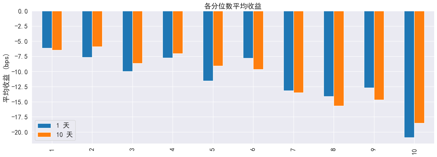
```python
# 生成统计图表
far.create_full_tear_sheet(
demeaned=False, group_adjust=False, by_group=False,
turnover_periods=None, avgretplot=(5, 15), std_bar=False
)
```
分位数统计
<div>
<style scoped>
.dataframe tbody tr th:only-of-type {
vertical-align: middle;
}
.dataframe tbody tr th {
vertical-align: top;
}
.dataframe thead th {
text-align: right;
}
</style>
<table border="1" class="dataframe">
<thead>
<tr style="text-align: right;">
<th></th>
<th>min</th>
<th>max</th>
<th>mean</th>
<th>std</th>
<th>count</th>
<th>count %</th>
</tr>
<tr>
<th>factor_quantile</th>
<th></th>
<th></th>
<th></th>
<th></th>
<th></th>
<th></th>
</tr>
</thead>
<tbody>
<tr>
<th>1</th>
<td>0.00000</td>
<td>0.30046</td>
<td>0.072019</td>
<td>0.056611</td>
<td>7293</td>
<td>10.054595</td>
</tr>
<tr>
<th>2</th>
<td>0.08846</td>
<td>0.49034</td>
<td>0.198844</td>
<td>0.066169</td>
<td>7266</td>
<td>10.017371</td>
</tr>
<tr>
<th>3</th>
<td>0.14954</td>
<td>0.65984</td>
<td>0.309961</td>
<td>0.089310</td>
<td>7219</td>
<td>9.952574</td>
</tr>
<tr>
<th>4</th>
<td>0.22594</td>
<td>0.80136</td>
<td>0.423978</td>
<td>0.111141</td>
<td>7248</td>
<td>9.992555</td>
</tr>
<tr>
<th>5</th>
<td>0.30904</td>
<td>0.99400</td>
<td>0.553684</td>
<td>0.133578</td>
<td>7280</td>
<td>10.036672</td>
</tr>
<tr>
<th>6</th>
<td>0.38860</td>
<td>1.23760</td>
<td>0.696531</td>
<td>0.166341</td>
<td>7211</td>
<td>9.941545</td>
</tr>
<tr>
<th>7</th>
<td>0.48394</td>
<td>1.56502</td>
<td>0.874488</td>
<td>0.204828</td>
<td>7240</td>
<td>9.981526</td>
</tr>
<tr>
<th>8</th>
<td>0.61900</td>
<td>2.09560</td>
<td>1.132261</td>
<td>0.265739</td>
<td>7226</td>
<td>9.962225</td>
</tr>
<tr>
<th>9</th>
<td>0.84984</td>
<td>3.30790</td>
<td>1.639863</td>
<td>0.436992</td>
<td>7261</td>
<td>10.010478</td>
</tr>
<tr>
<th>10</th>
<td>1.23172</td>
<td>40.47726</td>
<td>4.276270</td>
<td>3.640945</td>
<td>7290</td>
<td>10.050459</td>
</tr>
</tbody>
</table>
</div>
-------------------------
收益分析
<div>
<style scoped>
.dataframe tbody tr th:only-of-type {
vertical-align: middle;
}
.dataframe tbody tr th {
vertical-align: top;
}
.dataframe thead th {
text-align: right;
}
</style>
<table border="1" class="dataframe">
<thead>
<tr style="text-align: right;">
<th></th>
<th>period_1</th>
<th>period_10</th>
</tr>
</thead>
<tbody>
<tr>
<th>Ann. alpha</th>
<td>-0.087</td>
<td>-0.060</td>
</tr>
<tr>
<th>beta</th>
<td>1.218</td>
<td>1.238</td>
</tr>
<tr>
<th>Mean Period Wise Return Top Quantile (bps)</th>
<td>-20.913</td>
<td>-18.530</td>
</tr>
<tr>
<th>Mean Period Wise Return Bottom Quantile (bps)</th>
<td>-6.156</td>
<td>-6.452</td>
</tr>
<tr>
<th>Mean Period Wise Spread (bps)</th>
<td>-14.757</td>
<td>-13.177</td>
</tr>
</tbody>
</table>
</div>
<Figure size 640x480 with 0 Axes>
<Figure size 640x480 with 0 Axes>
......(图片过多,此处内容演示已省略,请参考api说明使用)
-------------------------
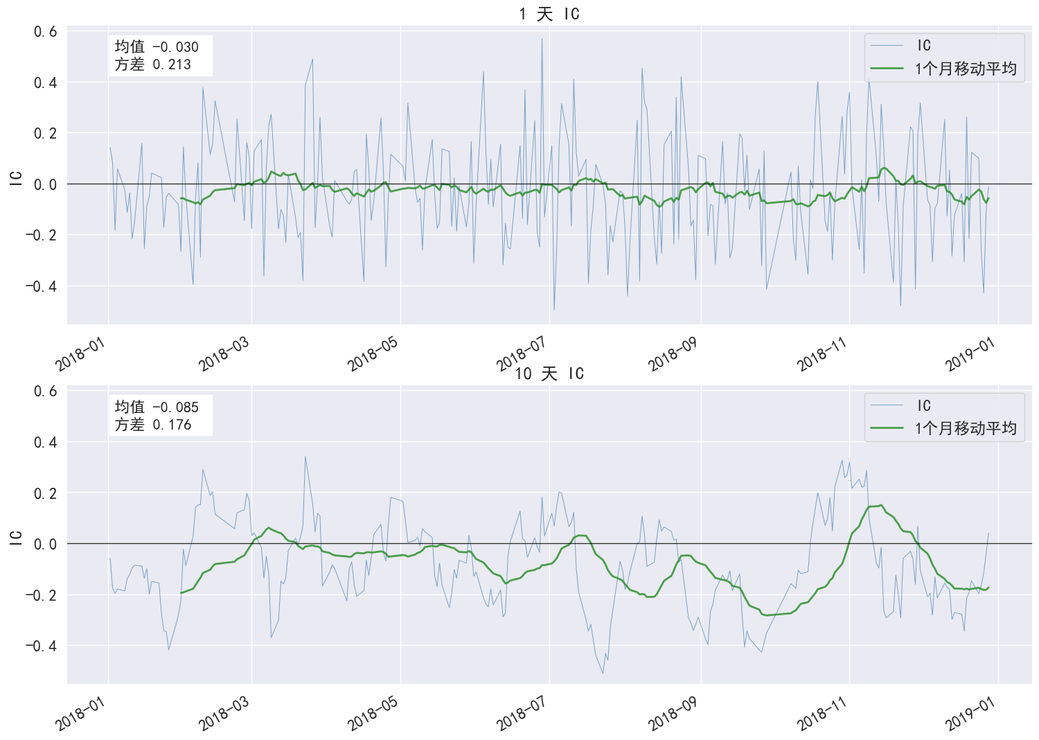
IC 分析
<div>
<style scoped>
.dataframe tbody tr th:only-of-type {
vertical-align: middle;
}
.dataframe tbody tr th {
vertical-align: top;
}
.dataframe thead th {
text-align: right;
}
</style>
<table border="1" class="dataframe">
<thead>
<tr style="text-align: right;">
<th></th>
<th>period_1</th>
<th>period_10</th>
</tr>
</thead>
<tbody>
<tr>
<th>IC Mean</th>
<td>-0.030</td>
<td>-0.085</td>
</tr>
<tr>
<th>IC Std.</th>
<td>0.213</td>
<td>0.176</td>
</tr>
<tr>
<th>IR</th>
<td>-0.140</td>
<td>-0.487</td>
</tr>
<tr>
<th>t-stat(IC)</th>
<td>-2.180</td>
<td>-7.587</td>
</tr>
<tr>
<th>p-value(IC)</th>
<td>0.030</td>
<td>0.000</td>
</tr>
<tr>
<th>IC Skew</th>
<td>0.240</td>
<td>0.091</td>
</tr>
<tr>
<th>IC Kurtosis</th>
<td>-0.420</td>
<td>-0.485</td>
</tr>
</tbody>
</table>
</div>
<Figure size 640x480 with 0 Axes>
<Figure size 640x480 with 0 Axes>
-------------------------
换手率分析
<div>
<style scoped>
.dataframe tbody tr th:only-of-type {
vertical-align: middle;
}
.dataframe tbody tr th {
vertical-align: top;
}
.dataframe thead th {
text-align: right;
}
</style>
<table border="1" class="dataframe">
<thead>
<tr style="text-align: right;">
<th></th>
<th>period_1</th>
<th>period_10</th>
</tr>
</thead>
<tbody>
<tr>
<th>Quantile 1 Mean Turnover</th>
<td>0.055</td>
<td>0.222</td>
</tr>
<tr>
<th>Quantile 2 Mean Turnover</th>
<td>0.136</td>
<td>0.447</td>
</tr>
<tr>
<th>Quantile 3 Mean Turnover</th>
<td>0.206</td>
<td>0.599</td>
</tr>
<tr>
<th>Quantile 4 Mean Turnover</th>
<td>0.268</td>
<td>0.680</td>
</tr>
<tr>
<th>Quantile 5 Mean Turnover</th>
<td>0.307</td>
<td>0.730</td>
</tr>
<tr>
<th>Quantile 6 Mean Turnover</th>
<td>0.337</td>
<td>0.742</td>
</tr>
<tr>
<th>Quantile 7 Mean Turnover</th>
<td>0.326</td>
<td>0.735</td>
</tr>
<tr>
<th>Quantile 8 Mean Turnover</th>
<td>0.279</td>
<td>0.708</td>
</tr>
<tr>
<th>Quantile 9 Mean Turnover</th>
<td>0.196</td>
<td>0.593</td>
</tr>
<tr>
<th>Quantile 10 Mean Turnover</th>
<td>0.073</td>
<td>0.283</td>
</tr>
</tbody>
</table>
</div>
<div>
<style scoped>
.dataframe tbody tr th:only-of-type {
vertical-align: middle;
}
.dataframe tbody tr th {
vertical-align: top;
}
.dataframe thead th {
text-align: right;
}
</style>
<table border="1" class="dataframe">
<thead>
<tr style="text-align: right;">
<th></th>
<th>period_1</th>
<th>period_10</th>
</tr>
</thead>
<tbody>
<tr>
<th>Mean Factor Rank Autocorrelation</th>
<td>0.991</td>
<td>0.884</td>
</tr>
</tbody>
</table>
</div>
......(图片过多,此处内容演示已省略,请参考api说明使用)
### 获取聚宽因子库数据的方法
[聚宽因子库](https://www.joinquant.com/help/api/help#name:factor_values)包含数百个质量、情绪、风险等其他类目的因子
连接jqdatasdk获取数据包,数据接口需调用聚宽 [jqdatasdk](https://www.joinquant.com/help/api/doc?name=JQDatadoc) 接口获取金融数据 ([试用注册地址](https://www.joinquant.com/default/index/sdk))
```python
# 获取因子数据:以5日平均换手率为例,该数据可以直接用于因子分析
# 具体使用方法可以参照jqdatasdk的API文档
import jqdatasdk
jqdatasdk.auth('username', 'password')
# 获取聚宽因子库中的VOL5数据
factor_data=jqdatasdk.get_factor_values(
securities=jqdatasdk.get_index_stocks('000300.XSHG'),
factors=['VOL5'],
start_date='2018-01-01',
end_date='2018-12-31')['VOL5']
```
### 将自有因子值转换成 DataFrame 格式的数据
- index 为日期,格式为 pandas 日期通用的 DatetimeIndex
- columns 为股票代码,格式要求符合聚宽的代码定义规则(如:平安银行的股票代码为 000001.XSHE)
- 如果是深交所上市的股票,在股票代码后面需要加入 .XSHE
- 如果是上交所上市的股票,在股票代码后面需要加入 .XSHG
- 将 pandas.DataFrame 转换成满足格式要求数据格式
首先要保证 index 为 DatetimeIndex 格式,一般是通过 pandas 提供的 pandas.to_datetime 函数进行转换,在转换前应确保 index 中的值都为合理的日期格式, 如 '2018-01-01' / '20180101',之后再调用 pandas.to_datetime 进行转换;另外应确保 index 的日期是按照从小到大的顺序排列的,可以通过 sort_index 进行排序;最后请检查 columns 中的股票代码是否都满足聚宽的代码定义。
```python
import pandas as pd
sample_data = pd.DataFrame(
[[0.84, 0.43, 2.33, 0.86, 0.96],
[1.06, 0.51, 2.60, 0.90, 1.09],
[1.12, 0.54, 2.68, 0.94, 1.12],
[1.07, 0.64, 2.65, 1.33, 1.15],
[1.21, 0.73, 2.97, 1.65, 1.19]],
index=['2018-01-02', '2018-01-03', '2018-01-04', '2018-01-05', '2018-01-08'],
columns=['000001.XSHE', '000002.XSHE', '000063.XSHE', '000069.XSHE', '000100.XSHE']
)
print(sample_data)
factor_data = sample_data.copy()
# 将 index 转换为 DatetimeIndex
factor_data.index = pd.to_datetime(factor_data.index)
# 将 DataFrame 按照日期顺序排列
factor_data = factor_data.sort_index()
# 检查 columns 是否满足聚宽股票代码格式
if not sample_data.columns.astype(str).str.match('\d{6}\.XSH[EG]').all():
print("有不满足聚宽股票代码格式的股票")
print(sample_data.columns[~sample_data.columns.astype(str).str.match('\d{6}\.XSH[EG]')])
print(factor_data)
```
- 将键为日期,值为各股票因子值的 Series 的 dict 转换成 pandas.DataFrame,可以直接利用 pandas.DataFrame 生成
```python
sample_data = \
{'2018-01-02': pd.Seris([0.84, 0.43, 2.33, 0.86, 0.96],
index=['000001.XSHE', '000002.XSHE', '000063.XSHE', '000069.XSHE', '000100.XSHE']),
'2018-01-03': pd.Seris([1.06, 0.51, 2.60, 0.90, 1.09],
index=['000001.XSHE', '000002.XSHE', '000063.XSHE', '000069.XSHE', '000100.XSHE']),
'2018-01-04': pd.Seris([1.12, 0.54, 2.68, 0.94, 1.12],
index=['000001.XSHE', '000002.XSHE', '000063.XSHE', '000069.XSHE', '000100.XSHE']),
'2018-01-05': pd.Seris([1.07, 0.64, 2.65, 1.33, 1.15],
index=['000001.XSHE', '000002.XSHE', '000063.XSHE', '000069.XSHE', '000100.XSHE']),
'2018-01-08': pd.Seris([1.21, 0.73, 2.97, 1.65, 1.19],
index=['000001.XSHE', '000002.XSHE', '000063.XSHE', '000069.XSHE', '000100.XSHE'])}
import pandas as pd
# 直接调用 pd.DataFrame 将 dict 转换为 DataFrame
factor_data = pd.DataFrame(data).T
print(factor_data)
# 之后请按照 DataFrae 的方法转换成满足格式要求数据格式
```
================================================
FILE: docs/API文档.md
================================================
# **API文档**
## 一、因子缓存factor_cache模块
为了在本地进行分析时,为了提高数据获取的速度并避免反复从服务端获取数据,所以增加了本地数据缓存的方法。
注意缓存格式为pyarrow.feather格式,pyarrow库不同版本之间可能存在兼容问题,建议不要随意修改pyarrow库的版本,如果修改后产生大量缓存文件无法读取(提示已损坏)的情况,建议删除整个缓存目录后重新缓存。
### 1. 设置缓存目录
对于单因子分析和归因分析中使用到的市值/价格和风格因子等数据,默认会缓存到用户的主目录( `os.path.expanduser( '~/jqfactor_datacache/bundle')` )。 一般地,在 Unix 系统上可能是 `/home/username/jqfactor_datacache/bundle`,而在 Windows 系统上可能是 `C:\Users\username\jqfactor_datacache\bundle`。
您可以通过以下代码修改配置信息来设置为其他路径,设置过一次后后续都将沿用设置的这个路径,不用重复设置。
```python
from jqfactor_analyzer.factor_cache import set_cache_dir,get_cache_dir
set_cache_dir(my_path) #设置缓存目录为my_path
print(get_cache_dir()) #输出缓存目录
```
### 2. 缓存/检查缓存和读取已缓存数据
除过对单因子分析及归因分析依赖的数据进行缓存外,factor_cache还可以缓存自定义的因子组(仅限聚宽因子库中支持的因子)
```python
def save_factor_values_by_group(start_date,end_date,factor_names='prices',
group_name=None,overwrite=False,cache_dir=None,show_progress=True):
"""将因子库数据按因子组储存到本地,根据factor_names因子列表(顺序无关)自动生成因子组的名称
start_date : 开始时间
end_date : 结束时间
factor_names : 因子组所含因子的名称,除过因子库中支持的因子外,还支持指定为'prices'缓存价格数据
group_name : 因子组名称,不指定时使用get_factor_folder自动生成因子组名(即缓存文件夹名),如果指定则按照指定的名称生成文件夹名(使用get_factor_values_by_cache时,需要自行指定factor_path)
overwrite : 文件已存在时是否覆盖更新,默认为False即增量更新,文件已存在时跳过
cache_dir : 缓存的路径,如果没有指定则使用配置信息中的路径,一般不用指定
show_progress : 是否展示缓存进度,默认为True
返回 : 因子组储存的路径 , 文件以天为单位储存为feather文件,每天一个feather文件,每月一个文件夹,columns为因子名称, index为当天在市的所有标的代码
"""
def get_factor_values_by_cache(date,codes=None,factor_names=None,group_name=None,
factor_path=None):
"""从缓存的文件读取因子数据,文件不存在时返回空的dataframe
date : 日期
codes : 标的代码,默认为None获取当天在市的所有标的
factor_names : 因子列表(顺序无关),当指定factor_path/group_name时失效
group_name : 因子组名,如果缓存时指定了group_name,则获取时必须也指定group_name或factor_path
factor_path : 可选参数,因子组的路径,一般不用指定
返回:
如果缓存文件存在,则返回当天的因子数据,index是标的代码,columns是因子名
如果缓存文件不存在,则返回空的dataframe, 建议在使用get_factor_values_by_cache前,先运行save_factor_values_by_group检查时间区间内的缓存文件是否完整
"""
def get_factor_folder(factor_names,group_name=None):
"""获取因子组的文件夹名(文件夹位于get_cache_dir()获取的缓存目录下)
factor_names : 因子储存时,如果未指定group_name,则根据因子列表(顺序无关)获取md5值生成因子组名(即储存的文件夹名),使用此方法可以获取生成的文件夹名称
group_name : 如果储存时指定了因子组名,则直接返回此因子组名
"""
```
**示例**
```python
from jqfactor_analyzer.factor_cache import save_factor_values_by_group,get_factor_values_by_cache,get_factor_folder,get_cache_dir
# import jqdatasdk as jq
# jq.auth("账号",'密码') #登陆jqdatasdk来从服务端缓存数据
all_factors = jq.get_all_factors()
factor_names = all_factors[all_factors.category=='growth'].factor.tolist() #将聚宽因子库中的成长类因子作为一组因子
group_name = 'growth_factors' #因子组名定义为'growth_factors'
start_date = '2021-01-01'
end_date = '2021-06-01'
# 检查/缓存因子数据
factor_path = save_factor_values_by_group(start_date,end_date,factor_names=factor_names,group_name=group_name,overwrite=False,show_progress=True)
# factor_path = os.path.join(get_cache_dir(), get_factor_folder(factor_names,group_name=group_name) #等同于save_factor_values_by_group返回的路径
# 循环获取缓存的因子数据,并拼接
trade_days = jq.get_trade_days(start_date,end_date)
factor_values = {}
for date in trade_days:
factor_values[date] = get_factor_values_by_cache(date,codes=None,factor_names=factor_names,group_name=group_name, factor_path=factor_path)#这里实际只需要指定group_name,factor_names参数的其中一个,缓存时指定了group_name时,factor_names不生效
factor_values = pd.concat(factor_values)
```
## 二、归因分析模块
```python
from jqfactor_analyzer import AttributionAnalysis
AttributionAnalysis(weights,daily_return,style_type='style_pro',industry ='sw_l1',use_cn=True,show_data_progress=True)
```
**参数 :**
- `weights`:持仓权重信息,index是日期,columns是标的代码, value对应的是组合当天的仓位占比(单日仓位占比总和不为1时,剩余部分认为是当天的现金)
- `daily_return`:Series,index是日期,values为当天组合的收益率
- `style_type`:归因分析所使用的风格因子类型,可选'style'和'style_pro'中的一个
- `industry`:归因分析所使用的行业分类,可选'sw_l1'和'jq_l1'中的一个
- `use_cn`:绘图时是否使用中文
- `show_data_progress`:是否展示数据获取进度(使用本地缓存,第一次运行时速度较慢,后续对于本地不存在的数据将增量缓存)
**示例**
```python
import pandas as pd
# position_weights.csv 是一个储存了组合权重信息的csv文件,index是日期,columns是股票代码
# position_daily_return.csv 是一个储存了组合日收益率的csv文件,index是日期,daily_return列是日收益
weights = pd.read_csv("position_weights.csv",index_col=0)
returns = pd.read_csv("position_daily_return.csv",index_col=0)['daily_return']
An = AttributionAnalysis(weights , returns ,style_type='style_pro',industry ='sw_l1', show_data_progress=True )
```
### 1. 属性
- `style_exposure` : 组合的风格暴露
- `industry_exposure` : 组合的行业暴露
- `exposure_portfolio` : 组合的风格+行业及country暴露
- `attr_daily_returns` : 组合的\风格+行业及country日度归因收益率
- `attr_returns` : 组合的日度风格+行业及country累积归因收益率
### 2. 方法
#### (1) 获取组合相对于指数的暴露
```python
get_exposure2bench(index_symbol)
```
**参数 :**
- `index_symbol` : 基准指数, 可选`['000300.XSHG','000905.XSHG','000906.XSHG','000852.XSHG','932000.CSI','000985.XSHG']`中的一个
**返回 :**
- 一个dataframe,index为日期,columns为风格因子+行业因子+county , 其中country为股票总持仓占比
#### (2) 获取组合相对于指数的日度归因收益率
```python
get_attr_daily_returns2bench(index_symbol)
```
假设组合相对于指数的收益由以下部分构成 : 风格+行业暴露收益(common_return ) , 现金闲置收益(cash) ,策略本身的超额收益(specific_return)
**参数 :**
- `index_symbol` : 基准指数, 可选`['000300.XSHG','000905.XSHG','000906.XSHG','000852.XSHG','932000.CSI','000985.XSHG']`中的一个
**返回 :**
- 一个dataframe,index为日期,columns为`风格因子+行业因子+cash+common_return,specific_return,total_return`
其中:
cash是假设现金收益(0)相对指数带来的收益率
common_return 为风格+行业总收益率
specific_return 为特意收益率
total_return 为组合相对于指数的总收益
#### (3) 获取相对于指数的累积归因收益率
```python
get_attr_returns2bench(index_symbol)
```
假设组合相对于指数的收益由以下部分构成 : 风格+行业暴露收益(common_return ) , 现金闲置收益(cash) ,策略本身的超额收益(specific_return)
**参数 :**
`index_symbol` : 基准指数, 可选`['000300.XSHG','000905.XSHG','000906.XSHG','000852.XSHG','932000.CSI','000985.XSHG']`中的一个
**返回 :**
- 一个dataframe,index为日期,columns为`风格因子+行业因子+cash+common_return,specific_return,total_return`
其中:
cash是假设现金收益(0)相对指数带来的收益率
common_return 为风格+行业总收益率
specific_return 为特异收益率
total_return 为组合相对于指数的总收益(减法超额)
### 3. 绘图方法
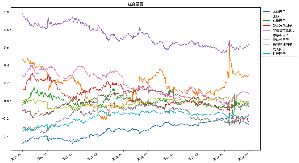
#### (1) 绘制风格暴露时序图
```python
plot_exposure(factors='style',index_symbol=None,figsize=(15,7))
```
绘制风格暴露时序
**参数**
- factors : 绘制的暴露类型 , 可选 'style'(所有风格因子) , 'industry'(所有行业因子),也可以传递一个list,list为exposure_portfolio中columns的一个或者多个
- index_symbol : 基准指数代码,指定时绘制相对于指数的暴露 , 默认None为组合本身的暴露
- figsize : 画布大小
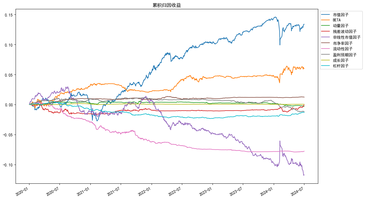
#### (2) 绘制归因分析收益时序图
```python
plot_returns(factors='style',index_symbol=None,figsize=(15,7))
```
绘制归因分析收益时序
**参数**
- factors : 绘制的暴露类型 , 可选 'style'(所有风格因子) , 'industry'(所有行业因子),也可以传递一个list,list为exposure_portfolio中columns的一个或者多个
同时也支持指定['common_return'(风格总收益),'specific_return'(特异收益),'total_return'(总收益)', 'country'(国家因子收益,当指定index_symbol时会用现金相对于指数的收益替代)]
- index_symbol : 基准指数代码,指定时绘制相对于指数的暴露 , 默认None为组合本身的暴露
- figsize : 画布大小
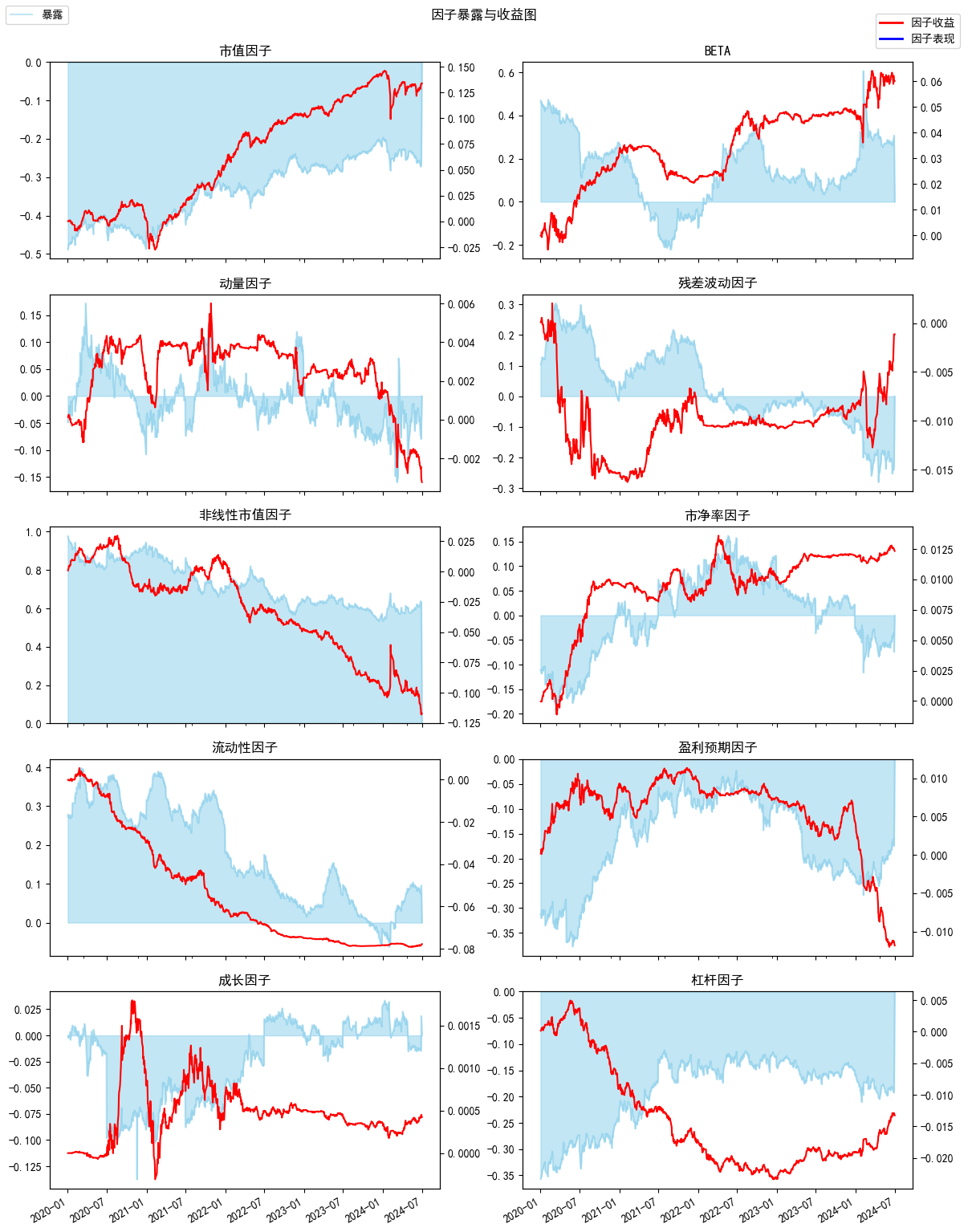
#### (3) 绘制暴露与收益对照图
```python
plot_exposure_and_returns(factors='style',index_symbol=None,show_factor_perf=False,figsize=(12,6))
```
将因子暴露与收益同时绘制在多个子图上
**参数**
- factors : 绘制的暴露类型 , 可选 'style'(所有风格因子) , 'industry'(所有行业因子,也可以传递一个list,list为exposure_portfolio中columns的一个或者多个
当指定index_symbol时,country会用现金相对于指数的收益替代)
- index_symbol : 基准指数代码,指定时绘制相对于指数的暴露及收益 , 默认None为组合本身的暴露和收益
- show_factor_perf : 是否同时绘制因子表现
- figsize : 画布大小,这里第一个参数是画布的宽度, 第二个参数为单个子图的高度
#### (4) 关闭中文图例显示
```python
plot_disable_chinese_label()
```
画图时默认会从系统中查找中文字体显示以中文图例
如果找不到中文字体则默认使用英文图例
当找到中文字体但中文显示乱码时, 可调用此 API 关闭中文图例显示而使用英文
## 三、单因子分析模块
```python
from jqfactor_analyzer import analyze_factor
analyze_factor(factor, industry='jq_l1', quantiles=5, periods=(1, 5, 10), weight_method='avg', max_loss=0.25, allow_cache=True, show_data_progress=True )
```
单因子分析函数
**参数**
* `factor`: 因子值,
pandas.DataFrame格式的数据
- index为日期,格式为pandas日期通用的DatetimeIndex,转换方法见[将自有因子值转换成 DataFrame 格式的数据](#将自有因子值转换成-dataframe-格式的数据)
- columns为股票代码,格式要求符合聚宽的代码定义规则(如:平安银行的股票代码为000001.XSHE)
- 如果是深交所上市的股票,在股票代码后面需要加入.XSHE
- 如果是上交所上市的股票,在股票代码后面需要加入.XSHG
或 pd.Series格式的数据
- index为日期和股票代码组成的MultiIndex
* `industry`: 行业分类, 默认为 `'jq_l1'`
* `'sw_l1'`: 申万一级行业
* `'sw_l2'`: 申万二级行业
* `'sw_l3'`: 申万三级行业
* `'jq_l1'`: 聚宽一级行业
* `'jq_l2'`: 聚宽二级行业
* `'zjw'`: 证监会行业
* `quantiles`: 分位数数量, 默认为 `5`
`int`
在因子分组中按照因子值大小平均分组的组数.
* `periods`: 调仓周期, 默认为 [1, 5, 10]
`int` or `list[int]`
* `weight_method`: 基于分位数收益时的加权方法, 默认为 `'avg'`
* `'avg'`: 等权重
* `'mktcap'`:按总市值加权
* `'ln_mktcap'`: 按总市值的对数加权
* `'cmktcap'`: 按流通市值加权
* `'ln_cmktcap'`: 按流通市值的对数加权
* `max_loss`: 因重复值或nan值太多而无效的因子值的最大占比, 默认为 0.25
`float`
允许的丢弃因子数据的最大百分比 (0.00 到 1.00),
计算比较输入因子索引中的项目数和输出 DataFrame 索引中的项目数.
因子数据本身存在缺陷 (例如 NaN),
没有提供足够的价格数据来计算所有因子值的远期收益,
或者因为分组失败, 因此可以部分地丢弃因子数据
* `allow_cache` : 是否允许对价格,市值等信息进行本地缓存(按天缓存,初次运行可能比较慢,但后续重新获取对应区间的数据将非常快,且分析时仅消耗较小的jqdatasdk流量)
* show_data_progress: 是否展示数据获取的进度信息
**示例**
```python
#载入函数库
import pandas as pd
import jqfactor_analyzer as ja
# 获取 jqdatasdk 授权
# 输入用户名、密码,申请地址:http://t.cn/EINDOxE
# 聚宽官网及金融终端,使用方法参见:http://t.cn/EINcS4j
import jqdatasdk
jqdatasdk.auth('username', 'password')
# 对因子进行分析
far = ja.analyze_factor(
factor_data, # factor_data 为因子值的 pandas.DataFrame
quantiles=10,
periods=(1, 10),
industry='jq_l1',
weight_method='avg',
max_loss=0.1
)
# 生成统计图表
far.create_full_tear_sheet(
demeaned=False, group_adjust=False, by_group=False,
turnover_periods=None, avgretplot=(5, 15), std_bar=False
)
```
### 1. 绘制结果
#### 展示全部分析
```
far.create_full_tear_sheet(demeaned=False, group_adjust=False, by_group=False,
turnover_periods=None, avgretplot=(5, 15), std_bar=False)
```
**参数:**
- demeaned:
- True: 使用超额收益计算 (基准收益被认为是每日所有股票收益按照weight列中权重加权的均值)
- False: 不使用超额收益
- group_adjust:
- True: 使用行业中性化后的收益计算 (行业收益被认为是每日各个行业股票收益按照weight列中权重加权的均值)
- False: 不使用行业中性化后的收益
- by_group:
- True: 按行业展示
- False: 不按行业展示
- turnover_periods: 调仓周期
- avgretplot: tuple 因子预测的天数-(计算过去的天数, 计算未来的天数)
- std_bar:
- True: 显示标准差
- False: 不显示标准差
#### 因子值特征分析
```
far.create_summary_tear_sheet(demeaned=False, group_adjust=False)
```
**参数:**
- demeaned:
- True: 对每日因子收益去均值求得因子收益表
- False: 因子收益表
- group_adjust:
- True: 按行业对因子收益去均值后求得因子收益表
- False: 因子收益表
#### 因子收益分析
```
far.create_returns_tear_sheet(demeaned=False, group_adjust=False, by_group=False)
```
**参数:**
- demeaned:
- True: 使用超额收益计算 (基准收益被认为是每日所有股票收益按照weight列中权重加权的均值)
- False: 不使用超额收益
- group_adjust:
- True: 使用行业中性化后的收益计算 (行业收益被认为是每日各个行业股票收益按照weight列中权重加权的均值)
- False: 不使用行业中性化后的收益
- by_group:
- True: 画各行业的各分位数平均收益图
- False: 不画各行业的各分位数平均收益图
#### 因子 IC 分析
```
far.create_information_tear_sheet(group_adjust=False, by_group=False)
```
**参数:**
- group_adjust:
- True: 使用行业中性收益 (行业收益被认为是每日各个行业股票收益按照weight列中权重的加权的均值)
- False: 不使用行业中性收益
- by_group:
- True: 画按行业分组信息比率(IC)图
- False: 画月度信息比率(IC)图
#### 因子换手率分析
```
far.create_turnover_tear_sheet(turnover_periods=None)
```
**参数:**
- turnover_periods: 调仓周期
#### 因子预测能力分析
```
far.create_event_returns_tear_sheet(avgretplot=(5, 15),demeaned=False, group_adjust=False,std_bar=False)
```
**参数:**
- avgretplot: tuple 因子预测的天数-(计算过去的天数, 计算未来的天数)
- demeaned:
- True: 使用超额收益计算累积收益 (基准收益被认为是每日所有股票收益按照weight列中权重加权的均值)
- False: 不使用超额收益
- group_adjust:
- True: 使用行业中性化后的收益计算累积收益 (行业收益被认为是每日各个行业股票收益按照weight列中权重加权的均值)
- False: 不使用行业中性化后的收益
- std_bar:
- True: 显示标准差
- False: 不显示标准差
#### 打印因子收益表
```
far.plot_returns_table(demeaned=False, group_adjust=False)
```
**参数:**
- demeaned:
- True:使用超额收益计算 (基准收益被认为是每日所有股票收益按照weight列中权重的加权的均值)
- False:不使用超额收益
- group_adjust:
- True:使用行业中性收益 (行业收益被认为是每日各个行业股票收益按照weight列中权重的加权的均值)
- False:不使用行业中性收益
#### 打印换手率表
```
far.plot_turnover_table()
```
#### 打印信息比率(IC)相关表
```
far.plot_information_table(group_adjust=False, method='rank')
```
**参数:**
- group_adjust:
- True:使用行业中性收益 (行业收益被认为是每日各个行业股票收益按照weight列中权重的加权的均值)
- False:不使用行业中性收益
- method:
- 'rank':用秩相关系数计算IC值
- 'normal': 用相关系数计算IC值
#### 打印个分位数统计表
```
far.plot_quantile_statistics_table()
```
#### 画信息比率(IC)时间序列图
```
far.plot_ic_ts(group_adjust=False, method='rank')
```
**参数:**
- group_adjust:
- True:使用行业中性收益 (行业收益被认为是每日各个行业股票收益按照weight列中权重的加权的均值)
- False:不使用行业中性收益
- method:
- 'rank':用秩相关系数计算IC值
- 'normal': 用相关系数计算IC值
#### 画信息比率分布直方图
```
far.plot_ic_hist(group_adjust=False, method='rank')
```
**参数:**
- group_adjust:
- True:使用行业中性收益 (行业收益被认为是每日各个行业股票收益按照weight列中权重的加权的均值)
- False:不使用行业中性收益
- method:
- 'rank':用秩相关系数计算IC值
- 'normal': 用相关系数计算IC值
#### 画信息比率 qq 图
```
far.plot_ic_qq(group_adjust=False, method='rank', theoretical_dist='norm')
```
**参数:**
- group_adjust:
- True:使用行业中性收益 (行业收益被认为是每日各个行业股票收益按照weight列中权重的加权的均值)
- False:不使用行业中性收益
- method:
- 'rank':用秩相关系数计算IC值
- 'normal': 用相关系数计算IC值
- theoretical_dist:
- 'norm':正态分布
- 't':t分布
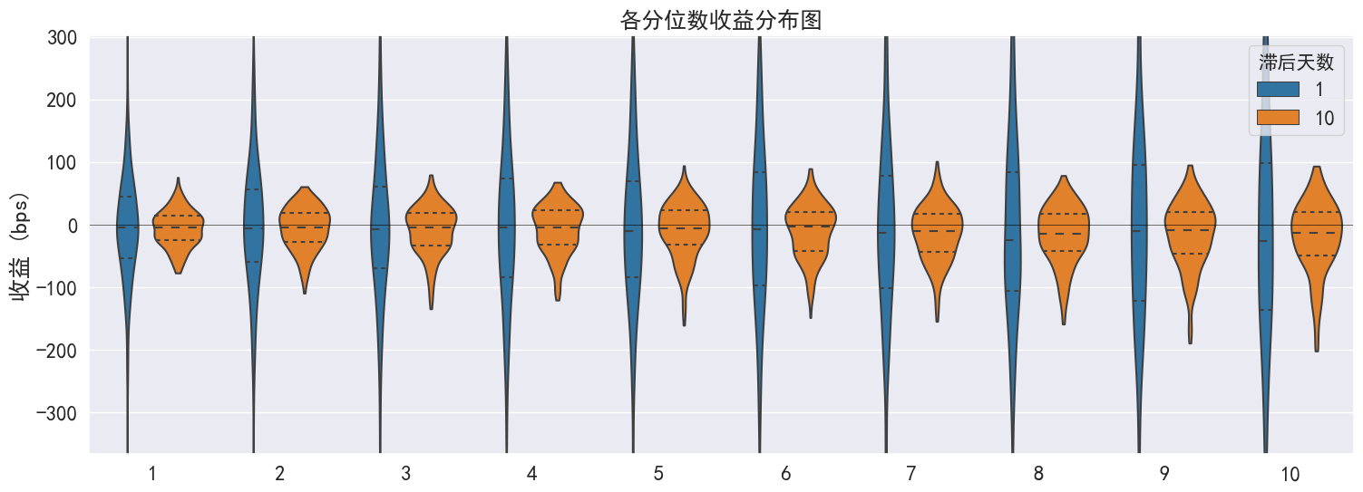
#### 画各分位数平均收益图
```
far.plot_quantile_returns_bar(by_group=False, demeaned=False, group_adjust=False)
```
**参数:**
- by_group:
- True:各行业的各分位数平均收益图
- False:各分位数平均收益图
- demeaned:
- True:使用超额收益计算累积收益 (基准收益被认为是每日所有股票收益按照weight列中权重加权的均值)
- False:不使用超额收益
- group_adjust:
- True:使用行业中性化后的收益计算累积收益 (行业收益被认为是每日各个行业股票收益按照weight列中权重加权的均值)
- False:不使用行业中性化后的收益
#### 画最高分位减最低分位收益图
```
far.plot_mean_quantile_returns_spread_time_series(demeaned=False, group_adjust=False, bandwidth=1)
```
**参数:**
- demeaned:
- True:使用超额收益计算累积收益 (基准收益被认为是每日所有股票收益按照weight列中权重加权的均值)
- False:不使用超额收益
- group_adjust:
- True:使用行业中性化后的收益计算累积收益 (行业收益被认为是每日各个行业股票收益按照weight列中权重加权的均值)
- False:不使用行业中性化后的收益
- bandwidth:n,加减n倍当日标准差
#### 画按行业分组信息比率(IC)图
```
far.plot_ic_by_group(group_adjust=False, method='rank')
```
**参数:**
- group_adjust:
- True:使用行业中性收益 (行业收益被认为是每日各个行业股票收益按照weight列中权重的加权的均值)
- False:不使用行业中性收益
- method:
- 'rank':用秩相关系数计算IC值
- 'normal': 用相关系数计算IC值
#### 画因子自相关图
```
far.plot_factor_auto_correlation(rank=True)
```
**参数:**
- rank:
- True:用秩相关系数
- False:用相关系数
#### 画最高最低分位换手率图
```
far.plot_top_bottom_quantile_turnover(periods=(1, 3, 9))
```
**参数:**
- periods:调仓周期
#### 画月度信息比率(IC)图
```
far.plot_monthly_ic_heatmap(group_adjust=False)
```
**参数:**
- group_adjust:
- True:使用行业中性收益 (行业收益被认为是每日各个行业股票收益按照weight列中权重的加权的均值)
- False:不使用行业中性收益
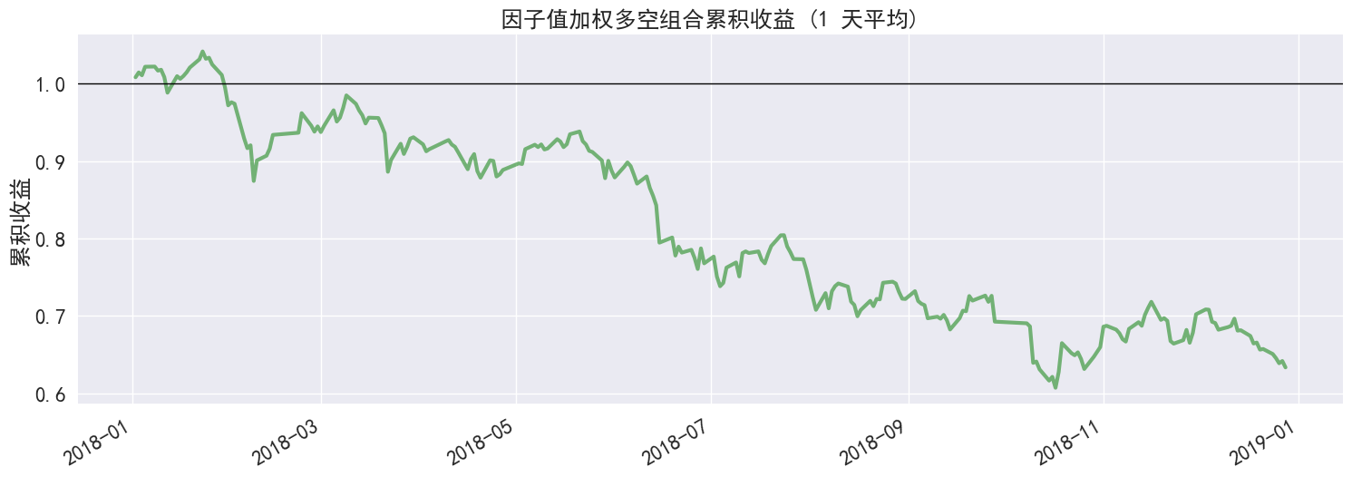
#### 画按因子值加权多空组合每日累积收益图
```
far.plot_cumulative_returns(period=1, demeaned=False, group_adjust=False)
```
**参数:**
- periods:调仓周期
- demeaned:
- True:对因子值加权组合每日收益的权重去均值 (每日权重 = 每日权重 - 每日权重的均值),使组合转换为cash-neutral多空组合
- False:不对权重去均值
- group_adjust:
- True:对权重分行业去均值 (每日权重 = 每日权重 - 每日各行业权重的均值),使组合转换为 industry-neutral 多空组合
- False:不对权重分行业去均值
#### 画做多最大分位数做空最小分位数组合每日累积收益图
```
far.plot_top_down_cumulative_returns(period=1, demeaned=False, group_adjust=False)
```
**参数:**
- periods:指定调仓周期
- demeaned:
- True:使用超额收益计算累积收益 (基准收益被认为是每日所有股票收益按照weight列中权重加权的均值)
- False:不使用超额收益
- group_adjust:
- True:使用行业中性化后的收益计算累积收益 (行业收益被认为是每日各个行业股票收益按照weight列中权重加权的均值)
- False:不使用行业中性化后的收益
#### 画各分位数每日累积收益图
```
far.plot_cumulative_returns_by_quantile(period=(1, 3, 9), demeaned=False, group_adjust=False)
```
**参数:**
- periods:调仓周期
- demeaned:
- True:使用超额收益计算累积收益 (基准收益被认为是每日所有股票收益按照weight列中权重加权的均值)
- False:不使用超额收益
- group_adjust:
- True:使用行业中性化后的收益计算累积收益 (行业收益被认为是每日各个行业股票收益按照weight列中权重加权的均值)
- False:不使用行业中性化后的收益
#### 因子预测能力平均累计收益图
```
far.plot_quantile_average_cumulative_return(periods_before=5, periods_after=10, by_quantile=False, std_bar=False, demeaned=False, group_adjust=False)
```
**参数:**
- periods_before: 计算过去的天数
- periods_after: 计算未来的天数
- by_quantile:
- True:各分位数分别显示因子预测能力平均累计收益图
- False:不用各分位数分别显示因子预测能力平均累计收益图
- std_bar:
- True:显示标准差
- False:不显示标准差
- demeaned:
- True: 使用超额收益计算累积收益 (基准收益被认为是每日所有股票收益按照weight列中权重加权的均值)
- False: 不使用超额收益
- group_adjust:
- True: 使用行业中性化后的收益计算累积收益 (行业收益被认为是每日各个行业股票收益按照weight列中权重加权的均值)
- False: 不使用行业中性化后的收益
#### 画有效因子数量统计图
```
far.plot_events_distribution(num_days=1)
```
**参数:**
- num_days:统计间隔天数
#### 关闭中文图例显示
```
far.plot_disable_chinese_label()
```
### 2. 属性列表
用于访问因子分析的结果,大部分为惰性属性,在访问才会计算结果并返回
#### 查看因子值
```
far.factor_data
```
- 类型:pandas.Series
- index:为日期和股票代码的MultiIndex
#### 去除 nan/inf,整理后的因子值、forward_return 和分位数
```
far.clean_factor_data
```
- 类型:pandas.DataFrame index:为日期和股票代码的MultiIndex
- columns:根据period选择后的forward_return(如果调仓周期为1天,那么forward_return为[第二天的收盘价-今天的收盘价]/今天的收盘价)、因子值、行业分组、分位数数组、权重
#### 按分位数分组加权平均因子收益
```
far.mean_return_by_quantile
```
- 类型:pandas.DataFrame
- index:分位数分组
- columns:调仓周期
#### 按分位数分组加权因子收益标准差
```
far.mean_return_std_by_quantile
```
- 类型:pandas.DataFrame
- index:分位数分组
- columns:调仓周期
#### 按分位数及日期分组加权平均因子收益
```
far.mean_return_by_date
```
- 类型:pandas.DataFrame
- index:为日期和分位数的MultiIndex
- columns:调仓周期
#### 按分位数及日期分组加权因子收益标准差
```
far.mean_return_std_by_date
```
- 类型:pandas.DataFrame
- index:为日期和分位数的MultiIndex
- columns:调仓周期
#### 按分位数及行业分组加权平均因子收益
```
far.mean_return_by_group
```
- 类型:pandas.DataFrame
- index:为行业和分位数的MultiIndex
- columns:调仓周期
#### 按分位数及行业分组加权因子收益标准差
```
far.mean_return_std_by_group
```
- 类型:pandas.DataFrame
- index:为行业和分位数的MultiIndex
- columns:调仓周期
#### 最高分位数因子收益减最低分位数因子收益每日均值
```
far.mean_return_spread_by_quantile
```
- 类型:pandas.DataFrame
- index:日期
- columns:调仓周期
#### 最高分位数因子收益减最低分位数因子收益每日标准差
```
far.mean_return_spread_std_by_quantile
```
- 类型:pandas.DataFrame
- index:日期
- columns:调仓周期
#### 信息比率
```
far.ic
```
- 类型:pandas.DataFrame
- index:日期
- columns:调仓周期
#### 分行业信息比率
```
far.ic_by_group
```
- 类型:pandas.DataFrame
- index:行业
- columns:调仓周期
#### 月度信息比率
```
far.ic_monthly
```
- 类型:pandas.DataFrame
- index:月度
- columns:调仓周期表
#### 换手率
```
far.quantile_turnover
```
- 键:调仓周期
- 值: pandas.DataFrame 换手率
- index:日期
- columns:分位数分组
#### 计算按分位数分组加权因子收益和标准差
```
mean, std = far.calc_mean_return_by_quantile(by_date=True, by_group=False, demeaned=False, group_adjust=False)
```
**参数:**
- by_date:
- True:按天计算收益
- False:不按天计算收益
- by_group:
- True: 按行业计算收益
- False:不按行业计算收益
- demeaned:
- True:使用超额收益计算各分位数收益,超额收益=收益-基准收益 (基准收益被认为是每日所有股票收益按照weight列中权重的加权的均值)
- False:不使用超额收益
- group_adjust:
- True:使用行业中性收益计算各分位数收益,行业中性收益=收益-行业收益 (行业收益被认为是每日各个行业股票收益按照weight列中权重的加权的均值)
- False:不使用行业中性收益
#### 计算按因子值加权多空组合每日收益
```
far.calc_factor_returns(demeaned=True, group_adjust=False)
```
权重 = 每日因子值 / 每日因子值的绝对值的和
正的权重代表买入, 负的权重代表卖出
**参数:**
- demeaned:
- True: 对权重去均值 (每日权重 = 每日权重 - 每日权重的均值), 使组合转换为 cash-neutral 多空组合
- False:不对权重去均值
- group_adjust:
- True:对权重分行业去均值 (每日权重 = 每日权重 - 每日各行业权重的均值),使组合转换为 industry-neutral 多空组合
- False:不对权重分行业去均值
#### 计算两个分位数相减的因子收益和标准差
```
mean, std = far.compute_mean_returns_spread(upper_quant=None, lower_quant=None, by_date=False, by_group=False, demeaned=False, group_adjust=False)
```
**参数:**
- upper_quant:用upper_quant选择的分位数减去lower_quant选择的分位数,只能在已有的范围内选择
- lower_quant:用upper_quant选择的分位数减去lower_quant选择的分位数,只能在已有的范围内选择
- by_date:
- True:按天计算两个分位数相减的因子收益和标准差
- False:不按天计算两个分位数相减的因子收益和标准差
- by_group:
- True: 分行业计算两个分位数相减的因子收益和标准差
- False:不分行业计算两个分位数相减的因子收益和标准差
- demeaned:
- True:使用超额收益 (基准收益被认为是每日所有股票收益按照weight列中权重加权的均值)
- False:不使用超额收益
- group_adjust:
- True:使用行业中性收益 (行业收益被认为是每日各个行业股票收益按照weight列中权重加权的均值)
- False:不使用行业中性收益
#### 计算因子的 alpha 和 beta
```
far.calc_factor_alpha_beta(demeaned=True, group_adjust=False)
```
因子值加权组合每日收益 = beta * 市场组合每日收益 + alpha
因子值加权组合每日收益计算方法见 calc_factor_returns 函数
市场组合每日收益是每日所有股票收益按照weight列中权重加权的均值
结果中的 alpha 是年化 alpha
**参数:**
- demeaned:
- True: 对因子值加权组合每日收益的权重去均值 (每日权重 = 每日权重 - 每日权重的均值),使组合转换为cash-neutral多空组合
- False:不对权重去均值
- group_adjust:
- True:对权重分行业去均值 (每日权重 = 每日权重 - 每日各行业权重的均值),使组合转换为 industry-neutral 多空组合
- False:不对权重分行业去均值
#### 计算每日因子信息比率(IC值)
```
far.calc_factor_information_coefficient(group_adjust=False, by_group=False, method='rank')
```
**参数:**
- group_adjust:
- True:使用行业中性收益计算 IC (行业收益被认为是每日各个行业股票收益按照weight列中权重加权的均值)
- False:不使用行业中性收益
- by_group:
- True:分行业计算 IC
- False:不分行业计算 IC
- method:
- 'rank':用秩相关系数计算IC值
- 'normal':用普通相关系数计算IC值
#### 计算因子信息比率均值(IC值均值)
```
far.calc_mean_information_coefficient(group_adjust=False, by_group=False, by_time=None, method='rank')
```
**参数:**
- group_adjust:
- True:使用行业中性收益计算 IC (行业收益被认为是每日各个行业股票收益按照weight列中权重加权的均值)
- False:不使用行业中性收益
- by_group:
- True:分行业计算 IC
- False:不分行业计算 IC
- by_time:
- 'Y':按年求均值
- 'M':按月求均值
- None:对所有日期求均值
- method:
- 'rank':用秩相关系数计算IC值
- 'normal':用普通相关系数计算IC值
#### 按照当天的分位数算分位数未来和过去的收益均值和标准差
```
far.calc_average_cumulative_return_by_quantile(periods_before=5, periods_after=15, demeaned=False, group_adjust=False)
```
**参数:**
- periods_before:计算过去的天数
- periods_after:计算未来的天数
- demeaned:
- True:使用超额收益计算累积收益 (基准收益被认为是每日所有股票收益按照weight列中权重加权的均值)
- False:不使用超额收益
- group_adjust:
- True:使用行业中性化后的收益计算累积收益
- False:不使用行业中性化后的收益
#### 计算指定调仓周期的各分位数每日累积收益
```
far.calc_cumulative_return_by_quantile(period=None, demeaned=False, group_adjust=False)
```
**参数:**
- period:指定调仓周期
- demeaned:
- True:使用超额收益计算累积收益 (基准收益被认为是每日所有股票收益按照weight列中权重加权的均值)
- False:不使用超额收益
- group_adjust:
- True:使用行业中性化后的收益计算累积收益
- False:不使用行业中性化后的收益
#### 计算指定调仓周期的按因子值加权多空组合每日累积收益
```
far.calc_cumulative_returns(period=5, demeaned=False, group_adjust=False)
```
当 period > 1 时,组合的累积收益计算方法为:
组合每日收益 = (从第0天开始每period天一调仓的组合每日收益 + 从第1天开始每period天一调仓的组合每日收益 + ... + 从第period-1天开始每period天一调仓的组合每日收益) / period
组合累积收益 = 组合每日收益的累积
**参数:**
- period:指定调仓周期
- demeaned:
- True:对权重去均值 (每日权重 = 每日权重 - 每日权重的均值),使组合转换为 cash-neutral 多空组合
- False:不对权重去均值
- group_adjust:
- True:对权重分行业去均值 (每日权重 = 每日权重 - 每日各行业权重的均值),使组合转换为 industry-neutral 多空组合
- False:不对权重分行业去均值
#### 计算指定调仓周期和前面定义好的加权方式计算多空组合每日累计收益
```
far.calc_top_down_cumulative_returns(period=5, demeaned=False, group_adjust=False)
```
**参数:**
- period:指定调仓周期
- demeaned:
- True:使用超额收益计算累积收益 (基准收益被认为是每日所有股票收益按照weight列中权重加权的均值)
- False:不使用超额收益
- group_adjust:
- True:使用行业中性化后的收益计算累积收益 (行业收益被认为是每日各个行业股票收益按照weight列中权重加权的均值)
- False:不使用行业中性化后的收益
#### 根据调仓周期确定滞后期的每天计算因子自相关性
```
far.calc_autocorrelation(rank=True)
```
**参数:**
- rank:
- True:秩相关系数
- False:普通相关系数
#### 滞后n天因子值自相关性
```
far.calc_autocorrelation_n_days_lag(n=9,rank=True)
```
**参数:**
- n:滞后n天到1天的因子值自相关性
- rank:
- True:秩相关系数
- False:普通相关系数
#### 各分位数滞后1天到n天的换手率均值
```
far.calc_quantile_turnover_mean_n_days_lag(n=10)
```
**参数:**
- n:滞后 1 天到 n 天的换手率
#### 滞后 0 - n 天因子收益信息比率(IC)的移动平均
```
far.calc_ic_mean_n_days_lag(n=10,group_adjust=False,by_group=False,method=None)
```
**参数:**
- n:滞后0-n天因子收益的信息比率(IC)的移动平均
- group_adjust:
- True:使用行业中性收益计算 IC (行业收益被认为是每日各个行业股票收益按照weight列中权重加权的均值)
- False:不使用行业中性收益
- by_group:
- True:分行业计算 IC
- False:不分行业计算 IC
- method:
- 'rank':用秩相关系数计算IC值
- 'normal':用普通相关系数计算IC值
### 3. 获取聚宽因子库数据的方法
1. [聚宽因子库](https://www.joinquant.com/help/api/help?name=factor_values)包含数百个质量、情绪、风险等其他类目的因子
2. 连接jqdatasdk获取数据包,数据接口需调用聚宽 [`jqdatasdk`](https://github.com/JoinQuant/jqdatasdk/blob/master/README.md) 接口获取金融数据([试用注册地址](http://t.cn/EINDOxE))
```python
# 获取因子数据:以5日平均换手率为例,该数据可以直接用于因子分析
# 具体使用方法可以参照jqdatasdk的API文档
import jqdatasdk
jqdatasdk.auth('username', 'password')
# 获取聚宽因子库中的VOL5数据
factor_data=jqdatasdk.get_factor_values(
securities=jqdatasdk.get_index_stocks('000300.XSHG'),
factors=['VOL5'],
start_date='2018-01-01',
end_date='2018-12-31')['VOL5']
```
### 4. 将自有因子值转换成 DataFrame 格式的数据
- index 为日期,格式为 pandas 日期通用的 DatetimeIndex
- columns 为股票代码,格式要求符合聚宽的代码定义规则(如:平安银行的股票代码为 000001.XSHE)
- 如果是深交所上市的股票,在股票代码后面需要加入.XSHE
- 如果是上交所上市的股票,在股票代码后面需要加入.XSHG
- 将 pandas.DataFrame 转换成满足格式要求数据格式
首先要保证 index 为 `DatetimeIndex` 格式
一般是通过 pandas 提供的 [`pandas.to_datetime`](https://pandas.pydata.org/pandas-docs/stable/reference/api/pandas.to_datetime.html) 函数进行转换, 在转换前应确保 index 中的值都为合理的日期格式, 如 `'2018-01-01'` / `'20180101'`, 之后再调用 `pandas.to_datetime` 进行转换
另外应确保 index 的日期是按照从小到大的顺序排列的, 可以通过 [`sort_index`](https://pandas.pydata.org/pandas-docs/version/0.23.3/generated/pandas.DataFrame.sort_index.html) 进行排序
最后请检查 columns 中的股票代码是否都满足聚宽的代码定义
```python
import pandas as pd
sample_data = pd.DataFrame(
[[0.84, 0.43, 2.33, 0.86, 0.96],
[1.06, 0.51, 2.60, 0.90, 1.09],
[1.12, 0.54, 2.68, 0.94, 1.12],
[1.07, 0.64, 2.65, 1.33, 1.15],
[1.21, 0.73, 2.97, 1.65, 1.19]],
index=['2018-01-02', '2018-01-03', '2018-01-04', '2018-01-05', '2018-01-08'],
columns=['000001.XSHE', '000002.XSHE', '000063.XSHE', '000069.XSHE', '000100.XSHE']
)
print(sample_data)
factor_data = sample_data.copy()
# 将 index 转换为 DatetimeIndex
factor_data.index = pd.to_datetime(factor_data.index)
# 将 DataFrame 按照日期顺序排列
factor_data = factor_data.sort_index()
# 检查 columns 是否满足聚宽股票代码格式
if not sample_data.columns.astype(str).str.match('\d{6}\.XSH[EG]').all():
print("有不满足聚宽股票代码格式的股票")
print(sample_data.columns[~sample_data.columns.astype(str).str.match('\d{6}\.XSH[EG]')])
print(factor_data)
```
- 将键为日期, 值为各股票因子值的 `Series` 的 `dict` 转换成 `pandas.DataFrame`
可以直接利用 `pandas.DataFrame` 生成
```python
sample_data = \
{'2018-01-02': pd.Seris([0.84, 0.43, 2.33, 0.86, 0.96],
index=['000001.XSHE', '000002.XSHE', '000063.XSHE', '000069.XSHE', '000100.XSHE']),
'2018-01-03': pd.Seris([1.06, 0.51, 2.60, 0.90, 1.09],
index=['000001.XSHE', '000002.XSHE', '000063.XSHE', '000069.XSHE', '000100.XSHE']),
'2018-01-04': pd.Seris([1.12, 0.54, 2.68, 0.94, 1.12],
index=['000001.XSHE', '000002.XSHE', '000063.XSHE', '000069.XSHE', '000100.XSHE']),
'2018-01-05': pd.Seris([1.07, 0.64, 2.65, 1.33, 1.15],
index=['000001.XSHE', '000002.XSHE', '000063.XSHE', '000069.XSHE', '000100.XSHE']),
'2018-01-08': pd.Seris([1.21, 0.73, 2.97, 1.65, 1.19],
index=['000001.XSHE', '000002.XSHE', '000063.XSHE', '000069.XSHE', '000100.XSHE'])}
import pandas as pd
# 直接调用 pd.DataFrame 将 dict 转换为 DataFrame
factor_data = pd.DataFrame(data).T
print(factor_data)
# 之后请按照 DataFrame 的方法转换成满足格式要求数据格式
```
## 四、数据处理函数
#### 1. 中性化
```python
from jqfactor_analyzer import neutralize
neutralize(data, how=None, date=None, axis=1, fillna=None, add_constant=False)
```
**参数 :**
- data: pd.Series/pd.DataFrame, 待中性化的序列, 序列的 index/columns 为股票的 code
- how: str list. 中性化使用的因子名称列表.
默认为 ['jq_l1', 'market_cap'], 支持的中性化方法有:
(1) 行业: sw_l1, sw_l2, sw_l3, jq_l1, jq_l2
(2) mktcap(总市值), ln_mktcap(对数总市值), cmktcap(流通市值), ln_cmktcap(对数流通市值)
(3)自定义的中性化数据: 支持同时传入额外的 Series 或者 DataFrame 用来进行中性化, index 必须是标的代码
数列表。
- date: 日期, 将用 date 这天的相关变量数据对 series 进行中性化 (注意依赖数据的实际可用时间, 如市值数据当天盘中是无法获取到的)
- axis: 默认为 1. 仅在 data 为 pd.DataFrame 时生效. 表示沿哪个方向做中性化, 0 为对每列做中性化, 1 为对每行做中性化
- fillna: 缺失值填充方式, 默认为None, 表示不填充. 支持的值:
'jq_l1': 聚宽一级行业
'jq_l2': 聚宽二级行业
'sw_l1': 申万一级行业
'sw_l2': 申万二级行业
'sw_l3': 申万三级行业 表示使用某行业分类的均值进行填充.
- add_constant: 中性化时是否添加常数项, 默认为 False
**返回 :**
- 中性化后的因子数据
#### 2. 去极值
```python
from jqfactor_analyzer import winsorize
winsorize(data, scale=None, range=None, qrange=None, inclusive=True, inf2nan=True, axis=1)
```
**参数 :**
- data: pd.Series/pd.DataFrame/np.array, 待缩尾的序列
- scale: 标准差倍数,与 range,qrange 三选一,不可同时使用。会将位于 [mu - scale * sigma, mu + scale * sigma] 边界之外的值替换为边界值
- range: 列表, 缩尾的上下边界。与 scale,qrange 三选一,不可同时使用。
- qrange: 列表,缩尾的上下分位数边界,值应在 0 到 1 之间,如 [0.05, 0.95]。与 scale,range 三选一,不可同时使用。
- inclusive: 是否将位于边界之外的值替换为边界值,默认为 True。如果为 True,则将边界之外的值替换为边界值,否则则替换为 np.nan
- inf2nan: 是否将 np.inf 和 -np.inf 替换成 np.nan,默认为 True如果为 True,在缩尾之前会先将 np.inf 和 -np.inf 替换成 np.nan,缩尾的时候不会考虑 np.nan,否则 inf 被认为是在上界之上,-inf 被认为在下界之下
- axis: 在 data 为 pd.DataFrame 时使用,沿哪个方向做标准化,默认为 1。 0 为对每列做缩尾,1 为对每行做缩尾。
**返回 :**
- 去极值处理之后的因子数据
#### 3. 中位数去极值
```python
from jqfactor_analyzer import winsorize_med
winsorize_med(data, scale=1, inclusive=True, inf2nan=True, axis=1)
```
**参数 :**
- data: pd.Series/pd.DataFrame/np.array, 待缩尾的序列
- scale: 倍数,默认为 1.0。会将位于 [med - scale * distance, med + scale * distance] 边界之外的值替换为边界值/np.nan
- inclusive bool 是否将位于边界之外的值替换为边界值,默认为 True。 如果为 True,则将边界之外的值替换为边界值,否则则替换为 np.nan
- inf2nan: 是否将 np.inf 和 -np.inf 替换成 np.nan,默认为 True。如果为 True,在缩尾之前会先将 np.inf 和 -np.inf 替换成 np.nan,缩尾的时候不会考虑 np.nan,否则 inf 被认为是在上界之上,-inf 被认为在下界之下
- axis: 在 data 为 pd.DataFrame 时使用,沿哪个方向做标准化,默认为 1。0 为对每列做缩尾,1 为对每行做缩尾
**返回 :**
- 中位数去极值之后的因子数据
#### 4. 标准化(z-score)
```python
from jqfactor_analyzer import standardlize
standardlize(data, inf2nan=True, axis=1)
```
**参数 :**
- data: pd.Series/pd.DataFrame/np.array, 待标准化的序列
- inf2nan: 是否将 np.inf 和 -np.inf 替换成 np.nan。默认为 True
- axis=1: 在 data 为 pd.DataFrame 时使用,如果 series 为 pd.DataFrame,沿哪个方向做标准化。0 为对每列做标准化,1 为对每行做标准化
**返回 :**
- 标准化后的因子数据
================================================
FILE: jqfactor_analyzer/__init__.py
================================================
# -*- coding: utf-8 -*-
from .version import __version__
from .analyze import FactorAnalyzer
from .attribution import AttributionAnalysis
from .data import DataApi
from .preprocess import winsorize, winsorize_med, standardlize, neutralize
from .factor_cache import save_factor_values_by_group, get_factor_values_by_cache, get_cache_dir
def analyze_factor(
factor, industry='jq_l1', quantiles=5, periods=(1, 5, 10),
weight_method='avg', max_loss=0.25, allow_cache=True, show_data_progress=True
):
"""单因子分析
输入:
factor: pandas.DataFrame: 因子值, columns 为股票代码 (如 '000001.XSHE'),
index 为 日期的 DatetimeIndex
或 pandas.Series: 因子值, index 为日期和股票代码的 MultiIndex
industry: 行业分类, 默认为 'jq_l1'
- 'jq_l1': 聚宽一级行业
- 'jq_l2': 聚宽二级行业
- 'sw_l1': 申万一级行业
- 'sw_l2': 申万二级行业
- 'sw_l3': 申万三级行业
- 'zjw': 证监会行业
quantiles: 分位数数量, 默认为 5
periods: 调仓周期, int 或 int 的 列表, 默认为 [1, 5, 10]
weight_method: 计算分位数收益时的加权方法, 默认为 'avg'
- 'avg': 等权重
- 'mktcap': 按总市值加权
- 'ln_mktcap': 按总市值的对数加权
- 'cmktcap': 按流通市值加权
- 'ln_cmktcap': 按流通市值的对数加权
max_loss: 因重复值或nan值太多而无效的因子值的最大占比, 默认为 0.25
allow_cache: 是否允许对价格,市值等信息进行本地缓存(按天缓存,初次运行可能比较慢,但后续重新获取对应区间的数据将非常快,且分析时仅消耗较小的jqdatasdk流量)
show_data_progress: 是否展示数据获取的进度信息
"""
dataapi = DataApi(industry=industry, weight_method=weight_method,
allow_cache=allow_cache, show_progress=show_data_progress)
return FactorAnalyzer(factor,
quantiles=quantiles,
periods=periods,
max_loss=max_loss,
**dataapi.apis)
def attribution_analysis(
weights, daily_return, style_type='style_pro', industry='sw_l1',
use_cn=True, show_data_progress=True
):
"""归因分析
用户需要提供的数据:
1. 日度股票持仓权重 (加总不为 1 的剩余部分视为现金)
2. 组合的的日度收益率 (使用 T 日持仓盘后的因子暴露与 T+1 日的收益进行归因分析)
组合风格因子暴露 (含行业, country) = sum(组合权重 * 个股因子值), country 暴露为总的股票持仓权重
组合风格收益率 (含行业, country) = sum(组合风格因子暴露 * factor_return)
组合特异收益率 = 组合总收益率 - 组合风格收益率(含行业, country 或 cash)
"""
return AttributionAnalysis(weights,
daily_return=daily_return,
style_type=style_type,
industry=industry,
use_cn=use_cn,
show_data_progress=show_data_progress)
================================================
FILE: jqfactor_analyzer/analyze.py
================================================
# -*- coding: utf-8 -*-
from __future__ import division, print_function
try:
from collections import Iterable
except ImportError:
from collections.abc import Iterable
import numpy as np
import pandas as pd
from fastcache import lru_cache
from cached_property import cached_property
from scipy.stats import spearmanr, pearsonr
from scipy import stats
from . import performance as pef, plotting as pl
from .prepare import (get_clean_factor_and_forward_returns, rate_of_return,
std_conversion)
from .plot_utils import _use_chinese
from .utils import convert_to_forward_returns_columns, ensure_tuple
class FactorAnalyzer(object):
"""单因子分析
参数
----------
factor :
因子值
pd.DataFrame / pd.Series
一个 DataFrame, index 为日期, columns 为资产,
values 为因子的值
或一个 Series, index 为日期和资产的 MultiIndex,
values 为因子的值
prices :
用于计算因子远期收益的价格数据
pd.DataFrame
index 为日期, columns 为资产
价格数据必须覆盖因子分析时间段以及额外远期收益计算中的最大预期期数.
或 function
输入参数为 securities, start_date, end_date, count
返回值为价格数据的 DataFrame
groupby :
分组数据, 默认为 None
pd.DataFrame
index 为日期, columns 为资产,为每个资产每天的分组.
或 dict
资产-分组映射的字典. 如果传递了dict,则假定分组映射在整个时间段内保持不变.
或 function
输入参数为 securities, start_date, end_date
返回值为分组数据的 DataFrame 或 dict
weights :
权重数据, 默认为 1
pd.DataFrame
index 为日期, columns 为资产,为每个资产每天的权重.
或 dict
资产-权重映射的字典. 如果传递了dict,则假定权重映射在整个时间段内保持不变.
或 function
输入参数为 securities, start_date, end_date
返回值为权重数据的 DataFrame 或 dict
binning_by_group :
bool
如果为 True, 则对每个组分别计算分位数. 默认为 False
适用于因子值范围在各个组上变化很大的情况.
如果要分析分组(行业)中性的组合, 您最好设置为 True
quantiles :
int or sequence[float]
默认为 None
在因子分组中按照因子值大小平均分组的组数
或分位数序列, 允许不均匀分组.
例如 [0, .10, .5, .90, 1.] 或 [.05, .5, .95]
'quantiles' 和 'bins' 有且只能有一个不为 None
bins :
int or sequence[float]
默认为 None
在因子分组中使用的等宽 (按照因子值) 区间的数量
或边界值序列, 允许不均匀的区间宽度.
例如 [-4, -2, -0.5, 0, 10]
'quantiles' 和 'bins' 有且只能有一个不为 None
periods :
int or sequence[int]
远期收益的期数, 默认为 (1, 5, 10)
max_loss :
float
默认为 0.25
允许的丢弃因子数据的最大百分比 (0.00 到 1.00),
计算比较输入因子索引中的项目数和输出 DataFrame 索引中的项目数.
因子数据本身存在缺陷 (例如 NaN),
没有提供足够的价格数据来计算所有因子值的远期收益,
或者因为分组失败, 因此可以部分地丢弃因子数据
设置 max_loss = 0 以停止异常捕获.
zero_aware :
bool
默认为 False
如果为True,则分别为正负因子值计算分位数。
适用于您的信号聚集并且零是正值和负值的分界线的情况.
所有属性列表
----------
factor_data:返回因子值
- 类型: pandas.Series
- index: 为日期和股票代码的MultiIndex
clean_factor_data: 去除 nan/inf, 整理后的因子值、forward_return 和分位数
- 类型: pandas.DataFrame
- index: 为日期和股票代码的MultiIndex
- columns: 根据period选择后的forward_return
(如果调仓周期为1天, 那么 forward_return 为
[第二天的收盘价-今天的收盘价]/今天的收盘价),
因子值、行业分组、分位数数组、权重
mean_return_by_quantile: 按分位数分组加权平均因子收益
- 类型: pandas.DataFrame
- index: 分位数分组
- columns: 调仓周期
mean_return_std_by_quantile: 按分位数分组加权因子收益标准差
- 类型: pandas.DataFrame
- index: 分位数分组
- columns: 调仓周期
mean_return_by_date: 按分位数及日期分组加权平均因子收益
- 类型: pandas.DataFrame
- index: 为日期和分位数的MultiIndex
- columns: 调仓周期
mean_return_std_by_date: 按分位数及日期分组加权因子收益标准差
- 类型: pandas.DataFrame
- index: 为日期和分位数的MultiIndex
- columns: 调仓周期
mean_return_by_group: 按分位数及行业分组加权平均因子收益
- 类型: pandas.DataFrame
- index: 为行业和分位数的MultiIndex
- columns: 调仓周期
mean_return_std_by_group: 按分位数及行业分组加权因子收益标准差
- 类型: pandas.DataFrame
- index: 为行业和分位数的MultiIndex
- columns: 调仓周期
mean_return_spread_by_quantile: 最高分位数因子收益减最低分位数因子收益每日均值
- 类型: pandas.DataFrame
- index: 日期
- columns: 调仓周期
mean_return_spread_std_by_quantile: 最高分位数因子收益减最低分位数因子收益每日标准差
- 类型: pandas.DataFrame
- index: 日期
- columns: 调仓周期
cumulative_return_by_quantile:各分位数每日累积收益
- 类型: pandas.DataFrame
- index: 日期
- columns: 调仓周期和分位数
cumulative_returns: 按因子值加权多空组合每日累积收益
- 类型: pandas.DataFrame
- index: 日期
- columns: 调仓周期
top_down_cumulative_returns: 做多最高分位做空最低分位多空组合每日累计收益
- 类型: pandas.DataFrame
- index: 日期
- columns: 调仓周期
ic: 信息比率
- 类型: pandas.DataFrame
- index: 日期
- columns: 调仓周期
ic_by_group: 分行业信息比率
- 类型: pandas.DataFrame
- index: 行业
- columns: 调仓周期
ic_monthly: 月度信息比率
- 类型: pandas.DataFrame
- index: 月度
- columns: 调仓周期表
quantile_turnover: 换手率
- 类型: dict
- 键: 调仓周期
- index: 日期
- columns: 分位数分组
所有方法列表
----------
calc_mean_return_by_quantile:
计算按分位数分组加权因子收益和标准差
calc_factor_returns:
计算按因子值加权多空组合每日收益
compute_mean_returns_spread:
计算两个分位数相减的因子收益和标准差
calc_factor_alpha_beta:
计算因子的 alpha 和 beta
calc_factor_information_coefficient:
计算每日因子信息比率 (IC值)
calc_mean_information_coefficient:
计算因子信息比率均值 (IC值均值)
calc_average_cumulative_return_by_quantile:
按照当天的分位数算分位数未来和过去的收益均值和标准差
calc_cumulative_return_by_quantile:
计算各分位数每日累积收益
calc_cumulative_returns:
计算按因子值加权多空组合每日累积收益
calc_top_down_cumulative_returns:
计算做多最高分位做空最低分位多空组合每日累计收益
calc_autocorrelation:
根据调仓周期确定滞后期的每天计算因子自相关性
calc_autocorrelation_n_days_lag:
后 1 - n 天因子值自相关性
calc_quantile_turnover_mean_n_days_lag:
各分位数 1 - n 天平均换手率
calc_ic_mean_n_days_lag:
滞后 0 - n 天 forward return 信息比率
plot_returns_table: 打印因子收益表
plot_turnover_table: 打印换手率表
plot_information_table: 打印信息比率(IC)相关表
plot_quantile_statistics_table: 打印各分位数统计表
plot_ic_ts: 画信息比率(IC)时间序列图
plot_ic_hist: 画信息比率分布直方图
plot_ic_qq: 画信息比率 qq 图
plot_quantile_returns_bar: 画各分位数平均收益图
plot_quantile_returns_violin: 画各分位数收益分布图
plot_mean_quantile_returns_spread_time_series: 画最高分位减最低分位收益图
plot_ic_by_group: 画按行业分组信息比率(IC)图
plot_factor_auto_correlation: 画因子自相关图
plot_top_bottom_quantile_turnover: 画最高最低分位换手率图
plot_monthly_ic_heatmap: 画月度信息比率(IC)图
plot_cumulative_returns: 画按因子值加权组合每日累积收益图
plot_top_down_cumulative_returns: 画做多最大分位数做空最小分位数组合每日累积收益图
plot_cumulative_returns_by_quantile: 画各分位数每日累积收益图
plot_quantile_average_cumulative_return: 因子预测能力平均累计收益图
plot_events_distribution: 画有效因子数量统计图
create_summary_tear_sheet: 因子值特征分析
create_returns_tear_sheet: 因子收益分析
create_information_tear_sheet: 因子 IC 分析
create_turnover_tear_sheet: 因子换手率分析
create_event_returns_tear_sheet: 因子预测能力分析
create_full_tear_sheet: 全部分析
plot_disable_chinese_label: 关闭中文图例显示
"""
def __init__(self, factor, prices, groupby=None, weights=1.0,
quantiles=None, bins=None, periods=(1, 5, 10),
binning_by_group=False, max_loss=0.25, zero_aware=False):
self.factor = factor
self.prices = prices
self.groupby = groupby
self.weights = weights
self._quantiles = quantiles
self._bins = bins
self._periods = ensure_tuple(periods)
self._binning_by_group = binning_by_group
self._max_loss = max_loss
self._zero_aware = zero_aware
self.__gen_clean_factor_and_forward_returns()
def __gen_clean_factor_and_forward_returns(self):
"""格式化因子数据和定价数据"""
factor_data = self.factor
if isinstance(factor_data, pd.DataFrame):
factor_data = factor_data.stack(dropna=False)
stocks = list(factor_data.index.get_level_values(1).drop_duplicates())
start_date = min(factor_data.index.get_level_values(0))
end_date = max(factor_data.index.get_level_values(0))
if hasattr(self.prices, "__call__"):
prices = self.prices(securities=stocks,
start_date=start_date,
end_date=end_date,
period=max(self._periods))
prices = prices.loc[~prices.index.duplicated()]
else:
prices = self.prices
self._prices = prices
if hasattr(self.groupby, "__call__"):
groupby = self.groupby(securities=stocks,
start_date=start_date,
end_date=end_date)
else:
groupby = self.groupby
self._groupby = groupby
if hasattr(self.weights, "__call__"):
weights = self.weights(stocks,
start_date=start_date,
end_date=end_date)
else:
weights = self.weights
self._weights = weights
self._clean_factor_data = get_clean_factor_and_forward_returns(
factor_data,
prices,
groupby=groupby,
weights=weights,
binning_by_group=self._binning_by_group,
quantiles=self._quantiles,
bins=self._bins,
periods=self._periods,
max_loss=self._max_loss,
zero_aware=self._zero_aware
)
@property
def clean_factor_data(self):
return self._clean_factor_data
@property
def _factor_quantile(self):
data = self.clean_factor_data
if not data.empty:
return max(data.factor_quantile)
else:
_quantiles = self._quantiles
_bins = self._bins
_zero_aware = self._zero_aware
get_len = lambda x: len(x) - 1 if isinstance(x, Iterable) else int(x)
if _quantiles is not None and _bins is None and not _zero_aware:
return get_len(_quantiles)
elif _quantiles is not None and _bins is None and _zero_aware:
return int(_quantiles) // 2 * 2
elif _bins is not None and _quantiles is None and not _zero_aware:
return get_len(_bins)
elif _bins is not None and _quantiles is None and _zero_aware:
return int(_bins) // 2 * 2
@lru_cache(16)
def calc_mean_return_by_quantile(self, by_date=False, by_group=False,
demeaned=False, group_adjust=False):
"""计算按分位数分组因子收益和标准差
因子收益为收益按照 weight 列中权重的加权平均值
参数:
by_date:
- True: 按天计算收益
- False: 不按天计算收益
by_group:
- True: 按行业计算收益
- False: 不按行业计算收益
demeaned:
- True: 使用超额收益计算各分位数收益,超额收益=收益-基准收益
(基准收益被认为是每日所有股票收益按照weight列中权重的加权的均值)
- False: 不使用超额收益
group_adjust:
- True: 使用行业中性收益计算各分位数收益,行业中性收益=收益-行业收益
(行业收益被认为是每日各个行业股票收益按照weight列中权重的加权的均值)
- False: 不使用行业中性收益
"""
return pef.mean_return_by_quantile(self._clean_factor_data,
by_date=by_date,
by_group=by_group,
demeaned=demeaned,
group_adjust=group_adjust)
@lru_cache(4)
def calc_factor_returns(self, demeaned=True, group_adjust=False):
"""计算按因子值加权组合每日收益
权重 = 每日因子值 / 每日因子值的绝对值的和
正的权重代表买入, 负的权重代表卖出
参数:
demeaned:
- True: 对权重去均值 (每日权重 = 每日权重 - 每日权重的均值), 使组合转换为 cash-neutral 多空组合
- False: 不对权重去均值
group_adjust:
- True: 对权重分行业去均值 (每日权重 = 每日权重 - 每日各行业权重的均值),
使组合转换为 industry-neutral 多空组合
- False: 不对权重分行业去均值
"""
return pef.factor_returns(self._clean_factor_data,
demeaned=demeaned,
group_adjust=group_adjust)
def compute_mean_returns_spread(self, upper_quant=None, lower_quant=None,
by_date=True, by_group=False,
demeaned=False, group_adjust=False):
"""计算两个分位数相减的因子收益和标准差
参数:
upper_quant: 用 upper_quant 选择的分位数减去 lower_quant 选择的分位数
lower_quant: 用 upper_quant 选择的分位数减去 lower_quant 选择的分位数
by_date:
- True: 按天计算两个分位数相减的因子收益和标准差
- False: 不按天计算两个分位数相减的因子收益和标准差
by_group:
- True: 分行业计算两个分位数相减的因子收益和标准差
- False: 不分行业计算两个分位数相减的因子收益和标准差
demeaned:
- True: 使用超额收益 (基准收益被认为是每日所有股票收益按照weight列中权重加权的均值)
- False: 不使用超额收益
group_adjust:
- True: 使用行业中性收益 (行业收益被认为是每日各个行业股票收益按照weight列中权重加权的均值)
- False: 不使用行业中性收益
"""
upper_quant = upper_quant if upper_quant is not None else self._factor_quantile
lower_quant = lower_quant if lower_quant is not None else 1
if ((not 1 <= upper_quant <= self._factor_quantile) or
(not 1 <= lower_quant <= self._factor_quantile)):
raise ValueError("upper_quant 和 low_quant 的取值范围为 1 - %s 的整数"
% self._factor_quantile)
mean, std = self.calc_mean_return_by_quantile(by_date=by_date, by_group=by_group,
demeaned=demeaned, group_adjust=group_adjust,)
mean = mean.apply(rate_of_return, axis=0)
std = std.apply(std_conversion, axis=0)
return pef.compute_mean_returns_spread(mean_returns=mean,
upper_quant=upper_quant,
lower_quant=lower_quant,
std_err=std)
@lru_cache(4)
def calc_factor_alpha_beta(self, demeaned=True, group_adjust=False):
"""计算因子的 alpha 和 beta
因子值加权组合每日收益 = beta * 市场组合每日收益 + alpha
因子值加权组合每日收益计算方法见 calc_factor_returns 函数
市场组合每日收益是每日所有股票收益按照weight列中权重加权的均值
结果中的 alpha 是年化 alpha
参数:
demeaned:
详见 calc_factor_returns 中 demeaned 参数
- True: 对因子值加权组合每日收益的权重去均值 (每日权重 = 每日权重 - 每日权重的均值),
使组合转换为cash-neutral多空组合
- False: 不对权重去均值
group_adjust:
详见 calc_factor_returns 中 group_adjust 参数
- True: 对权重分行业去均值 (每日权重 = 每日权重 - 每日各行业权重的均值),
使组合转换为 industry-neutral 多空组合
- False: 不对权重分行业去均值
"""
return pef.factor_alpha_beta(self._clean_factor_data,
demeaned=demeaned,
group_adjust=group_adjust)
@lru_cache(8)
def calc_factor_information_coefficient(self, group_adjust=False, by_group=False, method=None):
"""计算每日因子信息比率 (IC值)
参数:
group_adjust:
- True: 使用行业中性收益计算 IC (行业收益被认为是每日各个行业股票收益按照weight列中权重加权的均值)
- False: 不使用行业中性收益
by_group:
- True: 分行业计算 IC
- False: 不分行业计算 IC
method:
- 'rank': 用秩相关系数计算IC值
- 'normal': 用普通相关系数计算IC值
"""
if method is None:
method = 'rank'
if method not in ('rank', 'normal'):
raise ValueError("`method` should be chosen from ('rank' | 'normal')")
if method == 'rank':
method = spearmanr
elif method == 'normal':
method = pearsonr
return pef.factor_information_coefficient(self._clean_factor_data,
group_adjust=group_adjust,
by_group=by_group,
method=method)
@lru_cache(16)
def calc_mean_information_coefficient(self, group_adjust=False, by_group=False,
by_time=None, method=None):
"""计算因子信息比率均值 (IC值均值)
参数:
group_adjust:
- True: 使用行业中性收益计算 IC (行业收益被认为是每日各个行业股票收益按照weight列中权重加权的均值)
- False: 不使用行业中性收益
by_group:
- True: 分行业计算 IC
- False: 不分行业计算 IC
by_time:
- 'Y': 按年求均值
- 'M': 按月求均值
- None: 对所有日期求均值
method:
- 'rank': 用秩相关系数计算IC值
- 'normal': 用普通相关系数计算IC值
"""
if method is None:
method = 'rank'
if method not in ('rank', 'normal'):
raise ValueError("`method` should be chosen from ('rank' | 'normal')")
if method == 'rank':
method = spearmanr
elif method == 'normal':
method = pearsonr
return pef.mean_information_coefficient(
self._clean_factor_data,
group_adjust=group_adjust,
by_group=by_group,
by_time=by_time,
method=method
)
@lru_cache(16)
def calc_average_cumulative_return_by_quantile(self, periods_before, periods_after,
demeaned=False, group_adjust=False):
"""按照当天的分位数算分位数未来和过去的收益均值和标准差
参数:
periods_before: 计算过去的天数
periods_after: 计算未来的天数
demeaned:
- True: 使用超额收益计算累积收益 (基准收益被认为是每日所有股票收益按照weight列中权重加权的均值)
- False: 不使用超额收益
group_adjust:
- True: 使用行业中性化后的收益计算累积收益
(行业收益被认为是每日各个行业股票收益按照weight列中权重加权的均值)
- False: 不使用行业中性化后的收益
"""
return pef.average_cumulative_return_by_quantile(
self._clean_factor_data,
prices=self._prices,
periods_before=periods_before,
periods_after=periods_after,
demeaned=demeaned,
group_adjust=group_adjust
)
@lru_cache(2)
def calc_autocorrelation(self, rank=True):
"""根据调仓周期确定滞后期的每天计算因子自相关性
当日因子值和滞后period天的因子值的自相关性
参数:
rank:
- True: 秩相关系数
- False: 普通相关系数
"""
return pd.concat(
[
pef.factor_autocorrelation(self._clean_factor_data,
period, rank=rank)
for period in self._periods
],
axis=1,
keys=list(map(convert_to_forward_returns_columns, self._periods))
)
@lru_cache(None)
def calc_quantile_turnover_mean_n_days_lag(self, n=10):
"""各分位数滞后1天到n天的换手率均值
参数:
n: 滞后 1 天到 n 天的换手率
"""
quantile_factor = self._clean_factor_data['factor_quantile']
quantile_turnover_rate = pd.concat(
[pd.Series([pef.quantile_turnover(quantile_factor, q, p).mean()
for q in range(1, int(quantile_factor.max()) + 1)],
index=range(1, int(quantile_factor.max()) + 1),
name=p)
for p in range(1, n + 1)],
axis=1, keys='lag_' + pd.Index(range(1, n + 1)).astype(str)
).T
quantile_turnover_rate.columns.name = 'factor_quantile'
return quantile_turnover_rate
@lru_cache(None)
def calc_autocorrelation_n_days_lag(self, n=10, rank=False):
"""滞后1-n天因子值自相关性
参数:
n: 滞后1天到n天的因子值自相关性
rank:
- True: 秩相关系数
- False: 普通相关系数
"""
return pd.Series(
[
pef.factor_autocorrelation(self._clean_factor_data, p, rank=rank).mean()
for p in range(1, n + 1)
],
index='lag_' + pd.Index(range(1, n + 1)).astype(str)
)
@lru_cache(None)
def _calc_ic_mean_n_day_lag(self, n, group_adjust=False, by_group=False, method=None):
if method is None:
method = 'rank'
if method not in ('rank', 'normal'):
raise ValueError("`method` should be chosen from ('rank' | 'normal')")
if method == 'rank':
method = spearmanr
elif method == 'normal':
method = pearsonr
factor_data = self._clean_factor_data.copy()
factor_value = factor_data['factor'].unstack('asset')
factor_data['factor'] = factor_value.shift(n).stack(dropna=True)
if factor_data.dropna().empty:
return pd.Series(np.nan, index=pef.get_forward_returns_columns(factor_data.columns))
ac = pef.factor_information_coefficient(
factor_data.dropna(),
group_adjust=group_adjust, by_group=by_group,
method=method
)
return ac.mean(level=('group' if by_group else None))
def calc_ic_mean_n_days_lag(self, n=10, group_adjust=False, by_group=False, method=None):
"""滞后 0 - n 天因子收益信息比率(IC)的均值
滞后 n 天 IC 表示使用当日因子值和滞后 n 天的因子收益计算 IC
参数:
n: 滞后0-n天因子收益的信息比率(IC)的均值
group_adjust:
- True: 使用行业中性收益计算 IC (行业收益被认为是每日各个行业股票收益按照weight列中权重加权的均值)
- False: 不使用行业中性收益
by_group:
- True: 分行业计算 IC
- False: 不分行业计算 IC
method:
- 'rank': 用秩相关系数计算IC值
- 'normal': 用普通相关系数计算IC值
"""
ic_mean = [self.calc_factor_information_coefficient(
group_adjust=group_adjust, by_group=by_group, method=method,
).mean(level=('group' if by_group else None))]
for lag in range(1, n + 1):
ic_mean.append(self._calc_ic_mean_n_day_lag(
n=lag,
group_adjust=group_adjust,
by_group=by_group,
method=method
))
if not by_group:
ic_mean = pd.concat(ic_mean, keys='lag_' + pd.Index(range(n + 1)).astype(str), axis=1)
ic_mean = ic_mean.T
else:
ic_mean = pd.concat(ic_mean, keys='lag_' + pd.Index(range(n + 1)).astype(str), axis=0)
return ic_mean
@property
def mean_return_by_quantile(self):
"""收益分析
用来画分位数收益的柱状图
返回 pandas.DataFrame, index 是 factor_quantile, 值是(1, 2, 3, 4, 5),
column 是 period 的值 (1, 5, 10)
"""
mean_ret_quantile, _ = self.calc_mean_return_by_quantile(
by_date=False,
by_group=False,
demeaned=False,
group_adjust=False,
)
mean_compret_quantile = mean_ret_quantile.apply(rate_of_return, axis=0)
return mean_compret_quantile
@property
def mean_return_std_by_quantile(self):
"""收益分析
用来画分位数收益的柱状图
返回 pandas.DataFrame, index 是 factor_quantile, 值是(1, 2, 3, 4, 5),
column 是 period 的值 (1, 5, 10)
"""
_, mean_ret_std_quantile = self.calc_mean_return_by_quantile(
by_date=False,
by_group=False,
demeaned=False,
group_adjust=False,
)
mean_ret_std_quantile = mean_ret_std_quantile.apply(std_conversion, axis=0)
return mean_ret_std_quantile
@property
def _mean_return_by_date(self):
_mean_return_by_date, _ = self.calc_mean_return_by_quantile(
by_date=True,
by_group=False,
demeaned=False,
group_adjust=False,
)
return _mean_return_by_date
@property
def mean_return_by_date(self):
mean_return_by_date = self._mean_return_by_date.apply(rate_of_return, axis=0)
return mean_return_by_date
@property
def mean_return_std_by_date(self):
_, std_quant_daily = self.calc_mean_return_by_quantile(
by_date=True,
demeaned=False,
by_group=False,
group_adjust=False,
)
mean_return_std_by_date = std_quant_daily.apply(std_conversion, axis=0)
return mean_return_std_by_date
@property
def mean_return_by_group(self):
"""分行业的分位数收益
返回值:
MultiIndex 的 DataFrame
index 分别是分位数、 行业名称, column 是 period (1, 5, 10)
"""
mean_return_group, _ = self.calc_mean_return_by_quantile(
by_date=False,
by_group=True,
demeaned=True,
group_adjust=False,
)
mean_return_group = mean_return_group.apply(rate_of_return, axis=0)
return mean_return_group
@property
def mean_return_std_by_group(self):
_, mean_return_std_group = self.calc_mean_return_by_quantile(
by_date=False,
by_group=True,
demeaned=True,
group_adjust=False,
)
mean_return_std_group = mean_return_std_group.apply(std_conversion, axis=0)
return mean_return_std_group
@property
def mean_return_spread_by_quantile(self):
mean_return_spread_by_quantile, _ = self.compute_mean_returns_spread()
return mean_return_spread_by_quantile
@property
def mean_return_spread_std_by_quantile(self):
_, std_spread_quant = self.compute_mean_returns_spread()
return std_spread_quant
@lru_cache(5)
def calc_cumulative_return_by_quantile(self, period=None, demeaned=False, group_adjust=False):
"""计算指定调仓周期的各分位数每日累积收益
参数:
period: 指定调仓周期
demeaned:
详见 calc_mean_return_by_quantile 中 demeaned 参数
- True: 使用超额收益计算累积收益 (基准收益被认为是每日所有股票收益按照weight列中权重加权的均值)
- False: 不使用超额收益
group_adjust:
详见 calc_mean_return_by_quantile 中 group_adjust 参数
- True: 使用行业中性化后的收益计算累积收益
(行业收益被认为是每日各个行业股票收益按照weight列中权重加权的均值)
- False: 不使用行业中性化后的收益
"""
if period is None:
period = self._periods[0]
period_col = convert_to_forward_returns_columns(period)
factor_returns = self.calc_mean_return_by_quantile(
by_date=True, demeaned=demeaned, group_adjust=group_adjust
)[0][period_col].unstack('factor_quantile')
cum_ret = factor_returns.apply(pef.cumulative_returns, period=period)
return cum_ret
@lru_cache(20)
def calc_cumulative_returns(self, period=None,
demeaned=False, group_adjust=False):
"""计算指定调仓周期的按因子值加权组合每日累积收益
当 period > 1 时,组合的累积收益计算方法为:
组合每日收益 = (从第0天开始每period天一调仓的组合每日收益 +
从第1天开始每period天一调仓的组合每日收益 + ... +
从第period-1天开始每period天一调仓的组合每日收益) / period
组合累积收益 = 组合每日收益的累积
参数:
period: 指定调仓周期
demeaned:
详见 calc_factor_returns 中 demeaned 参数
- True: 对权重去均值 (每日权重 = 每日权重 - 每日权重的均值), 使组合转换为 cash-neutral 多空组合
- False: 不对权重去均值
group_adjust:
详见 calc_factor_returns 中 group_adjust 参数
- True: 对权重分行业去均值 (每日权重 = 每日权重 - 每日各行业权重的均值),
使组合转换为 industry-neutral 多空组合
- False: 不对权重分行业去均值
"""
if period is None:
period = self._periods[0]
period_col = convert_to_forward_returns_columns(period)
factor_returns = self.calc_factor_returns(
demeaned=demeaned, group_adjust=group_adjust
)[period_col]
return pef.cumulative_returns(factor_returns, period=period)
@lru_cache(20)
def calc_top_down_cumulative_returns(self, period=None,
demeaned=False, group_adjust=False):
"""计算做多最大分位,做空最小分位组合每日累积收益
参数:
period: 指定调仓周期
demeaned:
详见 calc_mean_return_by_quantile 中 demeaned 参数
- True: 使用超额收益计算累积收益 (基准收益被认为是每日所有股票收益按照weight列中权重加权的均值)
- False: 不使用超额收益
group_adjust:
详见 calc_mean_return_by_quantile 中 group_adjust 参数
- True: 使用行业中性化后的收益计算累积收益
(行业收益被认为是每日各个行业股票收益按照weight列中权重加权的均值)
- False: 不使用行业中性化后的收益
"""
if period is None:
period = self._periods[0]
period_col = convert_to_forward_returns_columns(period)
mean_returns, _ = self.calc_mean_return_by_quantile(
by_date=True, by_group=False,
demeaned=demeaned, group_adjust=group_adjust,
)
upper_quant = mean_returns[period_col].xs(self._factor_quantile,
level='factor_quantile')
lower_quant = mean_returns[period_col].xs(1,
level='factor_quantile')
return pef.cumulative_returns(upper_quant - lower_quant, period=period)
@property
def ic(self):
"""IC 分析, 日度 ic
返回 DataFrame, index 是时间, column 是 period 的值 (1, 5, 10)
"""
return self.calc_factor_information_coefficient()
@property
def ic_by_group(self):
"""行业 ic"""
return self.calc_mean_information_coefficient(by_group=True)
@property
def ic_monthly(self):
ic_monthly = self.calc_mean_information_coefficient(group_adjust=False,
by_group=False,
by_time="M").copy()
ic_monthly.index = ic_monthly.index.map(lambda x: x.strftime('%Y-%m'))
return ic_monthly
@cached_property
def quantile_turnover(self):
"""换手率分析
返回值一个 dict, key 是 period, value 是一个 DataFrame(index 是日期, column 是分位数)
"""
quantile_factor = self._clean_factor_data['factor_quantile']
quantile_turnover_rate = {
convert_to_forward_returns_columns(p):
pd.concat([pef.quantile_turnover(quantile_factor, q, p)
for q in range(1, int(quantile_factor.max()) + 1)],
axis=1)
for p in self._periods
}
return quantile_turnover_rate
@property
def cumulative_return_by_quantile(self):
return {
convert_to_forward_returns_columns(p):
self.calc_cumulative_return_by_quantile(period=p)
for p in self._periods
}
@property
def cumulative_returns(self):
return pd.concat([self.calc_cumulative_returns(period=period)
for period in self._periods],
axis=1,
keys=list(map(convert_to_forward_returns_columns,
self._periods)))
@property
def top_down_cumulative_returns(self):
return pd.concat([self.calc_top_down_cumulative_returns(period=period)
for period in self._periods],
axis=1,
keys=list(map(convert_to_forward_returns_columns,
self._periods)))
def plot_returns_table(self, demeaned=False, group_adjust=False):
"""打印因子收益表
参数:
demeaned:
- True: 使用超额收益计算 (基准收益被认为是每日所有股票收益按照weight列中权重的加权的均值)
- False: 不使用超额收益
group_adjust:
- True: 使用行业中性收益 (行业收益被认为是每日各个行业股票收益按照weight列中权重的加权的均值)
- False: 不使用行业中性收益
"""
mean_return_by_quantile = self.calc_mean_return_by_quantile(
by_date=False, by_group=False,
demeaned=demeaned, group_adjust=group_adjust,
)[0].apply(rate_of_return, axis=0)
mean_returns_spread, _ = self.compute_mean_returns_spread(
upper_quant=self._factor_quantile,
lower_quant=1,
by_date=True,
by_group=False,
demeaned=demeaned,
group_adjust=group_adjust,
)
pl.plot_returns_table(
self.calc_factor_alpha_beta(demeaned=demeaned),
mean_return_by_quantile,
mean_returns_spread
)
def plot_turnover_table(self):
"""打印换手率表"""
pl.plot_turnover_table(
self.calc_autocorrelation(),
self.quantile_turnover
)
def plot_information_table(self, group_adjust=False, method=None):
"""打印信息比率 (IC)相关表
参数:
group_adjust:
- True:使用行业中性收益 (行业收益被认为是每日各个行业股票收益按照weight列中权重的加权的均值)
- False:不使用行业中性收益
method:
- 'rank':用秩相关系数计算IC值
- 'normal':用相关系数计算IC值
"""
ic = self.calc_factor_information_coefficient(
group_adjust=group_adjust,
by_group=False,
method=method
)
pl.plot_information_table(ic)
def plot_quantile_statistics_table(self):
"""打印各分位数统计表"""
pl.plot_quantile_statistics_table(self._clean_factor_data)
def plot_ic_ts(self, group_adjust=False, method=None):
"""画信息比率(IC)时间序列图
参数:
group_adjust:
- True: 使用行业中性收益 (行业收益被认为是每日各个行业股票收益按照weight列中权重的加权的均值)
- False: 不使用行业中性收益
method:
- 'rank': 用秩相关系数计算IC值
- 'normal':用相关系数计算IC值
"""
ic = self.calc_factor_information_coefficient(
group_adjust=group_adjust, by_group=False, method=method
)
pl.plot_ic_ts(ic)
def plot_ic_hist(self, group_adjust=False, method=None):
"""画信息比率分布直方图
参数:
group_adjust:
- True: 使用行业中性收益 (行业收益被认为是每日各个行业股票收益按照weight列中权重的加权的均值)
- False: 不使用行业中性收益
method:
- 'rank': 用秩相关系数计算IC值
- 'normal': 用相关系数计算IC值
"""
ic = self.calc_factor_information_coefficient(
group_adjust=group_adjust,
by_group=False,
method=method
)
pl.plot_ic_hist(ic)
def plot_ic_qq(self, group_adjust=False, method=None, theoretical_dist=None):
"""画信息比率 qq 图
参数:
group_adjust:
- True: 使用行业中性收益 (行业收益被认为是每日各个行业股票收益按照weight列中权重的加权的均值)
- False: 不使用行业中性收益
method:
- 'rank': 用秩相关系数计算IC值
- 'normal': 用相关系数计算IC值
theoretical_dist:
- 'norm': 正态分布
- 't': t 分布
"""
theoretical_dist = 'norm' if theoretical_dist is None else theoretical_dist
theoretical_dist = getattr(stats, theoretical_dist)
ic = self.calc_factor_information_coefficient(
group_adjust=group_adjust,
by_group=False,
method=method,
)
pl.plot_ic_qq(ic, theoretical_dist=theoretical_dist)
def plot_quantile_returns_bar(self, by_group=False,
demeaned=False, group_adjust=False):
"""画各分位数平均收益图
参数:
by_group:
- True: 各行业的各分位数平均收益图
- False: 各分位数平均收益图
demeaned:
- True: 使用超额收益计算累积收益 (基准收益被认为是每日所有股票收益按照weight列中权重加权的均值)
- False: 不使用超额收益
group_adjust:
- True: 使用行业中性化后的收益计算累积收益
(行业收益被认为是每日各个行业股票收益按照weight列中权重加权的均值)
- False: 不使用行业中性化后的收益
"""
mean_return_by_quantile = self.calc_mean_return_by_quantile(
by_date=False, by_group=by_group,
demeaned=demeaned, group_adjust=group_adjust,
)[0].apply(rate_of_return, axis=0)
pl.plot_quantile_returns_bar(
mean_return_by_quantile, by_group=by_group, ylim_percentiles=None
)
def plot_quantile_returns_violin(self, demeaned=False, group_adjust=False,
ylim_percentiles=(1, 99)):
"""画各分位数收益分布图
参数:
demeaned:
- True: 使用超额收益计算累积收益 (基准收益被认为是每日所有股票收益按照weight列中权重加权的均值)
- False: 不使用超额收益
group_adjust:
- True: 使用行业中性化后的收益计算累积收益
(行业收益被认为是每日各个行业股票收益按照weight列中权重加权的均值)
- False: 不使用行业中性化后的收益
plot_quantile_returns_violin: 有效收益分位数(单位为百分之). 画图时y轴的范围为有效收益的最大/最小值.
例如 (1, 99) 代表收益的从小到大排列的 1% 分位到 99% 分位为有效收益.
"""
mean_return_by_date = self.calc_mean_return_by_quantile(
by_date=True, by_group=False,
demeaned=demeaned, group_adjust=group_adjust
)[0].apply(rate_of_return, axis=0)
pl.plot_quantile_returns_violin(mean_return_by_date,
ylim_percentiles=ylim_percentiles)
def plot_mean_quantile_returns_spread_time_series(
self, demeaned=False, group_adjust=False, bandwidth=1
):
"""画最高分位减最低分位收益图
参数:
demeaned:
- True: 使用超额收益计算累积收益 (基准收益被认为是每日所有股票收益按照weight列中权重加权的均值)
- False: 不使用超额收益
group_adjust:
- True: 使用行业中性化后的收益计算累积收益
(行业收益被认为是每日各个行业股票收益按照weight列中权重加权的均值)
- False: 不使用行业中性化后的收益
bandwidth: n, 加减 n 倍当日标准差
"""
mean_returns_spread, mean_returns_spread_std = self.compute_mean_returns_spread(
upper_quant=self._factor_quantile,
lower_quant=1,
by_date=True,
by_group=False,
demeaned=demeaned,
group_adjust=group_adjust,
)
pl.plot_mean_quantile_returns_spread_time_series(
mean_returns_spread, std_err=mean_returns_spread_std,
bandwidth=bandwidth
)
def plot_ic_by_group(self, group_adjust=False, method=None):
"""画按行业分组信息比率(IC)图
参数:
group_adjust:
- True: 使用行业中性收益 (行业收益被认为是每日各个行业股票收益按照weight列中权重的加权的均值)
- False: 不使用行业中性收益
method:
- 'rank': 用秩相关系数计算IC值
- 'normal': 用相关系数计算IC值
"""
ic_by_group = self.calc_mean_information_coefficient(
group_adjust=group_adjust,
by_group=True,
method=method
)
pl.plot_ic_by_group(ic_by_group)
def plot_factor_auto_correlation(self, periods=None, rank=True):
"""画因子自相关图
参数:
periods: 滞后周期
rank:
- True: 用秩相关系数
- False: 用相关系数
"""
if periods is None:
periods = self._periods
if not isinstance(periods, Iterable):
periods = (periods,)
periods = tuple(periods)
for p in periods:
if p in self._periods:
pl.plot_factor_rank_auto_correlation(
self.calc_autocorrelation(rank=rank)[
convert_to_forward_returns_columns(p)
],
period=p
)
def plot_top_bottom_quantile_turnover(self, periods=None):
"""画最高最低分位换手率图
参数:
periods: 调仓周期
"""
quantile_turnover = self.quantile_turnover
if periods is None:
periods = self._periods
if not isinstance(periods, Iterable):
periods = (periods,)
periods = tuple(periods)
for p in periods:
if p in self._periods:
pl.plot_top_bottom_quantile_turnover(
quantile_turnover[convert_to_forward_returns_columns(p)],
period=p
)
def plot_monthly_ic_heatmap(self, group_adjust=False):
"""画月度信息比率(IC)图
参数:
group_adjust:
- True: 使用行业中性收益 (行业收益被认为是每日各个行业股票收益按照weight列中权重的加权的均值)
- False: 不使用行业中性收益
"""
ic_monthly = self.calc_mean_information_coefficient(
group_adjust=group_adjust, by_group=False, by_time="M"
)
pl.plot_monthly_ic_heatmap(ic_monthly)
def plot_cumulative_returns(self, period=None, demeaned=False,
group_adjust=False):
"""画按因子值加权组合每日累积收益图
参数:
periods: 调仓周期
demeaned:
详见 calc_factor_returns 中 demeaned 参数
- True: 对因子值加权组合每日收益的权重去均值 (每日权重 = 每日权重 - 每日权重的均值),
使组合转换为cash-neutral多空组合
- False: 不对权重去均值
group_adjust:
详见 calc_factor_returns 中 group_adjust 参数
- True: 对权重分行业去均值 (每日权重 = 每日权重 - 每日各行业权重的均值),
使组合转换为 industry-neutral 多空组合
- False: 不对权重分行业去均值
"""
if period is None:
period = self._periods
if not isinstance(period, Iterable):
period = (period,)
period = tuple(period)
factor_returns = self.calc_factor_returns(demeaned=demeaned,
group_adjust=group_adjust)
for p in period:
if p in self._periods:
pl.plot_cumulative_returns(
factor_returns[convert_to_forward_returns_columns(p)],
period=p
)
def plot_top_down_cumulative_returns(self, period=None, demeaned=False, group_adjust=False):
"""画做多最大分位数做空最小分位数组合每日累积收益图
period: 指定调仓周期
demeaned:
详见 calc_mean_return_by_quantile 中 demeaned 参数
- True: 使用超额收益计算累积收益 (基准收益被认为是每日所有股票收益按照weight列中权重加权的均值)
- False: 不使用超额收益
group_adjust:
详见 calc_mean_return_by_quantile 中 group_adjust 参数
- True: 使用行业中性化后的收益计算累积收益
(行业收益被认为是每日各个行业股票收益按照weight列中权重加权的均值)
- False: 不使用行业中性化后的收益
"""
if period is None:
period = self._periods
if not isinstance(period, Iterable):
period = (period, )
period = tuple(period)
for p in period:
if p in self._periods:
factor_return = self.calc_top_down_cumulative_returns(
period=p, demeaned=demeaned, group_adjust=group_adjust,
)
pl.plot_top_down_cumulative_returns(
factor_return, period=p
)
def plot_cumulative_returns_by_quantile(self, period=None, demeaned=False,
group_adjust=False):
"""画各分位数每日累积收益图
参数:
period: 调仓周期
demeaned:
详见 calc_mean_return_by_quantile 中 demeaned 参数
- True: 使用超额收益计算累积收益 (基准收益被认为是每日所有股票收益按照weight列中权重加权的均值)
- False: 不使用超额收益
group_adjust:
详见 calc_mean_return_by_quantile 中 group_adjust 参数
- True: 使用行业中性化后的收益计算累积收益
(行业收益被认为是每日各个行业股票收益按照weight列中权重加权的均值)
- False: 不使用行业中性化后的收益
"""
if period is None:
period = self._periods
if not isinstance(period, Iterable):
period = (period,)
period = tuple(period)
mean_return_by_date, _ = self.calc_mean_return_by_quantile(
by_date=True, by_group=False, demeaned=demeaned, group_adjust=group_adjust,
)
for p in period:
if p in self._periods:
pl.plot_cumulative_returns_by_quantile(
mean_return_by_date[convert_to_forward_returns_columns(p)],
period=p
)
def plot_quantile_average_cumulative_return(self, periods_before=5, periods_after=10,
by_quantile=False, std_bar=False,
demeaned=False, group_adjust=False):
"""因子预测能力平均累计收益图
参数:
periods_before: 计算过去的天数
periods_after: 计算未来的天数
by_quantile: 是否各分位数分别显示因子预测能力平均累计收益图
std_bar:
- True: 显示标准差
- False: 不显示标准差
demeaned:
详见 calc_mean_return_by_quantile 中 demeaned 参数
- True: 使用超额收益计算累积收益 (基准收益被认为是每日所有股票收益按照weight列中权重加权的均值)
- False: 不使用超额收益
group_adjust:
详见 calc_mean_return_by_quantile 中 group_adjust 参数
- True: 使用行业中性化后的收益计算累积收益
(行业收益被认为是每日各个行业股票收益按照weight列中权重加权的均值)
- False: 不使用行业中性化后的收益
"""
average_cumulative_return_by_q = self.calc_average_cumulative_return_by_quantile(
periods_before=periods_before, periods_after=periods_after,
demeaned=demeaned, group_adjust=group_adjust
)
pl.plot_quantile_average_cumulative_return(average_cumulative_return_by_q,
by_quantile=by_quantile,
std_bar=std_bar,
periods_before=periods_before,
periods_after=periods_after)
def plot_events_distribution(self, num_days=5):
"""画有效因子数量统计图
参数:
num_days: 统计间隔天数
"""
pl.plot_events_distribution(
events=self._clean_factor_data['factor'],
num_days=num_days,
full_dates=pd.to_datetime(self.factor.index.get_level_values('date').unique())
)
def create_summary_tear_sheet(self, demeaned=False, group_adjust=False):
"""因子值特征分析
参数:
demeaned:
- True: 对每日因子收益去均值求得因子收益表
- False: 因子收益表
group_adjust:
- True: 按行业对因子收益去均值后求得因子收益表
- False: 因子收益表
"""
self.plot_quantile_statistics_table()
self.plot_returns_table(demeaned=demeaned, group_adjust=group_adjust)
self.plot_quantile_returns_bar(by_group=False, demeaned=demeaned, group_adjust=group_adjust)
pl.plt.show()
self.plot_information_table(group_adjust=group_adjust)
self.plot_turnover_table()
def create_returns_tear_sheet(self, demeaned=False, group_adjust=False, by_group=False):
"""因子值特征分析
参数:
demeaned:
详见 calc_mean_return_by_quantile 中 demeaned 参数
- True: 使用超额收益计算 (基准收益被认为是每日所有股票收益按照weight列中权重加权的均值)
- False: 不使用超额收益
group_adjust:
详见 calc_mean_return_by_quantile 中 group_adjust 参数
- True: 使用行业中性化后的收益计算 (行业收益被认为是每日各个行业股票收益按照weight列中权重加权的均值)
- False: 不使用行业中性化后的收益
by_group:
- True: 画各行业的各分位数平均收益图
- False: 不画各行业的各分位数平均收益图
"""
self.plot_returns_table(demeaned=demeaned, group_adjust=group_adjust)
self.plot_quantile_returns_bar(by_group=False,
demeaned=demeaned,
group_adjust=group_adjust)
pl.plt.show()
self.plot_cumulative_returns(
period=None, demeaned=demeaned, group_adjust=group_adjust
)
pl.plt.show()
self.plot_cumulative_returns_by_quantile(period=None,
demeaned=demeaned,
group_adjust=group_adjust)
self.plot_top_down_cumulative_returns(period=None,
demeaned=demeaned,
group_adjust=group_adjust)
pl.plt.show()
self.plot_mean_quantile_returns_spread_time_series(
demeaned=demeaned, group_adjust=group_adjust
)
pl.plt.show()
if by_group:
self.plot_quantile_returns_bar(by_group=True,
demeaned=demeaned,
group_adjust=group_adjust)
pl.plt.show()
self.plot_quantile_returns_violin(demeaned=demeaned,
group_adjust=group_adjust)
pl.plt.show()
def create_information_tear_sheet(self, group_adjust=False, by_group=False):
"""因子 IC 分析
参数:
group_adjust:
- True: 使用行业中性收益 (行业收益被认为是每日各个行业股票收益按照weight列中权重的加权的均值)
- False: 不使用行业中性收益
by_group:
- True: 画按行业分组信息比率(IC)图
- False: 画月度信息比率(IC)图
"""
self.plot_ic_ts(group_adjust=group_adjust, method=None)
pl.plt.show()
self.plot_ic_qq(group_adjust=group_adjust)
pl.plt.show()
if by_group:
self.plot_ic_by_group(group_adjust=group_adjust, method=None)
else:
self.plot_monthly_ic_heatmap(group_adjust=group_adjust)
pl.plt.show()
def create_turnover_tear_sheet(self, turnover_periods=None):
"""因子换手率分析
参数:
turnover_periods: 调仓周期
"""
self.plot_turnover_table()
self.plot_top_bottom_quantile_turnover(periods=turnover_periods)
pl.plt.show()
self.plot_factor_auto_correlation(periods=turnover_periods)
pl.plt.show()
def create_event_returns_tear_sheet(self, avgretplot=(5, 15),
demeaned=False, group_adjust=False,
std_bar=False):
"""因子预测能力分析
参数:
avgretplot: tuple 因子预测的天数
-(计算过去的天数, 计算未来的天数)
demeaned:
详见 calc_mean_return_by_quantile 中 demeaned 参数
- True: 使用超额收益计算累积收益 (基准收益被认为是每日所有股票收益按照weight列中权重加权的均值)
- False: 不使用超额收益
group_adjust:
详见 calc_mean_return_by_quantile 中 group_adjust 参数
- True: 使用行业中性化后的收益计算累积收益
(行业收益被认为是每日各个行业股票收益按照weight列中权重加权的均值)
- False: 不使用行业中性化后的收益
std_bar:
- True: 显示标准差
- False: 不显示标准差
"""
before, after = avgretplot
self.plot_quantile_average_cumulative_return(
periods_before=before, periods_after=after,
by_quantile=False, std_bar=False,
demeaned=demeaned, group_adjust=group_adjust
)
pl.plt.show()
if std_bar:
self.plot_quantile_average_cumulative_return(
periods_before=before, periods_after=after,
by_quantile=True, std_bar=True,
demeaned=demeaned, group_adjust=group_adjust
)
pl.plt.show()
def create_full_tear_sheet(self, demeaned=False, group_adjust=False, by_group=False,
turnover_periods=None, avgretplot=(5, 15), std_bar=False):
"""全部分析
参数:
demeaned:
- True:使用超额收益计算 (基准收益被认为是每日所有股票收益按照weight列中权重加权的均值)
- False:不使用超额收益
group_adjust:
- True:使用行业中性化后的收益计算
(行业收益被认为是每日各个行业股票收益按照weight列中权重加权的均值)
- False:不使用行业中性化后的收益
by_group:
- True: 按行业展示
- False: 不按行业展示
turnover_periods: 调仓周期
avgretplot: tuple 因子预测的天数
-(计算过去的天数, 计算未来的天数)
std_bar:
- True: 显示标准差
- False: 不显示标准差
"""
self.plot_quantile_statistics_table()
print("\n-------------------------\n")
self.plot_returns_table(demeaned=demeaned, group_adjust=group_adjust)
self.plot_quantile_returns_bar(by_group=False,
demeaned=demeaned,
group_adjust=group_adjust)
pl.plt.show()
self.plot_cumulative_returns(period=None, demeaned=demeaned, group_adjust=group_adjust)
pl.plt.show()
self.plot_top_down_cumulative_returns(period=None,
demeaned=demeaned,
group_adjust=group_adjust)
pl.plt.show()
self.plot_cumulative_returns_by_quantile(period=None,
demeaned=demeaned,
group_adjust=group_adjust)
self.plot_mean_quantile_returns_spread_time_series(demeaned=demeaned,
group_adjust=group_adjust)
pl.plt.show()
if by_group:
self.plot_quantile_returns_bar(by_group=True,
demeaned=demeaned,
group_adjust=group_adjust)
pl.plt.show()
self.plot_quantile_returns_violin(demeaned=demeaned,
group_adjust=group_adjust)
pl.plt.show()
print("\n-------------------------\n")
self.plot_information_table(group_adjust=group_adjust)
self.plot_ic_ts(group_adjust=group_adjust, method=None)
pl.plt.show()
self.plot_ic_qq(group_adjust=group_adjust)
pl.plt.show()
if by_group:
self.plot_ic_by_group(group_adjust=group_adjust, method=None)
else:
self.plot_monthly_ic_heatmap(group_adjust=group_adjust)
pl.plt.show()
print("\n-------------------------\n")
self.plot_turnover_table()
self.plot_top_bottom_quantile_turnover(periods=turnover_periods)
pl.plt.show()
self.plot_factor_auto_correlation(periods=turnover_periods)
pl.plt.show()
print("\n-------------------------\n")
before, after = avgretplot
self.plot_quantile_average_cumulative_return(
periods_before=before, periods_after=after,
by_quantile=False, std_bar=False,
demeaned=demeaned, group_adjust=group_adjust
)
pl.plt.show()
if std_bar:
self.plot_quantile_average_cumulative_return(
periods_before=before, periods_after=after,
by_quantile=True, std_bar=True,
demeaned=demeaned, group_adjust=group_adjust
)
pl.plt.show()
def plot_disable_chinese_label(self):
"""关闭中文图例显示
画图时默认会从系统中查找中文字体显示以中文图例
如果找不到中文字体则默认使用英文图例
当找到中文字体但中文显示乱码时, 可调用此 API 关闭中文图例显示而使用英文
"""
_use_chinese(False)
================================================
FILE: jqfactor_analyzer/attribution.py
================================================
import numpy as np
import pandas as pd
import datetime
from tqdm import tqdm
from functools import partial
import matplotlib.pyplot as plt
from matplotlib.lines import Line2D
from jqfactor_analyzer.data import DataApi
from jqfactor_analyzer.factor_cache import save_factor_values_by_group, get_factor_values_by_cache
from jqfactor_analyzer.plot_utils import _use_chinese
from functools import lru_cache
dataapi = DataApi(allow_cache=True, show_progress=True)
def get_factor_style_returns(factors=None, start_date=None, end_date=None,
count=None, universe=None, industry='sw_l1'):
if dataapi._api_name == 'jqdatasdk':
func = dataapi.api.get_factor_style_returns
else:
import jqfactor
func = jqfactor.get_factor_style_returns
return func(factors=factors, start_date=start_date, end_date=end_date,
count=count, universe=universe, industry=industry)
def get_price(security, start_date, end_date, fields):
func = partial(dataapi.api.get_price, security=security,
start_date=start_date, end_date=end_date, fields=fields)
if dataapi._api_name == 'jqdatasdk':
return func()
else:
return func(pre_factor_ref_date=datetime.date.today())
def get_index_style_exposure(index, factors=None,
start_date=None, end_date=None, count=None):
if dataapi._api_name == 'jqdatasdk':
func = dataapi.api.get_index_style_exposure
else:
import jqfactor
func = jqfactor.get_index_style_exposure
return func(index=index, factors=factors,
start_date=start_date, end_date=end_date, count=count)
class AttributionAnalysis():
"""归因分析
用户需要提供的数据:
1. 日度股票持仓权重 (加总不为 1 的剩余部分视为现金)
2. 组合的的日度收益率 (使用 T 日持仓盘后的因子暴露与 T+1 日的收益进行归因分析)
组合风格因子暴露 (含行业, country) = sum(组合权重 * 个股因子值), country 暴露为总的股票持仓权重
组合风格收益率 (含行业, country) = sum(组合风格因子暴露 * factor_return)
组合特异收益率 = 组合总收益率 - 组合风格收益率(含行业, country 或 cash)
"""
def __init__(self, weights, daily_return,
style_type='style_pro', industry='sw_l1',
use_cn=True, show_data_progress=True):
"""
参数
----------
weights:
持仓权重信息, index 是日期, columns 是标的代码, value 对应的是当天的仓位占比 (单日仓位占比总和不为 1 时, 剩余部分认为是当天的现金)
daily_return:
Series, index 是日期, values 为当天账户的收益率
style_type:
所选的风格因子类型, 'style' 和 'style_pro' 中的一个
industry:
行业分类, 可选: 'sw_l1' 或 'jq_l1'
use_cn:
绘图时是否使用中文
show_data_progress:
是否展示数据获取进度 (使用本地缓存, 第一次运行时速度较慢, 后续对于本地不存在的数据将增量缓存)
所有属性列表
----------
style_exposure:
组合风格因子暴露
industry_exposure:
组合行业因子暴露
exposure_portfolio:
组合风格 / 行业及 country 的暴露
attr_daily_return:
组合归因日收益率
attr_returns:
组合归因累积收益汇总
所有方法列表
----------
get_exposure2bench(index_symbol):
获取相对于指数的暴露
get_attr_daily_returns2bench(index_symbol):
获取相对于指数的日归因收益
get_attr_returns2bench(index_symbol):
获取相对于指数的累积归因收益
plot_exposure(factors='style', index_symbol=None, use_cn=True, figsize=(15, 8))
绘制风格或行业暴露, 当指定 index_symbol 时, 返回的是相对指数的暴露, 否则为组合自身的暴露
plot_returns(factors='style', index_symbol=None, use_cn=True, figsize=(15, 8))
绘制风格或者行业的暴露收益, 当指定 index_symbol 时, 返回的是相对指数的暴露收益, 否则为组合自身的暴露收益
plot_exposure_and_returns(self, factors, index_symbol=None, use_cn=True, figsize=(12, 6))
同时绘制暴露和收益信息
"""
self.STYLE_TYPE_DICT = {
'style': ['size', 'beta', 'momentum', 'residual_volatility', 'non_linear_size',
'book_to_price_ratio', 'liquidity', 'earnings_yield', 'growth', 'leverage'],
'style_pro': ['btop', 'divyild', 'earnqlty', 'earnvar', 'earnyild', 'financial_leverage',
'invsqlty', 'liquidty', 'long_growth', 'ltrevrsl', 'market_beta', 'market_size',
'midcap', 'profit', 'relative_momentum', 'resvol']
}
weights.index = pd.to_datetime(weights.index)
daily_return.index = pd.to_datetime(daily_return.index)
weights.loc[weights.sum(axis=1) > 1] = weights.div(weights.sum(axis=1), axis=0)
self.weights = weights.replace(0, np.nan)
self.daily_return = daily_return
self.style_factor_names = self.STYLE_TYPE_DICT[style_type]
self.industry = industry
self.industry_code = list(
set(dataapi.api.get_industries(industry, date=weights.index[0]).index) |
set(dataapi.api.get_industries(industry, date=weights.index[-1]).index)
)
self.style_type = style_type
self.show_progress = show_data_progress
self.factor_cache_directory = self.check_factor_values()
# 当日收盘后的暴露
self.style_exposure = self.calc_style_exposure()
# 当日收盘后的暴露
self.industry_exposure = self.calc_industry_exposure()
# 当日收盘后的暴露
self.exposure_portfolio = pd.concat([self.style_exposure, self.industry_exposure], axis=1)
self.exposure_portfolio['country'] = self.weights.sum(axis=1)
self.use_cn = use_cn
if use_cn:
_use_chinese(True)
self._attr_daily_returns = None
self._attr_returns = None
self._factor_returns = None
self._factor_cn_name = None
def _get_factor_cn_name(self):
"""获取行业及风格因子的中文名称"""
industry_info = dataapi.api.get_industries(self.industry).name
factor_info = dataapi.api.get_all_factors()
factor_info = factor_info[factor_info.category ==
self.style_type].set_index("factor").factor_intro
factor_info = pd.concat([industry_info, factor_info])
factor_info['common_return'] = '因子收益'
factor_info['specific_return'] = '特异收益'
factor_info['total_return'] = '总收益'
factor_info['cash'] = '现金'
factor_info['country'] = 'country'
self._factor_cn_name = factor_info
return factor_info
@property
def factor_cn_name(self):
if self._factor_cn_name is None:
return self._get_factor_cn_name()
else:
return self._factor_cn_name
def check_factor_values(self):
"""检查并缓存因子数据到本地"""
start_date = self.weights.index[0]
end_date = self.weights.index[-1]
return save_factor_values_by_group(start_date, end_date,
self.style_factor_names,
show_progress=self.show_progress)
def _get_style_exposure_daily(self, date, weight):
weight = weight.dropna()
resdaily = get_factor_values_by_cache(
date,
codes=weight.index,
factor_names=self.style_factor_names,
factor_path=self.factor_cache_directory).T
resdaily = resdaily.mul(weight).sum(axis=1, min_count=1)
resdaily.name = date
return resdaily
def calc_style_exposure(self):
"""计算组合的风格因子暴露
返回: 一个 dataframe, index 为日期, columns 为风格因子名, values 为暴露值"""
iters = self.weights.iterrows()
if self.show_progress:
iters = tqdm(iters, total=self.weights.shape[0], desc='calc_style_exposure ')
results = []
for date, weight in iters:
results.append(self._get_style_exposure_daily(date, weight))
return pd.DataFrame(results)
def _get_industry_exposure_daily(self, date, weight):
weight = weight.dropna()
resdaily = pd.get_dummies(dataapi._get_cached_industry_one_day(
str(date.date()), securities=weight.index, industry=self.industry))
resdaily = resdaily.mul(weight, axis=0).sum(axis=0, min_count=1)
resdaily.name = date
return resdaily
def calc_industry_exposure(self):
"""计算组合的行业因子暴露
返回: 一个 dataframe, index 为日期, columns为风格因子名, values为暴露值"""
iters = self.weights.iterrows()
if self.show_progress:
iters = tqdm(iters, total=self.weights.shape[0], desc='calc_industry_exposure ')
results = []
for date, weight in iters:
results.append(self._get_industry_exposure_daily(date, weight))
return pd.DataFrame(results).reindex(columns=self.industry_code, fill_value=0)
@property
def attr_daily_returns(self):
if self._attr_daily_returns is None:
return self.calc_attr_returns()[0]
else:
return self._attr_daily_returns
@property
def attr_returns(self):
if self._attr_returns is None:
return self.calc_attr_returns()[1]
else:
return self._attr_returns
@property
def factor_returns(self):
if self._factor_returns is None:
exposure_portfolio = self.exposure_portfolio.copy()
self._factor_returns = get_factor_style_returns(
exposure_portfolio.columns.tolist(),
self.exposure_portfolio.index[0],
dataapi.api.get_trade_days(self.exposure_portfolio.index[-1], count=2)[-1],
industry=self.industry,
universe='zzqz')
return self._factor_returns
else:
return self._factor_returns
@lru_cache()
def _get_index_returns(self, index_symbol, start_date, end_date):
index_return = get_price(index_symbol,
start_date=start_date,
end_date=end_date,
fields='close')['close'].pct_change()
return index_return
@lru_cache()
def _get_index_exposure(self, index_symbol):
index_exposure = get_index_style_exposure(
index_symbol,
factors=self.style_exposure.columns.tolist() + self.industry_exposure.columns.tolist(),
start_date=str(self.weights.index[0]),
end_date=str(self.weights.index[-1]))
index_exposure = index_exposure.mul(self.weights.sum(axis=1), axis=0)
index_exposure['country'] = 1
return index_exposure
@lru_cache()
def get_exposure2bench(self, index_symbol):
"""获取相对于指数的暴露"""
index_exposure = self._get_index_exposure(index_symbol)
return self.exposure_portfolio - index_exposure
@lru_cache()
def get_attr_daily_returns2bench(self, index_symbol):
"""获取相对于指数的日归因收益率
返回: 一个 datafame, index 是日期, value 为对应日期的收益率值
columns 为风格因子/行业因子/现金cash/因子总收益common_return(含风格,行业)/特异收益率 specific_return 及组合总收益率 total_return
注意: 日收益率直接加总, 可能和实际的最终收益率不一致, 因为没考虑到资产的变动情况
"""
exposure2bench = self.get_exposure2bench(index_symbol)
exposure2bench = exposure2bench.reindex(self.factor_returns.index)
index_return = self._get_index_returns(index_symbol,
start_date=exposure2bench.index[0],
end_date=exposure2bench.index[-1])
daily_return = self.daily_return - index_return
attr_daily_returns2bench = exposure2bench.shift()[1:].mul(self.factor_returns)
# country 收益为 0, 无意义
del attr_daily_returns2bench['country']
attr_daily_returns2bench['common_return'] = attr_daily_returns2bench[self.style_exposure.columns.tolist() +
self.industry_exposure.columns.tolist()].sum(axis=1)
attr_daily_returns2bench['cash'] = index_return * exposure2bench.country.shift()
attr_daily_returns2bench['specific_return'] = daily_return - \
attr_daily_returns2bench['common_return'] - \
attr_daily_returns2bench['cash']
attr_daily_returns2bench['total_return'] = daily_return
return attr_daily_returns2bench
@lru_cache()
def get_attr_returns2bench(self, index_symbol):
"""获取相对于指数的累积归因收益
将超额收益分解成了:
1.common_return (因子收益, 又可进一步拆分成风格和行业);
2.cash (现金收益, 假设组合本身现金部分的收益为0, 则相对于指数的超额收益为"-1 * 指数收益");
累积算法: (组合收益率 + 1).cumpord() - (日现金收益率+组合收益率 + 1).cumpord()
3.specific_return: 残差, 无法被风格和行业因子解释的部分, 即为主动收益, 现金收益实际也可划分到主动收益中
"""
index_return = self._get_index_returns(index_symbol,
start_date=self.factor_returns.index[0],
end_date=self.factor_returns.index[-1])
attr_daily_returns2bench = self.get_attr_daily_returns2bench("000905.XSHG")
# 假设持仓的现金用于购买指数时的净值
position_with_cash_net = ((-attr_daily_returns2bench.cash + self.daily_return).fillna(0) + 1).cumprod()
# 持仓本身的净值
position_net = (self.daily_return.fillna(0) + 1).cumprod()
# 假设指数满仓时的超额
t_net = position_net - (index_return + 1).fillna(1).cumprod()
# 假设指数调整仓位到和组合一致(风格暴露)的超额
net = position_net - (index_return * self.weights.sum(axis=1).shift() + 1).fillna(1).cumprod()
# 超额的暴露收益
attr_returns2bench2 = attr_daily_returns2bench.mul(net.shift() + 1, axis=0).cumsum()
# 现金的收益 = 持仓本身的净值 - 假设持仓的现金用于购买指数的净值
attr_returns2bench2['cash'] = position_net - position_with_cash_net
# 超额收益
attr_returns2bench2['total_return'] = t_net
# 风格 + 行业因子收益, 不含现金
attr_returns2bench2['common_return'] = attr_returns2bench2[self.style_exposure.columns.tolist() +
self.industry_exposure.columns.tolist()].sum(axis=1)
attr_returns2bench2.loc[attr_returns2bench2.cash.isna(), 'common_return'] = np.nan
# 除风格,现金以外的无法解释的收益
attr_returns2bench2['specific_return'] = (
attr_returns2bench2['total_return'] - attr_returns2bench2['common_return'] - attr_returns2bench2['cash']
)
return attr_returns2bench2
def calc_attr_returns(self):
"""计算风格归因收益, country 收益率为国家收益 (这里的国家收益是用均衡大小市值后 (根号市值) 回归得到的"""
self._attr_daily_returns = self.exposure_portfolio.reindex(
self.factor_returns.index).shift(1).mul(self.factor_returns)
self._attr_daily_returns['common_return'] = self._attr_daily_returns.sum(axis=1)
self._attr_daily_returns['specific_return'] = self.daily_return - self._attr_daily_returns['common_return']
self._attr_daily_returns['total_return'] = self.daily_return
cum_return = (self._attr_daily_returns.total_return.fillna(0) + 1).cumprod()
self._attr_returns = self._attr_daily_returns.mul(cum_return.shift(1), axis=0).cumsum()
return self._attr_daily_returns, self._attr_returns
def plot_data(self, data, title=None, figsize=(15, 8)):
ax = data.plot(figsize=figsize, title=title)
ax.legend(loc='upper left', bbox_to_anchor=(1, 1))
plt.tight_layout(rect=[0, 0, 0.85, 1])
plt.show()
def plot_exposure(self, factors='style', index_symbol=None, figsize=(15, 7)):
"""绘制风格暴露
factors: 绘制的暴露类型 , 可选 'style'(所有风格因子), 'industry'(所有行业因子), 也可以传递一个list, list 为 exposure_portfolio 中 columns 的一个或者多个
index_symbol: 基准指数代码, 指定时绘制相对于指数的暴露, 默认 None 为组合本身的暴露
figsize: 画布大小
"""
exposure = self.exposure_portfolio if index_symbol is None else self.get_exposure2bench(index_symbol)
if isinstance(factors, str):
if factors == 'style':
exposure = exposure[self.style_exposure.columns]
elif factors == 'industry':
exposure = exposure[self.industry_exposure.columns]
else:
exposure = exposure[[factors]]
else:
exposure = exposure[factors]
if self.use_cn:
exposure = exposure.rename(columns=self.factor_cn_name)
title = '组合相对{}暴露'.format(index_symbol) if index_symbol else '组合暴露'
else:
title = 'exposure of {}'.format(index_symbol) if index_symbol else 'exposure'
self.plot_data(exposure, title=title, figsize=figsize)
def plot_returns(self, factors='style', index_symbol=None, figsize=(15, 7)):
"""绘制归因分析收益信息
factors: 绘制的暴露类型, 可选 'style'(所有风格因子), 'industry'(所有行业因子), 也可以传递一个 list, list 为 exposure_portfolio 中 columns 的一个或者多个
同时也支持指定 ['common_return'(风格总收益), 'specific_return'(特异收益), 'total_return'(总收益),
'country'(国家因子收益,当指定index_symbol时会用现金相对于指数的收益替代)]
index_symbol: 基准指数代码, 指定时绘制相对于指数的暴露, 默认 None 为组合本身的暴露
figsize: 画布大小
"""
returns = self.attr_returns if index_symbol is None else self.get_attr_returns2bench(index_symbol)
if isinstance(factors, str):
if factors == 'style':
returns = returns[self.style_exposure.columns]
elif factors == 'industry':
returns = returns[self.industry_exposure.columns]
else:
if index_symbol and factors == 'country':
factors = 'cash'
if factors not in returns.columns:
raise ValueError("错误的因子名称: {}".format(factors))
returns = returns[[factors]]
else:
if index_symbol and 'country' in factors:
factors = [x if x != 'country' else 'cash' for x in factors]
wrong_factors = [x for x in factors if x not in returns.columns]
if wrong_factors:
raise ValueError("错误的因子名称: {}".format(wrong_factors))
returns = returns[factors]
if self.use_cn:
returns = returns.rename(columns=self.factor_cn_name)
title = "累积归因收益 (相对{})".format(
index_symbol) if index_symbol else "累积归因收益"
else:
title = 'cum return to {} '.format(
index_symbol) if index_symbol else "cum return"
self.plot_data(returns, title=title, figsize=figsize)
def plot_exposure_and_returns(self, factors='style', index_symbol=None, show_factor_perf=False, figsize=(12, 6)):
"""将因子暴露与收益同时绘制在多个子图上
factors: 绘制的暴露类型, 可选 'style'(所有风格因子) , 'industry'(所有行业因子), 也可以传递一个 list, list为 exposure_portfolio 中 columns 的一个或者多个
当指定 index_symbol 时, country 会用现金相对于指数的收益替代)
index_symbol: 基准指数代码,指定时绘制相对于指数的暴露及收益 , 默认None为组合本身的暴露和收益
show_factor_perf: 是否同时绘制因子表现
figsize: 画布大小, 这里第一个参数是画布的宽度, 第二个参数为单个子图的高度
"""
if isinstance(factors, str):
if factors == 'style':
factors = self.style_exposure.columns
elif factors == 'industry':
factors = self.industry_exposure.columns
else:
factors = [factors]
if index_symbol:
exposure = self.get_exposure2bench(index_symbol).rename(columns={"country": "cash"})
returns = self.get_attr_returns2bench(index_symbol)
else:
exposure = self.exposure_portfolio
returns = self.attr_returns
exposure, returns = exposure.align(returns, join='outer')
if show_factor_perf:
factor_performance = self.factor_returns.cumsum().reindex(exposure.index)
num_factors = len(factors)
# 每行最多两个子图
ncols = 2 if num_factors > 1 else 1
nrows = (num_factors + 1) // ncols if num_factors > 1 else 1
fixed_width, base_height_per_row = figsize
height_per_row = base_height_per_row if ncols == 1 else base_height_per_row / 2
total_height = max(1, nrows) * height_per_row
fig, axes = plt.subplots(nrows=nrows, ncols=ncols, figsize=(fixed_width, total_height))
axes = axes.flatten() if num_factors > 1 else [axes]
# 删除多余的子图
for j in range(len(factors), len(axes)):
fig.delaxes(axes[j])
for i, factor_name in enumerate(factors):
if index_symbol and factor_name == 'country':
factor_name = 'cash'
if factor_name not in exposure.columns:
raise ValueError("错误的因子名称: {}".format(factor_name))
e = exposure[factor_name]
r = returns[factor_name]
ax1 = axes[i]
e.plot(kind='area', stacked=False, alpha=0.5, ax=ax1, color='skyblue')
ax2 = ax1.twinx()
r.plot(ax=ax2, color='red')
if factor_name != 'cash' and show_factor_perf:
factor_performance[factor_name].plot(ax=ax2, color='blue')
ax1.set_title(factor_name if not self.use_cn else self.factor_cn_name.get(factor_name))
labels = ['暴露', '因子收益', '因子表现'] if self.use_cn else ['exposure', 'return', 'factor performance']
fig.legend(labels[:1], loc='upper left')
# 手动创建图例条目
custom_lines = [Line2D([0], [0], color='red', lw=2),
Line2D([0], [0], color='blue', lw=2)]
# 创建自定义图例
fig.legend(custom_lines, labels[1:], loc='upper right',
bbox_to_anchor=(1, 1.02), bbox_transform=plt.gcf().transFigure)
fig.suptitle('因子暴露与收益图' if self.use_cn else 'factor exposure and return', y=1.02)
plt.tight_layout()
plt.show()
def plot_disable_chinese_label(self):
"""关闭中文图例显示
画图时默认会从系统中查找中文字体显示以中文图例
如果找不到中文字体则默认使用英文图例
当找到中文字体但中文显示乱码时, 可调用此 API 关闭中文图例显示而使用英文
"""
_use_chinese(False)
self.use_cn = False
================================================
FILE: jqfactor_analyzer/compat.py
================================================
# -*- coding: utf-8 -*-
"""pandas库版本兼容模块"""
import warnings
import pandas as pd
# pandas
PD_VERSION = pd.__version__
def rolling_apply(
x,
window,
func,
min_periods=None,
freq=None,
center=False,
args=None,
kwargs=None
):
if args is None:
args = tuple()
if kwargs is None:
kwargs = dict()
if PD_VERSION >= '0.23.0':
return x.rolling(
window, min_periods=min_periods, center=center
).apply(
func, False, args=args, kwargs=kwargs
)
elif PD_VERSION >= '0.18.0':
return x.rolling(
window, min_periods=min_periods, center=center
).apply(
func, args=args, kwargs=kwargs
)
else:
return pd.rolling_apply(
x,
window,
func,
min_periods=min_periods,
freq=freq,
center=center,
args=args,
kwargs=kwargs
)
def rolling_mean(x, window, min_periods=None, center=False):
if PD_VERSION >= '0.18.0':
return x.rolling(window, min_periods=min_periods, center=center).mean()
else:
return pd.rolling_mean(
x, window, min_periods=min_periods, center=center
)
def rolling_std(x, window, min_periods=None, center=False, ddof=1):
if PD_VERSION >= '0.18.0':
return x.rolling(
window, min_periods=min_periods, center=center
).std(ddof=ddof)
else:
return pd.rolling_std(
x, window, min_periods=min_periods, center=center, ddof=ddof
)
# statsmodels
with warnings.catch_warnings():
# 有的版本依赖的 pandas 库会有 deprecated warning
warnings.simplefilter("ignore")
import statsmodels
from statsmodels.api import OLS, qqplot, ProbPlot
from statsmodels.tools.tools import add_constant
================================================
FILE: jqfactor_analyzer/config.json
================================================
{"default_dir": "~/jqfactor_datacache/bundle", "user_dir": ""}
================================================
FILE: jqfactor_analyzer/data.py
================================================
# -*- coding: utf-8 -*-
import os
import numpy as np
import pandas as pd
from tqdm import tqdm
from fastcache import lru_cache
from functools import partial
import pyarrow.feather as feather
from .when import date2str, convert_date, today, now, Time, Date
from .factor_cache import save_factor_values_by_group, get_factor_values_by_cache, get_cache_dir
class DataApi(object):
def __init__(self, price='close', fq='post',
industry='jq_l1', weight_method='avg', allow_cache=True, show_progress=True):
"""数据接口, 用于因子分析获取数据
参数
----------
price : 使用开盘价/收盘价计算收益 (请注意避免未来函数), 默认为 'close'
- 'close': 使用当日收盘价和次日收盘价计算当日因子的远期收益
- 'open' : 使用当日开盘价和次日开盘价计算当日因子的远期收益
fq : 价格数据的复权方式, 默认为 'post'
- 'post': 后复权
- 'pre': 前复权
- None: 不复权
industry : 行业分类, 默认为 'jq_l1'
- 'jq_l1': 聚宽一级行业
- 'jq_l2': 聚宽二级行业
- 'sw_l1': 申万一级行业
- 'sw_l2': 申万二级行业
- 'sw_l3': 申万三级行业
- 'zjw': 证监会行业
weight_method : 计算各分位收益时, 每只股票权重, 默认为 'avg'
- 'avg': 等权重
- 'mktcap': 按总市值加权
- 'ln_mktcap': 按总市值的对数加权
- 'cmktcap': 按流通市值加权
- 'ln_cmktcap': 按流通市值的对数加权
allow_cache : 是否允许将分析必须数据以文件的形式缓存至本地, 默认允许, 缓存开启时, 首次加载耗时较长
show_progress : 是否展示数据获取进度
使用示例
----------
from jqfactor_analyzer import DataApi, FactorAnalyzer
api = DataApi(fq='pre', industry='sw_l1', weight_method='ln_mktcap')
api.auth('username', 'password')
factor = FactorAnalyzer(factor_data,
price=api.get_prices,
groupby=api.get_groupby,
weights=api.get_weights)
# 或者
# factor = FactorAnalyzer(factor_data, **api.apis)
方法列表
----------
auth : 登陆 jqdatasdk
参数 :
username : jqdatasdk 用户名
username : jqdatasdk 密码
返回值 :
None
get_prices : 价格数据获取接口
参数 :
securities : 股票代码列表
start_date : 开始日期
end_date : 结束日期
count : 交易日长度
(start_date 和 count)
返回值 :
pd.DataFrame
价格数据, columns 为股票代码, index 为日期
get_groupby : 行业分类数据获取接口
参数 :
securities : 股票代码列表
start_date : 开始日期
end_date : 结束日期
返回值 :
dict
行业分类, {股票代码 -> 行业分类名称}
get_weights : 股票权重获取接口
参数 :
securities : 股票代码列表
start_date : 开始日期
end_date : 结束日期
返回值 :
pd.DataFrame
权重数据, columns 为股票代码, index 为日期
属性列表
----------
apis : dict, {'prices': get_prices, 'groupby': get_groupby,
'weights': get_weights}
"""
try:
import jqdata
self._api = jqdata.apis
self._api_name = 'jqdata'
except ImportError:
import jqdatasdk
self._api = jqdatasdk
self._api_name = 'jqdatasdk'
self.show_progress = show_progress
valid_price = ('close', 'open')
if price in valid_price:
self.price = price
else:
ValueError("invalid 'price' parameter, "
"should be one of %s" % str(valid_price))
valid_fq = ('post', 'pre', None)
if fq in valid_fq:
self.fq = fq
else:
raise ValueError("invalid 'fq' parameter, "
"should be one of %s" % str(valid_fq))
valid_industry = ('sw_l1', 'sw_l2', 'sw_l3', 'jq_l1', 'jq_l2', 'zjw')
if industry in valid_industry:
self.industry = industry
else:
raise ValueError("invalid 'industry' parameter, "
"should be one of %s" % str(valid_industry))
valid_weight_method = ('avg', 'mktcap', 'ln_mktcap', 'cmktcap', 'ln_cmktcap')
if weight_method in valid_weight_method:
self.weight_method = weight_method
else:
raise ValueError("invalid 'weight_method' parameter, "
"should be one of %s" % str(valid_weight_method))
self.ini_cache_cfg(allow_cache)
@lru_cache(10)
def get_ind_record(self, industry):
mapping = self.api.get_industries(industry).to_dict()['name']
ind_record = self.api.get_history_industry(industry).set_index('stock')
ind_record['industry_name'] = ind_record['code'].map(mapping)
ind_record.end_date = ind_record.end_date.fillna(Date(2040, 1, 1))
return ind_record
def ini_cache_cfg(self, allow_cache):
self.allow_cache = allow_cache
if self._api_name != 'jqdatasdk':
self.allow_cache = False
self.allow_industry_cache = False
def auth(self, username='', password=''):
if self._api_name == 'jqdata':
return
if username:
import jqdatasdk
jqdatasdk.auth(username, password)
@property
def api(self):
if not hasattr(self, "_api"):
raise NotImplementedError('api not specified')
if self.allow_cache:
if not self._api.is_auth():
raise Exception("Please run jqdatasdk.auth first")
privilege = self._api.get_privilege()
if 'GET_HISTORY_INDUSTRY' in privilege:
self.allow_industry_cache = True
else:
self.allow_industry_cache = False
if 'FACTOR_BASICS' in privilege or 'GET_FACTOR_VALUES' in privilege:
self.mkt_cache_api = 'factor'
else:
self.mkt_cache_api = 'valuation'
return self._api
@lru_cache(2)
def _get_trade_days(self, start_date=None, end_date=None):
if start_date is not None:
start_date = date2str(start_date)
if end_date is not None:
end_date = date2str(end_date)
return list(self.api.get_trade_days(start_date=start_date,
end_date=end_date))
def _get_price(self, securities, start_date=None, end_date=None, count=None,
fields=None, skip_paused=False, fq='post', round=False):
start_date = date2str(start_date) if start_date is not None else None
end_date = date2str(end_date) if end_date is not None else None
if self._api_name == 'jqdata':
if 'panel' in self.api.get_price.__code__.co_varnames:
get_price = partial(self.api.get_price,
panel=False,
pre_factor_ref_date=end_date)
else:
get_price = partial(self.api.get_price,
pre_factor_ref_date=end_date)
else:
get_price = self.api.get_price
p = get_price(
securities, start_date=start_date, end_date=end_date, count=count,
fields=fields, skip_paused=skip_paused, fq=fq, round=round
)
if hasattr(p, 'to_frame'):
p = p.to_frame()
p.index.names = ['time', 'code']
p.reset_index(inplace=True)
return p
def _get_cached_price(self, securities, start_date=None, end_date=None, fq=None, overwrite=False):
"""获取缓存价格数据, 缓存文件中存储的数据是为未复权价格和后复权因子"""
save_factor_values_by_group(start_date, end_date,
factor_names='prices',
overwrite=overwrite,
show_progress=self.show_progress)
trade_days = pd.to_datetime(self._get_trade_days(start_date, end_date))
ret = []
if self.show_progress:
trade_days = tqdm(trade_days, desc="load price info : ")
for day in trade_days:
if day < today():
p = get_factor_values_by_cache(
day, securities, factor_names='prices').reset_index()
else:
p = self.api.get_price(securities, start_date=day, end_date=day,
skip_paused=False, round=False,
fields=['open', 'close', 'factor'],
fq='post', panel=False)
p[['open', 'close']] = p[['open', 'close']].div(p['factor'], axis=0)
p['time'] = day
ret.append(p)
ret = pd.concat(ret, ignore_index=True).sort_values(['code', 'time']).reset_index(drop=True)
if fq == 'pre':
# 前复权基准日期为最新一天
latest_factor = self.api.get_price(securities,
end_date=today(),
count=1,
skip_paused=False,
round=False,
fields=['factor'],
fq='post',
panel=False).set_index('code')
ret = ret.set_index('code')
ret.factor = ret.factor / latest_factor.factor
ret = ret.reset_index().reindex(columns=['time', 'code', 'open', 'close', 'factor'])
elif fq is None:
ret.loc[ret['factor'].notna(), 'factor'] = 1.0
ret[['open', 'close']] = ret[['open', 'close']].mul(ret['factor'], axis=0)
return ret
def get_prices(self, securities, start_date=None, end_date=None,
period=None):
if period is not None:
trade_days = self._get_trade_days(start_date=end_date)
if len(trade_days):
end_date = trade_days[:period + 1][-1]
if self.allow_cache:
p = self._get_cached_price(
securities, start_date, end_date, fq=self.fq)
else:
p = self._get_price(
fields=[self.price], securities=securities,
start_date=start_date, end_date=end_date, round=False,
fq=self.fq
)
p = p.set_index(['time', 'code'])[self.price].unstack('code').sort_index()
return p
def _get_industry(self, securities, start_date, end_date, industry='jq_l1'):
trade_days = self._get_trade_days(start_date, end_date)
industries = map(partial(self.api.get_industry, securities), trade_days)
day_ind = zip(trade_days, industries)
if self.show_progress:
day_ind = tqdm(day_ind, desc='load industry info : ',
total=len(trade_days))
industries = {
d: {
s: ind.get(s).get(industry, dict()).get('industry_name', 'NA')
for s in securities
}
for d, ind in day_ind
}
return pd.DataFrame(industries).T.sort_index()
def _get_cached_industry_one_day(self, date, securities=None, industry=None):
date = convert_date(date)
if self.allow_industry_cache:
ind_record = self.get_ind_record(industry)
if securities is not None:
ind_record = ind_record[ind_record.index.isin(securities)]
return ind_record[(ind_record.start_date <= date) & (date <= ind_record.end_date)].code
else:
ind_record = self.api.get_industry(securities, date, df=True)
ind_record = ind_record[ind_record['type'] ==
industry].set_index("code").industry_code
return ind_record
def _get_cached_industry(self, securities, start_date, end_date):
ind_record = self.get_ind_record(self.industry)
start_date = convert_date(start_date)
end_date = convert_date(end_date)
trade_days = self._get_trade_days(start_date, end_date)
ind_record = ind_record[(ind_record.index.isin(securities))]
if self.show_progress:
trade_days = tqdm(trade_days, desc="load industry info : ")
df_list = []
for d in trade_days:
rec = ind_record[(ind_record.start_date <= d) & (
d <= ind_record.end_date)].industry_name
rec.name = d
df_list.append(rec)
df = pd.DataFrame(df_list).reindex(columns=securities)
return df.fillna('NA')
def get_groupby(self, securities, start_date, end_date):
if self.allow_industry_cache:
return self._get_cached_industry(securities, start_date, end_date)
else:
return self._get_industry(securities=securities,
start_date=start_date, end_date=end_date,
industry=self.industry)
def _get_cached_mkt_cap_by_valuation(self, securities, date, field, overwrite=False):
"""市值处理函数, 将获取的市值数据缓存到本地"""
if not securities:
return pd.Series(dtype='float64', name=date)
query = self.api.query
valuation = self.api.valuation
cache_dir = os.path.join(get_cache_dir(), 'mkt_cap', date.strftime("%Y%m"))
fp = os.path.join(cache_dir, date.strftime("%Y%m%d")) + '.feather'
if os.path.exists(fp) and not overwrite:
data = feather.read_feather(fp)
else:
if not os.path.exists(cache_dir):
os.makedirs(cache_dir)
codes = self.api.get_all_securities('stock').index.tolist()
q = query(valuation.code,
valuation.market_cap,
valuation.circulating_market_cap).filter(
valuation.code.in_(codes))
data = self.api.get_fundamentals(q, date=date2str(date))
data[['market_cap', 'circulating_market_cap']] = data[
['market_cap', 'circulating_market_cap']] * (10 ** 8)
if date < today() or (date == today() and now().time() >= Time(16, 30)):
data.to_feather(fp)
return data[data.code.isin(securities)].set_index('code')[field]
def _get_market_cap(self, securities, start_date, end_date, ln=False, field='market_cap'):
trade_days = self._get_trade_days(start_date, end_date)
def get_mkt_cap(s, date, field):
if not s:
return pd.Series(dtype='float64', name=date)
data = self.api.get_fundamentals(
q, date=date2str(date)
).set_index('code')[field] * (10 ** 8)
return data
def get_mkt_cap_cache(s, date, field):
cap = get_factor_values_by_cache(
date, securities, factor_path=cache_dir).reindex(columns=[field])
return cap[field]
if self.allow_cache and len(trade_days) > 5:
if self.mkt_cache_api == 'factor':
desc = 'check/save cap cache :' if self.show_progress else False
cache_dir = save_factor_values_by_group(start_date,
end_date,
factor_names=['market_cap', 'circulating_market_cap'],
group_name='mkt_cap',
show_progress=desc)
market_api = get_mkt_cap_cache
else:
market_api = self._get_cached_mkt_cap_by_valuation
else:
market_api = get_mkt_cap
query = self.api.query
valuation = self.api.valuation
if field == 'market_cap':
q = query(valuation.code, valuation.market_cap).filter(
valuation.code.in_(securities))
elif field == 'circulating_market_cap':
q = query(valuation.code, valuation.circulating_market_cap).filter(
valuation.code.in_(securities))
else:
raise ValueError("不支持的字段 : {}".foramt(field))
if self.show_progress:
trade_days = tqdm(trade_days, desc="load cap info : ")
market_cap = []
for date in trade_days:
cap = market_api(securities, date, field)
cap.name = date
market_cap.append(cap)
market_cap = pd.concat(market_cap, axis=1).astype(float).reindex(index=securities)
if ln:
market_cap = np.log(market_cap)
return market_cap.T
def _get_circulating_market_cap(self, securities, start_date, end_date,
ln=False):
return self._get_market_cap(securities, start_date, end_date,
ln=ln, field='circulating_market_cap')
def _get_average_weights(self, securities, start_date, end_date):
return {sec: 1.0 for sec in securities}
def get_weights(self, securities, start_date, end_date):
start_date = date2str(start_date)
end_date = date2str(end_date)
if self.weight_method == 'avg':
weight_api = self._get_average_weights
elif self.weight_method == 'mktcap':
weight_api = partial(self._get_market_cap, ln=False)
elif self.weight_method == 'ln_mktcap':
weight_api = partial(self._get_market_cap, ln=True)
elif self.weight_method == 'cmktcap':
weight_api = partial(self._get_circulating_market_cap, ln=False)
elif self.weight_method == 'ln_cmktcap':
weight_api = partial(self._get_circulating_market_cap, ln=True)
else:
raise ValueError('invalid weight_method')
return weight_api(securities=securities, start_date=start_date,
end_date=end_date)
@property
def apis(self):
return dict(prices=self.get_prices,
groupby=self.get_groupby,
weights=self.get_weights)
================================================
FILE: jqfactor_analyzer/exceptions.py
================================================
# -*- coding: utf-8 -*-
from functools import wraps
def rethrow(exception, additional_message):
"""
重新抛出当前作用域中的最后一个异常, 保留堆栈信息, 并且在报错信息中添加其他内容
"""
e = exception
m = additional_message
if not e.args:
e.args = (m,)
else:
e.args = (e.args[0] + m,) + e.args[1:]
raise e
def non_unique_bin_edges_error(func):
"""
捕获 pd.qcut 的异常, 添加提示信息并报错
"""
message = u"""
根据输入的 quantiles 计算时发生错误.
这通常发生在输入包含太多相同值, 使得它们跨越多个分位.
每天的因子值是按照分位数平均分组的, 相同的值不能跨越多个分位数.
可能的解决方法:
1. 减少分位数
2. 调整因子减少重复值
3. 尝试不同的股票池
"""
@wraps(func)
def dec(*args, **kwargs):
try:
return func(*args, **kwargs)
except ValueError as e:
if 'Bin edges must be unique' in str(e):
rethrow(e, message)
raise
return dec
class MaxLossExceededError(Exception):
pass
================================================
FILE: jqfactor_analyzer/factor_cache.py
================================================
import hashlib
from itertools import groupby
import pandas as pd
import os
import json
import functools
import logging
from .when import today, now, TimeDelta
from tqdm import tqdm
try:
import jqdata
api = jqdata.apis
api_name = 'jqdata'
except ImportError:
import jqdatasdk
api = jqdatasdk
api_name = 'jqdatasdk'
def get_cache_config():
"""获取缓存目录"""
config_path = os.path.join(
os.path.dirname(os.path.abspath(__file__)), 'config.json'
)
if not os.path.exists(config_path):
return set_cache_dir("")
else:
with open(config_path, 'r') as conf:
return json.load(conf)
def set_cache_dir(path):
"""设置缓存目录"""
cfg = {'default_dir': '~/jqfactor_datacache/bundle',
'user_dir': os.path.expanduser(path)}
config_path = os.path.join(
os.path.dirname(os.path.abspath(__file__)), 'config.json'
)
with open(config_path, 'w') as conf:
json.dump(cfg, conf)
get_cache_dir.cache_clear()
return cfg
def get_factor_values(securities, factors=None, start_date=None, end_date=None, count=None):
if api_name == 'jqdatasdk':
func = api.get_factor_values
else:
from jqfactor import get_factor_values
func = get_factor_values
return func(securities, factors, start_date, end_date, count)
@functools.lru_cache()
def get_cache_dir():
# 优先获取用户配置的缓存目录, 若无, 则使用默认目录
cfg = get_cache_config()
user_path = cfg.get('user_dir', "")
if user_path != "":
return os.path.expanduser(user_path)
return os.path.expanduser(cfg['default_dir'])
def list_to_tuple_converter(func):
@functools.wraps(func)
def wrapper(*args, **kwargs):
# 将所有位置参数中的 list 转换为 tuple
args = tuple(tuple(arg) if isinstance(
arg, list) else arg for arg in args)
# 将关键字参数中的 list 转换为 tuple
kwargs = {k: tuple(v) if isinstance(v, list)
else v for k, v in kwargs.items()}
return func(*args, **kwargs)
return wrapper
@list_to_tuple_converter
@functools.lru_cache()
def get_factor_folder(factor_names, group_name=None):
"""获取因子组的文件夹
factor_names : 因子名列表
group_name : 因子组的名称, 如果指定则使用指定的名称作为文件夹名
否则用 jqfactor_cache_ + 因子名的 md5 值 (顺序无关) 作为文件夹名
"""
if group_name:
return group_name
else:
if factor_names == 'prices':
return 'jqprice_cache'
if isinstance(factor_names, str):
factor_names = [factor_names]
factor_names = sorted(factor_names)
factor_names = ''.join(factor_names)
hash_object = hashlib.md5(factor_names.encode())
hash_hex = hash_object.hexdigest()
return f"jqfactor_cache_{hash_hex}"
def get_date_miss_group(A, B):
'''将A相比B缺失的部分按连续性进行分组'''
group_values = []
masks = [(x not in A) for x in B]
for key, group in groupby(zip(B, masks), lambda x: x[1]):
if key:
group_values.append([item[0] for item in group])
return group_values
def save_data_by_month(factor_names, start, end, month_path):
"""按时间段获取储存数据(不要跨月)
"""
start = pd.to_datetime(start)
end = pd.to_datetime(end)
security_info = api.get_all_securities()
security_info.start_date = pd.to_datetime(security_info.start_date)
security_info.end_date = pd.to_datetime(security_info.end_date)
month_value = {}
stocks = security_info[(security_info.start_date <= end) & (
security_info.end_date >= start)].index.tolist()
if factor_names == 'prices':
month_value = api.get_price(stocks, start_date=start, end_date=end,
skip_paused=False, round=False,
fields=['open', 'close', 'factor'],
fq='post', panel=False)
if month_value.empty:
return 0
month_value.set_index(['code', 'time'], inplace=True)
month_value[['open', 'close']] = month_value[[
'open', 'close']].div(month_value['factor'], axis=0)
else:
for factor in factor_names:
month_value.update(get_factor_values(stocks,
start_date=start,
end_date=end,
factors=factor))
if not month_value:
return 0
month_value = pd.concat(month_value).unstack(level=1).T
month_value.index.names = ('code', 'date')
for date, data in month_value.groupby(month_value.index.get_level_values(1)):
data = data.reset_index(level=1, drop=True)
data = data.reindex(security_info[(security_info.start_date <= date) & (
security_info.end_date >= date)].index.tolist())
# 数据未产生, 或者已经生产了但是全为 nan
if data.isna().values.all():
continue
path = os.path.join(month_path, date.strftime("%Y%m%d") + ".feather")
data.reset_index().to_feather(path)
return month_value
def save_factor_values_by_group(start_date, end_date,
factor_names='prices', group_name=None,
overwrite=False, cache_dir=None, show_progress=True):
"""将因子库数据按因子组储存到本地
start_date : 开始时间
end_date : 结束时间
factor_names : 因子组所含因子的名称,除过因子库中支持的因子外,还支持指定为'prices'缓存价格数据
overwrite : 文件已存在时是否覆盖更新
返回 : 因子组储存的路径 , 文件以天为单位储存,每天一个feather文件,每月一个文件夹,columns第一列是因子名称, 而后是当天在市的所有标的代码
"""
if cache_dir is None:
cache_dir = get_cache_dir()
start_date = pd.to_datetime(start_date).date()
last_day = today() - TimeDelta(days=1) if now().hour > 8 else today() - TimeDelta(days=2)
end_date = min(pd.to_datetime(end_date).date(), last_day)
date_range = pd.date_range(start_date, end_date, freq='1M')
_date = pd.to_datetime(end_date)
if len(date_range) == 0 or date_range[-1] < _date:
date_range = date_range.append(pd.Index([_date]))
if show_progress:
if isinstance(show_progress, str):
desc = show_progress
elif factor_names == 'prices':
desc = 'check/save price cache '
else:
desc = 'check/save factor cache '
date_range = tqdm(date_range, total=len(date_range), desc=desc)
root_path = os.path.join(
cache_dir, get_factor_folder(factor_names, group_name))
for end in date_range:
start = max(end.replace(day=1).date(), start_date)
month_path = os.path.join(root_path, end.strftime("%Y%m"))
if not os.path.exists(month_path):
os.makedirs(month_path)
elif not overwrite:
dates = [x.split(".")[0] for x in os.listdir(month_path)]
dates = pd.to_datetime(dates).date
trade_days = api.get_trade_days(start, end)
miss_group = get_date_miss_group(dates, trade_days)
if miss_group:
for group in miss_group:
save_data_by_month(
factor_names, group[0], group[-1], month_path)
continue
save_data_by_month(factor_names, start, end, month_path)
return root_path
def get_factor_values_by_cache(date, codes=None, factor_names=None, group_name=None, factor_path=None):
"""从缓存的文件读取因子数据, 文件不存在时返回空的 DataFrame"""
date = pd.to_datetime(date)
if factor_path:
path = os.path.join(factor_path,
date.strftime("%Y%m"),
date.strftime("%Y%m%d") + ".feather")
elif group_name:
path = os.path.join(get_cache_dir(),
group_name,
date.strftime("%Y%m"),
date.strftime("%Y%m%d") + ".feather")
elif factor_names:
path = os.path.join(get_cache_dir(),
get_factor_folder(factor_names),
date.strftime("%Y%m"),
date.strftime("%Y%m%d") + ".feather")
else:
raise ValueError("factor_names, factor_path 和 group_name 至少指定其中一个")
# 数据未产生, 或者已经生产了但是全为 nan
if not os.path.exists(path):
factor_names = factor_names if factor_names != 'prices' else [
'open', 'close', 'factor']
data = pd.DataFrame(index=codes, columns=factor_names)
data.index.name = 'code'
return data
try:
data = pd.read_feather(path, use_threads=False).set_index('code')
except Exception as e:
if factor_names:
logging.error("\n{} 缓存文件可能已损坏, 请重新下载".format(date))
save_data_by_month(factor_names,
date, date,
os.path.join(factor_path, date.strftime("%Y%m")))
data = get_factor_values_by_cache(
date, codes, factor_names, factor_path)
else:
raise ValueError(
"\n{} 缓存文件可能已损坏, 请重新下载 (指定 factor_names 时会自动下载) {} ".format(date, e))
if codes is not None:
data = data.reindex(codes)
return data
================================================
FILE: jqfactor_analyzer/performance.py
================================================
# -*- coding: utf-8 -*-
import numpy as np
from scipy import stats
import pandas as pd
from statsmodels.api import OLS, add_constant
from .compat import rolling_apply
from .prepare import demean_forward_returns, common_start_returns
from .utils import get_forward_returns_columns
def factor_information_coefficient(
factor_data, group_adjust=False, by_group=False, method=stats.spearmanr
):
"""
通过因子值与因子远期收益计算信息系数(IC).
参数
----------
factor_data : pd.DataFrame - MultiIndex
一个 DataFrame, index 为日期 (level 0) 和资产(level 1) 的 MultiIndex,
values 包括因子的值, 各期因子远期收益, 因子分位数,
因子分组(可选), 因子权重(可选)
group_adjust : bool
是否使用分组去均值后的因子远期收益计算 IC.
by_group : bool
是否分组计算 IC.
Returns
-------
ic : pd.DataFrame
因子信息系数(IC).
"""
def src_ic(group):
f = group['factor']
_ic = group[get_forward_returns_columns(factor_data.columns)] \
.apply(lambda x: method(x, f)[0])
return _ic
factor_data = factor_data.copy()
grouper = [factor_data.index.get_level_values('date')]
if group_adjust:
factor_data = demean_forward_returns(factor_data, grouper + ['group'])
if by_group:
grouper.append('group')
with np.errstate(divide='ignore', invalid='ignore'):
ic = factor_data.groupby(grouper).apply(src_ic)
return ic
def mean_information_coefficient(
factor_data,
group_adjust=False,
by_group=False,
by_time=None,
method=stats.spearmanr
):
"""
根据不同分组求因子 IC 均值.
参数
----------
factor_data : pd.DataFrame - MultiIndex
一个 DataFrame, index 为日期 (level 0) 和资产(level 1) 的 MultiIndex,
values 包括因子的值, 各期因子远期收益, 因子分位数,
因子分组(可选), 因子权重(可选)
group_adjust : bool
是否使用分组去均值后的因子远期收益计算 IC.
by_group : bool
是否分组计算 IC.
by_time : str (pd time_rule), optional
根据相应的时间频率计算 IC 均值
时间频率参见 http://pandas.pydata.org/pandas-docs/stable/timeseries.html
返回值
-------
ic : pd.DataFrame
根据不同分组求出的因子 IC 均值序列
"""
ic = factor_information_coefficient(
factor_data, group_adjust, by_group, method=method
)
grouper = []
if by_time is not None:
grouper.append(pd.Grouper(freq=by_time))
if by_group:
grouper.append('group')
if len(grouper) == 0:
ic = ic.mean()
else:
ic = (ic.reset_index().set_index('date').groupby(grouper).mean())
return ic
def factor_returns(factor_data, demeaned=True, group_adjust=False):
"""
计算按因子值加权的投资组合的收益
权重为去均值的因子除以其绝对值之和 (实现总杠杆率为1).
参数
----------
factor_data : pd.DataFrame - MultiIndex
一个 DataFrame, index 为日期 (level 0) 和资产(level 1) 的 MultiIndex,
values 包括因子的值, 各期因子远期收益, 因子分位数,
因子分组(可选), 因子权重(可选)
demeaned : bool
因子分析是否基于一个多空组合? 如果是 True, 则计算权重时因子值需要去均值
group_adjust : bool
因子分析是否基于一个分组(行业)中性的组合?
如果是 True, 则计算权重时因子值需要根据分组和日期去均值
返回值
-------
returns : pd.DataFrame
每期零风险暴露的多空组合收益
"""
def to_weights(group, is_long_short):
if is_long_short:
demeaned_vals = group - group.mean()
return demeaned_vals / demeaned_vals.abs().sum()
else:
return group / group.abs().sum()
grouper = [factor_data.index.get_level_values('date')]
if group_adjust:
grouper.append('group')
weights = factor_data.groupby(grouper)['factor'] \
.apply(to_weights, demeaned)
if group_adjust:
weights = weights.groupby(level='date').apply(to_weights, False)
weighted_returns = \
factor_data[get_forward_returns_columns(factor_data.columns)] \
.multiply(weights, axis=0)
returns = weighted_returns.groupby(level='date').sum()
return returns
def factor_alpha_beta(factor_data, demeaned=True, group_adjust=False):
"""
计算因子的alpha(超额收益),
alpha t-统计量 (alpha 显著性)和 beta(市场暴露).
使用每期平均远期收益作为自变量(视为市场组合收益)
因子值加权平均的远期收益作为因变量(视为因子收益), 进行回归.
Parameters
----------
factor_data : pd.DataFrame - MultiIndex
一个 DataFrame, index 为日期 (level 0) 和资产(level 1) 的 MultiIndex,
values 包括因子的值, 各期因子远期收益, 因子分位数,
因子分组(可选), 因子权重(可选)
demeaned : bool
因子分析是否基于一个多空组合? 如果是 True, 则计算权重时因子值需要去均值
group_adjust : bool
因子分析是否基于一个分组(行业)中性的组合?
如果是 True, 则计算权重时因子值需要根据分组和日期去均值
Returns
-------
alpha_beta : pd.Series
一个包含 alpha, beta, a t-统计量(alpha) 的序列
"""
returns = factor_returns(factor_data, demeaned, group_adjust)
universe_ret = factor_data.groupby(level='date')[
get_forward_returns_columns(factor_data.columns)] \
.mean().loc[returns.index]
if isinstance(returns, pd.Series):
returns.name = universe_ret.columns.values[0]
returns = pd.DataFrame(returns)
alpha_beta = pd.DataFrame()
for period in returns.columns.values:
x = universe_ret[period].values
y = returns[period].values
x = add_constant(x)
period_int = int(period.replace('period_', ''))
reg_fit = OLS(y, x).fit()
alpha, beta = reg_fit.params
alpha_beta.loc['Ann. alpha', period] = \
(1 + alpha) ** (250.0 / period_int) - 1
alpha_beta.loc['beta', period] = beta
return alpha_beta
def cumulative_returns(returns, period):
"""
从'N 期'因子远期收益率构建累积收益
当 'period' N 大于 1 时, 建立平均 N 个交错的投资组合 (在随后的时段 1,2,3,...,N 开始),
每个 N 个周期重新调仓, 最后计算 N 个投资组合累积收益的均值。
参数
----------
returns: pd.Series
N 期因子远期收益序列
period: integer
对应的因子远期收益时间跨度
返回值
-------
pd.Series
累积收益序列
"""
returns = returns.fillna(0)
if period == 1:
return returns.add(1).cumprod()
#
# 构建 N 个交错的投资组合
#
def split_portfolio(ret, period):
return pd.DataFrame(np.diag(ret))
sub_portfolios = returns.groupby(
np.arange(len(returns.index)) // period, axis=0
).apply(split_portfolio, period)
sub_portfolios.index = returns.index
#
# 将 N 期收益转换为 1 期收益, 方便计算累积收益
#
def rate_of_returns(ret, period):
return ((np.nansum(ret) + 1)**(1. / period)) - 1
sub_portfolios = rolling_apply(
sub_portfolios,
window=period,
func=rate_of_returns,
min_periods=1,
args=(period,)
)
sub_portfolios = sub_portfolios.add(1).cumprod()
#
# 求 N 个投资组合累积收益均值
#
return sub_portfolios.mean(axis=1)
def weighted_mean_return(factor_data, grouper):
"""计算(年化)加权平均/标准差"""
forward_returns_columns = get_forward_returns_columns(factor_data.columns)
def agg(values, weights):
count = len(values)
average = np.average(values, weights=weights, axis=0)
# Fast and numerically precise
variance = np.average(
(values - average)**2, weights=weights, axis=0
) * count / max((count - 1), 1)
return pd.Series(
[average, np.sqrt(variance), count], index=['mean', 'std', 'count']
)
group_stats = factor_data.groupby(grouper)[
forward_returns_columns.append(pd.Index(['weights']))] \
.apply(lambda x: x[forward_returns_columns].apply(
agg, weights=x['weights'].fillna(0.0).values
))
mean_ret = group_stats.xs('mean', level=-1)
std_error_ret = group_stats.xs('std', level=-1) \
/ np.sqrt(group_stats.xs('count', level=-1))
return mean_ret, std_error_ret
def mean_return_by_quantile(
factor_data,
by_date=False,
by_group=False,
demeaned=True,
group_adjust=False
):
"""
计算各分位数的因子远期收益均值和标准差
参数
----------
factor_data : pd.DataFrame - MultiIndex
一个 DataFrame, index 为日期 (level 0) 和资产(level 1) 的 MultiIndex,
values 包括因子的值, 各期因子远期收益, 因子分位数,
因子分组(可选), 因子权重(可选)
by_date : bool
如果为 True, 则按日期计算各分位数的因子远期收益均值
by_group : bool
如果为 True, 则分组计算各分位数的因子远期收益均值
demeaned : bool
是否按日期对因子远期收益去均值
group_adjust : bool
是否按日期和分组对因子远期收益去均值
Returns
-------
mean_ret : pd.DataFrame
各分位数因子远期收益均值
std_error_ret : pd.DataFrame
各分位数因子远期收益标准差
"""
if group_adjust:
grouper = [factor_data.index.get_level_values('date')] + ['group']
factor_data = demean_forward_returns(factor_data, grouper)
elif demeaned:
factor_data = demean_forward_returns(factor_data)
else:
factor_data = factor_data.copy()
grouper = ['factor_quantile']
if by_date:
grouper.append(factor_data.index.get_level_values('date'))
if by_group:
grouper.append('group')
mean_ret, std_error_ret = weighted_mean_return(factor_data, grouper=grouper)
return mean_ret, std_error_ret
def compute_mean_returns_spread(
mean_returns, upper_quant, lower_quant, std_err=None
):
"""
计算两个分位数的平均收益之差, 和(可选)计算此差异的标准差
参数
----------
mean_returns : pd.DataFrame
各分位数因子远期收益均值
upper_quant : int
作为被减数的因子分位数
lower_quant : int
作为减数的因子分位数
std_err : pd.DataFrame
各分位数因子远期收益标准差
返回值
-------
mean_return_difference : pd.Series
每期两个分位数的平均收益之差
joint_std_err : pd.Series
每期两个分位数的平均收益标准差之差
"""
if isinstance(mean_returns.index, pd.MultiIndex):
mean_return_difference = mean_returns.xs(upper_quant,
level='factor_quantile') \
- mean_returns.xs(lower_quant, level='factor_quantile')
else:
mean_return_difference = mean_returns.loc[
upper_quant] - mean_returns.loc[lower_quant]
if isinstance(std_err.index, pd.MultiIndex):
std1 = std_err.xs(upper_quant, level='factor_quantile')
std2 = std_err.xs(lower_quant, level='factor_quantile')
else:
std1 = std_err.loc[upper_quant]
std2 = std_err.loc[lower_quant]
joint_std_err = np.sqrt(std1**2 + std2**2)
return mean_return_difference, joint_std_err
def quantile_turnover(quantile_factor, quantile, period=1):
"""
计算当期在分位数中的因子不在上一期分位数中的比例
Parameters
----------
quantile_factor : pd.Series
包含日期, 资产, 和因子分位数的 DataFrame.
quantile : int
对应的分位数
period: int, optional
对应的因子远期收益时间跨度
Returns
-------
quant_turnover : pd.Series
每期对饮分位数因子的换手率
"""
quant_names = quantile_factor[quantile_factor == quantile]
quant_name_sets = quant_names.groupby(
level=['date']
).apply(lambda x: set(x.index.get_level_values('asset')))
new_names = (quant_name_sets - quant_name_sets.shift(period)).dropna()
quant_turnover = new_names.apply(lambda x: len(x)) / quant_name_sets.apply(
lambda x: len(x)
)
quant_turnover.name = quantile
return quant_turnover
def factor_autocorrelation(factor_data, period=1, rank=True):
"""
计算指定时间跨度内平均因子排名/因子值的自相关性.
该指标对于衡量因子的换手率非常有用.
如果每个因子值在一个周期内随机变化,我们预计自相关为 0.
参数
----------
factor_data : pd.DataFrame - MultiIndex
一个 DataFrame, index 为日期 (level 0) 和资产(level 1) 的 MultiIndex,
values 包括因子的值, 各期因子远期收益, 因子分位数,
因子分组(可选), 因子权重(可选)
period: int, optional
对应的因子远期收益时间跨度
Returns
-------
autocorr : pd.Series
滞后一期的因子自相关性
"""
grouper = [factor_data.index.get_level_values('date')]
if rank:
ranks = factor_data.groupby(grouper)[['factor']].rank()
else:
ranks = factor_data[['factor']]
asset_factor_rank = ranks.reset_index().pivot(
index='date', columns='asset', values='factor'
)
autocorr = asset_factor_rank.corrwith(
asset_factor_rank.shift(period), axis=1
)
autocorr.name = period
return autocorr
def average_cumulative_return_by_quantile(
factor_data,
prices,
periods_before=10,
periods_after=15,
demeaned=True,
group_adjust=False,
by_group=False
):
"""
计算由 periods_before 到 periods_after 定义的周期范围内的因子分位数的平均累积收益率
参数
----------
factor_data : pd.DataFrame - MultiIndex
一个 DataFrame, index 为日期 (level 0) 和资产(level 1) 的 MultiIndex,
values 包括因子的值, 各期因子远期收益, 因子分位数,
因子分组(可选), 因子权重(可选)
prices : pd.DataFrame
用于计算因子远期收益的价格数据
columns 为资产, index 为 日期.
价格数据必须覆盖因子分析时间段以及额外远期收益计算中的最大预期期数.
periods_before : int, optional
之前多少期
periods_after : int, optional
之后多少期
demeaned : bool, optional
是否按日期对因子远期收益去均值
group_adjust : bool
是否按日期和分组对因子远期收益去均值
by_group : bool
如果为 True, 则分组计算各分位数的因子远期累积收益
Returns
-------
cumulative returns and std deviation : pd.DataFrame
一个 DataFrame, index 为分位数 (level 0) 和 'mean'/'std' (level 1) 的 MultiIndex
columns 为取值范围从 -periods_before 到 periods_after 的整数
如果 by_group=True, 则 index 会多出一个 'group' level
"""
def cumulative_return(q_fact, demean_by):
return common_start_returns(
q_fact, prices, periods_before, periods_after, True, True, demean_by
)
def average_cumulative_return(q_fact, demean_by):
q_returns = cumulative_return(q_fact, demean_by)
return pd.DataFrame(
{
'mean': q_returns.mean(axis=1),
'std': q_returns.std(axis=1)
}
).T
if by_group:
returns_bygroup = []
for group, g_data in factor_data.groupby('group'):
g_fq = g_data['factor_quantile']
if group_adjust:
demean_by = g_fq # demeans at group level
elif demeaned:
demean_by = factor_data['factor_quantile'] # demean by all
else:
demean_by = None
#
# Align cumulative return from different dates to the same index
# then compute mean and std
#
avgcumret = g_fq.groupby(g_fq).apply(
average_cumulative_return, demean_by
)
avgcumret['group'] = group
avgcumret.set_index('group', append=True, inplace=True)
returns_bygroup.append(avgcumret)
return pd.concat(returns_bygroup, axis=0)
else:
if group_adjust:
all_returns = []
for group, g_data in factor_data.groupby('group'):
g_fq = g_data['factor_quantile']
avgcumret = g_fq.groupby(g_fq).apply(cumulative_return, g_fq)
all_returns.append(avgcumret)
q_returns = pd.concat(all_returns, axis=1)
q_returns = pd.DataFrame(
{
'mean': q_returns.mean(axis=1),
'std': q_returns.std(axis=1)
}
)
return q_returns.unstack(level=1).stack(level=0)
elif demeaned:
fq = factor_data['factor_quantile']
return fq.groupby(fq).apply(average_cumulative_return, fq)
else:
fq = factor_data['factor_quantile']
return fq.groupby(fq).apply(average_cumulative_return, None)
================================================
FILE: jqfactor_analyzer/plot_utils.py
================================================
# -*- coding: utf-8 -*-
import sys
import subprocess
from functools import wraps
import matplotlib as mpl
import seaborn as sns
import pandas as pd
def customize(func):
@wraps(func)
def call_w_context(*args, **kwargs):
if not PlotConfig.FONT_SETTED:
_use_chinese(True)
set_context = kwargs.pop('set_context', True)
if set_context:
with plotting_context(), axes_style():
sns.despine(left=True)
return func(*args, **kwargs)
else:
return func(*args, **kwargs)
return call_w_context
def plotting_context(context='notebook', font_scale=1.5, rc=None):
if rc is None:
rc = {}
rc_default = {'lines.linewidth': 1.5}
for name, val in rc_default.items():
rc.setdefault(name, val)
return sns.plotting_context(context=context, font_scale=font_scale, rc=rc)
def axes_style(style='darkgrid', rc=None):
if rc is None:
rc = {}
rc_default = {}
for name, val in rc_default.items():
rc.setdefault(name, val)
return sns.axes_style(style=style, rc=rc)
def print_table(table, name=None, fmt=None):
from IPython.display import display
if isinstance(table, pd.Series):
table = pd.DataFrame(table)
if isinstance(table, pd.DataFrame):
table.columns.name = name
prev_option = pd.get_option('display.float_format')
if fmt is not None:
pd.set_option('display.float_format', lambda x: fmt.format(x))
display(table)
if fmt is not None:
pd.set_option('display.float_format', prev_option)
class PlotConfig(object):
FONT_SETTED = False
USE_CHINESE_LABEL = False
MPL_FONT_FAMILY = mpl.rcParams["font.family"]
MPL_FONT = mpl.rcParams["font.sans-serif"]
MPL_UNICODE_MINUS = mpl.rcParams["axes.unicode_minus"]
def get_chinese_font():
if sys.platform.startswith('linux'):
cmd = 'fc-list :lang=zh -f "%{family}\n"'
output = subprocess.check_output(cmd, shell=True)
if isinstance(output, bytes):
output = output.decode("utf-8")
zh_fonts = [
f.split(',', 1)[0] for f in output.split('\n') if f.split(',', 1)[0]
]
return zh_fonts
return []
def _use_chinese(use=None):
if use is None:
return PlotConfig.USE_CHINESE_LABEL
elif use:
PlotConfig.USE_CHINESE_LABEL = use
PlotConfig.FONT_SETTED = True
_set_chinese_fonts()
else:
PlotConfig.USE_CHINESE_LABEL = use
PlotConfig.FONT_SETTED = True
_set_default_fonts()
def _set_chinese_fonts():
default_chinese_font = ['SimHei', 'FangSong', 'STXihei', 'Hiragino Sans GB',
'Heiti SC', 'WenQuanYi Micro Hei']
chinese_font = default_chinese_font + get_chinese_font()
# 设置中文字体
mpl.rc(
"font", **{
# seaborn 需要设置 sans-serif
"sans-serif": chinese_font,
"family": ','.join(chinese_font) + ',sans-serif'
}
)
# 防止负号乱码
mpl.rcParams["axes.unicode_minus"] = False
def _set_default_fonts():
mpl.rc(
"font", **{
"sans-serif": PlotConfig.MPL_FONT,
"family": PlotConfig.MPL_FONT_FAMILY
}
)
mpl.rcParams["axes.unicode_minus"] = PlotConfig.MPL_UNICODE_MINUS
class _PlotLabels(object):
def get(self, v):
if _use_chinese():
return getattr(self, v + "_CN")
else:
return getattr(self, v + "_E
gitextract_zj34mbsw/
├── .gitignore
├── LICENSE
├── MANiFEST.in
├── README.md
├── docs/
│ └── API文档.md
├── jqfactor_analyzer/
│ ├── __init__.py
│ ├── analyze.py
│ ├── attribution.py
│ ├── compat.py
│ ├── config.json
│ ├── data.py
│ ├── exceptions.py
│ ├── factor_cache.py
│ ├── performance.py
│ ├── plot_utils.py
│ ├── plotting.py
│ ├── prepare.py
│ ├── preprocess.py
│ ├── sample.py
│ ├── sample_data/
│ │ ├── VOL5.csv
│ │ ├── index_weight_info.csv
│ │ └── weight_info.csv
│ ├── utils.py
│ ├── version.py
│ └── when.py
├── requirements.txt
├── setup.cfg
├── setup.py
└── tests/
├── __init__.py
├── test_attribution.py
├── test_data.py
├── test_performance.py
└── test_prepare.py
SYMBOL INDEX (222 symbols across 19 files)

FILE: jqfactor_analyzer/__init__.py
  function analyze_factor (line 11) | def analyze_factor(
  function attribution_analysis (line 51) | def attribution_analysis(

FILE: jqfactor_analyzer/analyze.py
  class FactorAnalyzer (line 24) | class FactorAnalyzer(object):
    method __init__ (line 235) | def __init__(self, factor, prices, groupby=None, weights=1.0,
    method __gen_clean_factor_and_forward_returns (line 253) | def __gen_clean_factor_and_forward_returns(self):
    method clean_factor_data (line 304) | def clean_factor_data(self):
    method _factor_quantile (line 308) | def _factor_quantile(self):
    method calc_mean_return_by_quantile (line 327) | def calc_mean_return_by_quantile(self, by_date=False, by_group=False,
    method calc_factor_returns (line 356) | def calc_factor_returns(self, demeaned=True, group_adjust=False):
    method compute_mean_returns_spread (line 375) | def compute_mean_returns_spread(self, upper_quant=None, lower_quant=None,
    method calc_factor_alpha_beta (line 412) | def calc_factor_alpha_beta(self, demeaned=True, group_adjust=False):
    method calc_factor_information_coefficient (line 438) | def calc_factor_information_coefficient(self, group_adjust=False, by_g...
    method calc_mean_information_coefficient (line 467) | def calc_mean_information_coefficient(self, group_adjust=False, by_gro...
    method calc_average_cumulative_return_by_quantile (line 504) | def calc_average_cumulative_return_by_quantile(self, periods_before, p...
    method calc_autocorrelation (line 529) | def calc_autocorrelation(self, rank=True):
    method calc_quantile_turnover_mean_n_days_lag (line 550) | def calc_quantile_turnover_mean_n_days_lag(self, n=10):
    method calc_autocorrelation_n_days_lag (line 571) | def calc_autocorrelation_n_days_lag(self, n=10, rank=False):
    method _calc_ic_mean_n_day_lag (line 589) | def _calc_ic_mean_n_day_lag(self, n, group_adjust=False, by_group=Fals...
    method calc_ic_mean_n_days_lag (line 613) | def calc_ic_mean_n_days_lag(self, n=10, group_adjust=False, by_group=F...
    method mean_return_by_quantile (line 649) | def mean_return_by_quantile(self):
    method mean_return_std_by_quantile (line 667) | def mean_return_std_by_quantile(self):
    method _mean_return_by_date (line 685) | def _mean_return_by_date(self):
    method mean_return_by_date (line 695) | def mean_return_by_date(self):
    method mean_return_std_by_date (line 700) | def mean_return_std_by_date(self):
    method mean_return_by_group (line 712) | def mean_return_by_group(self):
    method mean_return_std_by_group (line 729) | def mean_return_std_by_group(self):
    method mean_return_spread_by_quantile (line 740) | def mean_return_spread_by_quantile(self):
    method mean_return_spread_std_by_quantile (line 745) | def mean_return_spread_std_by_quantile(self):
    method calc_cumulative_return_by_quantile (line 750) | def calc_cumulative_return_by_quantile(self, period=None, demeaned=Fal...
    method calc_cumulative_returns (line 778) | def calc_cumulative_returns(self, period=None,
    method calc_top_down_cumulative_returns (line 810) | def calc_top_down_cumulative_returns(self, period=None,
    method ic (line 841) | def ic(self):
    method ic_by_group (line 849) | def ic_by_group(self):
    method ic_monthly (line 854) | def ic_monthly(self):
    method quantile_turnover (line 862) | def quantile_turnover(self):
    method cumulative_return_by_quantile (line 881) | def cumulative_return_by_quantile(self):
    method cumulative_returns (line 889) | def cumulative_returns(self):
    method top_down_cumulative_returns (line 897) | def top_down_cumulative_returns(self):
    method plot_returns_table (line 904) | def plot_returns_table(self, demeaned=False, group_adjust=False):
    method plot_turnover_table (line 935) | def plot_turnover_table(self):
    method plot_information_table (line 942) | def plot_information_table(self, group_adjust=False, method=None):
    method plot_quantile_statistics_table (line 960) | def plot_quantile_statistics_table(self):
    method plot_ic_ts (line 964) | def plot_ic_ts(self, group_adjust=False, method=None):
    method plot_ic_hist (line 980) | def plot_ic_hist(self, group_adjust=False, method=None):
    method plot_ic_qq (line 998) | def plot_ic_qq(self, group_adjust=False, method=None, theoretical_dist...
    method plot_quantile_returns_bar (line 1021) | def plot_quantile_returns_bar(self, by_group=False,
    method plot_quantile_returns_violin (line 1046) | def plot_quantile_returns_violin(self, demeaned=False, group_adjust=Fa...
    method plot_mean_quantile_returns_spread_time_series (line 1069) | def plot_mean_quantile_returns_spread_time_series(
    method plot_ic_by_group (line 1098) | def plot_ic_by_group(self, group_adjust=False, method=None):
    method plot_factor_auto_correlation (line 1116) | def plot_factor_auto_correlation(self, periods=None, rank=True):
    method plot_top_bottom_quantile_turnover (line 1139) | def plot_top_bottom_quantile_turnover(self, periods=None):
    method plot_monthly_ic_heatmap (line 1159) | def plot_monthly_ic_heatmap(self, group_adjust=False):
    method plot_cumulative_returns (line 1172) | def plot_cumulative_returns(self, period=None, demeaned=False,
    method plot_top_down_cumulative_returns (line 1203) | def plot_top_down_cumulative_returns(self, period=None, demeaned=False...
    method plot_cumulative_returns_by_quantile (line 1231) | def plot_cumulative_returns_by_quantile(self, period=None, demeaned=Fa...
    method plot_quantile_average_cumulative_return (line 1262) | def plot_quantile_average_cumulative_return(self, periods_before=5, pe...
    method plot_events_distribution (line 1294) | def plot_events_distribution(self, num_days=5):
    method create_summary_tear_sheet (line 1306) | def create_summary_tear_sheet(self, demeaned=False, group_adjust=False):
    method create_returns_tear_sheet (line 1324) | def create_returns_tear_sheet(self, demeaned=False, group_adjust=False...
    method create_information_tear_sheet (line 1370) | def create_information_tear_sheet(self, group_adjust=False, by_group=F...
    method create_turnover_tear_sheet (line 1391) | def create_turnover_tear_sheet(self, turnover_periods=None):
    method create_event_returns_tear_sheet (line 1403) | def create_event_returns_tear_sheet(self, avgretplot=(5, 15),
    method create_full_tear_sheet (line 1439) | def create_full_tear_sheet(self, demeaned=False, group_adjust=False, b...
    method plot_disable_chinese_label (line 1521) | def plot_disable_chinese_label(self):

FILE: jqfactor_analyzer/attribution.py
  function get_factor_style_returns (line 18) | def get_factor_style_returns(factors=None, start_date=None, end_date=None,
  function get_price (line 29) | def get_price(security, start_date, end_date, fields):
  function get_index_style_exposure (line 38) | def get_index_style_exposure(index, factors=None,
  class AttributionAnalysis (line 49) | class AttributionAnalysis():
    method __init__ (line 61) | def __init__(self, weights, daily_return,
    method _get_factor_cn_name (line 148) | def _get_factor_cn_name(self):
    method factor_cn_name (line 164) | def factor_cn_name(self):
    method check_factor_values (line 170) | def check_factor_values(self):
    method _get_style_exposure_daily (line 178) | def _get_style_exposure_daily(self, date, weight):
    method calc_style_exposure (line 189) | def calc_style_exposure(self):
    method _get_industry_exposure_daily (line 202) | def _get_industry_exposure_daily(self, date, weight):
    method calc_industry_exposure (line 210) | def calc_industry_exposure(self):
    method attr_daily_returns (line 222) | def attr_daily_returns(self):
    method attr_returns (line 229) | def attr_returns(self):
    method factor_returns (line 236) | def factor_returns(self):
    method _get_index_returns (line 250) | def _get_index_returns(self, index_symbol, start_date, end_date):
    method _get_index_exposure (line 258) | def _get_index_exposure(self, index_symbol):
    method get_exposure2bench (line 269) | def get_exposure2bench(self, index_symbol):
    method get_attr_daily_returns2bench (line 275) | def get_attr_daily_returns2bench(self, index_symbol):
    method get_attr_returns2bench (line 302) | def get_attr_returns2bench(self, index_symbol):
    method calc_attr_returns (line 339) | def calc_attr_returns(self):
    method plot_data (line 352) | def plot_data(self, data, title=None, figsize=(15, 8)):
    method plot_exposure (line 358) | def plot_exposure(self, factors='style', index_symbol=None, figsize=(1...
    method plot_returns (line 382) | def plot_returns(self, factors='style', index_symbol=None, figsize=(15...
    method plot_exposure_and_returns (line 419) | def plot_exposure_and_returns(self, factors='style', index_symbol=None...
    method plot_disable_chinese_label (line 489) | def plot_disable_chinese_label(self):

FILE: jqfactor_analyzer/compat.py
  function rolling_apply (line 14) | def rolling_apply(
  function rolling_mean (line 54) | def rolling_mean(x, window, min_periods=None, center=False):
  function rolling_std (line 63) | def rolling_std(x, window, min_periods=None, center=False, ddof=1):

FILE: jqfactor_analyzer/data.py
  class DataApi (line 14) | class DataApi(object):
    method __init__ (line 16) | def __init__(self, price='close', fq='post',
    method get_ind_record (line 145) | def get_ind_record(self, industry):
    method ini_cache_cfg (line 152) | def ini_cache_cfg(self, allow_cache):
    method auth (line 159) | def auth(self, username='', password=''):
    method api (line 167) | def api(self):
    method _get_trade_days (line 185) | def _get_trade_days(self, start_date=None, end_date=None):
    method _get_price (line 193) | def _get_price(self, securities, start_date=None, end_date=None, count...
    method _get_cached_price (line 218) | def _get_cached_price(self, securities, start_date=None, end_date=None...
    method get_prices (line 260) | def get_prices(self, securities, start_date=None, end_date=None,
    method _get_industry (line 278) | def _get_industry(self, securities, start_date, end_date, industry='jq...
    method _get_cached_industry_one_day (line 294) | def _get_cached_industry_one_day(self, date, securities=None, industry...
    method _get_cached_industry (line 307) | def _get_cached_industry(self, securities, start_date, end_date):
    method get_groupby (line 324) | def get_groupby(self, securities, start_date, end_date):
    method _get_cached_mkt_cap_by_valuation (line 332) | def _get_cached_mkt_cap_by_valuation(self, securities, date, field, ov...
    method _get_market_cap (line 360) | def _get_market_cap(self, securities, start_date, end_date, ln=False, ...
    method _get_circulating_market_cap (line 416) | def _get_circulating_market_cap(self, securities, start_date, end_date,
    method _get_average_weights (line 421) | def _get_average_weights(self, securities, start_date, end_date):
    method get_weights (line 424) | def get_weights(self, securities, start_date, end_date):
    method apis (line 445) | def apis(self):

FILE: jqfactor_analyzer/exceptions.py
  function rethrow (line 7) | def rethrow(exception, additional_message):
  function non_unique_bin_edges_error (line 20) | def non_unique_bin_edges_error(func):
  class MaxLossExceededError (line 46) | class MaxLossExceededError(Exception):

FILE: jqfactor_analyzer/factor_cache.py
  function get_cache_config (line 22) | def get_cache_config():
  function set_cache_dir (line 34) | def set_cache_dir(path):
  function get_factor_values (line 47) | def get_factor_values(securities, factors=None, start_date=None, end_dat...
  function get_cache_dir (line 57) | def get_cache_dir():
  function list_to_tuple_converter (line 66) | def list_to_tuple_converter(func):
  function get_factor_folder (line 83) | def get_factor_folder(factor_names, group_name=None):
  function get_date_miss_group (line 103) | def get_date_miss_group(A, B):
  function save_data_by_month (line 113) | def save_data_by_month(factor_names, start, end, month_path):
  function save_factor_values_by_group (line 158) | def save_factor_values_by_group(start_date, end_date,
  function get_factor_values_by_cache (line 210) | def get_factor_values_by_cache(date, codes=None, factor_names=None, grou...

FILE: jqfactor_analyzer/performance.py
  function factor_information_coefficient (line 14) | def factor_information_coefficient(
  function mean_information_coefficient (line 57) | def mean_information_coefficient(
  function factor_returns (line 106) | def factor_returns(factor_data, demeaned=True, group_adjust=False):
  function factor_alpha_beta (line 155) | def factor_alpha_beta(factor_data, demeaned=True, group_adjust=False):
  function cumulative_returns (line 206) | def cumulative_returns(returns, period):
  function weighted_mean_return (line 263) | def weighted_mean_return(factor_data, grouper):
  function mean_return_by_quantile (line 292) | def mean_return_by_quantile(
  function compute_mean_returns_spread (line 344) | def compute_mean_returns_spread(
  function quantile_turnover (line 387) | def quantile_turnover(quantile_factor, quantile, period=1):
  function factor_autocorrelation (line 417) | def factor_autocorrelation(factor_data, period=1, rank=True):
  function average_cumulative_return_by_quantile (line 454) | def average_cumulative_return_by_quantile(

FILE: jqfactor_analyzer/plot_utils.py
  function customize (line 13) | def customize(func):
  function plotting_context (line 32) | def plotting_context(context='notebook', font_scale=1.5, rc=None):
  function axes_style (line 45) | def axes_style(style='darkgrid', rc=None):
  function print_table (line 58) | def print_table(table, name=None, fmt=None):
  class PlotConfig (line 78) | class PlotConfig(object):
  function get_chinese_font (line 86) | def get_chinese_font():
  function _use_chinese (line 100) | def _use_chinese(use=None):
  function _set_chinese_fonts (line 113) | def _set_chinese_fonts():
  function _set_default_fonts (line 129) | def _set_default_fonts():
  class _PlotLabels (line 139) | class _PlotLabels(object):
    method get (line 141) | def get(self, v):
  class ICTS (line 148) | class ICTS(_PlotLabels):
  class ICHIST (line 160) | class ICHIST(_PlotLabels):
  class ICQQ (line 170) | class ICQQ(_PlotLabels):
  class QRETURNBAR (line 188) | class QRETURNBAR(_PlotLabels):
  class QRETURNVIOLIN (line 200) | class QRETURNVIOLIN(_PlotLabels):
  class QRETURNTS (line 212) | class QRETURNTS(_PlotLabels):
  class ICGROUP (line 226) | class ICGROUP(_PlotLabels):
  class AUTOCORR (line 234) | class AUTOCORR(_PlotLabels):
  class TBTURNOVER (line 246) | class TBTURNOVER(_PlotLabels):
  class ICHEATMAP (line 258) | class ICHEATMAP(_PlotLabels):
  class CUMRET (line 266) | class CUMRET(_PlotLabels):
  class TDCUMRET (line 277) | class TDCUMRET(_PlotLabels):
  class CUMRETQ (line 288) | class CUMRETQ(_PlotLabels):
  class AVGCUMRET (line 299) | class AVGCUMRET(_PlotLabels):
  class EVENTSDIST (line 313) | class EVENTSDIST(_PlotLabels):
  class MISSIINGEVENTSDIST (line 325) | class MISSIINGEVENTSDIST(_PlotLabels):

FILE: jqfactor_analyzer/plotting.py
  function plot_returns_table (line 28) | def plot_returns_table(alpha_beta, mean_ret_quantile, mean_ret_spread_qu...
  function plot_turnover_table (line 42) | def plot_turnover_table(autocorrelation_data, quantile_turnover, return_...
  function plot_information_table (line 61) | def plot_information_table(ic_data, return_df=False):
  function plot_quantile_statistics_table (line 79) | def plot_quantile_statistics_table(factor_data, return_df=False):
  function plot_ic_ts (line 93) | def plot_ic_ts(ic, ax=None):
  function plot_ic_hist (line 143) | def plot_ic_hist(ic, ax=None):
  function plot_ic_qq (line 183) | def plot_ic_qq(ic, theoretical_dist=stats.norm, ax=None):
  function plot_quantile_returns_bar (line 225) | def plot_quantile_returns_bar(
  function plot_quantile_returns_violin (line 305) | def plot_quantile_returns_violin(return_by_q, ylim_percentiles=None, ax=...
  function plot_mean_quantile_returns_spread_time_series (line 356) | def plot_mean_quantile_returns_spread_time_series(
  function plot_ic_by_group (line 427) | def plot_ic_by_group(ic_group, ax=None):
  function plot_factor_rank_auto_correlation (line 441) | def plot_factor_rank_auto_correlation(
  function plot_top_bottom_quantile_turnover (line 471) | def plot_top_bottom_quantile_turnover(quantile_turnover, period=1, ax=No...
  function plot_monthly_ic_heatmap (line 494) | def plot_monthly_ic_heatmap(mean_monthly_ic, ax=None):
  function plot_cumulative_returns (line 542) | def plot_cumulative_returns(factor_returns, period=1, overlap=True, ax=N...
  function plot_top_down_cumulative_returns (line 563) | def plot_top_down_cumulative_returns(factor_returns, period=1, ax=None):
  function plot_cumulative_returns_by_quantile (line 582) | def plot_cumulative_returns_by_quantile(
  function plot_quantile_average_cumulative_return (line 615) | def plot_quantile_average_cumulative_return(
  function plot_events_distribution (line 702) | def plot_events_distribution(events, num_days=5, full_dates=None, ax=None):
  function plot_missing_events_distribution (line 744) | def plot_missing_events_distribution(

FILE: jqfactor_analyzer/prepare.py
  function quantize_factor (line 14) | def quantize_factor(
  function compute_forward_returns (line 94) | def compute_forward_returns(factor,
  function demean_forward_returns (line 143) | def demean_forward_returns(factor_data, grouper=None):
  function get_clean_factor (line 182) | def get_clean_factor(factor,
  function get_clean_factor_and_forward_returns (line 320) | def get_clean_factor_and_forward_returns(factor,
  function common_start_returns (line 396) | def common_start_returns(
  function rate_of_return (line 453) | def rate_of_return(period_ret):
  function std_conversion (line 461) | def std_conversion(period_std):

FILE: jqfactor_analyzer/preprocess.py
  function winsorize (line 18) | def winsorize(data, scale=None, range=None, qrange=None, inclusive=True,...
  function winsorize_med (line 98) | def winsorize_med(data, scale=1, inclusive=True, inf2nan=True, axis=1):
  function standardlize (line 158) | def standardlize(data, inf2nan=True, axis=1):
  function cache_dataapi (line 183) | def cache_dataapi(allow_cache=True, show_progress=False):
  function get_neu_basicdata (line 187) | def get_neu_basicdata(how, securities, date=None):
  function neutralize (line 230) | def neutralize(data, how=None, date=None, axis=1, fillna=None, add_const...

FILE: jqfactor_analyzer/utils.py
  function get_forward_returns_columns (line 16) | def get_forward_returns_columns(columns):
  function convert_to_forward_returns_columns (line 21) | def convert_to_forward_returns_columns(period):
  function ignore_warning (line 28) | def ignore_warning(message='', category=Warning, module='', lineno=0, ap...
  function ensure_tuple (line 42) | def ensure_tuple(x):

FILE: jqfactor_analyzer/when.py
  function date2str (line 18) | def date2str(date, format='%Y-%m-%d'):
  function convert_date (line 22) | def convert_date(date):

FILE: setup.py
  function get_version (line 23) | def get_version():
  function get_long_description (line 30) | def get_long_description():
  function main (line 73) | def main():

FILE: tests/test_attribution.py
  function test_get_attr_returns2bench (line 32) | def test_get_attr_returns2bench():
  function test_net (line 46) | def test_net():

FILE: tests/test_data.py
  function test_preprocess (line 16) | def test_preprocess():
  function test_cache (line 36) | def test_cache():

FILE: tests/test_performance.py
  function test_information_coefficient (line 49) | def test_information_coefficient(factor_data,
  function test_mean_information_coefficient (line 90) | def test_mean_information_coefficient(factor_data,
  function test_quantile_turnover (line 137) | def test_quantile_turnover(quantile_values, test_quantile,
  function test_factor_returns (line 174) | def test_factor_returns(factor_data,
  function test_factor_alpha_beta (line 201) | def test_factor_alpha_beta(factor_data, fwd_return_vals, alpha, beta):
  function test_factor_autocorrelation (line 243) | def test_factor_autocorrelation(factor_values,
  function test_average_cumulative_return_by_quantile (line 313) | def test_average_cumulative_return_by_quantile(before, after,
  function test_average_cumulative_return_by_quantile_2 (line 379) | def test_average_cumulative_return_by_quantile_2(before, after,

FILE: tests/test_prepare.py
  function test_compute_forward_returns (line 29) | def test_compute_forward_returns():
  function test_quantize_factor (line 75) | def test_quantize_factor(factor, quantiles, bins, by_group, expected_vals):
  function test_common_start_returns (line 145) | def test_common_start_returns(
Condensed preview — 33 files, each showing path, character count, and a content snippet. Download the .json file or copy for the full structured content (908K chars).
[
  {
    "path": ".gitignore",
    "chars": 1203,
    "preview": "# Byte-compiled / optimized / DLL files\n__pycache__/\n*.py[cod]\n*$py.class\n\n# C extensions\n*.so\n\n# Distribution / packagi"
  },
  {
    "path": "LICENSE",
    "chars": 1066,
    "preview": "MIT License\n\nCopyright (c) 2019 JoinQuant\n\nPermission is hereby granted, free of charge, to any person obtaining a copy\n"
  },
  {
    "path": "MANiFEST.in",
    "chars": 112,
    "preview": "include LICENSE\ninclude *.txt\ninclude jqfactor_analyzer/sample_data/*.csv\ninclude jqfactor_analyzer/config.json\n"
  },
  {
    "path": "README.md",
    "chars": 40922,
    "preview": "# jqfactor_analyzer\njqfactor_analyzer 是提供给用户配合 jqdatasdk 进行归因分析,因子数据缓存及单因子分析的开源工具。\n\n### 安装\n```pip install jqfactor_analy"
  },
  {
    "path": "docs/API文档.md",
    "chars": 28814,
    "preview": "# **API文档**\n\n## 一、因子缓存factor_cache模块\n\n为了在本地进行分析时,为了提高数据获取的速度并避免反复从服务端获取数据,所以增加了本地数据缓存的方法。\n\n注意缓存格式为pyarrow.feather格式,pyar"
  },
  {
    "path": "jqfactor_analyzer/__init__.py",
    "chars": 2572,
    "preview": "# -*- coding: utf-8 -*-\n\nfrom .version import __version__\nfrom .analyze import FactorAnalyzer\nfrom .attribution import A"
  },
  {
    "path": "jqfactor_analyzer/analyze.py",
    "chars": 53249,
    "preview": "# -*- coding: utf-8 -*-\n\nfrom __future__ import division, print_function\n\ntry:\n    from collections import Iterable\nexce"
  },
  {
    "path": "jqfactor_analyzer/attribution.py",
    "chars": 21635,
    "preview": "import numpy as np\nimport pandas as pd\nimport datetime\nfrom tqdm import tqdm\nfrom functools import partial\nimport matplo"
  },
  {
    "path": "jqfactor_analyzer/compat.py",
    "chars": 1857,
    "preview": "# -*- coding: utf-8 -*-\n\n\"\"\"pandas库版本兼容模块\"\"\"\n\nimport warnings\n\nimport pandas as pd\n\n\n# pandas\nPD_VERSION = pd.__version_"
  },
  {
    "path": "jqfactor_analyzer/config.json",
    "chars": 63,
    "preview": "{\"default_dir\": \"~/jqfactor_datacache/bundle\", \"user_dir\": \"\"}\n"
  },
  {
    "path": "jqfactor_analyzer/data.py",
    "chars": 18036,
    "preview": "# -*- coding: utf-8 -*-\nimport os\nimport numpy as np\nimport pandas as pd\nfrom tqdm import tqdm\nfrom fastcache import lru"
  },
  {
    "path": "jqfactor_analyzer/exceptions.py",
    "chars": 896,
    "preview": "# -*- coding: utf-8 -*-\n\n\nfrom functools import wraps\n\n\ndef rethrow(exception, additional_message):\n    \"\"\"\n    重新抛出当前作用"
  },
  {
    "path": "jqfactor_analyzer/factor_cache.py",
    "chars": 9053,
    "preview": "import hashlib\nfrom itertools import groupby\nimport pandas as pd\nimport os\nimport json\nimport functools\nimport logging\nf"
  },
  {
    "path": "jqfactor_analyzer/performance.py",
    "chars": 15056,
    "preview": "# -*- coding: utf-8 -*-\n\n\nimport numpy as np\nfrom scipy import stats\nimport pandas as pd\nfrom statsmodels.api import OLS"
  },
  {
    "path": "jqfactor_analyzer/plot_utils.py",
    "chars": 7861,
    "preview": "# -*- coding: utf-8 -*-\n\n\nimport sys\nimport subprocess\nfrom functools import wraps\n\nimport matplotlib as mpl\nimport seab"
  },
  {
    "path": "jqfactor_analyzer/plotting.py",
    "chars": 23129,
    "preview": "# -*- coding: utf-8 -*-\n\n\nfrom __future__ import division, print_function\n\nimport pandas as pd\nimport numpy as np\nfrom s"
  },
  {
    "path": "jqfactor_analyzer/prepare.py",
    "chars": 15253,
    "preview": "# -*- coding: utf-8 -*-\n\n\nfrom __future__ import division\n\nimport pandas as pd\nimport numpy as np\n\nfrom .exceptions impo"
  },
  {
    "path": "jqfactor_analyzer/preprocess.py",
    "chars": 10749,
    "preview": "# encoding: utf-8\r\n\r\nimport warnings\r\n\r\nimport pandas as pd\r\nimport numpy as np\r\nfrom scipy.stats.mstats import winsoriz"
  },
  {
    "path": "jqfactor_analyzer/sample.py",
    "chars": 412,
    "preview": "# -*- coding: utf-8 -*-\n\nimport os\nimport pandas as pd\n\n\nVOL5 = pd.read_csv(\n    os.path.abspath(os.path.join(os.path.di"
  },
  {
    "path": "jqfactor_analyzer/sample_data/VOL5.csv",
    "chars": 564822,
    "preview": ",000001.XSHE,000002.XSHE,000063.XSHE,000069.XSHE,000100.XSHE,000157.XSHE,000166.XSHE,000333.XSHE,000338.XSHE,000402.XSHE"
  },
  {
    "path": "jqfactor_analyzer/utils.py",
    "chars": 1179,
    "preview": "# -*- coding: utf-8 -*-\n\n\nimport re\nimport six\nimport warnings\nfrom functools import wraps\ntry:\n    from collections imp"
  },
  {
    "path": "jqfactor_analyzer/version.py",
    "chars": 48,
    "preview": "# -*- coding: utf-8 -*-\n\n\n__version__ = '1.1.0'\n"
  },
  {
    "path": "jqfactor_analyzer/when.py",
    "chars": 735,
    "preview": "# -*- coding: utf-8 -*-\n\nimport six\nimport datetime\n\nimport pandas as pd\n\n\nDateTime = datetime.datetime\nDate = datetime."
  },
  {
    "path": "requirements.txt",
    "chars": 145,
    "preview": "six\nfastcache>=1.0.2\nSQLAlchemy>=1.2.8\ncached_property>=1.5.1\nstatsmodels\nscipy\nnumpy>=1.15.0\npandas>=1.0.0\nmatplotlib\ns"
  },
  {
    "path": "setup.cfg",
    "chars": 26,
    "preview": "[bdist_wheel]\nuniversal=1\n"
  },
  {
    "path": "setup.py",
    "chars": 2328,
    "preview": "#!/usr/bin/env python\n# -*- coding: utf-8 -*-\n\nfrom __future__ import print_function\n\nfrom os.path import join as path_j"
  },
  {
    "path": "tests/__init__.py",
    "chars": 0,
    "preview": ""
  },
  {
    "path": "tests/test_attribution.py",
    "chars": 2216,
    "preview": "import os\nimport datetime\nimport pandas as pd\nfrom functools import partial\n\nfrom jqfactor_analyzer import AttributionAn"
  },
  {
    "path": "tests/test_data.py",
    "chars": 2667,
    "preview": "import os\r\nimport shutil\r\n\r\nfrom jqfactor_analyzer.data import DataApi\r\nfrom jqfactor_analyzer.preprocess import *\r\nfrom"
  },
  {
    "path": "tests/test_performance.py",
    "chars": 15018,
    "preview": "# -*- coding: utf-8 -*-\n\n\nimport pytest\nimport pandas as pd\nfrom numpy import nan, float64\n\nfrom jqfactor_analyzer.prepa"
  },
  {
    "path": "tests/test_prepare.py",
    "chars": 7340,
    "preview": "# -*- coding: utf-8 -*-\n\n\nimport pytest\nimport pandas as pd\nfrom numpy import nan\n\nfrom jqfactor_analyzer.prepare import"
  }
]

// ... and 2 more files (download for full content)
About this extraction
This page contains the full source code of the JoinQuant/jqfactor_analyzer GitHub repository, extracted and formatted as plain text for AI agents and large language models (LLMs). The extraction includes 33 files (23.5 MB), approximately 454.2k tokens, and a symbol index with 222 extracted functions, classes, methods, constants, and types. Use this with OpenClaw, Claude, ChatGPT, Cursor, Windsurf, or any other AI tool that accepts text input. You can copy the full output to your clipboard or download it as a .txt file.
Extracted by GitExtract — free GitHub repo to text converter for AI. Built by Nikandr Surkov.