Repository: MorvanZhou/tutorials
Branch: master
Commit: c36c8995951b
Files: 135
Total size: 215.7 KB
Directory structure:
gitextract_iw5u6yje/
├── .gitignore
├── LICENCE
├── README.md
├── Reinforcement_learning_TUT/
│ └── README.md
├── basic/
│ ├── .ipynb_checkpoints/
│ │ └── 36_regex-checkpoint.ipynb
│ ├── 25_import.py
│ ├── 28_try.py
│ ├── 29_zip_lambda_map.py
│ ├── 30_copy_deepcopy.py
│ ├── 34_pickle.py
│ ├── 35_set.py
│ ├── 36_RegEx.py
│ └── 36_regex.ipynb
├── kerasTUT/
│ ├── 10-save.py
│ ├── 2-installation.py
│ ├── 3-backend.py
│ ├── 4-regressor_example.py
│ ├── 5-classifier_example.py
│ ├── 6-CNN_example.py
│ ├── 7-RNN_Classifier_example.py
│ ├── 8-RNN_LSTM_Regressor_example.py
│ ├── 9-Autoencoder_example.py
│ └── README.md
├── matplotlibTUT/
│ ├── README.md
│ ├── plt10_scatter.py
│ ├── plt11_bar.py
│ ├── plt12_contours.py
│ ├── plt13_image.py
│ ├── plt14_3d.py
│ ├── plt15_subplot.py
│ ├── plt16_grid_subplot.py
│ ├── plt17_plot_in_plot.py
│ ├── plt18_secondary_yaxis.py
│ ├── plt19_animation.py
│ ├── plt1_why.py
│ ├── plt2_install.py
│ ├── plt3_simple_plot.py
│ ├── plt4_figure.py
│ ├── plt5_ax_setting1.py
│ ├── plt6_ax_setting2.py
│ ├── plt7_legend.py
│ ├── plt8_annotation.py
│ └── plt9_tick_visibility.py
├── multiprocessingTUT/
│ ├── multiprocessing3_queue.py
│ ├── multiprocessing4_efficiency_comparison.py
│ ├── multiprocessing5_pool.py
│ └── multiprocessing7_lock.py
├── numpy&pandas/
│ ├── 11_pandas_intro.py
│ ├── 12_selection.py
│ ├── 13_set_value.py
│ ├── 14_nan.py
│ ├── 15_read_to/
│ │ ├── 15_read_to.py
│ │ └── student.csv
│ ├── 16_concat.py
│ ├── 17_merge.py
│ └── 18_plot.py
├── pyTorch tutorial/
│ └── README.md
├── sklearnTUT/
│ ├── sk10_cross_validation3.py
│ ├── sk11_save.py
│ ├── sk4_learning_pattern.py
│ ├── sk5_datasets.py
│ ├── sk6_model_attribute_method.py
│ ├── sk7_normalization.py
│ ├── sk8_cross_validation/
│ │ ├── for_you_to_practice.py
│ │ └── full_code.py
│ └── sk9_cross_validation2.py
├── tensorflowTUT/
│ ├── README.md
│ ├── tensorflow10_def_add_layer.py
│ ├── tensorflow11_build_network.py
│ ├── tensorflow12_plut_result.py
│ ├── tensorflow6_session.py
│ ├── tensorflow7_variable.py
│ ├── tensorflow8_feeds.py
│ ├── tf11_build_network/
│ │ └── full_code.py
│ ├── tf12_plot_result/
│ │ └── full_code.py
│ ├── tf14_tensorboard/
│ │ └── full_code.py
│ ├── tf15_tensorboard/
│ │ ├── full_code.py
│ │ └── logs/
│ │ └── events.out.tfevents.1494075549.Morvan
│ ├── tf16_classification/
│ │ └── full_code.py
│ ├── tf17_dropout/
│ │ └── full_code.py
│ ├── tf18_CNN2/
│ │ └── full_code.py
│ ├── tf18_CNN3/
│ │ └── full_code.py
│ ├── tf19_saver.py
│ ├── tf20_RNN2/
│ │ └── full_code.py
│ ├── tf20_RNN2.2/
│ │ ├── full_code.py
│ │ └── logs/
│ │ ├── events.out.tfevents.1490697566.Morvan
│ │ ├── events.out.tfevents.1490697588.Morvan
│ │ ├── events.out.tfevents.1493818356.Morvan
│ │ ├── events.out.tfevents.1493818411.Morvan
│ │ ├── events.out.tfevents.1493818762.Morvan
│ │ ├── events.out.tfevents.1509756112.Morvan
│ │ └── events.out.tfevents.1509756156.Morvan
│ ├── tf21_autoencoder/
│ │ └── full_code.py
│ ├── tf22_scope/
│ │ ├── tf22_RNN_scope.py
│ │ └── tf22_scope.py
│ ├── tf23_BN/
│ │ └── tf23_BN.py
│ └── tf5_example2/
│ └── full_code.py
├── theanoTUT/
│ ├── README.md
│ ├── theano10_regression_visualization/
│ │ ├── for_you_to_practice.py
│ │ └── full_code.py
│ ├── theano11_classification_nn/
│ │ ├── for_you_to_practice.py
│ │ └── full_code.py
│ ├── theano12_regularization/
│ │ ├── for_you_to_practice.py
│ │ └── full_code.py
│ ├── theano13_save/
│ │ ├── for_you_to_practice.py
│ │ └── full_code.py
│ ├── theano14_summary.py
│ ├── theano2_install.py
│ ├── theano3_what_does_ML_do.py
│ ├── theano4_basic_usage.py
│ ├── theano5_function.py
│ ├── theano6_shared_variable.py
│ ├── theano7_activation_function.py
│ ├── theano8_Layer_class.py
│ └── theano9_regression_nn/
│ ├── for_you_to_practice.py
│ └── full_code.py
├── threadingTUT/
│ ├── thread2_add_thread.py
│ ├── thread3_join.py
│ ├── thread4_queue.py
│ ├── thread5_GIL.py
│ └── thread6_lock.py
└── tkinterTUT/
├── tk10_frame.py
├── tk11_msgbox.py
├── tk12_position.py
├── tk13_login_example/
│ └── tk13_login_example.py
├── tk14_login_example/
│ └── tk14_login_example.py
├── tk15_login_example/
│ └── tk15_login_example.py
├── tk2_label_button.py
├── tk3_entry_text.py
├── tk4_listbox.py
├── tk5_radiobutton.py
├── tk6_scale.py
├── tk7_checkbutton.py
├── tk8_canvas.py
└── tk9_menubar.py
================================================
FILE CONTENTS
================================================
================================================
FILE: .gitignore
================================================
.idea
================================================
FILE: LICENCE
================================================
MIT License
Copyright (c) 2017
Permission is hereby granted, free of charge, to any person obtaining a copy
of this software and associated documentation files (the "Software"), to deal
in the Software without restriction, including without limitation the rights
to use, copy, modify, merge, publish, distribute, sublicense, and/or sell
copies of the Software, and to permit persons to whom the Software is
furnished to do so, subject to the following conditions:
The above copyright notice and this permission notice shall be included in all
copies or substantial portions of the Software.
THE SOFTWARE IS PROVIDED "AS IS", WITHOUT WARRANTY OF ANY KIND, EXPRESS OR
IMPLIED, INCLUDING BUT NOT LIMITED TO THE WARRANTIES OF MERCHANTABILITY,
FITNESS FOR A PARTICULAR PURPOSE AND NONINFRINGEMENT. IN NO EVENT SHALL THE
AUTHORS OR COPYRIGHT HOLDERS BE LIABLE FOR ANY CLAIM, DAMAGES OR OTHER
LIABILITY, WHETHER IN AN ACTION OF CONTRACT, TORT OR OTHERWISE, ARISING FROM,
OUT OF OR IN CONNECTION WITH THE SOFTWARE OR THE USE OR OTHER DEALINGS IN THE
SOFTWARE.
================================================
FILE: README.md
================================================

我是 周沫凡, [莫烦Python](https://mofanpy.com/) 只是谐音, 我喜欢制作,
分享所学的东西, 所以你能在这里找到很多有用的东西, 少走弯路. 你能在[这里](https://mofanpy.com/about/)找到关于我的所有东西.
## 这个 Python tutorial 的一些内容:
* [Python 基础](https://mofanpy.com/tutorials/python-basic/)
* [基础](https://mofanpy.com/tutorials/python-basic/basic/)
* [多线程 threading](https://mofanpy.com/tutorials/python-basic/threading/)
* [多进程 multiprocessing](https://mofanpy.com/tutorials/python-basic/multiprocessing/)
* [简单窗口 tkinter](https://mofanpy.com/tutorials/python-basic/tkinter/)
* [机器学习](https://mofanpy.com/tutorials/machine-learning/)
* [有趣的机器学习](https://mofanpy.com/tutorials/machine-learning/ML-intro/)
* [强化学习 (Reinforcement Learning)](https://mofanpy.com/tutorials/machine-learning/reinforcement-learning/)
* [进化算法 (Evolutionary Algorithm) 如遗传算法等](https://mofanpy.com/tutorials/machine-learning/evolutionary-algorithm/)
* [Tensorflow (神经网络)](https://mofanpy.com/tutorials/machine-learning/tensorflow/)
* [PyTorch (神经网络)](https://mofanpy.com/tutorials/machine-learning/torch/)
* [Theano (神经网络)](https://mofanpy.com/tutorials/machine-learning/theano/)
* [Keras (快速神经网络)](https://mofanpy.com/tutorials/machine-learning/keras/)
* [Scikit-Learn (机器学习)](https://mofanpy.com/tutorials/machine-learning/sklearn/)
* [机器学习实战](https://mofanpy.com/tutorials/machine-learning/ML-practice/)
* [数据处理](https://mofanpy.com/tutorials/data-manipulation/)
* [Numpy & Pandas (处理数据)](https://mofanpy.com/tutorials/data-manipulation/np-pd/)
* [Matplotlib (绘图)](https://mofanpy.com/tutorials/data-manipulation/plt/)
* [爬虫](https://mofanpy.com/tutorials/data-manipulation/scraping/)
* [其他](https://mofanpy.com/tutorials/others/)
* [Git (版本管理)](https://mofanpy.com/tutorials/others/git/)
* [Linux 简易教学](https://mofanpy.com/tutorials/others/linux-basic/)
## 赞助和支持
这些 tutorial 都是我用业余时间写出来, 录成视频, 如果你觉得它对你很有帮助, 请你也分享给需要学习的朋友们.
如果你看好我的经验分享, 也请考虑适当的 [赞助打赏](https://mofanpy.com/support/), 让我能继续分享更好的内容给大家.
================================================
FILE: Reinforcement_learning_TUT/README.md
================================================

---
# Note! This Reinforcement Learning Tutorial has been moved to anther independent repo:
[/MorvanZhou/Reinforcement-learning-with-tensorflow](/MorvanZhou/Reinforcement-learning-with-tensorflow)
# 请注意! 这个 强化学习 的教程代码已经被移至另一个网页:
[/MorvanZhou/Reinforcement-learning-with-tensorflow](/MorvanZhou/Reinforcement-learning-with-tensorflow)
# Donation
*If this does help you, please consider donating to support me for better tutorials. Any contribution is greatly appreciated!*


================================================
FILE: basic/.ipynb_checkpoints/36_regex-checkpoint.ipynb
================================================
{
"cells": [
{
"cell_type": "markdown",
"metadata": {},
"source": [
"# Python 正则表达 RegEx"
]
},
{
"cell_type": "markdown",
"metadata": {},
"source": [
"## 导入模块"
]
},
{
"cell_type": "code",
"execution_count": 1,
"metadata": {},
"outputs": [],
"source": [
"import re"
]
},
{
"cell_type": "markdown",
"metadata": {},
"source": [
"## 简单 Python 匹配"
]
},
{
"cell_type": "code",
"execution_count": 2,
"metadata": {},
"outputs": [
{
"name": "stdout",
"output_type": "stream",
"text": [
"True\n",
"False\n"
]
}
],
"source": [
"# matching string\n",
"pattern1 = \"cat\"\n",
"pattern2 = \"bird\"\n",
"string = \"dog runs to cat\"\n",
"print(pattern1 in string) \n",
"print(pattern2 in string) "
]
},
{
"cell_type": "markdown",
"metadata": {},
"source": [
"## 用正则寻找配对"
]
},
{
"cell_type": "code",
"execution_count": 3,
"metadata": {},
"outputs": [
{
"name": "stdout",
"output_type": "stream",
"text": [
"<_sre.SRE_Match object; span=(12, 15), match='cat'>\n",
"None\n"
]
}
],
"source": [
"# regular expression\n",
"pattern1 = \"cat\"\n",
"pattern2 = \"bird\"\n",
"string = \"dog runs to cat\"\n",
"print(re.search(pattern1, string)) \n",
"print(re.search(pattern2, string)) "
]
},
{
"cell_type": "markdown",
"metadata": {},
"source": [
"## 匹配多种可能 使用 []"
]
},
{
"cell_type": "code",
"execution_count": 4,
"metadata": {},
"outputs": [
{
"name": "stdout",
"output_type": "stream",
"text": [
"<_sre.SRE_Match object; span=(4, 7), match='run'>\n"
]
}
],
"source": [
"# multiple patterns (\"run\" or \"ran\")\n",
"ptn = r\"r[au]n\" \n",
"print(re.search(ptn, \"dog runs to cat\")) "
]
},
{
"cell_type": "markdown",
"metadata": {},
"source": [
"## 匹配更多种可能"
]
},
{
"cell_type": "code",
"execution_count": 6,
"metadata": {},
"outputs": [
{
"name": "stdout",
"output_type": "stream",
"text": [
"None\n",
"<_sre.SRE_Match object; span=(4, 7), match='run'>\n",
"<_sre.SRE_Match object; span=(4, 7), match='r2n'>\n",
"<_sre.SRE_Match object; span=(4, 7), match='run'>\n"
]
}
],
"source": [
"# continue\n",
"print(re.search(r\"r[A-Z]n\", \"dog runs to cat\")) \n",
"print(re.search(r\"r[a-z]n\", \"dog runs to cat\")) \n",
"print(re.search(r\"r[0-9]n\", \"dog r2ns to cat\")) \n",
"print(re.search(r\"r[0-9a-z]n\", \"dog runs to cat\")) "
]
},
{
"cell_type": "markdown",
"metadata": {},
"source": [
"## 特殊种类匹配"
]
},
{
"cell_type": "markdown",
"metadata": {},
"source": [
"### 数字"
]
},
{
"cell_type": "code",
"execution_count": 7,
"metadata": {},
"outputs": [
{
"name": "stdout",
"output_type": "stream",
"text": [
"<_sre.SRE_Match object; span=(4, 7), match='r4n'>\n",
"<_sre.SRE_Match object; span=(0, 3), match='run'>\n"
]
}
],
"source": [
"# \\d : decimal digit\n",
"print(re.search(r\"r\\dn\", \"run r4n\")) \n",
"# \\D : any non-decimal digit\n",
"print(re.search(r\"r\\Dn\", \"run r4n\")) \n"
]
},
{
"cell_type": "markdown",
"metadata": {},
"source": [
"### 空白"
]
},
{
"cell_type": "code",
"execution_count": 8,
"metadata": {},
"outputs": [
{
"name": "stdout",
"output_type": "stream",
"text": [
"<_sre.SRE_Match object; span=(0, 3), match='r\\nn'>\n",
"<_sre.SRE_Match object; span=(4, 7), match='r4n'>\n"
]
}
],
"source": [
"# \\s : any white space [\\t\\n\\r\\f\\v]\n",
"print(re.search(r\"r\\sn\", \"r\\nn r4n\")) \n",
"# \\S : opposite to \\s, any non-white space\n",
"print(re.search(r\"r\\Sn\", \"r\\nn r4n\")) \n"
]
},
{
"cell_type": "markdown",
"metadata": {},
"source": [
"### 所有字母数字和\"_\""
]
},
{
"cell_type": "code",
"execution_count": 9,
"metadata": {},
"outputs": [
{
"name": "stdout",
"output_type": "stream",
"text": [
"<_sre.SRE_Match object; span=(4, 7), match='r4n'>\n",
"<_sre.SRE_Match object; span=(0, 3), match='r\\nn'>\n"
]
}
],
"source": [
"# \\w : [a-zA-Z0-9_]\n",
"print(re.search(r\"r\\wn\", \"r\\nn r4n\")) \n",
"# \\W : opposite to \\w\n",
"print(re.search(r\"r\\Wn\", \"r\\nn r4n\")) \n"
]
},
{
"cell_type": "markdown",
"metadata": {},
"source": [
"### 空白字符"
]
},
{
"cell_type": "code",
"execution_count": 10,
"metadata": {},
"outputs": [
{
"name": "stdout",
"output_type": "stream",
"text": [
"<_sre.SRE_Match object; span=(4, 8), match='runs'>\n",
"<_sre.SRE_Match object; span=(5, 11), match=' runs '>\n"
]
}
],
"source": [
"# \\b : empty string (only at the start or end of the word)\n",
"print(re.search(r\"\\bruns\\b\", \"dog runs to cat\")) \n",
"# \\B : empty string (but not at the start or end of a word)\n",
"print(re.search(r\"\\B runs \\B\", \"dog runs to cat\")) \n"
]
},
{
"cell_type": "markdown",
"metadata": {},
"source": [
"### 特殊字符 任意字符"
]
},
{
"cell_type": "code",
"execution_count": 11,
"metadata": {},
"outputs": [
{
"name": "stdout",
"output_type": "stream",
"text": [
"<_sre.SRE_Match object; span=(0, 5), match='runs\\\\'>\n",
"<_sre.SRE_Match object; span=(0, 3), match='r[n'>\n"
]
}
],
"source": [
"# \\\\ : match \\\n",
"print(re.search(r\"runs\\\\\", \"runs\\ to me\")) \n",
"# . : match anything (except \\n)\n",
"print(re.search(r\"r.n\", \"r[ns to me\")) \n"
]
},
{
"cell_type": "markdown",
"metadata": {},
"source": [
"### 句尾句首"
]
},
{
"cell_type": "code",
"execution_count": 12,
"metadata": {},
"outputs": [
{
"name": "stdout",
"output_type": "stream",
"text": [
"<_sre.SRE_Match object; span=(0, 3), match='dog'>\n",
"<_sre.SRE_Match object; span=(12, 15), match='cat'>\n"
]
}
],
"source": [
"# ^ : match line beginning\n",
"print(re.search(r\"^dog\", \"dog runs to cat\")) \n",
"# $ : match line ending\n",
"print(re.search(r\"cat$\", \"dog runs to cat\")) \n"
]
},
{
"cell_type": "markdown",
"metadata": {},
"source": [
"### 是否"
]
},
{
"cell_type": "code",
"execution_count": 13,
"metadata": {},
"outputs": [
{
"name": "stdout",
"output_type": "stream",
"text": [
"<_sre.SRE_Match object; span=(0, 6), match='Monday'>\n",
"<_sre.SRE_Match object; span=(0, 3), match='Mon'>\n"
]
}
],
"source": [
"# ? : may or may not occur\n",
"print(re.search(r\"Mon(day)?\", \"Monday\")) \n",
"print(re.search(r\"Mon(day)?\", \"Mon\")) "
]
},
{
"cell_type": "markdown",
"metadata": {},
"source": [
"## 多行匹配"
]
},
{
"cell_type": "code",
"execution_count": 14,
"metadata": {},
"outputs": [
{
"name": "stdout",
"output_type": "stream",
"text": [
"None\n",
"<_sre.SRE_Match object; span=(18, 19), match='I'>\n"
]
}
],
"source": [
"# multi-line\n",
"string = \"\"\"\n",
"dog runs to cat.\n",
"I run to dog.\n",
"\"\"\"\n",
"print(re.search(r\"^I\", string)) \n",
"print(re.search(r\"^I\", string, flags=re.M)) "
]
},
{
"cell_type": "markdown",
"metadata": {},
"source": [
"## 0或多次"
]
},
{
"cell_type": "code",
"execution_count": 15,
"metadata": {},
"outputs": [
{
"name": "stdout",
"output_type": "stream",
"text": [
"<_sre.SRE_Match object; span=(0, 1), match='a'>\n",
"<_sre.SRE_Match object; span=(0, 6), match='abbbbb'>\n"
]
}
],
"source": [
"# * : occur 0 or more times\n",
"print(re.search(r\"ab*\", \"a\")) \n",
"print(re.search(r\"ab*\", \"abbbbb\")) \n"
]
},
{
"cell_type": "markdown",
"metadata": {},
"source": [
"## 1或多次"
]
},
{
"cell_type": "code",
"execution_count": 16,
"metadata": {},
"outputs": [
{
"name": "stdout",
"output_type": "stream",
"text": [
"None\n",
"<_sre.SRE_Match object; span=(0, 6), match='abbbbb'>\n"
]
}
],
"source": [
"# + : occur 1 or more times\n",
"print(re.search(r\"ab+\", \"a\")) \n",
"print(re.search(r\"ab+\", \"abbbbb\")) \n"
]
},
{
"cell_type": "markdown",
"metadata": {},
"source": [
"## 可选次数"
]
},
{
"cell_type": "code",
"execution_count": 17,
"metadata": {},
"outputs": [
{
"name": "stdout",
"output_type": "stream",
"text": [
"None\n",
"<_sre.SRE_Match object; span=(0, 6), match='abbbbb'>\n"
]
}
],
"source": [
"# {n, m} : occur n to m times\n",
"print(re.search(r\"ab{2,10}\", \"a\")) \n",
"print(re.search(r\"ab{2,10}\", \"abbbbb\")) \n"
]
},
{
"cell_type": "markdown",
"metadata": {},
"source": [
"## group 组"
]
},
{
"cell_type": "code",
"execution_count": 18,
"metadata": {},
"outputs": [
{
"name": "stdout",
"output_type": "stream",
"text": [
"021523, Date: Feb/12/2017\n",
"021523\n",
"Feb/12/2017\n"
]
}
],
"source": [
"# group\n",
"match = re.search(r\"(\\d+), Date: (.+)\", \"ID: 021523, Date: Feb/12/2017\")\n",
"print(match.group()) \n",
"print(match.group(1)) \n",
"print(match.group(2)) "
]
},
{
"cell_type": "code",
"execution_count": 19,
"metadata": {},
"outputs": [
{
"name": "stdout",
"output_type": "stream",
"text": [
"021523\n",
"Feb/12/2017\n"
]
}
],
"source": [
"match = re.search(r\"(?P\\d+), Date: (?P.+)\", \"ID: 021523, Date: Feb/12/2017\")\n",
"print(match.group('id')) \n",
"print(match.group('date')) "
]
},
{
"cell_type": "markdown",
"metadata": {},
"source": [
"## 寻找所有匹配 "
]
},
{
"cell_type": "code",
"execution_count": 20,
"metadata": {},
"outputs": [
{
"name": "stdout",
"output_type": "stream",
"text": [
"['run', 'ran']\n"
]
}
],
"source": [
"# findall\n",
"print(re.findall(r\"r[ua]n\", \"run ran ren\")) "
]
},
{
"cell_type": "code",
"execution_count": 21,
"metadata": {},
"outputs": [
{
"name": "stdout",
"output_type": "stream",
"text": [
"['run', 'ran']\n"
]
}
],
"source": [
"# | : or\n",
"print(re.findall(r\"(run|ran)\", \"run ran ren\")) "
]
},
{
"cell_type": "markdown",
"metadata": {},
"source": [
"## 替换"
]
},
{
"cell_type": "code",
"execution_count": 22,
"metadata": {},
"outputs": [
{
"name": "stdout",
"output_type": "stream",
"text": [
"dog catches to cat\n"
]
}
],
"source": [
"# re.sub() replace\n",
"print(re.sub(r\"r[au]ns\", \"catches\", \"dog runs to cat\")) "
]
},
{
"cell_type": "markdown",
"metadata": {},
"source": [
"## 分裂"
]
},
{
"cell_type": "code",
"execution_count": 23,
"metadata": {},
"outputs": [
{
"name": "stdout",
"output_type": "stream",
"text": [
"['a', 'b', 'c', 'd', 'e']\n"
]
}
],
"source": [
"# re.split()\n",
"print(re.split(r\"[,;\\.]\", \"a;b,c.d;e\")) \n"
]
},
{
"cell_type": "markdown",
"metadata": {},
"source": [
"## compile"
]
},
{
"cell_type": "code",
"execution_count": 24,
"metadata": {},
"outputs": [
{
"name": "stdout",
"output_type": "stream",
"text": [
"<_sre.SRE_Match object; span=(4, 7), match='ran'>\n"
]
}
],
"source": [
"# compile\n",
"compiled_re = re.compile(r\"r[ua]n\")\n",
"print(compiled_re.search(\"dog ran to cat\")) "
]
}
],
"metadata": {
"kernelspec": {
"display_name": "Python 3",
"language": "python",
"name": "python3"
},
"language_info": {
"codemirror_mode": {
"name": "ipython",
"version": 3
},
"file_extension": ".py",
"mimetype": "text/x-python",
"name": "python",
"nbconvert_exporter": "python",
"pygments_lexer": "ipython3",
"version": "3.5.1"
}
},
"nbformat": 4,
"nbformat_minor": 1
}
================================================
FILE: basic/25_import.py
================================================
# View more python learning tutorial on my Youtube and Youku channel!!!
# Youtube video tutorial: https://www.youtube.com/channel/UCdyjiB5H8Pu7aDTNVXTTpcg
# Youku video tutorial: http://i.youku.com/pythontutorial
import time
print(time.localtime())
import time as t
print(t.localtime())
from time import localtime, time
print(localtime())
print(time())
from time import *
print(localtime())
================================================
FILE: basic/28_try.py
================================================
# View more python learning tutorial on my Youtube and Youku channel!!!
# Youtube video tutorial: https://www.youtube.com/channel/UCdyjiB5H8Pu7aDTNVXTTpcg
# Youku video tutorial: http://i.youku.com/pythontutorial
try:
file = open('eeee', 'r+')
except Exception as e:
print('there is no file named as eeeee')
response = input('do you want to create a new file')
if response =='y':
file = open('eeee','w')
else:
pass
else:
file.write('ssss')
file.close()
================================================
FILE: basic/29_zip_lambda_map.py
================================================
# View more python learning tutorial on my Youtube and Youku channel!!!
# Youtube video tutorial: https://www.youtube.com/channel/UCdyjiB5H8Pu7aDTNVXTTpcg
# Youku video tutorial: http://i.youku.com/pythontutorial
a = [1,2,3]
b = [4,5,6]
# for zip
list(zip(a,b))
list(zip(a,a,b))
for i, j in zip(a,b):
print(i,j)
#for lambda
def f1(x,y):
return x+y
f2= lambda x, y : x + y
print(f1(1,2))
print(f2(1,2))
# for map
print(list(map(f1, [1],[2])))
print(list(map(f2, [2,3],[4,5])))
================================================
FILE: basic/30_copy_deepcopy.py
================================================
# View more python learning tutorial on my Youtube and Youku channel!!!
# Youtube video tutorial: https://www.youtube.com/channel/UCdyjiB5H8Pu7aDTNVXTTpcg
# Youku video tutorial: http://i.youku.com/pythontutorial
import copy
a = [1,2,3]
b = a
b[1]=22
print(a)
print(id(a) == id(b))
# deep copy
c = copy.deepcopy(a)
print(id(a) == id(c))
c[1] = 2
print(a)
a[1] = 111
print(c)
# shallow copy
a = [1,2,[3,4]]
d = copy.copy(a)
print(id(a) == id(d))
print(id(a[2]) == id(d[2]))
================================================
FILE: basic/34_pickle.py
================================================
# View more python learning tutorial on my Youtube and Youku channel!!!
# Youtube video tutorial: https://www.youtube.com/channel/UCdyjiB5H8Pu7aDTNVXTTpcg
# Youku video tutorial: http://i.youku.com/pythontutorial
import pickle
a_dict = {'da': 111, 2: [23,1,4], '23': {1:2,'d':'sad'}}
# pickle a variable to a file
file = open('pickle_example.pickle', 'wb')
pickle.dump(a_dict, file)
file.close()
# reload a file to a variable
with open('pickle_example.pickle', 'rb') as file:
a_dict1 =pickle.load(file)
print(a_dict1)
================================================
FILE: basic/35_set.py
================================================
# View more python learning tutorial on my Youtube and Youku channel!!!
# Youtube video tutorial: https://www.youtube.com/channel/UCdyjiB5H8Pu7aDTNVXTTpcg
# Youku video tutorial: http://i.youku.com/pythontutorial
char_list = ['a', 'b', 'c', 'c', 'd', 'd', 'd']
sentence = 'Welcome Back to This Tutorial'
print(set(char_list))
print(set(sentence))
print(set(char_list + list(sentence)))
unique_char = set(char_list)
unique_char.add('x')
# unique_char.add(['y', 'z']) this is wrong
print(unique_char)
unique_char.remove('x')
print(unique_char)
unique_char.discard('d')
print(unique_char)
unique_char.clear()
print(unique_char)
unique_char = set(char_list)
print(unique_char.difference({'a', 'e', 'i'}))
print(unique_char.intersection({'a', 'e', 'i'}))
================================================
FILE: basic/36_RegEx.py
================================================
import re
# matching string
pattern1 = "cat"
pattern2 = "bird"
string = "dog runs to cat"
print(pattern1 in string) # True
print(pattern2 in string) # False
# regular expression
pattern1 = "cat"
pattern2 = "bird"
string = "dog runs to cat"
print(re.search(pattern1, string)) # <_sre.SRE_Match object; span=(12, 15), match='cat'>
print(re.search(pattern2, string)) # None
# multiple patterns ("run" or "ran")
ptn = r"r[au]n" # start with "r" means raw string
print(re.search(ptn, "dog runs to cat")) # <_sre.SRE_Match object; span=(4, 7), match='run'>
# continue
print(re.search(r"r[A-Z]n", "dog runs to cat")) # None
print(re.search(r"r[a-z]n", "dog runs to cat")) # <_sre.SRE_Match object; span=(4, 7), match='run'>
print(re.search(r"r[0-9]n", "dog r2ns to cat")) # <_sre.SRE_Match object; span=(4, 7), match='r2n'>
print(re.search(r"r[0-9a-z]n", "dog runs to cat")) # <_sre.SRE_Match object; span=(4, 7), match='run'>
# \d : decimal digit
print(re.search(r"r\dn", "run r4n")) # <_sre.SRE_Match object; span=(4, 7), match='r4n'>
# \D : any non-decimal digit
print(re.search(r"r\Dn", "run r4n")) # <_sre.SRE_Match object; span=(0, 3), match='run'>
# \s : any white space [\t\n\r\f\v]
print(re.search(r"r\sn", "r\nn r4n")) # <_sre.SRE_Match object; span=(0, 3), match='r\nn'>
# \S : opposite to \s, any non-white space
print(re.search(r"r\Sn", "r\nn r4n")) # <_sre.SRE_Match object; span=(4, 7), match='r4n'>
# \w : [a-zA-Z0-9_]
print(re.search(r"r\wn", "r\nn r4n")) # <_sre.SRE_Match object; span=(4, 7), match='r4n'>
# \W : opposite to \w
print(re.search(r"r\Wn", "r\nn r4n")) # <_sre.SRE_Match object; span=(0, 3), match='r\nn'>
# \b : empty string (only at the start or end of the word)
print(re.search(r"\bruns\b", "dog runs to cat")) # <_sre.SRE_Match object; span=(4, 8), match='runs'>
# \B : empty string (but not at the start or end of a word)
print(re.search(r"\B runs \B", "dog runs to cat")) # <_sre.SRE_Match object; span=(8, 14), match=' runs '>
# \\ : match \
print(re.search(r"runs\\", "runs\ to me")) # <_sre.SRE_Match object; span=(0, 5), match='runs\\'>
# . : match anything (except \n)
print(re.search(r"r.n", "r[ns to me")) # <_sre.SRE_Match object; span=(0, 3), match='r[n'>
# ^ : match line beginning
print(re.search(r"^dog", "dog runs to cat")) # <_sre.SRE_Match object; span=(0, 3), match='dog'>
# $ : match line ending
print(re.search(r"cat$", "dog runs to cat")) # <_sre.SRE_Match object; span=(12, 15), match='cat'>
# ? : may or may not occur
print(re.search(r"Mon(day)?", "Monday")) # <_sre.SRE_Match object; span=(0, 6), match='Monday'>
print(re.search(r"Mon(day)?", "Mon")) # <_sre.SRE_Match object; span=(0, 3), match='Mon'>
# multi-line
string = """
dog runs to cat.
I run to dog.
"""
print(re.search(r"^I", string)) # None
print(re.search(r"^I", string, flags=re.M)) # <_sre.SRE_Match object; span=(18, 19), match='I'>
# * : occur 0 or more times
print(re.search(r"ab*", "a")) # <_sre.SRE_Match object; span=(0, 1), match='a'>
print(re.search(r"ab*", "abbbbb")) # <_sre.SRE_Match object; span=(0, 6), match='abbbbb'>
# + : occur 1 or more times
print(re.search(r"ab+", "a")) # None
print(re.search(r"ab+", "abbbbb")) # <_sre.SRE_Match object; span=(0, 6), match='abbbbb'>
# {n, m} : occur n to m times
print(re.search(r"ab{2,10}", "a")) # None
print(re.search(r"ab{2,10}", "abbbbb")) # <_sre.SRE_Match object; span=(0, 6), match='abbbbb'>
# group
match = re.search(r"(\d+), Date: (.+)", "ID: 021523, Date: Feb/12/2017")
print(match.group()) # 021523, Date: Feb/12/2017
print(match.group(1)) # 021523
print(match.group(2)) # Date: Feb/12/2017
match = re.search(r"(?P\d+), Date: (?P.+)", "ID: 021523, Date: Feb/12/2017")
print(match.group('id')) # 021523
print(match.group('date')) # Date: Feb/12/2017
# findall
print(re.findall(r"r[ua]n", "run ran ren")) # ['run', 'ran']
# | : or
print(re.findall(r"(run|ran)", "run ran ren")) # ['run', 'ran']
# re.sub() replace
print(re.sub(r"r[au]ns", "catches", "dog runs to cat")) # dog catches to cat
# re.split()
print(re.split(r"[,;\.]", "a;b,c.d;e")) # ['a', 'b', 'c', 'd', 'e']
# compile
compiled_re = re.compile(r"r[ua]n")
print(compiled_re.search("dog ran to cat")) # <_sre.SRE_Match object; span=(4, 7), match='ran'>
================================================
FILE: basic/36_regex.ipynb
================================================
{
"cells": [
{
"cell_type": "markdown",
"metadata": {},
"source": [
"# Python 正则表达 RegEx"
]
},
{
"cell_type": "markdown",
"metadata": {},
"source": [
"## 导入模块"
]
},
{
"cell_type": "code",
"execution_count": null,
"metadata": {},
"outputs": [],
"source": [
"import re"
]
},
{
"cell_type": "markdown",
"metadata": {},
"source": [
"## 简单 Python 匹配"
]
},
{
"cell_type": "code",
"execution_count": 2,
"metadata": {},
"outputs": [
{
"name": "stdout",
"output_type": "stream",
"text": [
"True\n",
"False\n"
]
}
],
"source": [
"# matching string\n",
"pattern1 = \"cat\"\n",
"pattern2 = \"bird\"\n",
"string = \"dog runs to cat\"\n",
"print(pattern1 in string) \n",
"print(pattern2 in string) "
]
},
{
"cell_type": "markdown",
"metadata": {},
"source": [
"## 用正则寻找配对"
]
},
{
"cell_type": "code",
"execution_count": 3,
"metadata": {},
"outputs": [
{
"name": "stdout",
"output_type": "stream",
"text": [
"<_sre.SRE_Match object; span=(12, 15), match='cat'>\n",
"None\n"
]
}
],
"source": [
"# regular expression\n",
"pattern1 = \"cat\"\n",
"pattern2 = \"bird\"\n",
"string = \"dog runs to cat\"\n",
"print(re.search(pattern1, string)) \n",
"print(re.search(pattern2, string)) "
]
},
{
"cell_type": "markdown",
"metadata": {},
"source": [
"## 匹配多种可能 使用 []"
]
},
{
"cell_type": "code",
"execution_count": 4,
"metadata": {},
"outputs": [
{
"name": "stdout",
"output_type": "stream",
"text": [
"<_sre.SRE_Match object; span=(4, 7), match='run'>\n"
]
}
],
"source": [
"# multiple patterns (\"run\" or \"ran\")\n",
"ptn = r\"r[au]n\" \n",
"print(re.search(ptn, \"dog runs to cat\")) "
]
},
{
"cell_type": "markdown",
"metadata": {},
"source": [
"## 匹配更多种可能"
]
},
{
"cell_type": "code",
"execution_count": 6,
"metadata": {},
"outputs": [
{
"name": "stdout",
"output_type": "stream",
"text": [
"None\n",
"<_sre.SRE_Match object; span=(4, 7), match='run'>\n",
"<_sre.SRE_Match object; span=(4, 7), match='r2n'>\n",
"<_sre.SRE_Match object; span=(4, 7), match='run'>\n"
]
}
],
"source": [
"# continue\n",
"print(re.search(r\"r[A-Z]n\", \"dog runs to cat\")) \n",
"print(re.search(r\"r[a-z]n\", \"dog runs to cat\")) \n",
"print(re.search(r\"r[0-9]n\", \"dog r2ns to cat\")) \n",
"print(re.search(r\"r[0-9a-z]n\", \"dog runs to cat\")) "
]
},
{
"cell_type": "markdown",
"metadata": {},
"source": [
"## 特殊种类匹配"
]
},
{
"cell_type": "markdown",
"metadata": {},
"source": [
"### 数字"
]
},
{
"cell_type": "code",
"execution_count": 7,
"metadata": {},
"outputs": [
{
"name": "stdout",
"output_type": "stream",
"text": [
"<_sre.SRE_Match object; span=(4, 7), match='r4n'>\n",
"<_sre.SRE_Match object; span=(0, 3), match='run'>\n"
]
}
],
"source": [
"# \\d : decimal digit\n",
"print(re.search(r\"r\\dn\", \"run r4n\")) \n",
"# \\D : any non-decimal digit\n",
"print(re.search(r\"r\\Dn\", \"run r4n\")) \n"
]
},
{
"cell_type": "markdown",
"metadata": {},
"source": [
"### 空白"
]
},
{
"cell_type": "code",
"execution_count": 8,
"metadata": {},
"outputs": [
{
"name": "stdout",
"output_type": "stream",
"text": [
"<_sre.SRE_Match object; span=(0, 3), match='r\\nn'>\n",
"<_sre.SRE_Match object; span=(4, 7), match='r4n'>\n"
]
}
],
"source": [
"# \\s : any white space [\\t\\n\\r\\f\\v]\n",
"print(re.search(r\"r\\sn\", \"r\\nn r4n\")) \n",
"# \\S : opposite to \\s, any non-white space\n",
"print(re.search(r\"r\\Sn\", \"r\\nn r4n\")) \n"
]
},
{
"cell_type": "markdown",
"metadata": {},
"source": [
"### 所有字母数字和\"_\""
]
},
{
"cell_type": "code",
"execution_count": 9,
"metadata": {},
"outputs": [
{
"name": "stdout",
"output_type": "stream",
"text": [
"<_sre.SRE_Match object; span=(4, 7), match='r4n'>\n",
"<_sre.SRE_Match object; span=(0, 3), match='r\\nn'>\n"
]
}
],
"source": [
"# \\w : [a-zA-Z0-9_]\n",
"print(re.search(r\"r\\wn\", \"r\\nn r4n\")) \n",
"# \\W : opposite to \\w\n",
"print(re.search(r\"r\\Wn\", \"r\\nn r4n\")) \n"
]
},
{
"cell_type": "markdown",
"metadata": {},
"source": [
"### 空白字符"
]
},
{
"cell_type": "code",
"execution_count": 10,
"metadata": {},
"outputs": [
{
"name": "stdout",
"output_type": "stream",
"text": [
"<_sre.SRE_Match object; span=(4, 8), match='runs'>\n",
"<_sre.SRE_Match object; span=(5, 11), match=' runs '>\n"
]
}
],
"source": [
"# \\b : empty string (only at the start or end of the word)\n",
"print(re.search(r\"\\bruns\\b\", \"dog runs to cat\")) \n",
"# \\B : empty string (but not at the start or end of a word)\n",
"print(re.search(r\"\\B runs \\B\", \"dog runs to cat\")) \n"
]
},
{
"cell_type": "markdown",
"metadata": {},
"source": [
"### 特殊字符 任意字符"
]
},
{
"cell_type": "code",
"execution_count": 11,
"metadata": {},
"outputs": [
{
"name": "stdout",
"output_type": "stream",
"text": [
"<_sre.SRE_Match object; span=(0, 5), match='runs\\\\'>\n",
"<_sre.SRE_Match object; span=(0, 3), match='r[n'>\n"
]
}
],
"source": [
"# \\\\ : match \\\n",
"print(re.search(r\"runs\\\\\", \"runs\\ to me\")) \n",
"# . : match anything (except \\n)\n",
"print(re.search(r\"r.n\", \"r[ns to me\")) \n"
]
},
{
"cell_type": "markdown",
"metadata": {},
"source": [
"### 句尾句首"
]
},
{
"cell_type": "code",
"execution_count": 12,
"metadata": {},
"outputs": [
{
"name": "stdout",
"output_type": "stream",
"text": [
"<_sre.SRE_Match object; span=(0, 3), match='dog'>\n",
"<_sre.SRE_Match object; span=(12, 15), match='cat'>\n"
]
}
],
"source": [
"# ^ : match line beginning\n",
"print(re.search(r\"^dog\", \"dog runs to cat\")) \n",
"# $ : match line ending\n",
"print(re.search(r\"cat$\", \"dog runs to cat\")) \n"
]
},
{
"cell_type": "markdown",
"metadata": {},
"source": [
"### 是否"
]
},
{
"cell_type": "code",
"execution_count": 13,
"metadata": {},
"outputs": [
{
"name": "stdout",
"output_type": "stream",
"text": [
"<_sre.SRE_Match object; span=(0, 6), match='Monday'>\n",
"<_sre.SRE_Match object; span=(0, 3), match='Mon'>\n"
]
}
],
"source": [
"# ? : may or may not occur\n",
"print(re.search(r\"Mon(day)?\", \"Monday\")) \n",
"print(re.search(r\"Mon(day)?\", \"Mon\")) "
]
},
{
"cell_type": "markdown",
"metadata": {},
"source": [
"## 多行匹配"
]
},
{
"cell_type": "code",
"execution_count": 14,
"metadata": {},
"outputs": [
{
"name": "stdout",
"output_type": "stream",
"text": [
"None\n",
"<_sre.SRE_Match object; span=(18, 19), match='I'>\n"
]
}
],
"source": [
"# multi-line\n",
"string = \"\"\"\n",
"dog runs to cat.\n",
"I run to dog.\n",
"\"\"\"\n",
"print(re.search(r\"^I\", string)) \n",
"print(re.search(r\"^I\", string, flags=re.M)) "
]
},
{
"cell_type": "markdown",
"metadata": {},
"source": [
"## 0或多次"
]
},
{
"cell_type": "code",
"execution_count": 15,
"metadata": {},
"outputs": [
{
"name": "stdout",
"output_type": "stream",
"text": [
"<_sre.SRE_Match object; span=(0, 1), match='a'>\n",
"<_sre.SRE_Match object; span=(0, 6), match='abbbbb'>\n"
]
}
],
"source": [
"# * : occur 0 or more times\n",
"print(re.search(r\"ab*\", \"a\")) \n",
"print(re.search(r\"ab*\", \"abbbbb\")) \n"
]
},
{
"cell_type": "markdown",
"metadata": {},
"source": [
"## 1或多次"
]
},
{
"cell_type": "code",
"execution_count": 16,
"metadata": {},
"outputs": [
{
"name": "stdout",
"output_type": "stream",
"text": [
"None\n",
"<_sre.SRE_Match object; span=(0, 6), match='abbbbb'>\n"
]
}
],
"source": [
"# + : occur 1 or more times\n",
"print(re.search(r\"ab+\", \"a\")) \n",
"print(re.search(r\"ab+\", \"abbbbb\")) \n"
]
},
{
"cell_type": "markdown",
"metadata": {},
"source": [
"## 可选次数"
]
},
{
"cell_type": "code",
"execution_count": 17,
"metadata": {},
"outputs": [
{
"name": "stdout",
"output_type": "stream",
"text": [
"None\n",
"<_sre.SRE_Match object; span=(0, 6), match='abbbbb'>\n"
]
}
],
"source": [
"# {n, m} : occur n to m times\n",
"print(re.search(r\"ab{2,10}\", \"a\")) \n",
"print(re.search(r\"ab{2,10}\", \"abbbbb\")) \n"
]
},
{
"cell_type": "markdown",
"metadata": {},
"source": [
"## group 组"
]
},
{
"cell_type": "code",
"execution_count": 18,
"metadata": {},
"outputs": [
{
"name": "stdout",
"output_type": "stream",
"text": [
"021523, Date: Feb/12/2017\n",
"021523\n",
"Feb/12/2017\n"
]
}
],
"source": [
"# group\n",
"match = re.search(r\"(\\d+), Date: (.+)\", \"ID: 021523, Date: Feb/12/2017\")\n",
"print(match.group()) \n",
"print(match.group(1)) \n",
"print(match.group(2)) "
]
},
{
"cell_type": "code",
"execution_count": 19,
"metadata": {},
"outputs": [
{
"name": "stdout",
"output_type": "stream",
"text": [
"021523\n",
"Feb/12/2017\n"
]
}
],
"source": [
"match = re.search(r\"(?P\\d+), Date: (?P.+)\", \"ID: 021523, Date: Feb/12/2017\")\n",
"print(match.group('id')) \n",
"print(match.group('date')) "
]
},
{
"cell_type": "markdown",
"metadata": {},
"source": [
"## 寻找所有匹配 "
]
},
{
"cell_type": "code",
"execution_count": 20,
"metadata": {},
"outputs": [
{
"name": "stdout",
"output_type": "stream",
"text": [
"['run', 'ran']\n"
]
}
],
"source": [
"# findall\n",
"print(re.findall(r\"r[ua]n\", \"run ran ren\")) "
]
},
{
"cell_type": "code",
"execution_count": 21,
"metadata": {},
"outputs": [
{
"name": "stdout",
"output_type": "stream",
"text": [
"['run', 'ran']\n"
]
}
],
"source": [
"# | : or\n",
"print(re.findall(r\"(run|ran)\", \"run ran ren\")) "
]
},
{
"cell_type": "markdown",
"metadata": {},
"source": [
"## 替换"
]
},
{
"cell_type": "code",
"execution_count": 22,
"metadata": {},
"outputs": [
{
"name": "stdout",
"output_type": "stream",
"text": [
"dog catches to cat\n"
]
}
],
"source": [
"# re.sub() replace\n",
"print(re.sub(r\"r[au]ns\", \"catches\", \"dog runs to cat\")) "
]
},
{
"cell_type": "markdown",
"metadata": {},
"source": [
"## 分裂"
]
},
{
"cell_type": "code",
"execution_count": 23,
"metadata": {},
"outputs": [
{
"name": "stdout",
"output_type": "stream",
"text": [
"['a', 'b', 'c', 'd', 'e']\n"
]
}
],
"source": [
"# re.split()\n",
"print(re.split(r\"[,;\\.]\", \"a;b,c.d;e\")) \n"
]
},
{
"cell_type": "markdown",
"metadata": {},
"source": [
"## compile"
]
},
{
"cell_type": "code",
"execution_count": 24,
"metadata": {},
"outputs": [
{
"name": "stdout",
"output_type": "stream",
"text": [
"<_sre.SRE_Match object; span=(4, 7), match='ran'>\n"
]
}
],
"source": [
"# compile\n",
"compiled_re = re.compile(r\"r[ua]n\")\n",
"print(compiled_re.search(\"dog ran to cat\")) "
]
}
],
"metadata": {
"kernelspec": {
"display_name": "Python 3",
"language": "python",
"name": "python3"
},
"language_info": {
"codemirror_mode": {
"name": "ipython",
"version": 3
},
"file_extension": ".py",
"mimetype": "text/x-python",
"name": "python",
"nbconvert_exporter": "python",
"pygments_lexer": "ipython3",
"version": "3.5.1"
}
},
"nbformat": 4,
"nbformat_minor": 1
}
================================================
FILE: kerasTUT/10-save.py
================================================
"""
To know more or get code samples, please visit my website:
https://mofanpy.com/tutorials/
Or search: 莫烦Python
Thank you for supporting!
"""
# please note, all tutorial code are running under python3.5.
# If you use the version like python2.7, please modify the code accordingly
# 10 - save
import numpy as np
np.random.seed(1337) # for reproducibility
from keras.models import Sequential
from keras.layers import Dense
from keras.models import load_model
# create some data
X = np.linspace(-1, 1, 200)
np.random.shuffle(X) # randomize the data
Y = 0.5 * X + 2 + np.random.normal(0, 0.05, (200, ))
X_train, Y_train = X[:160], Y[:160] # first 160 data points
X_test, Y_test = X[160:], Y[160:] # last 40 data points
model = Sequential()
model.add(Dense(output_dim=1, input_dim=1))
model.compile(loss='mse', optimizer='sgd')
for step in range(301):
cost = model.train_on_batch(X_train, Y_train)
# save
print('test before save: ', model.predict(X_test[0:2]))
model.save('my_model.h5') # HDF5 file, you have to pip3 install h5py if don't have it
del model # deletes the existing model
# load
model = load_model('my_model.h5')
print('test after load: ', model.predict(X_test[0:2]))
"""
# save and load weights
model.save_weights('my_model_weights.h5')
model.load_weights('my_model_weights.h5')
# save and load fresh network without trained weights
from keras.models import model_from_json
json_string = model.to_json()
model = model_from_json(json_string)
"""
================================================
FILE: kerasTUT/2-installation.py
================================================
"""
To know more or get code samples, please visit my website:
https://mofanpy.com/tutorials/
Or search: 莫烦Python
Thank you for supporting!
"""
# please note, all tutorial code are running under python3.5.
# If you use the version like python2.7, please modify the code accordingly
# 2 - Installation
"""
---------------------------
1. Make sure you have installed the following dependencies for Keras:
- Numpy
- Scipy
for install numpy and scipy, please refer to my video tutorial:
https://www.youtube.com/watch?v=JauGYB-Bzuw&list=PLXO45tsB95cKKyC45gatc8wEc3Ue7BlI4&index=2
---------------------------
2. run 'pip install keras' in command line for python 2+
Or 'pip3 install keras' for python 3+
If encounter the error related to permission, then use 'sudo pip install ***'
---------------------------
"""
================================================
FILE: kerasTUT/3-backend.py
================================================
"""
To know more or get code samples, please visit my website:
https://mofanpy.com/tutorials/
Or search: 莫烦Python
Thank you for supporting!
"""
# please note, all tutorial code are running under python3.5.
# If you use the version like python2.7, please modify the code accordingly
# 3 - backend
"""
Details are showing in the video.
----------------------
Method 1:
If you have run Keras at least once, you will find the Keras configuration file at:
~/.keras/keras.json
If it isn't there, you can create it.
The default configuration file looks like this:
{
"image_dim_ordering": "tf",
"epsilon": 1e-07,
"floatx": "float32",
"backend": "theano"
}
Simply change the field backend to either "theano" or "tensorflow",
and Keras will use the new configuration next time you run any Keras code.
----------------------------
Method 2:
define this before import keras:
>>> import os
>>> os.environ['KERAS_BACKEND']='theano'
>>> import keras
Using Theano backend.
"""
================================================
FILE: kerasTUT/4-regressor_example.py
================================================
"""
To know more or get code samples, please visit my website:
https://mofanpy.com/tutorials/
Or search: 莫烦Python
Thank you for supporting!
"""
# please note, all tutorial code are running under python3.5.
# If you use the version like python2.7, please modify the code accordingly
# 4 - Regressor example
import numpy as np
np.random.seed(1337) # for reproducibility
from keras.models import Sequential
from keras.layers import Dense
import matplotlib.pyplot as plt
# create some data
X = np.linspace(-1, 1, 200)
np.random.shuffle(X) # randomize the data
Y = 0.5 * X + 2 + np.random.normal(0, 0.05, (200, ))
# plot data
plt.scatter(X, Y)
plt.show()
X_train, Y_train = X[:160], Y[:160] # first 160 data points
X_test, Y_test = X[160:], Y[160:] # last 40 data points
# build a neural network from the 1st layer to the last layer
model = Sequential()
model.add(Dense(units=1, input_dim=1))
# choose loss function and optimizing method
model.compile(loss='mse', optimizer='sgd')
# training
print('Training -----------')
for step in range(301):
cost = model.train_on_batch(X_train, Y_train)
if step % 100 == 0:
print('train cost: ', cost)
# test
print('\nTesting ------------')
cost = model.evaluate(X_test, Y_test, batch_size=40)
print('test cost:', cost)
W, b = model.layers[0].get_weights()
print('Weights=', W, '\nbiases=', b)
# plotting the prediction
Y_pred = model.predict(X_test)
plt.scatter(X_test, Y_test)
plt.plot(X_test, Y_pred)
plt.show()
================================================
FILE: kerasTUT/5-classifier_example.py
================================================
"""
To know more or get code samples, please visit my website:
https://mofanpy.com/tutorials/
Or search: 莫烦Python
Thank you for supporting!
"""
# please note, all tutorial code are running under python3.5.
# If you use the version like python2.7, please modify the code accordingly
# 5 - Classifier example
import numpy as np
np.random.seed(1337) # for reproducibility
from keras.datasets import mnist
from keras.utils import np_utils
from keras.models import Sequential
from keras.layers import Dense, Activation
from keras.optimizers import RMSprop
# download the mnist to the path '~/.keras/datasets/' if it is the first time to be called
# X shape (60,000 28x28), y shape (10,000, )
(X_train, y_train), (X_test, y_test) = mnist.load_data()
# data pre-processing
X_train = X_train.reshape(X_train.shape[0], -1) / 255. # normalize
X_test = X_test.reshape(X_test.shape[0], -1) / 255. # normalize
y_train = np_utils.to_categorical(y_train, num_classes=10)
y_test = np_utils.to_categorical(y_test, num_classes=10)
# Another way to build your neural net
model = Sequential([
Dense(32, input_dim=784),
Activation('relu'),
Dense(10),
Activation('softmax'),
])
# Another way to define your optimizer
rmsprop = RMSprop(lr=0.001, rho=0.9, epsilon=1e-08, decay=0.0)
# We add metrics to get more results you want to see
model.compile(optimizer=rmsprop,
loss='categorical_crossentropy',
metrics=['accuracy'])
print('Training ------------')
# Another way to train the model
model.fit(X_train, y_train, epochs=2, batch_size=32)
print('\nTesting ------------')
# Evaluate the model with the metrics we defined earlier
loss, accuracy = model.evaluate(X_test, y_test)
print('test loss: ', loss)
print('test accuracy: ', accuracy)
================================================
FILE: kerasTUT/6-CNN_example.py
================================================
"""
To know more or get code samples, please visit my website:
https://mofanpy.com/tutorials/
Or search: 莫烦Python
Thank you for supporting!
"""
# please note, all tutorial code are running under python3.5.
# If you use the version like python2.7, please modify the code accordingly
# 6 - CNN example
# to try tensorflow, un-comment following two lines
# import os
# os.environ['KERAS_BACKEND']='tensorflow'
import numpy as np
np.random.seed(1337) # for reproducibility
from keras.datasets import mnist
from keras.utils import np_utils
from keras.models import Sequential
from keras.layers import Dense, Activation, Convolution2D, MaxPooling2D, Flatten
from keras.optimizers import Adam
# download the mnist to the path '~/.keras/datasets/' if it is the first time to be called
# training X shape (60000, 28x28), Y shape (60000, ). test X shape (10000, 28x28), Y shape (10000, )
(X_train, y_train), (X_test, y_test) = mnist.load_data()
# data pre-processing
X_train = X_train.reshape(-1, 1,28, 28)/255.
X_test = X_test.reshape(-1, 1,28, 28)/255.
y_train = np_utils.to_categorical(y_train, num_classes=10)
y_test = np_utils.to_categorical(y_test, num_classes=10)
# Another way to build your CNN
model = Sequential()
# Conv layer 1 output shape (32, 28, 28)
model.add(Convolution2D(
batch_input_shape=(None, 1, 28, 28),
filters=32,
kernel_size=5,
strides=1,
padding='same', # Padding method
data_format='channels_first',
))
model.add(Activation('relu'))
# Pooling layer 1 (max pooling) output shape (32, 14, 14)
model.add(MaxPooling2D(
pool_size=2,
strides=2,
padding='same', # Padding method
data_format='channels_first',
))
# Conv layer 2 output shape (64, 14, 14)
model.add(Convolution2D(64, 5, strides=1, padding='same', data_format='channels_first'))
model.add(Activation('relu'))
# Pooling layer 2 (max pooling) output shape (64, 7, 7)
model.add(MaxPooling2D(2, 2, 'same', data_format='channels_first'))
# Fully connected layer 1 input shape (64 * 7 * 7) = (3136), output shape (1024)
model.add(Flatten())
model.add(Dense(1024))
model.add(Activation('relu'))
# Fully connected layer 2 to shape (10) for 10 classes
model.add(Dense(10))
model.add(Activation('softmax'))
# Another way to define your optimizer
adam = Adam(lr=1e-4)
# We add metrics to get more results you want to see
model.compile(optimizer=adam,
loss='categorical_crossentropy',
metrics=['accuracy'])
print('Training ------------')
# Another way to train the model
model.fit(X_train, y_train, epochs=1, batch_size=64,)
print('\nTesting ------------')
# Evaluate the model with the metrics we defined earlier
loss, accuracy = model.evaluate(X_test, y_test)
print('\ntest loss: ', loss)
print('\ntest accuracy: ', accuracy)
================================================
FILE: kerasTUT/7-RNN_Classifier_example.py
================================================
"""
To know more or get code samples, please visit my website:
https://mofanpy.com/tutorials/
Or search: 莫烦Python
Thank you for supporting!
"""
# please note, all tutorial code are running under python3.5.
# If you use the version like python2.7, please modify the code accordingly
# 8 - RNN Classifier example
# to try tensorflow, un-comment following two lines
# import os
# os.environ['KERAS_BACKEND']='tensorflow'
import numpy as np
np.random.seed(1337) # for reproducibility
from keras.datasets import mnist
from keras.utils import np_utils
from keras.models import Sequential
from keras.layers import SimpleRNN, Activation, Dense
from keras.optimizers import Adam
TIME_STEPS = 28 # same as the height of the image
INPUT_SIZE = 28 # same as the width of the image
BATCH_SIZE = 50
BATCH_INDEX = 0
OUTPUT_SIZE = 10
CELL_SIZE = 50
LR = 0.001
# download the mnist to the path '~/.keras/datasets/' if it is the first time to be called
# X shape (60,000 28x28), y shape (10,000, )
(X_train, y_train), (X_test, y_test) = mnist.load_data()
# data pre-processing
X_train = X_train.reshape(-1, 28, 28) / 255. # normalize
X_test = X_test.reshape(-1, 28, 28) / 255. # normalize
y_train = np_utils.to_categorical(y_train, num_classes=10)
y_test = np_utils.to_categorical(y_test, num_classes=10)
# build RNN model
model = Sequential()
# RNN cell
model.add(SimpleRNN(
# for batch_input_shape, if using tensorflow as the backend, we have to put None for the batch_size.
# Otherwise, model.evaluate() will get error.
batch_input_shape=(None, TIME_STEPS, INPUT_SIZE), # Or: input_dim=INPUT_SIZE, input_length=TIME_STEPS,
output_dim=CELL_SIZE,
unroll=True,
))
# output layer
model.add(Dense(OUTPUT_SIZE))
model.add(Activation('softmax'))
# optimizer
adam = Adam(LR)
model.compile(optimizer=adam,
loss='categorical_crossentropy',
metrics=['accuracy'])
# training
for step in range(4001):
# data shape = (batch_num, steps, inputs/outputs)
X_batch = X_train[BATCH_INDEX: BATCH_INDEX+BATCH_SIZE, :, :]
Y_batch = y_train[BATCH_INDEX: BATCH_INDEX+BATCH_SIZE, :]
cost = model.train_on_batch(X_batch, Y_batch)
BATCH_INDEX += BATCH_SIZE
BATCH_INDEX = 0 if BATCH_INDEX >= X_train.shape[0] else BATCH_INDEX
if step % 500 == 0:
cost, accuracy = model.evaluate(X_test, y_test, batch_size=y_test.shape[0], verbose=False)
print('test cost: ', cost, 'test accuracy: ', accuracy)
================================================
FILE: kerasTUT/8-RNN_LSTM_Regressor_example.py
================================================
"""
To know more or get code samples, please visit my website:
https://mofanpy.com/tutorials/
Or search: 莫烦Python
Thank you for supporting!
"""
# please note, all tutorial code are running under python3.5.
# If you use the version like python2.7, please modify the code accordingly
# 8 - RNN LSTM Regressor example
# to try tensorflow, un-comment following two lines
# import os
# os.environ['KERAS_BACKEND']='tensorflow'
import numpy as np
np.random.seed(1337) # for reproducibility
import matplotlib.pyplot as plt
from keras.models import Sequential
from keras.layers import LSTM, TimeDistributed, Dense
from keras.optimizers import Adam
BATCH_START = 0
TIME_STEPS = 20
BATCH_SIZE = 50
INPUT_SIZE = 1
OUTPUT_SIZE = 1
CELL_SIZE = 20
LR = 0.006
def get_batch():
global BATCH_START, TIME_STEPS
# xs shape (50batch, 20steps)
xs = np.arange(BATCH_START, BATCH_START+TIME_STEPS*BATCH_SIZE).reshape((BATCH_SIZE, TIME_STEPS)) / (10*np.pi)
seq = np.sin(xs)
res = np.cos(xs)
BATCH_START += TIME_STEPS
# plt.plot(xs[0, :], res[0, :], 'r', xs[0, :], seq[0, :], 'b--')
# plt.show()
return [seq[:, :, np.newaxis], res[:, :, np.newaxis], xs]
model = Sequential()
# build a LSTM RNN
model.add(LSTM(
batch_input_shape=(BATCH_SIZE, TIME_STEPS, INPUT_SIZE), # Or: input_dim=INPUT_SIZE, input_length=TIME_STEPS,
output_dim=CELL_SIZE,
return_sequences=True, # True: output at all steps. False: output as last step.
stateful=True, # True: the final state of batch1 is feed into the initial state of batch2
))
# add output layer
model.add(TimeDistributed(Dense(OUTPUT_SIZE)))
adam = Adam(LR)
model.compile(optimizer=adam,
loss='mse',)
print('Training ------------')
for step in range(501):
# data shape = (batch_num, steps, inputs/outputs)
X_batch, Y_batch, xs = get_batch()
cost = model.train_on_batch(X_batch, Y_batch)
pred = model.predict(X_batch, BATCH_SIZE)
plt.plot(xs[0, :], Y_batch[0].flatten(), 'r', xs[0, :], pred.flatten()[:TIME_STEPS], 'b--')
plt.ylim((-1.2, 1.2))
plt.draw()
plt.pause(0.1)
if step % 10 == 0:
print('train cost: ', cost)
================================================
FILE: kerasTUT/9-Autoencoder_example.py
================================================
"""
To know more or get code samples, please visit my website:
https://mofanpy.com/tutorials/
Or search: 莫烦Python
Thank you for supporting!
"""
# please note, all tutorial code are running under python3.5.
# If you use the version like python2.7, please modify the code accordingly
# 9 - Autoencoder example
# to try tensorflow, un-comment following two lines
# import os
# os.environ['KERAS_BACKEND']='tensorflow'
import numpy as np
np.random.seed(1337) # for reproducibility
from keras.datasets import mnist
from keras.models import Model
from keras.layers import Dense, Input
import matplotlib.pyplot as plt
# download the mnist to the path '~/.keras/datasets/' if it is the first time to be called
# X shape (60,000 28x28), y shape (10,000, )
(x_train, _), (x_test, y_test) = mnist.load_data()
# data pre-processing
x_train = x_train.astype('float32') / 255. - 0.5 # minmax_normalized
x_test = x_test.astype('float32') / 255. - 0.5 # minmax_normalized
x_train = x_train.reshape((x_train.shape[0], -1))
x_test = x_test.reshape((x_test.shape[0], -1))
print(x_train.shape)
print(x_test.shape)
# in order to plot in a 2D figure
encoding_dim = 2
# this is our input placeholder
input_img = Input(shape=(784,))
# encoder layers
encoded = Dense(128, activation='relu')(input_img)
encoded = Dense(64, activation='relu')(encoded)
encoded = Dense(10, activation='relu')(encoded)
encoder_output = Dense(encoding_dim)(encoded)
# decoder layers
decoded = Dense(10, activation='relu')(encoder_output)
decoded = Dense(64, activation='relu')(decoded)
decoded = Dense(128, activation='relu')(decoded)
decoded = Dense(784, activation='tanh')(decoded)
# construct the autoencoder model
autoencoder = Model(input=input_img, output=decoded)
# construct the encoder model for plotting
encoder = Model(input=input_img, output=encoder_output)
# compile autoencoder
autoencoder.compile(optimizer='adam', loss='mse')
# training
autoencoder.fit(x_train, x_train,
epochs=20,
batch_size=256,
shuffle=True)
# plotting
encoded_imgs = encoder.predict(x_test)
plt.scatter(encoded_imgs[:, 0], encoded_imgs[:, 1], c=y_test)
plt.colorbar()
plt.show()
================================================
FILE: kerasTUT/README.md
================================================
# Python Keras tutorials
In these tutorials for Tensorflow, we will build our first Neural Network and try to build some advanced Neural Network architectures developed recent years.
All methods mentioned below have their video and text tutorial in Chinese. Visit [莫烦 Python](https://mofanpy.com/) for more.
If you speak Chinese, you can watch my [Youtube channel](https://www.youtube.com/channel/UCdyjiB5H8Pu7aDTNVXTTpcg) as well.
* [Install](2-installation.py)
* [Backend (Tensorflow/Theano)](3-backend.py)
* Networks
* [Simple Regressor](4-regressor_example.py)
* [Simple Classifier](5-classifier_example.py)
* [CNN](6-CNN_example.py)
* [RNN classifier](7-RNN_Classifier_example.py)
* [RNN LSTM regressor](8-RNN_LSTM_Regressor_example.py)
* [Autoencoder](9-Autoencoder_example.py)
# Donation
*If this does help you, please consider donating to support me for better tutorials. Any contribution is greatly appreciated!*
================================================
FILE: matplotlibTUT/README.md
================================================
# Python Matplotlib methods and tutorials
All methods mentioned below have their video and text tutorial in Chinese. Visit [莫烦 Python](https://mofanpy.com/tutorials/) for more.
* [Install](plt2_install.py)
* [Basic usage](plt3_simple_plot.py)
* [Figure](plt4_figure.py)
* [Axis setting1](plt5_ax_setting1.py)
* [Axis setting2](plt6_ax_setting2.py)
* [Legend](plt7_legend.py)
* [Annotation](plt8_annotation.py)
* [Deal with Tick](plt9_tick_visibility.py)
* Drawing
* [Scatter](plt10_scatter.py)
* [Bar](plt11_bar.py)
* [Contours](plt12_contours.py)
* [Image](plt13_image.py)
* [3D plot](plt14_3d.py)
* Subplots
* [Subplot1](plt15_subplot.py)
* [Grid Subplot](plt16_grid_subplot.py)
* [Plot in Plot](plt17_plot_in_plot.py)
* [Second y-axis](plt18_secondary_yaxis.py)
* Animation
* [Function Animation](plt19_animation.py)
# Some plots from these tutorials:


# Donation
*If this does help you, please consider donating to support me for better tutorials. Any contribution is greatly appreciated!*
================================================
FILE: matplotlibTUT/plt10_scatter.py
================================================
# View more python tutorials on my Youtube and Youku channel!!!
# Youtube video tutorial: https://www.youtube.com/channel/UCdyjiB5H8Pu7aDTNVXTTpcg
# Youku video tutorial: http://i.youku.com/pythontutorial
# 10 - scatter
"""
Please note, this script is for python3+.
If you are using python2+, please modify it accordingly.
Tutorial reference:
http://www.scipy-lectures.org/intro/matplotlib/matplotlib.html
"""
import matplotlib.pyplot as plt
import numpy as np
n = 1024 # data size
X = np.random.normal(0, 1, n)
Y = np.random.normal(0, 1, n)
T = np.arctan2(Y, X) # for color later on
plt.scatter(X, Y, s=75, c=T, alpha=.5)
plt.xlim(-1.5, 1.5)
plt.xticks(()) # ignore xticks
plt.ylim(-1.5, 1.5)
plt.yticks(()) # ignore yticks
plt.show()
================================================
FILE: matplotlibTUT/plt11_bar.py
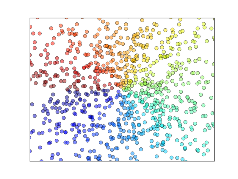
================================================
# View more python tutorials on my Youtube and Youku channel!!!
# Youtube video tutorial: https://www.youtube.com/channel/UCdyjiB5H8Pu7aDTNVXTTpcg
# Youku video tutorial: http://i.youku.com/pythontutorial
# 11 - bar
"""
Please note, this script is for python3+.
If you are using python2+, please modify it accordingly.
Tutorial reference:
http://www.scipy-lectures.org/intro/matplotlib/matplotlib.html
"""
import matplotlib.pyplot as plt
import numpy as np
n = 12
X = np.arange(n)
Y1 = (1 - X / float(n)) * np.random.uniform(0.5, 1.0, n)
Y2 = (1 - X / float(n)) * np.random.uniform(0.5, 1.0, n)
plt.bar(X, +Y1, facecolor='#9999ff', edgecolor='white')
plt.bar(X, -Y2, facecolor='#ff9999', edgecolor='white')
for x, y in zip(X, Y1):
# ha: horizontal alignment
# va: vertical alignment
plt.text(x + 0.4, y + 0.05, '%.2f' % y, ha='center', va='bottom')
for x, y in zip(X, Y2):
# ha: horizontal alignment
# va: vertical alignment
plt.text(x + 0.4, -y - 0.05, '%.2f' % y, ha='center', va='top')
plt.xlim(-.5, n)
plt.xticks(())
plt.ylim(-1.25, 1.25)
plt.yticks(())
plt.show()
================================================
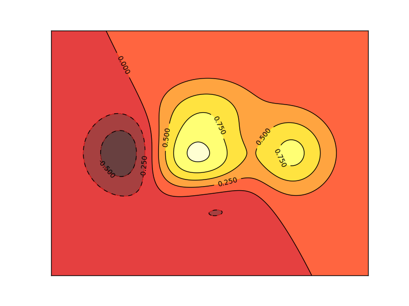
FILE: matplotlibTUT/plt12_contours.py
================================================
# View more python tutorials on my Youtube and Youku channel!!!
# Youtube video tutorial: https://www.youtube.com/channel/UCdyjiB5H8Pu7aDTNVXTTpcg
# Youku video tutorial: http://i.youku.com/pythontutorial
# 12 - contours
"""
Please note, this script is for python3+.
If you are using python2+, please modify it accordingly.
Tutorial reference:
http://www.scipy-lectures.org/intro/matplotlib/matplotlib.html
"""
import matplotlib.pyplot as plt
import numpy as np
def f(x,y):
# the height function
return (1 - x / 2 + x**5 + y**3) * np.exp(-x**2 -y**2)
n = 256
x = np.linspace(-3, 3, n)
y = np.linspace(-3, 3, n)
X,Y = np.meshgrid(x, y)
# use plt.contourf to filling contours
# X, Y and value for (X,Y) point
plt.contourf(X, Y, f(X, Y), 8, alpha=.75, cmap=plt.cm.hot)
# use plt.contour to add contour lines
C = plt.contour(X, Y, f(X, Y), 8, colors='black', linewidth=.5)
# adding label
plt.clabel(C, inline=True, fontsize=10)
plt.xticks(())
plt.yticks(())
plt.show()
================================================
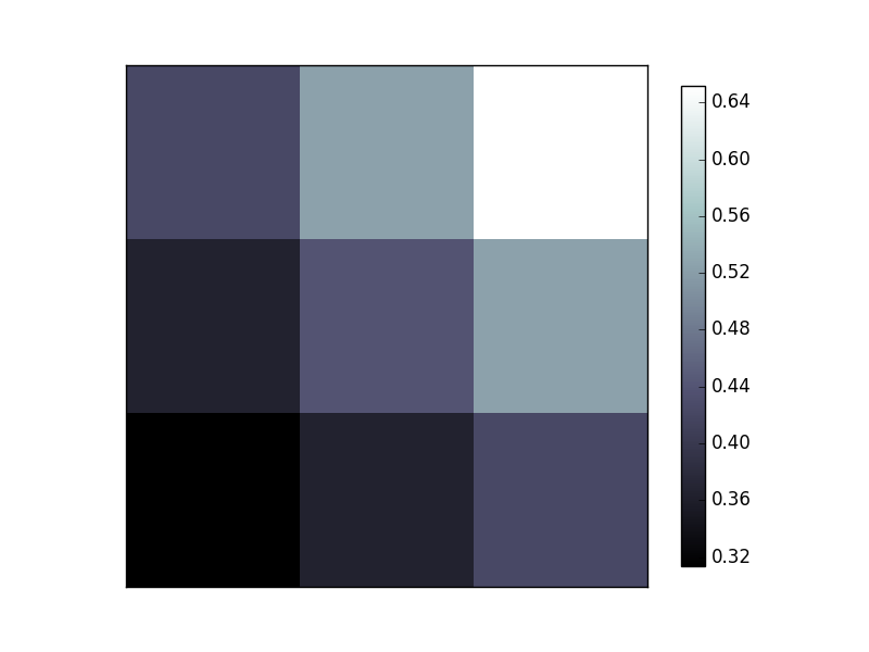
FILE: matplotlibTUT/plt13_image.py
================================================
# View more python tutorials on my Youtube and Youku channel!!!
# Youtube video tutorial: https://www.youtube.com/channel/UCdyjiB5H8Pu7aDTNVXTTpcg
# Youku video tutorial: http://i.youku.com/pythontutorial
# 13 - image
"""
Please note, this script is for python3+.
If you are using python2+, please modify it accordingly.
"""
import matplotlib.pyplot as plt
import numpy as np
# image data
a = np.array([0.313660827978, 0.365348418405, 0.423733120134,
0.365348418405, 0.439599930621, 0.525083754405,
0.423733120134, 0.525083754405, 0.651536351379]).reshape(3,3)
"""
for the value of "interpolation", check this:
http://matplotlib.org/examples/images_contours_and_fields/interpolation_methods.html
for the value of "origin"= ['upper', 'lower'], check this:
http://matplotlib.org/examples/pylab_examples/image_origin.html
"""
plt.imshow(a, interpolation='nearest', cmap='bone', origin='lower')
plt.colorbar(shrink=.92)
plt.xticks(())
plt.yticks(())
plt.show()
================================================
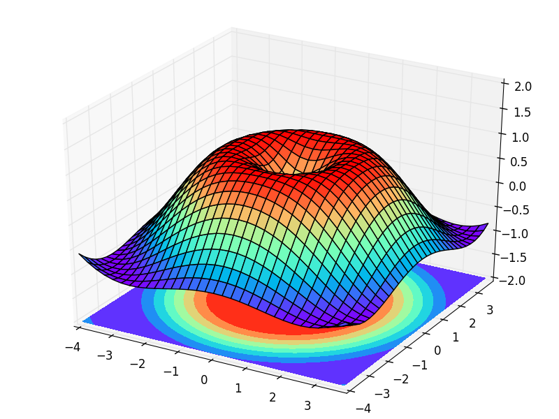
FILE: matplotlibTUT/plt14_3d.py
================================================
# View more python tutorials on my Youtube and Youku channel!!!
# Youtube video tutorial: https://www.youtube.com/channel/UCdyjiB5H8Pu7aDTNVXTTpcg
# Youku video tutorial: http://i.youku.com/pythontutorial
# 14 - 3d
"""
Please note, this script is for python3+.
If you are using python2+, please modify it accordingly.
Tutorial reference:
http://www.python-course.eu/matplotlib_multiple_figures.php
"""
import numpy as np
import matplotlib.pyplot as plt
from mpl_toolkits.mplot3d import Axes3D
fig = plt.figure()
ax = Axes3D(fig)
# X, Y value
X = np.arange(-4, 4, 0.25)
Y = np.arange(-4, 4, 0.25)
X, Y = np.meshgrid(X, Y)
R = np.sqrt(X ** 2 + Y ** 2)
# height value
Z = np.sin(R)
ax.plot_surface(X, Y, Z, rstride=1, cstride=1, cmap=plt.get_cmap('rainbow'))
"""
============= ================================================
Argument Description
============= ================================================
*X*, *Y*, *Z* Data values as 2D arrays
*rstride* Array row stride (step size), defaults to 10
*cstride* Array column stride (step size), defaults to 10
*color* Color of the surface patches
*cmap* A colormap for the surface patches.
*facecolors* Face colors for the individual patches
*norm* An instance of Normalize to map values to colors
*vmin* Minimum value to map
*vmax* Maximum value to map
*shade* Whether to shade the facecolors
============= ================================================
"""
# I think this is different from plt12_contours
ax.contourf(X, Y, Z, zdir='z', offset=-2, cmap=plt.get_cmap('rainbow'))
"""
========== ================================================
Argument Description
========== ================================================
*X*, *Y*, Data values as numpy.arrays
*Z*
*zdir* The direction to use: x, y or z (default)
*offset* If specified plot a projection of the filled contour
on this position in plane normal to zdir
========== ================================================
"""
ax.set_zlim(-2, 2)
plt.show()
================================================
FILE: matplotlibTUT/plt15_subplot.py
================================================
# View more python tutorials on my Youtube and Youku channel!!!
# Youtube video tutorial: https://www.youtube.com/channel/UCdyjiB5H8Pu7aDTNVXTTpcg
# Youku video tutorial: http://i.youku.com/pythontutorial
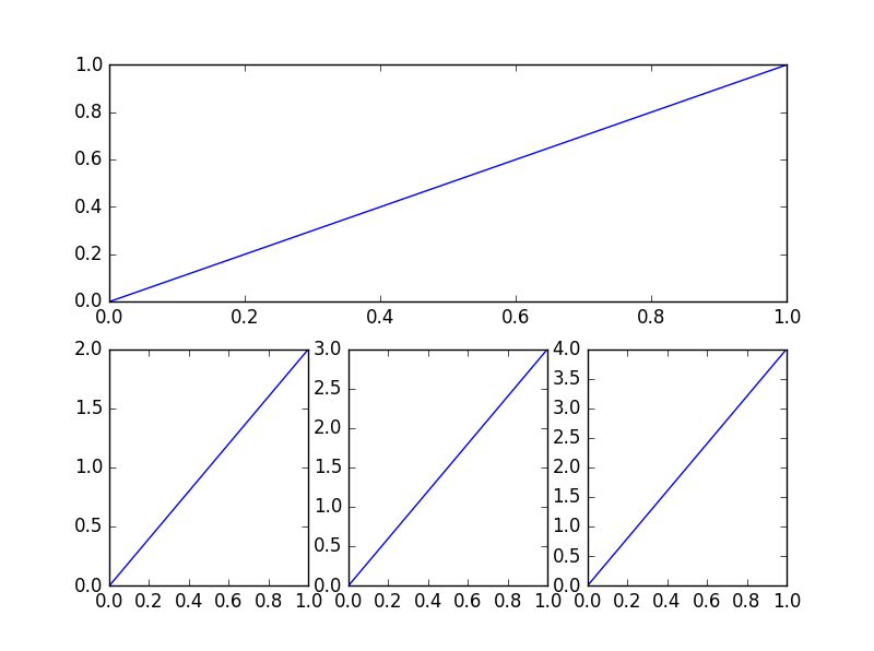
# 15 - subplot
"""
Please note, this script is for python3+.
If you are using python2+, please modify it accordingly.
Tutorial reference:
http://www.scipy-lectures.org/intro/matplotlib/matplotlib.html
"""
import matplotlib.pyplot as plt
# example 1:
###############################
plt.figure(figsize=(6, 4))
# plt.subplot(n_rows, n_cols, plot_num)
plt.subplot(2, 2, 1)
plt.plot([0, 1], [0, 1])
plt.subplot(222)
plt.plot([0, 1], [0, 2])
plt.subplot(223)
plt.plot([0, 1], [0, 3])
plt.subplot(224)
plt.plot([0, 1], [0, 4])
plt.tight_layout()
# example 2:
###############################
plt.figure(figsize=(6, 4))
# plt.subplot(n_rows, n_cols, plot_num)
plt.subplot(2, 1, 1)
# figure splits into 2 rows, 1 col, plot to the 1st sub-fig
plt.plot([0, 1], [0, 1])
plt.subplot(234)
# figure splits into 2 rows, 3 col, plot to the 4th sub-fig
plt.plot([0, 1], [0, 2])
plt.subplot(235)
# figure splits into 2 rows, 3 col, plot to the 5th sub-fig
plt.plot([0, 1], [0, 3])
plt.subplot(236)
# figure splits into 2 rows, 3 col, plot to the 6th sub-fig
plt.plot([0, 1], [0, 4])
plt.tight_layout()
plt.show()
================================================
FILE: matplotlibTUT/plt16_grid_subplot.py
================================================
# View more python tutorials on my Youtube and Youku channel!!!
# Youtube video tutorial: https://www.youtube.com/channel/UCdyjiB5H8Pu7aDTNVXTTpcg
# Youku video tutorial: http://i.youku.com/pythontutorial
# 16 - grid
"""
Please note, this script is for python3+.
If you are using python2+, please modify it accordingly.
Tutorial reference:
http://matplotlib.org/users/gridspec.html
"""
import matplotlib.pyplot as plt
import matplotlib.gridspec as gridspec
# method 1: subplot2grid
##########################
plt.figure()
ax1 = plt.subplot2grid((3, 3), (0, 0), colspan=3) # stands for axes
ax1.plot([1, 2], [1, 2])
ax1.set_title('ax1_title')
ax2 = plt.subplot2grid((3, 3), (1, 0), colspan=2)
ax3 = plt.subplot2grid((3, 3), (1, 2), rowspan=2)
ax4 = plt.subplot2grid((3, 3), (2, 0))
ax4.scatter([1, 2], [2, 2])
ax4.set_xlabel('ax4_x')
ax4.set_ylabel('ax4_y')
ax5 = plt.subplot2grid((3, 3), (2, 1))
# method 2: gridspec
#########################
plt.figure()
gs = gridspec.GridSpec(3, 3)
# use index from 0
ax6 = plt.subplot(gs[0, :])
ax7 = plt.subplot(gs[1, :2])
ax8 = plt.subplot(gs[1:, 2])
ax9 = plt.subplot(gs[-1, 0])
ax10 = plt.subplot(gs[-1, -2])
# method 3: easy to define structure
####################################
f, ((ax11, ax12), (ax13, ax14)) = plt.subplots(2, 2, sharex=True, sharey=True)
ax11.scatter([1,2], [1,2])
plt.tight_layout()
plt.show()
================================================
FILE: matplotlibTUT/plt17_plot_in_plot.py
================================================
# View more python tutorials on my Youtube and Youku channel!!!
# Youtube video tutorial: https://www.youtube.com/channel/UCdyjiB5H8Pu7aDTNVXTTpcg
# Youku video tutorial: http://i.youku.com/pythontutorial
# 17 - plot in plot
"""
Please note, this script is for python3+.
If you are using python2+, please modify it accordingly.
Tutorial reference:
http://www.python-course.eu/matplotlib_multiple_figures.php
"""
import matplotlib.pyplot as plt
fig = plt.figure()
x = [1, 2, 3, 4, 5, 6, 7]
y = [1, 3, 4, 2, 5, 8, 6]
# below are all percentage
left, bottom, width, height = 0.1, 0.1, 0.8, 0.8
ax1 = fig.add_axes([left, bottom, width, height]) # main axes
ax1.plot(x, y, 'r')
ax1.set_xlabel('x')
ax1.set_ylabel('y')
ax1.set_title('title')
ax2 = fig.add_axes([0.2, 0.6, 0.25, 0.25]) # inside axes
ax2.plot(y, x, 'b')
ax2.set_xlabel('x')
ax2.set_ylabel('y')
ax2.set_title('title inside 1')
# different method to add axes
####################################
plt.axes([0.6, 0.2, 0.25, 0.25])
plt.plot(y[::-1], x, 'g')
plt.xlabel('x')
plt.ylabel('y')
plt.title('title inside 2')
plt.show()
================================================
FILE: matplotlibTUT/plt18_secondary_yaxis.py
================================================
# View more python tutorials on my Youtube and Youku channel!!!
# Youtube video tutorial: https://www.youtube.com/channel/UCdyjiB5H8Pu7aDTNVXTTpcg
# Youku video tutorial: http://i.youku.com/pythontutorial
# 18 - secondary y axis
"""
Please note, this script is for python3+.
If you are using python2+, please modify it accordingly.
Tutorial reference:
http://www.python-course.eu/matplotlib_multiple_figures.php
"""
import matplotlib.pyplot as plt
import numpy as np
x = np.arange(0, 10, 0.1)
y1 = 0.05 * x**2
y2 = -1 *y1
fig, ax1 = plt.subplots()
ax2 = ax1.twinx() # mirror the ax1
ax1.plot(x, y1, 'g-')
ax2.plot(x, y2, 'b-')
ax1.set_xlabel('X data')
ax1.set_ylabel('Y1 data', color='g')
ax2.set_ylabel('Y2 data', color='b')
plt.show()
================================================
FILE: matplotlibTUT/plt19_animation.py
================================================
# View more python tutorials on my Youtube and Youku channel!!!
# Youtube video tutorial: https://www.youtube.com/channel/UCdyjiB5H8Pu7aDTNVXTTpcg
# Youku video tutorial: http://i.youku.com/pythontutorial
# 19 - animation
"""
Please note, this script is for python3+.
If you are using python2+, please modify it accordingly.
Tutorial reference:
http://matplotlib.org/examples/animation/simple_anim.html
More animation example code:
http://matplotlib.org/examples/animation/
"""
import numpy as np
from matplotlib import pyplot as plt
from matplotlib import animation
fig, ax = plt.subplots()
x = np.arange(0, 2*np.pi, 0.01)
line, = ax.plot(x, np.sin(x))
def animate(i):
line.set_ydata(np.sin(x + i/10.0)) # update the data
return line,
# Init only required for blitting to give a clean slate.
def init():
line.set_ydata(np.sin(x))
return line,
# call the animator. blit=True means only re-draw the parts that have changed.
# blit=True dose not work on Mac, set blit=False
# interval= update frequency
ani = animation.FuncAnimation(fig=fig, func=animate, frames=100, init_func=init,
interval=20, blit=False)
# save the animation as an mp4. This requires ffmpeg or mencoder to be
# installed. The extra_args ensure that the x264 codec is used, so that
# the video can be embedded in html5. You may need to adjust this for
# your system: for more information, see
# http://matplotlib.sourceforge.net/api/animation_api.html
# anim.save('basic_animation.mp4', fps=30, extra_args=['-vcodec', 'libx264'])
plt.show()
================================================
FILE: matplotlibTUT/plt1_why.py
================================================
# View more python tutorials on my Youtube and Youku channel!!!
# Youtube video tutorial: https://www.youtube.com/channel/UCdyjiB5H8Pu7aDTNVXTTpcg
# Youku video tutorial: http://i.youku.com/pythontutorial
# 1 - why
"""
1. matplotlib is a powerful python data visualization tool;
2. similar with MATLAB. If know matlab, easy to move over to python;
3. easy to plot 2D, 3D data;
4. you can even make animation.
"""
================================================
FILE: matplotlibTUT/plt2_install.py
================================================
# View more python tutorials on my Youtube and Youku channel!!!
# Youtube video tutorial: https://www.youtube.com/channel/UCdyjiB5H8Pu7aDTNVXTTpcg
# Youku video tutorial: http://i.youku.com/pythontutorial
# 2 - install
"""
Make sure you have installed numpy.
------------------------------
INSTALL on Linux:
If you have python3, in terminal you will type:
$ sudo apt-get install python3-matplotlib
Otherwise, if python2, type:
$ sudo apt-get install python-matplotlib
-------------------------------
INSTALL on MacOS
For python3:
$ pip3 install matplotlib
For python2:
$ pip install matplotlib
--------------------------------
INSTALL on Windows:
1. make sure you install Visual Studio;
2. go to: https://pypi.python.org/pypi/matplotlib/
3. find the wheel file (a file ending in .whl) matches your python version and system
(e.g. cp35 for python3.5, win32 for 32-bit system, win_amd64 for 64-bit system);
4. Copy the .whl file to your project folder, open a command window,
and navigate to the project folder. Then use pip to install matplotlib:
e.g.
> cd python_work
python_work> python -m pip3 install matplotlib-1.4.3-cp35-none-win32.whl
If not success. Try the alternative way: using "Anaconda" to install.
Please search this by yourself.
"""
================================================
FILE: matplotlibTUT/plt3_simple_plot.py
================================================
# View more python tutorials on my Youtube and Youku channel!!!
# Youtube video tutorial: https://www.youtube.com/channel/UCdyjiB5H8Pu7aDTNVXTTpcg
# Youku video tutorial: http://i.youku.com/pythontutorial
# 3 - simple plot
"""
Please note, this script is for python3+.
If you are using python2+, please modify it accordingly.
"""
import matplotlib.pyplot as plt
import numpy as np
x = np.linspace(-1, 1, 50)
y = 2*x + 1
# y = x**2
plt.plot(x, y)
plt.show()
================================================
FILE: matplotlibTUT/plt4_figure.py
================================================
# View more python tutorials on my Youtube and Youku channel!!!
# Youtube video tutorial: https://www.youtube.com/channel/UCdyjiB5H8Pu7aDTNVXTTpcg
# Youku video tutorial: http://i.youku.com/pythontutorial
# 4 - figure
"""
Please note, this script is for python3+.
If you are using python2+, please modify it accordingly.
Tutorial reference:
http://www.scipy-lectures.org/intro/matplotlib/matplotlib.html
"""
import matplotlib.pyplot as plt
import numpy as np
x = np.linspace(-3, 3, 50)
y1 = 2*x + 1
y2 = x**2
plt.figure()
plt.plot(x, y1)
plt.figure(num=3, figsize=(8, 5),)
plt.plot(x, y2)
# plot the second curve in this figure with certain parameters
plt.plot(x, y1, color='red', linewidth=1.0, linestyle='--')
plt.show()
================================================
FILE: matplotlibTUT/plt5_ax_setting1.py
================================================
# View more python tutorials on my Youtube and Youku channel!!!
# Youtube video tutorial: https://www.youtube.com/channel/UCdyjiB5H8Pu7aDTNVXTTpcg
# Youku video tutorial: http://i.youku.com/pythontutorial
# 5 - axis setting
"""
Please note, this script is for python3+.
If you are using python2+, please modify it accordingly.
Tutorial reference:
http://www.scipy-lectures.org/intro/matplotlib/matplotlib.html
"""
import matplotlib.pyplot as plt
import numpy as np
x = np.linspace(-3, 3, 50)
y1 = 2*x + 1
y2 = x**2
plt.figure()
plt.plot(x, y2)
# plot the second curve in this figure with certain parameters
plt.plot(x, y1, color='red', linewidth=1.0, linestyle='--')
# set x limits
plt.xlim((-1, 2))
plt.ylim((-2, 3))
plt.xlabel('I am x')
plt.ylabel('I am y')
# set new sticks
new_ticks = np.linspace(-1, 2, 5)
print(new_ticks)
plt.xticks(new_ticks)
# set tick labels
plt.yticks([-2, -1.8, -1, 1.22, 3],
[r'$really\ bad$', r'$bad$', r'$normal$', r'$good$', r'$really\ good$'])
plt.show()
================================================
FILE: matplotlibTUT/plt6_ax_setting2.py
================================================
# View more python tutorials on my Youtube and Youku channel!!!
# Youtube video tutorial: https://www.youtube.com/channel/UCdyjiB5H8Pu7aDTNVXTTpcg
# Youku video tutorial: http://i.youku.com/pythontutorial
# 6 - axis setting
"""
Please note, this script is for python3+.
If you are using python2+, please modify it accordingly.
Tutorial reference:
http://www.scipy-lectures.org/intro/matplotlib/matplotlib.html
"""
import matplotlib.pyplot as plt
import numpy as np
x = np.linspace(-3, 3, 50)
y1 = 2*x + 1
y2 = x**2
plt.figure()
plt.plot(x, y2)
# plot the second curve in this figure with certain parameters
plt.plot(x, y1, color='red', linewidth=1.0, linestyle='--')
# set x limits
plt.xlim((-1, 2))
plt.ylim((-2, 3))
# set new ticks
new_ticks = np.linspace(-1, 2, 5)
plt.xticks(new_ticks)
# set tick labels
plt.yticks([-2, -1.8, -1, 1.22, 3],
['$really\ bad$', '$bad$', '$normal$', '$good$', '$really\ good$'])
# to use '$ $' for math text and nice looking, e.g. '$\pi$'
# gca = 'get current axis'
ax = plt.gca()
ax.spines['right'].set_color('none')
ax.spines['top'].set_color('none')
ax.xaxis.set_ticks_position('bottom')
# ACCEPTS: [ 'top' | 'bottom' | 'both' | 'default' | 'none' ]
ax.spines['bottom'].set_position(('data', 0))
# the 1st is in 'outward' | 'axes' | 'data'
# axes: percentage of y axis
# data: depend on y data
ax.yaxis.set_ticks_position('left')
# ACCEPTS: [ 'left' | 'right' | 'both' | 'default' | 'none' ]
ax.spines['left'].set_position(('data',0))
plt.show()
================================================
FILE: matplotlibTUT/plt7_legend.py
================================================
# View more python tutorials on my Youtube and Youku channel!!!
# Youtube video tutorial: https://www.youtube.com/channel/UCdyjiB5H8Pu7aDTNVXTTpcg
# Youku video tutorial: http://i.youku.com/pythontutorial
# 7 - legend
"""
Please note, this script is for python3+.
If you are using python2+, please modify it accordingly.
Tutorial reference:
http://www.scipy-lectures.org/intro/matplotlib/matplotlib.html
"""
import matplotlib.pyplot as plt
import numpy as np
x = np.linspace(-3, 3, 50)
y1 = 2*x + 1
y2 = x**2
plt.figure()
# set x limits
plt.xlim((-1, 2))
plt.ylim((-2, 3))
# set new sticks
new_sticks = np.linspace(-1, 2, 5)
plt.xticks(new_sticks)
# set tick labels
plt.yticks([-2, -1.8, -1, 1.22, 3],
[r'$really\ bad$', r'$bad$', r'$normal$', r'$good$', r'$really\ good$'])
l1, = plt.plot(x, y1, label='linear line')
l2, = plt.plot(x, y2, color='red', linewidth=1.0, linestyle='--', label='square line')
plt.legend(loc='upper right')
# plt.legend(handles=[l1, l2], labels=['up', 'down'], loc='best')
# the "," is very important in here l1, = plt... and l2, = plt... for this step
"""legend( handles=(line1, line2, line3),
labels=('label1', 'label2', 'label3'),
'upper right')
The *loc* location codes are::
'best' : 0, (currently not supported for figure legends)
'upper right' : 1,
'upper left' : 2,
'lower left' : 3,
'lower right' : 4,
'right' : 5,
'center left' : 6,
'center right' : 7,
'lower center' : 8,
'upper center' : 9,
'center' : 10,"""
plt.show()
================================================
FILE: matplotlibTUT/plt8_annotation.py
================================================
# View more python tutorials on my Youtube and Youku channel!!!
# Youtube video tutorial: https://www.youtube.com/channel/UCdyjiB5H8Pu7aDTNVXTTpcg
# Youku video tutorial: http://i.youku.com/pythontutorial
# 8 - annotation
"""
Please note, this script is for python3+.
If you are using python2+, please modify it accordingly.
Tutorial reference:
http://www.scipy-lectures.org/intro/matplotlib/matplotlib.html
Mathematical expressions:
http://matplotlib.org/users/mathtext.html#mathtext-tutorial
"""
import matplotlib.pyplot as plt
import numpy as np
x = np.linspace(-3, 3, 50)
y = 2*x + 1
plt.figure(num=1, figsize=(8, 5),)
plt.plot(x, y,)
ax = plt.gca()
ax.spines['right'].set_color('none')
ax.spines['top'].set_color('none')
ax.spines['top'].set_color('none')
ax.xaxis.set_ticks_position('bottom')
ax.spines['bottom'].set_position(('data', 0))
ax.yaxis.set_ticks_position('left')
ax.spines['left'].set_position(('data', 0))
x0 = 1
y0 = 2*x0 + 1
plt.plot([x0, x0,], [0, y0,], 'k--', linewidth=2.5)
plt.scatter([x0, ], [y0, ], s=50, color='b')
# method 1:
#####################
plt.annotate(r'$2x+1=%s$' % y0, xy=(x0, y0), xycoords='data', xytext=(+30, -30),
textcoords='offset points', fontsize=16,
arrowprops=dict(arrowstyle='->', connectionstyle="arc3,rad=.2"))
# method 2:
########################
plt.text(-3.7, 3, r'$This\ is\ the\ some\ text. \mu\ \sigma_i\ \alpha_t$',
fontdict={'size': 16, 'color': 'r'})
plt.show()
================================================
FILE: matplotlibTUT/plt9_tick_visibility.py
================================================
# View more python tutorials on my Youtube and Youku channel!!!
# Youtube video tutorial: https://www.youtube.com/channel/UCdyjiB5H8Pu7aDTNVXTTpcg
# Youku video tutorial: http://i.youku.com/pythontutorial
# 9 - tick_visibility
"""
Please note, this script is for python3+.
If you are using python2+, please modify it accordingly.
Tutorial reference:
http://www.scipy-lectures.org/intro/matplotlib/matplotlib.html
"""
import matplotlib.pyplot as plt
import numpy as np
x = np.linspace(-3, 3, 50)
y = 0.1*x
plt.figure()
plt.plot(x, y, linewidth=10, zorder=1) # set zorder for ordering the plot in plt 2.0.2 or higher
plt.ylim(-2, 2)
ax = plt.gca()
ax.spines['right'].set_color('none')
ax.spines['top'].set_color('none')
ax.spines['top'].set_color('none')
ax.xaxis.set_ticks_position('bottom')
ax.spines['bottom'].set_position(('data', 0))
ax.yaxis.set_ticks_position('left')
ax.spines['left'].set_position(('data', 0))
for label in ax.get_xticklabels() + ax.get_yticklabels():
label.set_fontsize(12)
# set zorder for ordering the plot in plt 2.0.2 or higher
label.set_bbox(dict(facecolor='white', edgecolor='none', alpha=0.8, zorder=2))
plt.show()
================================================
FILE: multiprocessingTUT/multiprocessing3_queue.py
================================================
# View more python learning tutorial on my Youtube and Youku channel!!!
# Youtube video tutorial: https://www.youtube.com/channel/UCdyjiB5H8Pu7aDTNVXTTpcg
# Youku video tutorial: http://i.youku.com/pythontutorial
import multiprocessing as mp
def job(q):
res = 0
for i in range(1000):
res += i+i**2+i**3
q.put(res) # queue
if __name__ == '__main__':
q = mp.Queue()
p1 = mp.Process(target=job, args=(q,))
p2 = mp.Process(target=job, args=(q,))
p1.start()
p2.start()
p1.join()
p2.join()
res1 = q.get()
res2 = q.get()
print(res1+res2)
================================================
FILE: multiprocessingTUT/multiprocessing4_efficiency_comparison.py
================================================
# View more python learning tutorial on my Youtube and Youku channel!!!
# Youtube video tutorial: https://www.youtube.com/channel/UCdyjiB5H8Pu7aDTNVXTTpcg
# Youku video tutorial: http://i.youku.com/pythontutorial
import multiprocessing as mp
import threading as td
import time
def job(q):
res = 0
for i in range(1000000):
res += i+i**2+i**3
q.put(res) # queue
def multicore():
q = mp.Queue()
p1 = mp.Process(target=job, args=(q,))
p2 = mp.Process(target=job, args=(q,))
p1.start()
p2.start()
p1.join()
p2.join()
res1 = q.get()
res2 = q.get()
print('multicore:' , res1+res2)
def normal():
res = 0
for _ in range(2):
for i in range(1000000):
res += i+i**2+i**3
print('normal:', res)
def multithread():
q = mp.Queue()
t1 = td.Thread(target=job, args=(q,))
t2 = td.Thread(target=job, args=(q,))
t1.start()
t2.start()
t1.join()
t2.join()
res1 = q.get()
res2 = q.get()
print('multithread:', res1+res2)
if __name__ == '__main__':
st = time.time()
normal()
st1= time.time()
print('normal time:', st1 - st)
multithread()
st2 = time.time()
print('multithread time:', st2 - st1)
multicore()
print('multicore time:', time.time()-st2)
================================================
FILE: multiprocessingTUT/multiprocessing5_pool.py
================================================
# View more python learning tutorial on my Youtube and Youku channel!!!
# Youtube video tutorial: https://www.youtube.com/channel/UCdyjiB5H8Pu7aDTNVXTTpcg
# Youku video tutorial: http://i.youku.com/pythontutorial
import multiprocessing as mp
def job(x):
return x*x
def multicore():
pool = mp.Pool(processes=2)
res = pool.map(job, range(10))
print(res)
res = pool.apply_async(job, (2,))
print(res.get())
multi_res =[pool.apply_async(job, (i,)) for i in range(10)]
print([res.get() for res in multi_res])
if __name__ == '__main__':
multicore()
================================================
FILE: multiprocessingTUT/multiprocessing7_lock.py
================================================
# View more python learning tutorial on my Youtube and Youku channel!!!
# Youtube video tutorial: https://www.youtube.com/channel/UCdyjiB5H8Pu7aDTNVXTTpcg
# Youku video tutorial: http://i.youku.com/pythontutorial
import multiprocessing as mp
import time
def job(v, num, l):
l.acquire()
for _ in range(10):
time.sleep(0.1)
v.value += num
print(v.value)
l.release()
def multicore():
l = mp.Lock()
v = mp.Value('i', 0)
p1 = mp.Process(target=job, args=(v, 1, l))
p2 = mp.Process(target=job, args=(v, 3, l))
p1.start()
p2.start()
p1.join()
p2.join()
if __name__ == '__main__':
multicore()
================================================
FILE: numpy&pandas/11_pandas_intro.py
================================================
# View more python tutorials on my Youtube and Youku channel!!!
# Youtube video tutorial: https://www.youtube.com/channel/UCdyjiB5H8Pu7aDTNVXTTpcg
# Youku video tutorial: http://i.youku.com/pythontutorial
"""
Please note, this code is only for python 3+. If you are using python 2+, please modify the code accordingly.
"""
from __future__ import print_function
import pandas as pd
import numpy as np
s = pd.Series([1,3,6,np.nan,4,1]) # similar with 1D numpy
print(s)
dates = pd.date_range('20160101', periods=6)
df = pd.DataFrame(np.random.randn(6,4), index=dates, columns=['A','B','C','D'])
print(df['B'])
df2 = pd.DataFrame({'A' : 1.,
'B' : pd.Timestamp('20130102'),
'C' : pd.Series(1,index=list(range(4)),dtype='float32'),
'D' : np.array([3] * 4,dtype='int32'),
'E' : pd.Categorical(["test","train","test","train"]),
'F' : 'foo'})
print(df2)
print(df2.dtypes)
print(df.index)
print(df.columns)
print(df.values)
print(df.describe())
print(df.T)
print(df.sort_index(axis=1, ascending=False))
print(df.sort_values(by='B'))
================================================
FILE: numpy&pandas/12_selection.py
================================================
# View more python tutorials on my Youtube and Youku channel!!!
# Youtube video tutorial: https://www.youtube.com/channel/UCdyjiB5H8Pu7aDTNVXTTpcg
# Youku video tutorial: http://i.youku.com/pythontutorial
"""
Please note, this code is only for python 3+. If you are using python 2+, please modify the code accordingly.
"""
from __future__ import print_function
import pandas as pd
import numpy as np
dates = pd.date_range('20130101', periods=6)
df = pd.DataFrame(np.random.randn(6,4), index=dates, columns=['A', 'B', 'C', 'D'])
print(df['A'], df.A)
print(df[0:3], df['20130102':'20130104'])
# select by label: loc
print(df.loc['20130102'])
print(df.loc[:,['A','B']])
print(df.loc['20130102', ['A','B']])
# select by position: iloc
print(df.iloc[3])
print(df.iloc[3, 1])
print(df.iloc[3:5,0:2])
print(df.iloc[[1,2,4],[0,2]])
# mixed selection: ix
print(df.ix[:3, ['A', 'C']])
# Boolean indexing
print(df[df.A > 0])
================================================
FILE: numpy&pandas/13_set_value.py
================================================
# View more python tutorials on my Youtube and Youku channel!!!
# Youtube video tutorial: https://www.youtube.com/channel/UCdyjiB5H8Pu7aDTNVXTTpcg
# Youku video tutorial: http://i.youku.com/pythontutorial
"""
Please note, this code is only for python 3+. If you are using python 2+, please modify the code accordingly.
"""
from __future__ import print_function
import pandas as pd
import numpy as np
dates = pd.date_range('20130101', periods=6)
df = pd.DataFrame(np.random.randn(6,4), index=dates, columns=['A', 'B', 'C', 'D'])
df.iloc[2,2] = 1111
df.loc['2013-01-03', 'D'] = 2222
df.A[df.A>0] = 0
df['F'] = np.nan
df['G'] = pd.Series([1,2,3,4,5,6], index=pd.date_range('20130101', periods=6))
print(df)
================================================
FILE: numpy&pandas/14_nan.py
================================================
# View more python tutorials on my Youtube and Youku channel!!!
# Youtube video tutorial: https://www.youtube.com/channel/UCdyjiB5H8Pu7aDTNVXTTpcg
# Youku video tutorial: http://i.youku.com/pythontutorial
"""
Please note, this code is only for python 3+. If you are using python 2+, please modify the code accordingly.
"""
from __future__ import print_function
import pandas as pd
import numpy as np
dates = pd.date_range('20130101', periods=6)
df = pd.DataFrame(np.arange(24).reshape((6,4)), index=dates, columns=['A', 'B', 'C', 'D'])
df.iloc[0,1] = np.nan
df.iloc[1,2] = np.nan
print(df.dropna(axis=0, how='any')) # how={'any', 'all'}
print(df.fillna(value=0))
print(pd.isnull(df))
================================================
FILE: numpy&pandas/15_read_to/15_read_to.py
================================================
# View more python tutorials on my Youtube and Youku channel!!!
# Youtube video tutorial: https://www.youtube.com/channel/UCdyjiB5H8Pu7aDTNVXTTpcg
# Youku video tutorial: http://i.youku.com/pythontutorial
"""
Please note, this code is only for python 3+. If you are using python 2+, please modify the code accordingly.
"""
from __future__ import print_function
import pandas as pd
# read from
data = pd.read_csv('student.csv')
print(data)
# save to
data.to_pickle('student.pickle')
================================================
FILE: numpy&pandas/15_read_to/student.csv
================================================
Student ID,name ,age,gender
1100,Kelly,22,Female
1101,Clo,21,Female
1102,Tilly,22,Female
1103,Tony,24,Male
1104,David,20,Male
1105,Catty,22,Female
1106,M,3,Female
1107,N,43,Male
1108,A,13,Male
1109,S,12,Male
1110,David,33,Male
1111,Dw,3,Female
1112,Q,23,Male
1113,W,21,Female
================================================
FILE: numpy&pandas/16_concat.py
================================================
# View more python tutorials on my Youtube and Youku channel!!!
# Youtube video tutorial: https://www.youtube.com/channel/UCdyjiB5H8Pu7aDTNVXTTpcg
# Youku video tutorial: http://i.youku.com/pythontutorial
"""
Please note, this code is only for python 3+. If you are using python 2+, please modify the code accordingly.
"""
from __future__ import print_function
import pandas as pd
import numpy as np
# concatenating
# ignore index
df1 = pd.DataFrame(np.ones((3,4))*0, columns=['a','b','c','d'])
df2 = pd.DataFrame(np.ones((3,4))*1, columns=['a','b','c','d'])
df3 = pd.DataFrame(np.ones((3,4))*2, columns=['a','b','c','d'])
res = pd.concat([df1, df2, df3], axis=0, ignore_index=True)
# join, ('inner', 'outer')
df1 = pd.DataFrame(np.ones((3,4))*0, columns=['a','b','c','d'], index=[1,2,3])
df2 = pd.DataFrame(np.ones((3,4))*1, columns=['b','c','d', 'e'], index=[2,3,4])
res = pd.concat([df1, df2], axis=1, join='outer')
res = pd.concat([df1, df2], axis=1, join='inner')
# join_axes
res = pd.concat([df1, df2], axis=1, join_axes=[df1.index])
# append
df1 = pd.DataFrame(np.ones((3,4))*0, columns=['a','b','c','d'])
df2 = pd.DataFrame(np.ones((3,4))*1, columns=['a','b','c','d'])
df2 = pd.DataFrame(np.ones((3,4))*1, columns=['b','c','d', 'e'], index=[2,3,4])
res = df1.append(df2, ignore_index=True)
res = df1.append([df2, df3])
s1 = pd.Series([1,2,3,4], index=['a','b','c','d'])
res = df1.append(s1, ignore_index=True)
print(res)
================================================
FILE: numpy&pandas/17_merge.py
================================================
# View more python tutorials on my Youtube and Youku channel!!!
# Youtube video tutorial: https://www.youtube.com/channel/UCdyjiB5H8Pu7aDTNVXTTpcg
# Youku video tutorial: http://i.youku.com/pythontutorial
"""
Please note, this code is only for python 3+. If you are using python 2+, please modify the code accordingly.
"""
from __future__ import print_function
import pandas as pd
# merging two df by key/keys. (may be used in database)
# simple example
left = pd.DataFrame({'key': ['K0', 'K1', 'K2', 'K3'],
'A': ['A0', 'A1', 'A2', 'A3'],
'B': ['B0', 'B1', 'B2', 'B3']})
right = pd.DataFrame({'key': ['K0', 'K1', 'K2', 'K3'],
'C': ['C0', 'C1', 'C2', 'C3'],
'D': ['D0', 'D1', 'D2', 'D3']})
print(left)
print(right)
res = pd.merge(left, right, on='key')
print(res)
# consider two keys
left = pd.DataFrame({'key1': ['K0', 'K0', 'K1', 'K2'],
'key2': ['K0', 'K1', 'K0', 'K1'],
'A': ['A0', 'A1', 'A2', 'A3'],
'B': ['B0', 'B1', 'B2', 'B3']})
right = pd.DataFrame({'key1': ['K0', 'K1', 'K1', 'K2'],
'key2': ['K0', 'K0', 'K0', 'K0'],
'C': ['C0', 'C1', 'C2', 'C3'],
'D': ['D0', 'D1', 'D2', 'D3']})
print(left)
print(right)
res = pd.merge(left, right, on=['key1', 'key2'], how='inner') # default for how='inner'
# how = ['left', 'right', 'outer', 'inner']
res = pd.merge(left, right, on=['key1', 'key2'], how='left')
print(res)
# indicator
df1 = pd.DataFrame({'col1':[0,1], 'col_left':['a','b']})
df2 = pd.DataFrame({'col1':[1,2,2],'col_right':[2,2,2]})
print(df1)
print(df2)
res = pd.merge(df1, df2, on='col1', how='outer', indicator=True)
# give the indicator a custom name
res = pd.merge(df1, df2, on='col1', how='outer', indicator='indicator_column')
# merged by index
left = pd.DataFrame({'A': ['A0', 'A1', 'A2'],
'B': ['B0', 'B1', 'B2']},
index=['K0', 'K1', 'K2'])
right = pd.DataFrame({'C': ['C0', 'C2', 'C3'],
'D': ['D0', 'D2', 'D3']},
index=['K0', 'K2', 'K3'])
print(left)
print(right)
# left_index and right_index
res = pd.merge(left, right, left_index=True, right_index=True, how='outer')
res = pd.merge(left, right, left_index=True, right_index=True, how='inner')
# handle overlapping
boys = pd.DataFrame({'k': ['K0', 'K1', 'K2'], 'age': [1, 2, 3]})
girls = pd.DataFrame({'k': ['K0', 'K0', 'K3'], 'age': [4, 5, 6]})
res = pd.merge(boys, girls, on='k', suffixes=['_boy', '_girl'], how='inner')
print(res)
# join function in pandas is similar with merge. If know merge, you will understand join
================================================
FILE: numpy&pandas/18_plot.py
================================================
# View more python tutorials on my Youtube and Youku channel!!!
# Youtube video tutorial: https://www.youtube.com/channel/UCdyjiB5H8Pu7aDTNVXTTpcg
# Youku video tutorial: http://i.youku.com/pythontutorial
"""
Please note, this code is only for python 3+. If you are using python 2+, please modify the code accordingly.
"""
from __future__ import print_function
import pandas as pd
import numpy as np
import matplotlib.pyplot as plt
# plot data
# Series
data = pd.Series(np.random.randn(1000), index=np.arange(1000))
data = data.cumsum()
##data.plot()
# DataFrame
data = pd.DataFrame(np.random.randn(1000, 4), index=np.arange(1000), columns=list("ABCD"))
data = data.cumsum()
# plot methods:
# 'bar', 'hist', 'box', 'kde', 'area', scatter', hexbin', 'pie'
ax = data.plot.scatter(x='A', y='B', color='DarkBlue', label="Class 1")
data.plot.scatter(x='A', y='C', color='LightGreen', label='Class 2', ax=ax)
plt.show()
================================================
FILE: pyTorch tutorial/README.md
================================================

---
# This pyTorch Tutorial has been moved to anther independent repo:
[/MorvanZhou/PyTorch-Tutorial](/MorvanZhou/PyTorch-Tutorial)
# 请注意, 这个 PyTorch 的教程代码已经被移至另一个网页:
[/MorvanZhou/PyTorch-Tutorial](/MorvanZhou/PyTorch-Tutorial)
# Donation
*If this does help you, please consider donating to support me for better tutorials. Any contribution is greatly appreciated!*
================================================
FILE: sklearnTUT/sk10_cross_validation3.py
================================================
# View more python learning tutorial on my Youtube and Youku channel!!!
# Youtube video tutorial: https://www.youtube.com/channel/UCdyjiB5H8Pu7aDTNVXTTpcg
# Youku video tutorial: http://i.youku.com/pythontutorial
"""
Please note, this code is only for python 3+. If you are using python 2+, please modify the code accordingly.
"""
from __future__ import print_function
from sklearn.learning_curve import validation_curve
from sklearn.datasets import load_digits
from sklearn.svm import SVC
import matplotlib.pyplot as plt
import numpy as np
digits = load_digits()
X = digits.data
y = digits.target
param_range = np.logspace(-6, -2.3, 5)
train_loss, test_loss = validation_curve(
SVC(), X, y, param_name='gamma', param_range=param_range, cv=10,
scoring='mean_squared_error')
train_loss_mean = -np.mean(train_loss, axis=1)
test_loss_mean = -np.mean(test_loss, axis=1)
plt.plot(param_range, train_loss_mean, 'o-', color="r",
label="Training")
plt.plot(param_range, test_loss_mean, 'o-', color="g",
label="Cross-validation")
plt.xlabel("gamma")
plt.ylabel("Loss")
plt.legend(loc="best")
plt.show()
================================================
FILE: sklearnTUT/sk11_save.py
================================================
# View more python tutorials on my Youtube and Youku channel!!!
# Youtube video tutorial: https://www.youtube.com/channel/UCdyjiB5H8Pu7aDTNVXTTpcg
# Youku video tutorial: http://i.youku.com/pythontutorial
"""
Please note, this code is only for python 3+. If you are using python 2+, please modify the code accordingly.
"""
from __future__ import print_function
from sklearn import svm
from sklearn import datasets
clf = svm.SVC()
iris = datasets.load_iris()
X, y = iris.data, iris.target
clf.fit(X, y)
# method 1: pickle
import pickle
# save
with open('save/clf.pickle', 'wb') as f:
pickle.dump(clf, f)
# restore
with open('save/clf.pickle', 'rb') as f:
clf2 = pickle.load(f)
print(clf2.predict(X[0:1]))
# method 2: joblib
from sklearn.externals import joblib
# Save
joblib.dump(clf, 'save/clf.pkl')
# restore
clf3 = joblib.load('save/clf.pkl')
print(clf3.predict(X[0:1]))
================================================
FILE: sklearnTUT/sk4_learning_pattern.py
================================================
# View more python learning tutorial on my Youtube and Youku channel!!!
# Youtube video tutorial: https://www.youtube.com/channel/UCdyjiB5H8Pu7aDTNVXTTpcg
# Youku video tutorial: http://i.youku.com/pythontutorial
"""
Please note, this code is only for python 3+. If you are using python 2+, please modify the code accordingly.
"""
from __future__ import print_function
from sklearn import datasets
from sklearn.model_selection import train_test_split
from sklearn.neighbors import KNeighborsClassifier
iris = datasets.load_iris()
iris_X = iris.data
iris_y = iris.target
##print(iris_X[:2, :])
##print(iris_y)
X_train, X_test, y_train, y_test = train_test_split(
iris_X, iris_y, test_size=0.3)
##print(y_train)
knn = KNeighborsClassifier()
knn.fit(X_train, y_train)
print(knn.predict(X_test))
print(y_test)
================================================
FILE: sklearnTUT/sk5_datasets.py
================================================
# View more python learning tutorial on my Youtube and Youku channel!!!
# Youtube video tutorial: https://www.youtube.com/channel/UCdyjiB5H8Pu7aDTNVXTTpcg
# Youku video tutorial: http://i.youku.com/pythontutorial
"""
Please note, this code is only for python 3+. If you are using python 2+, please modify the code accordingly.
"""
from __future__ import print_function
from sklearn import datasets
from sklearn.linear_model import LinearRegression
import matplotlib.pyplot as plt
loaded_data = datasets.load_boston()
data_X = loaded_data.data
data_y = loaded_data.target
model = LinearRegression()
model.fit(data_X, data_y)
print(model.predict(data_X[:4, :]))
print(data_y[:4])
X, y = datasets.make_regression(n_samples=100, n_features=1, n_targets=1, noise=10)
plt.scatter(X, y)
plt.show()
================================================
FILE: sklearnTUT/sk6_model_attribute_method.py
================================================
# View more python learning tutorial on my Youtube and Youku channel!!!
# Youtube video tutorial: https://www.youtube.com/channel/UCdyjiB5H8Pu7aDTNVXTTpcg
# Youku video tutorial: http://i.youku.com/pythontutorial
"""
Please note, this code is only for python 3+. If you are using python 2+, please modify the code accordingly.
"""
from __future__ import print_function
from sklearn import datasets
from sklearn.linear_model import LinearRegression
loaded_data = datasets.load_boston()
data_X = loaded_data.data
data_y = loaded_data.target
model = LinearRegression()
model.fit(data_X, data_y)
print(model.predict(data_X[:4, :]))
print(model.coef_)
print(model.intercept_)
print(model.get_params())
print(model.score(data_X, data_y)) # R^2 coefficient of determination
================================================
FILE: sklearnTUT/sk7_normalization.py
================================================
# View more python learning tutorial on my Youtube and Youku channel!!!
# Youtube video tutorial: https://www.youtube.com/channel/UCdyjiB5H8Pu7aDTNVXTTpcg
# Youku video tutorial: http://i.youku.com/pythontutorial
"""
Please note, this code is only for python 3+. If you are using python 2+, please modify the code accordingly.
"""
from __future__ import print_function
from sklearn import preprocessing
import numpy as np
from sklearn.model_selection import train_test_split
from sklearn.datasets.samples_generator import make_classification
from sklearn.svm import SVC
import matplotlib.pyplot as plt
a = np.array([[10, 2.7, 3.6],
[-100, 5, -2],
[120, 20, 40]], dtype=np.float64)
print(a)
print(preprocessing.scale(a))
X, y = make_classification(n_samples=300, n_features=2 , n_redundant=0, n_informative=2,
random_state=22, n_clusters_per_class=1, scale=100)
plt.scatter(X[:, 0], X[:, 1], c=y)
plt.show()
X = preprocessing.scale(X) # normalization step
X_train, X_test, y_train, y_test = train_test_split(X, y, test_size=.3)
clf = SVC()
clf.fit(X_train, y_train)
print(clf.score(X_test, y_test))
================================================
FILE: sklearnTUT/sk8_cross_validation/for_you_to_practice.py
================================================
# View more python learning tutorial on my Youtube and Youku channel!!!
# Youtube video tutorial: https://www.youtube.com/channel/UCdyjiB5H8Pu7aDTNVXTTpcg
# Youku video tutorial: http://i.youku.com/pythontutorial
"""
Please note, this code is only for python 3+. If you are using python 2+, please modify the code accordingly.
"""
from __future__ import print_function
from sklearn.datasets import load_iris
from sklearn.cross_validation import train_test_split
from sklearn.neighbors import KNeighborsClassifier
iris = load_iris()
X = iris.data
y = iris.target
# test train split #
# this is cross_val_score #
# this is how to use cross_val_score to choose model and configs #
================================================
FILE: sklearnTUT/sk8_cross_validation/full_code.py
================================================
# View more python learning tutorial on my Youtube and Youku channel!!!
# Youtube video tutorial: https://www.youtube.com/channel/UCdyjiB5H8Pu7aDTNVXTTpcg
# Youku video tutorial: http://i.youku.com/pythontutorial
"""
Please note, this code is only for python 3+. If you are using python 2+, please modify the code accordingly.
"""
from __future__ import print_function
from sklearn.datasets import load_iris
from sklearn.cross_validation import train_test_split
from sklearn.neighbors import KNeighborsClassifier
iris = load_iris()
X = iris.data
y = iris.target
# test train split #
X_train, X_test, y_train, y_test = train_test_split(X, y, random_state=4)
knn = KNeighborsClassifier(n_neighbors=5)
knn.fit(X_train, y_train)
y_pred = knn.predict(X_test)
print(knn.score(X_test, y_test))
# this is cross_val_score #
from sklearn.cross_validation import cross_val_score
knn = KNeighborsClassifier(n_neighbors=5)
scores = cross_val_score(knn, X, y, cv=5, scoring='accuracy')
print(scores)
# this is how to use cross_val_score to choose model and configs #
from sklearn.cross_validation import cross_val_score
import matplotlib.pyplot as plt
k_range = range(1, 31)
k_scores = []
for k in k_range:
knn = KNeighborsClassifier(n_neighbors=k)
## loss = -cross_val_score(knn, X, y, cv=10, scoring='mean_squared_error') # for regression
scores = cross_val_score(knn, X, y, cv=10, scoring='accuracy') # for classification
k_scores.append(scores.mean())
plt.plot(k_range, k_scores)
plt.xlabel('Value of K for KNN')
plt.ylabel('Cross-Validated Accuracy')
plt.show()
================================================
FILE: sklearnTUT/sk9_cross_validation2.py
================================================
# View more python learning tutorial on my Youtube and Youku channel!!!
# Youtube video tutorial: https://www.youtube.com/channel/UCdyjiB5H8Pu7aDTNVXTTpcg
# Youku video tutorial: http://i.youku.com/pythontutorial
"""
Please note, this code is only for python 3+. If you are using python 2+, please modify the code accordingly.
"""
from __future__ import print_function
from sklearn.learning_curve import learning_curve
from sklearn.datasets import load_digits
from sklearn.svm import SVC
import matplotlib.pyplot as plt
import numpy as np
digits = load_digits()
X = digits.data
y = digits.target
train_sizes, train_loss, test_loss= learning_curve(
SVC(gamma=0.01), X, y, cv=10, scoring='mean_squared_error',
train_sizes=[0.1, 0.25, 0.5, 0.75, 1])
train_loss_mean = -np.mean(train_loss, axis=1)
test_loss_mean = -np.mean(test_loss, axis=1)
plt.plot(train_sizes, train_loss_mean, 'o-', color="r",
label="Training")
plt.plot(train_sizes, test_loss_mean, 'o-', color="g",
label="Cross-validation")
plt.xlabel("Training examples")
plt.ylabel("Loss")
plt.legend(loc="best")
plt.show()
================================================
FILE: tensorflowTUT/README.md
================================================

---
### This tutorial codes are old, so I made a [new series of Tensorflow tutorial](https://github.com/MorvanZhou/Tensorflow-Tutorial). In the new tutorials, codes are updated, contents are better organized. If you like that, please star it!
# Tensorflow Tutorials
In these tutorials for Tensorflow, we will build our first Neural Network and try to build some advanced Neural Network architectures developed recent years.
All methods mentioned below have their video and text tutorial in Chinese. Visit [莫烦 Python](https://mofanpy.com/tutorials/) for more.
If you speak Chinese, you can watch my [Youtube channel](https://www.youtube.com/channel/UCdyjiB5H8Pu7aDTNVXTTpcg) as well.
**As many requests about making these tutorials available in English, please find them in this playlist:** ([https://www.youtube.com/playlist?list=PLXO45tsB95cJHXaDKpbwr5fC_CCYylw1f](https://www.youtube.com/playlist?list=PLXO45tsB95cJHXaDKpbwr5fC_CCYylw1f))
* Tensorflow Basic
* [Basic example](tf5_example2/full_code.py)
* [Session](tensorflow6_session.py)
* [Variable](tensorflow7_variable.py)
* [Placeholder](tensorflow8_feeds.py)
* Build your first NN
* [Adding layer](tensorflow10_def_add_layer.py)
* [Build NN](tf11_build_network/full_code.py)
* [Visualize update](tf12_plot_result/full_code.py)
* Tensorboard
* [Visualization 1](tf14_tensorboard/full_code.py)
* [Visualization 2](tf15_tensorboard/full_code.py)
* [Classification](tf16_classification/full_code.py)
* [Overfitting and dropout](tf17_dropout/full_code.py)
* [Save Network](tf19_saver.py)
* CNN
* [CNN layers](tf18_CNN2/full_code.py)
* [CNN training](tf18_CNN3/full_code.py)
* RNN
* [Classification](tf20_RNN2/full_code.py)
* [Regression](tf20_RNN2.2/full_code.py)
* [Autoencoder](tf21_autoencoder/full_code.py)
* Scope
* [Scope in TF](tf22_scope/tf22_scope.py)
* [Training Testing for RNN](tf22_scope/tf22_RNN_scope.py)
* [Batch Normalization](tf23_BN/tf23_BN.py)
# Donation
*If this does help you, please consider donating to support me for better tutorials. Any contribution is greatly appreciated!*
================================================
FILE: tensorflowTUT/tensorflow10_def_add_layer.py
================================================
# View more python learning tutorial on my Youtube and Youku channel!!!
# Youtube video tutorial: https://www.youtube.com/channel/UCdyjiB5H8Pu7aDTNVXTTpcg
# Youku video tutorial: http://i.youku.com/pythontutorial
"""
Please note, this code is only for python 3+. If you are using python 2+, please modify the code accordingly.
"""
from __future__ import print_function
import tensorflow as tf
def add_layer(inputs, in_size, out_size, activation_function=None):
Weights = tf.Variable(tf.random_normal([in_size, out_size]))
biases = tf.Variable(tf.zeros([1, out_size]) + 0.1)
Wx_plus_b = tf.matmul(inputs, Weights) + biases
if activation_function is None:
outputs = Wx_plus_b
else:
outputs = activation_function(Wx_plus_b)
return outputs
================================================
FILE: tensorflowTUT/tensorflow11_build_network.py
================================================
# View more python learning tutorial on my Youtube and Youku channel!!!
# Youtube video tutorial: https://www.youtube.com/channel/UCdyjiB5H8Pu7aDTNVXTTpcg
# Youku video tutorial: http://i.youku.com/pythontutorial
"""
Please note, this code is only for python 3+. If you are using python 2+, please modify the code accordingly.
"""
from __future__ import print_function
import tensorflow as tf
import numpy as np
def add_layer(inputs, in_size, out_size, activation_function=None):
# add one more layer and return the output of this layer
Weights = tf.Variable(tf.random_normal([in_size, out_size]))
biases = tf.Variable(tf.zeros([1, out_size]) + 0.1)
Wx_plus_b = tf.matmul(inputs, Weights) + biases
if activation_function is None:
outputs = Wx_plus_b
else:
outputs = activation_function(Wx_plus_b)
return outputs
# Make up some real data
x_data = np.linspace(-1,1,300)[:, np.newaxis]
noise = np.random.normal(0, 0.05, x_data.shape)
y_data = np.square(x_data) - 0.5 + noise
# define placeholder for inputs to network
xs = tf.placeholder(tf.float32, [None, 1])
ys = tf.placeholder(tf.float32, [None, 1])
# add hidden layer
l1 = add_layer(xs, 1, 10, activation_function=tf.nn.relu)
# add output layer
prediction = add_layer(l1, 10, 1, activation_function=None)
# the error between prediction and real data
loss = tf.reduce_mean(tf.reduce_sum(tf.square(ys - prediction),
reduction_indices=[1]))
train_step = tf.train.GradientDescentOptimizer(0.1).minimize(loss)
# important step
# tf.initialize_all_variables() no long valid from
# 2017-03-02 if using tensorflow >= 0.12
if int((tf.__version__).split('.')[1]) < 12:
init = tf.initialize_all_variables()
else:
init = tf.global_variables_initializer()
sess = tf.Session()
sess.run(init)
for i in range(1000):
# training
sess.run(train_step, feed_dict={xs: x_data, ys: y_data})
if i % 50 == 0:
# to see the step improvement
print(sess.run(loss, feed_dict={xs: x_data, ys: y_data}))
================================================
FILE: tensorflowTUT/tensorflow12_plut_result.py
================================================
# View more python learning tutorial on my Youtube and Youku channel!!!
# Youtube video tutorial: https://www.youtube.com/channel/UCdyjiB5H8Pu7aDTNVXTTpcg
# Youku video tutorial: http://i.youku.com/pythontutorial
"""
Please note, this code is only for python 3+. If you are using python 2+, please modify the code accordingly.
"""
from __future__ import print_function
import tensorflow as tf
import numpy as np
import matplotlib.pyplot as plt
def add_layer(inputs, in_size, out_size, activation_function=None):
# add one more layer and return the output of this layer
Weights = tf.Variable(tf.random_normal([in_size, out_size]))
biases = tf.Variable(tf.zeros([1, out_size]) + 0.1)
Wx_plus_b = tf.matmul(inputs, Weights) + biases
if activation_function is None:
outputs = Wx_plus_b
else:
outputs = activation_function(Wx_plus_b)
return outputs
# Make up some real data
x_data = np.linspace(-1,1,300)[:, np.newaxis]
noise = np.random.normal(0, 0.05, x_data.shape)
y_data = np.square(x_data) - 0.5 + noise
# define placeholder for inputs to network
xs = tf.placeholder(tf.float32, [None, 1])
ys = tf.placeholder(tf.float32, [None, 1])
# add hidden layer
l1 = add_layer(xs, 1, 10, activation_function=tf.nn.relu)
# add output layer
prediction = add_layer(l1, 10, 1, activation_function=None)
# the error between prediciton and real data
loss = tf.reduce_mean(tf.reduce_sum(tf.square(ys - prediction),
reduction_indices=[1]))
train_step = tf.train.GradientDescentOptimizer(0.1).minimize(loss)
# important step
# tf.initialize_all_variables() no long valid from
# 2017-03-02 if using tensorflow >= 0.12
if int((tf.__version__).split('.')[1]) < 12 and int((tf.__version__).split('.')[0]) < 1:
init = tf.initialize_all_variables()
else:
init = tf.global_variables_initializer()
sess = tf.Session()
sess.run(init)
# plot the real data
fig = plt.figure()
ax = fig.add_subplot(1,1,1)
ax.scatter(x_data, y_data)
plt.ion()
plt.show()
for i in range(1000):
# training
sess.run(train_step, feed_dict={xs: x_data, ys: y_data})
if i % 50 == 0:
# to visualize the result and improvement
try:
ax.lines.remove(lines[0])
except Exception:
pass
prediction_value = sess.run(prediction, feed_dict={xs: x_data})
# plot the prediction
lines = ax.plot(x_data, prediction_value, 'r-', lw=5)
plt.pause(0.1)
================================================
FILE: tensorflowTUT/tensorflow6_session.py
================================================
# View more python learning tutorial on my Youtube and Youku channel!!!
# Youtube video tutorial: https://www.youtube.com/channel/UCdyjiB5H8Pu7aDTNVXTTpcg
# Youku video tutorial: http://i.youku.com/pythontutorial
"""
Please note, this code is only for python 3+. If you are using python 2+, please modify the code accordingly.
"""
from __future__ import print_function
import tensorflow as tf
matrix1 = tf.constant([[3, 3]])
matrix2 = tf.constant([[2],
[2]])
product = tf.matmul(matrix1, matrix2) # matrix multiply np.dot(m1, m2)
# method 1
sess = tf.Session()
result = sess.run(product)
print(result)
sess.close()
# method 2
with tf.Session() as sess:
result2 = sess.run(product)
print(result2)
================================================
FILE: tensorflowTUT/tensorflow7_variable.py
================================================
# View more python learning tutorial on my Youtube and Youku channel!!!
# Youtube video tutorial: https://www.youtube.com/channel/UCdyjiB5H8Pu7aDTNVXTTpcg
# Youku video tutorial: http://i.youku.com/pythontutorial
"""
Please note, this code is only for python 3+. If you are using python 2+, please modify the code accordingly.
"""
from __future__ import print_function
import tensorflow as tf
state = tf.Variable(0, name='counter')
#print(state.name)
one = tf.constant(1)
new_value = tf.add(state, one)
update = tf.assign(state, new_value)
# tf.initialize_all_variables() no long valid from
# 2017-03-02 if using tensorflow >= 0.12
if int((tf.__version__).split('.')[1]) < 12 and int((tf.__version__).split('.')[0]) < 1:
init = tf.initialize_all_variables()
else:
init = tf.global_variables_initializer()
with tf.Session() as sess:
sess.run(init)
for _ in range(3):
sess.run(update)
print(sess.run(state))
================================================
FILE: tensorflowTUT/tensorflow8_feeds.py
================================================
# View more python learning tutorial on my Youtube and Youku channel!!!
# Youtube video tutorial: https://www.youtube.com/channel/UCdyjiB5H8Pu7aDTNVXTTpcg
# Youku video tutorial: http://i.youku.com/pythontutorial
"""
Please note, this code is only for python 3+. If you are using python 2+, please modify the code accordingly.
"""
from __future__ import print_function
import tensorflow as tf
input1 = tf.placeholder(tf.float32)
input2 = tf.placeholder(tf.float32)
output = tf.multiply(input1, input2)
with tf.Session() as sess:
print(sess.run(output, feed_dict={input1: [7.], input2: [2.]}))
================================================
FILE: tensorflowTUT/tf11_build_network/full_code.py
================================================
# View more python learning tutorial on my Youtube and Youku channel!!!
# Youtube video tutorial: https://www.youtube.com/channel/UCdyjiB5H8Pu7aDTNVXTTpcg
# Youku video tutorial: http://i.youku.com/pythontutorial
"""
Please note, this code is only for python 3+. If you are using python 2+, please modify the code accordingly.
"""
from __future__ import print_function
import tensorflow as tf
import numpy as np
import matplotlib.pyplot as plt
def add_layer(inputs, in_size, out_size, activation_function=None):
Weights = tf.Variable(tf.random_normal([in_size, out_size]))
biases = tf.Variable(tf.zeros([1, out_size]) + 0.1)
Wx_plus_b = tf.matmul(inputs, Weights) + biases
if activation_function is None:
outputs = Wx_plus_b
else:
outputs = activation_function(Wx_plus_b)
return outputs
# Make up some real data
x_data = np.linspace(-1, 1, 300, dtype=np.float32)[:, np.newaxis]
noise = np.random.normal(0, 0.05, x_data.shape).astype(np.float32)
y_data = np.square(x_data) - 0.5 + noise
##plt.scatter(x_data, y_data)
##plt.show()
# define placeholder for inputs to network
xs = tf.placeholder(tf.float32, [None, 1])
ys = tf.placeholder(tf.float32, [None, 1])
# add hidden layer
l1 = add_layer(xs, 1, 10, activation_function=tf.nn.relu)
# add output layer
prediction = add_layer(l1, 10, 1, activation_function=None)
# the error between prediction and real data
loss = tf.reduce_mean(tf.reduce_sum(tf.square(ys-prediction), reduction_indices=[1]))
train_step = tf.train.GradientDescentOptimizer(0.1).minimize(loss)
# important step
sess = tf.Session()
# tf.initialize_all_variables() no long valid from
# 2017-03-02 if using tensorflow >= 0.12
if int((tf.__version__).split('.')[1]) < 12 and int((tf.__version__).split('.')[0]) < 1:
init = tf.initialize_all_variables()
else:
init = tf.global_variables_initializer()
sess.run(init)
for i in range(1000):
# training
sess.run(train_step, feed_dict={xs: x_data, ys: y_data})
if i % 50 == 0:
# to see the step improvement
print(sess.run(loss, feed_dict={xs: x_data, ys: y_data}))
================================================
FILE: tensorflowTUT/tf12_plot_result/full_code.py
================================================
# View more python learning tutorial on my Youtube and Youku channel!!!
# Youtube video tutorial: https://www.youtube.com/channel/UCdyjiB5H8Pu7aDTNVXTTpcg
# Youku video tutorial: http://i.youku.com/pythontutorial
"""
Please note, this code is only for python 3+. If you are using python 2+, please modify the code accordingly.
"""
from __future__ import print_function
import tensorflow as tf
import numpy as np
import matplotlib.pyplot as plt
def add_layer(inputs, in_size, out_size, activation_function=None):
Weights = tf.Variable(tf.random_normal([in_size, out_size]))
biases = tf.Variable(tf.zeros([1, out_size]) + 0.1)
Wx_plus_b = tf.matmul(inputs, Weights) + biases
if activation_function is None:
outputs = Wx_plus_b
else:
outputs = activation_function(Wx_plus_b)
return outputs
# Make up some real data
x_data = np.linspace(-1, 1, 300)[:, np.newaxis]
noise = np.random.normal(0, 0.05, x_data.shape)
y_data = np.square(x_data) - 0.5 + noise
##plt.scatter(x_data, y_data)
##plt.show()
# define placeholder for inputs to network
xs = tf.placeholder(tf.float32, [None, 1])
ys = tf.placeholder(tf.float32, [None, 1])
# add hidden layer
l1 = add_layer(xs, 1, 10, activation_function=tf.nn.relu)
# add output layer
prediction = add_layer(l1, 10, 1, activation_function=None)
# the error between prediction and real data
loss = tf.reduce_mean(tf.reduce_sum(tf.square(ys-prediction), reduction_indices=[1]))
train_step = tf.train.GradientDescentOptimizer(0.1).minimize(loss)
# important step
sess = tf.Session()
# tf.initialize_all_variables() no long valid from
# 2017-03-02 if using tensorflow >= 0.12
if int((tf.__version__).split('.')[1]) < 12 and int((tf.__version__).split('.')[0]) < 1:
init = tf.initialize_all_variables()
else:
init = tf.global_variables_initializer()
sess.run(init)
# plot the real data
fig = plt.figure()
ax = fig.add_subplot(1,1,1)
ax.scatter(x_data, y_data)
plt.ion()
plt.show()
for i in range(1000):
# training
sess.run(train_step, feed_dict={xs: x_data, ys: y_data})
if i % 50 == 0:
# to visualize the result and improvement
try:
ax.lines.remove(lines[0])
except Exception:
pass
prediction_value = sess.run(prediction, feed_dict={xs: x_data})
# plot the prediction
lines = ax.plot(x_data, prediction_value, 'r-', lw=5)
plt.pause(1)
================================================
FILE: tensorflowTUT/tf14_tensorboard/full_code.py
================================================
# View more python learning tutorial on my Youtube and Youku channel!!!
# Youtube video tutorial: https://www.youtube.com/channel/UCdyjiB5H8Pu7aDTNVXTTpcg
# Youku video tutorial: http://i.youku.com/pythontutorial
"""
Please note, this code is only for python 3+. If you are using python 2+, please modify the code accordingly.
"""
from __future__ import print_function
import tensorflow as tf
def add_layer(inputs, in_size, out_size, activation_function=None):
# add one more layer and return the output of this layer
with tf.name_scope('layer'):
with tf.name_scope('weights'):
Weights = tf.Variable(tf.random_normal([in_size, out_size]), name='W')
with tf.name_scope('biases'):
biases = tf.Variable(tf.zeros([1, out_size]) + 0.1, name='b')
with tf.name_scope('Wx_plus_b'):
Wx_plus_b = tf.add(tf.matmul(inputs, Weights), biases)
if activation_function is None:
outputs = Wx_plus_b
else:
outputs = activation_function(Wx_plus_b, )
return outputs
# define placeholder for inputs to network
with tf.name_scope('inputs'):
xs = tf.placeholder(tf.float32, [None, 1], name='x_input')
ys = tf.placeholder(tf.float32, [None, 1], name='y_input')
# add hidden layer
l1 = add_layer(xs, 1, 10, activation_function=tf.nn.relu)
# add output layer
prediction = add_layer(l1, 10, 1, activation_function=None)
# the error between prediciton and real data
with tf.name_scope('loss'):
loss = tf.reduce_mean(tf.reduce_sum(tf.square(ys - prediction),
reduction_indices=[1]))
with tf.name_scope('train'):
train_step = tf.train.GradientDescentOptimizer(0.1).minimize(loss)
sess = tf.Session()
# tf.train.SummaryWriter soon be deprecated, use following
if int((tf.__version__).split('.')[1]) < 12 and int((tf.__version__).split('.')[0]) < 1: # tensorflow version < 0.12
writer = tf.train.SummaryWriter('logs/', sess.graph)
else: # tensorflow version >= 0.12
writer = tf.summary.FileWriter("logs/", sess.graph)
# tf.initialize_all_variables() no long valid from
# 2017-03-02 if using tensorflow >= 0.12
if int((tf.__version__).split('.')[1]) < 12 and int((tf.__version__).split('.')[0]) < 1:
init = tf.initialize_all_variables()
else:
init = tf.global_variables_initializer()
sess.run(init)
# direct to the local dir and run this in terminal:
# $ tensorboard --logdir=logs
================================================
FILE: tensorflowTUT/tf15_tensorboard/full_code.py
================================================
# View more python learning tutorial on my Youtube and Youku channel!!!
# Youtube video tutorial: https://www.youtube.com/channel/UCdyjiB5H8Pu7aDTNVXTTpcg
# Youku video tutorial: http://i.youku.com/pythontutorial
"""
Please note, this code is only for python 3+. If you are using python 2+, please modify the code accordingly.
"""
from __future__ import print_function
import tensorflow as tf
import numpy as np
def add_layer(inputs, in_size, out_size, n_layer, activation_function=None):
# add one more layer and return the output of this layer
layer_name = 'layer%s' % n_layer
with tf.name_scope(layer_name):
with tf.name_scope('weights'):
Weights = tf.Variable(tf.random_normal([in_size, out_size]), name='W')
tf.summary.histogram(layer_name + '/weights', Weights)
with tf.name_scope('biases'):
biases = tf.Variable(tf.zeros([1, out_size]) + 0.1, name='b')
tf.summary.histogram(layer_name + '/biases', biases)
with tf.name_scope('Wx_plus_b'):
Wx_plus_b = tf.add(tf.matmul(inputs, Weights), biases)
if activation_function is None:
outputs = Wx_plus_b
else:
outputs = activation_function(Wx_plus_b, )
tf.summary.histogram(layer_name + '/outputs', outputs)
return outputs
# Make up some real data
x_data = np.linspace(-1, 1, 300)[:, np.newaxis]
noise = np.random.normal(0, 0.05, x_data.shape)
y_data = np.square(x_data) - 0.5 + noise
# define placeholder for inputs to network
with tf.name_scope('inputs'):
xs = tf.placeholder(tf.float32, [None, 1], name='x_input')
ys = tf.placeholder(tf.float32, [None, 1], name='y_input')
# add hidden layer
l1 = add_layer(xs, 1, 10, n_layer=1, activation_function=tf.nn.relu)
# add output layer
prediction = add_layer(l1, 10, 1, n_layer=2, activation_function=None)
# the error between prediciton and real data
with tf.name_scope('loss'):
loss = tf.reduce_mean(tf.reduce_sum(tf.square(ys - prediction),
reduction_indices=[1]))
tf.summary.scalar('loss', loss)
with tf.name_scope('train'):
train_step = tf.train.GradientDescentOptimizer(0.1).minimize(loss)
sess = tf.Session()
merged = tf.summary.merge_all()
writer = tf.summary.FileWriter("logs/", sess.graph)
init = tf.global_variables_initializer()
sess.run(init)
for i in range(1000):
sess.run(train_step, feed_dict={xs: x_data, ys: y_data})
if i % 50 == 0:
result = sess.run(merged,
feed_dict={xs: x_data, ys: y_data})
writer.add_summary(result, i)
# direct to the local dir and run this in terminal:
# $ tensorboard --logdir logs
================================================
FILE: tensorflowTUT/tf16_classification/full_code.py
================================================
# View more python learning tutorial on my Youtube and Youku channel!!!
# Youtube video tutorial: https://www.youtube.com/channel/UCdyjiB5H8Pu7aDTNVXTTpcg
# Youku video tutorial: http://i.youku.com/pythontutorial
"""
Please note, this code is only for python 3+. If you are using python 2+, please modify the code accordingly.
"""
from __future__ import print_function
import tensorflow as tf
from tensorflow.examples.tutorials.mnist import input_data
# number 1 to 10 data
mnist = input_data.read_data_sets('MNIST_data', one_hot=True)
def add_layer(inputs, in_size, out_size, activation_function=None,):
# add one more layer and return the output of this layer
Weights = tf.Variable(tf.random_normal([in_size, out_size]))
biases = tf.Variable(tf.zeros([1, out_size]) + 0.1,)
Wx_plus_b = tf.matmul(inputs, Weights) + biases
if activation_function is None:
outputs = Wx_plus_b
else:
outputs = activation_function(Wx_plus_b,)
return outputs
def compute_accuracy(v_xs, v_ys):
global prediction
y_pre = sess.run(prediction, feed_dict={xs: v_xs})
correct_prediction = tf.equal(tf.argmax(y_pre,1), tf.argmax(v_ys,1))
accuracy = tf.reduce_mean(tf.cast(correct_prediction, tf.float32))
result = sess.run(accuracy, feed_dict={xs: v_xs, ys: v_ys})
return result
# define placeholder for inputs to network
xs = tf.placeholder(tf.float32, [None, 784]) # 28x28
ys = tf.placeholder(tf.float32, [None, 10])
# add output layer
prediction = add_layer(xs, 784, 10, activation_function=tf.nn.softmax)
# the error between prediction and real data
cross_entropy = tf.reduce_mean(-tf.reduce_sum(ys * tf.log(prediction),
reduction_indices=[1])) # loss
train_step = tf.train.GradientDescentOptimizer(0.5).minimize(cross_entropy)
sess = tf.Session()
# important step
# tf.initialize_all_variables() no long valid from
# 2017-03-02 if using tensorflow >= 0.12
if int((tf.__version__).split('.')[1]) < 12 and int((tf.__version__).split('.')[0]) < 1:
init = tf.initialize_all_variables()
else:
init = tf.global_variables_initializer()
sess.run(init)
for i in range(1000):
batch_xs, batch_ys = mnist.train.next_batch(100)
sess.run(train_step, feed_dict={xs: batch_xs, ys: batch_ys})
if i % 50 == 0:
print(compute_accuracy(
mnist.test.images, mnist.test.labels))
================================================
FILE: tensorflowTUT/tf17_dropout/full_code.py
================================================
# View more python learning tutorial on my Youtube and Youku channel!!!
# Youtube video tutorial: https://www.youtube.com/channel/UCdyjiB5H8Pu7aDTNVXTTpcg
# Youku video tutorial: http://i.youku.com/pythontutorial
"""
Please note, this code is only for python 3+. If you are using python 2+, please modify the code accordingly.
"""
from __future__ import print_function
import tensorflow as tf
from sklearn.datasets import load_digits
from sklearn.model_selection import train_test_split
from sklearn.preprocessing import LabelBinarizer
# load data
digits = load_digits()
X = digits.data
y = digits.target
y = LabelBinarizer().fit_transform(y)
X_train, X_test, y_train, y_test = train_test_split(X, y, test_size=.3)
def add_layer(inputs, in_size, out_size, layer_name, activation_function=None, ):
# add one more layer and return the output of this layer
Weights = tf.Variable(tf.random_normal([in_size, out_size]))
biases = tf.Variable(tf.zeros([1, out_size]) + 0.1, )
Wx_plus_b = tf.matmul(inputs, Weights) + biases
# here to dropout
Wx_plus_b = tf.nn.dropout(Wx_plus_b, keep_prob)
if activation_function is None:
outputs = Wx_plus_b
else:
outputs = activation_function(Wx_plus_b, )
tf.summary.histogram(layer_name + '/outputs', outputs)
return outputs
# define placeholder for inputs to network
keep_prob = tf.placeholder(tf.float32)
xs = tf.placeholder(tf.float32, [None, 64]) # 8x8
ys = tf.placeholder(tf.float32, [None, 10])
# add output layer
l1 = add_layer(xs, 64, 50, 'l1', activation_function=tf.nn.tanh)
prediction = add_layer(l1, 50, 10, 'l2', activation_function=tf.nn.softmax)
# the loss between prediction and real data
cross_entropy = tf.reduce_mean(-tf.reduce_sum(ys * tf.log(prediction),
reduction_indices=[1])) # loss
tf.summary.scalar('loss', cross_entropy)
train_step = tf.train.GradientDescentOptimizer(0.5).minimize(cross_entropy)
sess = tf.Session()
merged = tf.summary.merge_all()
# summary writer goes in here
train_writer = tf.summary.FileWriter("logs/train", sess.graph)
test_writer = tf.summary.FileWriter("logs/test", sess.graph)
# tf.initialize_all_variables() no long valid from
# 2017-03-02 if using tensorflow >= 0.12
if int((tf.__version__).split('.')[1]) < 12 and int((tf.__version__).split('.')[0]) < 1:
init = tf.initialize_all_variables()
else:
init = tf.global_variables_initializer()
sess.run(init)
for i in range(500):
# here to determine the keeping probability
sess.run(train_step, feed_dict={xs: X_train, ys: y_train, keep_prob: 0.5})
if i % 50 == 0:
# record loss
train_result = sess.run(merged, feed_dict={xs: X_train, ys: y_train, keep_prob: 1})
test_result = sess.run(merged, feed_dict={xs: X_test, ys: y_test, keep_prob: 1})
train_writer.add_summary(train_result, i)
test_writer.add_summary(test_result, i)
================================================
FILE: tensorflowTUT/tf18_CNN2/full_code.py
================================================
# View more python tutorial on my Youtube and Youku channel!!!
# Youtube video tutorial: https://www.youtube.com/channel/UCdyjiB5H8Pu7aDTNVXTTpcg
# Youku video tutorial: http://i.youku.com/pythontutorial
"""
Please note, this code is only for python 3+. If you are using python 2+, please modify the code accordingly.
"""
from __future__ import print_function
import tensorflow as tf
from tensorflow.examples.tutorials.mnist import input_data
# number 1 to 10 data
mnist = input_data.read_data_sets('MNIST_data', one_hot=True)
def compute_accuracy(v_xs, v_ys):
global prediction
y_pre = sess.run(prediction, feed_dict={xs: v_xs, keep_prob: 1})
correct_prediction = tf.equal(tf.argmax(y_pre,1), tf.argmax(v_ys,1))
accuracy = tf.reduce_mean(tf.cast(correct_prediction, tf.float32))
result = sess.run(accuracy, feed_dict={xs: v_xs, ys: v_ys, keep_prob: 1})
return result
def weight_variable(shape):
initial = tf.truncated_normal(shape, stddev=0.1)
return tf.Variable(initial)
def bias_variable(shape):
initial = tf.constant(0.1, shape=shape)
return tf.Variable(initial)
def conv2d(x, W):
# stride [1, x_movement, y_movement, 1]
# Must have strides[0] = strides[3] = 1
return tf.nn.conv2d(x, W, strides=[1, 1, 1, 1], padding='SAME')
def max_pool_2x2(x):
# stride [1, x_movement, y_movement, 1]
return tf.nn.max_pool(x, ksize=[1,2,2,1], strides=[1,2,2,1], padding='SAME')
# define placeholder for inputs to network
xs = tf.placeholder(tf.float32, [None, 784]) # 28x28
ys = tf.placeholder(tf.float32, [None, 10])
keep_prob = tf.placeholder(tf.float32)
## conv1 layer ##
## conv2 layer ##
## func1 layer ##
## func2 layer ##
# the error between prediction and real data
cross_entropy = tf.reduce_mean(-tf.reduce_sum(ys * tf.log(prediction),
reduction_indices=[1])) # loss
train_step = tf.train.AdamOptimizer(1e-4).minimize(cross_entropy)
sess = tf.Session()
# important step
# tf.initialize_all_variables() no long valid from
# 2017-03-02 if using tensorflow >= 0.12
if int((tf.__version__).split('.')[1]) < 12 and int((tf.__version__).split('.')[0]) < 1:
init = tf.initialize_all_variables()
else:
init = tf.global_variables_initializer()
sess.run(init)
for i in range(1000):
batch_xs, batch_ys = mnist.train.next_batch(100)
sess.run(train_step, feed_dict={xs: batch_xs, ys: batch_ys, keep_prob: 0.5})
if i % 50 == 0:
print(compute_accuracy(
mnist.test.images[:1000], mnist.test.labels[:1000]))
================================================
FILE: tensorflowTUT/tf18_CNN3/full_code.py
================================================
# View more python tutorial on my Youtube and Youku channel!!!
# Youtube video tutorial: https://www.youtube.com/channel/UCdyjiB5H8Pu7aDTNVXTTpcg
# Youku video tutorial: http://i.youku.com/pythontutorial
"""
Please note, this code is only for python 3+. If you are using python 2+, please modify the code accordingly.
"""
from __future__ import print_function
import tensorflow as tf
from tensorflow.examples.tutorials.mnist import input_data
# number 1 to 10 data
mnist = input_data.read_data_sets('MNIST_data', one_hot=True)
def compute_accuracy(v_xs, v_ys):
global prediction
y_pre = sess.run(prediction, feed_dict={xs: v_xs, keep_prob: 1})
correct_prediction = tf.equal(tf.argmax(y_pre,1), tf.argmax(v_ys,1))
accuracy = tf.reduce_mean(tf.cast(correct_prediction, tf.float32))
result = sess.run(accuracy, feed_dict={xs: v_xs, ys: v_ys, keep_prob: 1})
return result
def weight_variable(shape):
initial = tf.truncated_normal(shape, stddev=0.1)
return tf.Variable(initial)
def bias_variable(shape):
initial = tf.constant(0.1, shape=shape)
return tf.Variable(initial)
def conv2d(x, W):
# stride [1, x_movement, y_movement, 1]
# Must have strides[0] = strides[3] = 1
return tf.nn.conv2d(x, W, strides=[1, 1, 1, 1], padding='SAME')
def max_pool_2x2(x):
# stride [1, x_movement, y_movement, 1]
return tf.nn.max_pool(x, ksize=[1,2,2,1], strides=[1,2,2,1], padding='SAME')
# define placeholder for inputs to network
xs = tf.placeholder(tf.float32, [None, 784])/255. # 28x28
ys = tf.placeholder(tf.float32, [None, 10])
keep_prob = tf.placeholder(tf.float32)
x_image = tf.reshape(xs, [-1, 28, 28, 1])
# print(x_image.shape) # [n_samples, 28,28,1]
## conv1 layer ##
W_conv1 = weight_variable([5,5, 1,32]) # patch 5x5, in size 1, out size 32
b_conv1 = bias_variable([32])
h_conv1 = tf.nn.relu(conv2d(x_image, W_conv1) + b_conv1) # output size 28x28x32
h_pool1 = max_pool_2x2(h_conv1) # output size 14x14x32
## conv2 layer ##
W_conv2 = weight_variable([5,5, 32, 64]) # patch 5x5, in size 32, out size 64
b_conv2 = bias_variable([64])
h_conv2 = tf.nn.relu(conv2d(h_pool1, W_conv2) + b_conv2) # output size 14x14x64
h_pool2 = max_pool_2x2(h_conv2) # output size 7x7x64
## fc1 layer ##
W_fc1 = weight_variable([7*7*64, 1024])
b_fc1 = bias_variable([1024])
# [n_samples, 7, 7, 64] ->> [n_samples, 7*7*64]
h_pool2_flat = tf.reshape(h_pool2, [-1, 7*7*64])
h_fc1 = tf.nn.relu(tf.matmul(h_pool2_flat, W_fc1) + b_fc1)
h_fc1_drop = tf.nn.dropout(h_fc1, keep_prob)
## fc2 layer ##
W_fc2 = weight_variable([1024, 10])
b_fc2 = bias_variable([10])
prediction = tf.nn.softmax(tf.matmul(h_fc1_drop, W_fc2) + b_fc2)
# the error between prediction and real data
cross_entropy = tf.reduce_mean(-tf.reduce_sum(ys * tf.log(prediction),
reduction_indices=[1])) # loss
train_step = tf.train.AdamOptimizer(1e-4).minimize(cross_entropy)
sess = tf.Session()
# important step
# tf.initialize_all_variables() no long valid from
# 2017-03-02 if using tensorflow >= 0.12
if int((tf.__version__).split('.')[1]) < 12 and int((tf.__version__).split('.')[0]) < 1:
init = tf.initialize_all_variables()
else:
init = tf.global_variables_initializer()
sess.run(init)
for i in range(1000):
batch_xs, batch_ys = mnist.train.next_batch(100)
sess.run(train_step, feed_dict={xs: batch_xs, ys: batch_ys, keep_prob: 0.5})
if i % 50 == 0:
print(compute_accuracy(
mnist.test.images[:1000], mnist.test.labels[:1000]))
================================================
FILE: tensorflowTUT/tf19_saver.py
================================================
# View more python tutorials on my Youtube and Youku channel!!!
# Youtube video tutorial: https://www.youtube.com/channel/UCdyjiB5H8Pu7aDTNVXTTpcg
# Youku video tutorial: http://i.youku.com/pythontutorial
"""
Please note, this code is only for python 3+. If you are using python 2+, please modify the code accordingly.
"""
from __future__ import print_function
import tensorflow as tf
import numpy as np
# Save to file
# remember to define the same dtype and shape when restore
# W = tf.Variable([[1,2,3],[3,4,5]], dtype=tf.float32, name='weights')
# b = tf.Variable([[1,2,3]], dtype=tf.float32, name='biases')
# tf.initialize_all_variables() no long valid from
# 2017-03-02 if using tensorflow >= 0.12
# if int((tf.__version__).split('.')[1]) < 12 and int((tf.__version__).split('.')[0]) < 1:
# init = tf.initialize_all_variables()
# else:
# init = tf.global_variables_initializer()
#
# saver = tf.train.Saver()
#
# with tf.Session() as sess:
# sess.run(init)
# save_path = saver.save(sess, "my_net/save_net.ckpt")
# print("Save to path: ", save_path)
################################################
# restore variables
# redefine the same shape and same type for your variables
W = tf.Variable(np.arange(6).reshape((2, 3)), dtype=tf.float32, name="weights")
b = tf.Variable(np.arange(3).reshape((1, 3)), dtype=tf.float32, name="biases")
# not need init step
saver = tf.train.Saver()
with tf.Session() as sess:
saver.restore(sess, "my_net/save_net.ckpt")
print("weights:", sess.run(W))
print("biases:", sess.run(b))
================================================
FILE: tensorflowTUT/tf20_RNN2/full_code.py
================================================
# View more python learning tutorial on my Youtube and Youku channel!!!
# Youtube video tutorial: https://www.youtube.com/channel/UCdyjiB5H8Pu7aDTNVXTTpcg
# Youku video tutorial: http://i.youku.com/pythontutorial
"""
This code is a modified version of the code from this link:
https://github.com/aymericdamien/TensorFlow-Examples/blob/master/examples/3_NeuralNetworks/recurrent_network.py
His code is a very good one for RNN beginners. Feel free to check it out.
"""
import tensorflow as tf
from tensorflow.examples.tutorials.mnist import input_data
# set random seed for comparing the two result calculations
tf.set_random_seed(1)
# this is data
mnist = input_data.read_data_sets('MNIST_data', one_hot=True)
# hyperparameters
lr = 0.001
training_iters = 100000
batch_size = 128
n_inputs = 28 # MNIST data input (img shape: 28*28)
n_steps = 28 # time steps
n_hidden_units = 128 # neurons in hidden layer
n_classes = 10 # MNIST classes (0-9 digits)
# tf Graph input
x = tf.placeholder(tf.float32, [None, n_steps, n_inputs])
y = tf.placeholder(tf.float32, [None, n_classes])
# Define weights
weights = {
# (28, 128)
'in': tf.Variable(tf.random_normal([n_inputs, n_hidden_units])),
# (128, 10)
'out': tf.Variable(tf.random_normal([n_hidden_units, n_classes]))
}
biases = {
# (128, )
'in': tf.Variable(tf.constant(0.1, shape=[n_hidden_units, ])),
# (10, )
'out': tf.Variable(tf.constant(0.1, shape=[n_classes, ]))
}
def RNN(X, weights, biases):
# hidden layer for input to cell
########################################
# transpose the inputs shape from
# X ==> (128 batch * 28 steps, 28 inputs)
X = tf.reshape(X, [-1, n_inputs])
# into hidden
# X_in = (128 batch * 28 steps, 128 hidden)
X_in = tf.matmul(X, weights['in']) + biases['in']
# X_in ==> (128 batch, 28 steps, 128 hidden)
X_in = tf.reshape(X_in, [-1, n_steps, n_hidden_units])
# cell
##########################################
# basic LSTM Cell.
if int((tf.__version__).split('.')[1]) < 12 and int((tf.__version__).split('.')[0]) < 1:
cell = tf.nn.rnn_cell.BasicLSTMCell(n_hidden_units, forget_bias=1.0, state_is_tuple=True)
else:
cell = tf.contrib.rnn.BasicLSTMCell(n_hidden_units)
# lstm cell is divided into two parts (c_state, h_state)
init_state = cell.zero_state(batch_size, dtype=tf.float32)
# You have 2 options for following step.
# 1: tf.nn.rnn(cell, inputs);
# 2: tf.nn.dynamic_rnn(cell, inputs).
# If use option 1, you have to modified the shape of X_in, go and check out this:
# https://github.com/aymericdamien/TensorFlow-Examples/blob/master/examples/3_NeuralNetworks/recurrent_network.py
# In here, we go for option 2.
# dynamic_rnn receive Tensor (batch, steps, inputs) or (steps, batch, inputs) as X_in.
# Make sure the time_major is changed accordingly.
outputs, final_state = tf.nn.dynamic_rnn(cell, X_in, initial_state=init_state, time_major=False)
# hidden layer for output as the final results
#############################################
# results = tf.matmul(final_state[1], weights['out']) + biases['out']
# # or
# unpack to list [(batch, outputs)..] * steps
if int((tf.__version__).split('.')[1]) < 12 and int((tf.__version__).split('.')[0]) < 1:
outputs = tf.unpack(tf.transpose(outputs, [1, 0, 2])) # states is the last outputs
else:
outputs = tf.unstack(tf.transpose(outputs, [1,0,2]))
results = tf.matmul(outputs[-1], weights['out']) + biases['out'] # shape = (128, 10)
return results
pred = RNN(x, weights, biases)
cost = tf.reduce_mean(tf.nn.softmax_cross_entropy_with_logits(logits=pred, labels=y))
train_op = tf.train.AdamOptimizer(lr).minimize(cost)
correct_pred = tf.equal(tf.argmax(pred, 1), tf.argmax(y, 1))
accuracy = tf.reduce_mean(tf.cast(correct_pred, tf.float32))
with tf.Session() as sess:
# tf.initialize_all_variables() no long valid from
# 2017-03-02 if using tensorflow >= 0.12
if int((tf.__version__).split('.')[1]) < 12 and int((tf.__version__).split('.')[0]) < 1:
init = tf.initialize_all_variables()
else:
init = tf.global_variables_initializer()
sess.run(init)
step = 0
while step * batch_size < training_iters:
batch_xs, batch_ys = mnist.train.next_batch(batch_size)
batch_xs = batch_xs.reshape([batch_size, n_steps, n_inputs])
sess.run([train_op], feed_dict={
x: batch_xs,
y: batch_ys,
})
if step % 20 == 0:
print(sess.run(accuracy, feed_dict={
x: batch_xs,
y: batch_ys,
}))
step += 1
================================================
FILE: tensorflowTUT/tf20_RNN2.2/full_code.py
================================================
# View more python learning tutorial on my Youtube and Youku channel!!!
# Youtube video tutorial: https://www.youtube.com/channel/UCdyjiB5H8Pu7aDTNVXTTpcg
# Youku video tutorial: http://i.youku.com/pythontutorial
"""
Please note, this code is only for python 3+. If you are using python 2+, please modify the code accordingly.
Run this script on tensorflow r0.10. Errors appear when using lower versions.
"""
import tensorflow as tf
import numpy as np
import matplotlib.pyplot as plt
BATCH_START = 0
TIME_STEPS = 20
BATCH_SIZE = 50
INPUT_SIZE = 1
OUTPUT_SIZE = 1
CELL_SIZE = 10
LR = 0.006
def get_batch():
global BATCH_START, TIME_STEPS
# xs shape (50batch, 20steps)
xs = np.arange(BATCH_START, BATCH_START+TIME_STEPS*BATCH_SIZE).reshape((BATCH_SIZE, TIME_STEPS)) / (10*np.pi)
seq = np.sin(xs)
res = np.cos(xs)
BATCH_START += TIME_STEPS
# plt.plot(xs[0, :], res[0, :], 'r', xs[0, :], seq[0, :], 'b--')
# plt.show()
# returned seq, res and xs: shape (batch, step, input)
return [seq[:, :, np.newaxis], res[:, :, np.newaxis], xs]
class LSTMRNN(object):
def __init__(self, n_steps, input_size, output_size, cell_size, batch_size):
self.n_steps = n_steps
self.input_size = input_size
self.output_size = output_size
self.cell_size = cell_size
self.batch_size = batch_size
with tf.name_scope('inputs'):
self.xs = tf.placeholder(tf.float32, [None, n_steps, input_size], name='xs')
self.ys = tf.placeholder(tf.float32, [None, n_steps, output_size], name='ys')
with tf.variable_scope('in_hidden'):
self.add_input_layer()
with tf.variable_scope('LSTM_cell'):
self.add_cell()
with tf.variable_scope('out_hidden'):
self.add_output_layer()
with tf.name_scope('cost'):
self.compute_cost()
with tf.name_scope('train'):
self.train_op = tf.train.AdamOptimizer(LR).minimize(self.cost)
def add_input_layer(self,):
l_in_x = tf.reshape(self.xs, [-1, self.input_size], name='2_2D') # (batch*n_step, in_size)
# Ws (in_size, cell_size)
Ws_in = self._weight_variable([self.input_size, self.cell_size])
# bs (cell_size, )
bs_in = self._bias_variable([self.cell_size,])
# l_in_y = (batch * n_steps, cell_size)
with tf.name_scope('Wx_plus_b'):
l_in_y = tf.matmul(l_in_x, Ws_in) + bs_in
# reshape l_in_y ==> (batch, n_steps, cell_size)
self.l_in_y = tf.reshape(l_in_y, [-1, self.n_steps, self.cell_size], name='2_3D')
def add_cell(self):
lstm_cell = tf.contrib.rnn.BasicLSTMCell(self.cell_size, forget_bias=1.0, state_is_tuple=True)
with tf.name_scope('initial_state'):
self.cell_init_state = lstm_cell.zero_state(self.batch_size, dtype=tf.float32)
self.cell_outputs, self.cell_final_state = tf.nn.dynamic_rnn(
lstm_cell, self.l_in_y, initial_state=self.cell_init_state, time_major=False)
def add_output_layer(self):
# shape = (batch * steps, cell_size)
l_out_x = tf.reshape(self.cell_outputs, [-1, self.cell_size], name='2_2D')
Ws_out = self._weight_variable([self.cell_size, self.output_size])
bs_out = self._bias_variable([self.output_size, ])
# shape = (batch * steps, output_size)
with tf.name_scope('Wx_plus_b'):
self.pred = tf.matmul(l_out_x, Ws_out) + bs_out
def compute_cost(self):
losses = tf.contrib.legacy_seq2seq.sequence_loss_by_example(
[tf.reshape(self.pred, [-1], name='reshape_pred')],
[tf.reshape(self.ys, [-1], name='reshape_target')],
[tf.ones([self.batch_size * self.n_steps], dtype=tf.float32)],
average_across_timesteps=True,
softmax_loss_function=self.ms_error,
name='losses'
)
with tf.name_scope('average_cost'):
self.cost = tf.div(
tf.reduce_sum(losses, name='losses_sum'),
self.batch_size,
name='average_cost')
tf.summary.scalar('cost', self.cost)
@staticmethod
def ms_error(labels, logits):
return tf.square(tf.subtract(labels, logits))
def _weight_variable(self, shape, name='weights'):
initializer = tf.random_normal_initializer(mean=0., stddev=1.,)
return tf.get_variable(shape=shape, initializer=initializer, name=name)
def _bias_variable(self, shape, name='biases'):
initializer = tf.constant_initializer(0.1)
return tf.get_variable(name=name, shape=shape, initializer=initializer)
if __name__ == '__main__':
model = LSTMRNN(TIME_STEPS, INPUT_SIZE, OUTPUT_SIZE, CELL_SIZE, BATCH_SIZE)
sess = tf.Session()
merged = tf.summary.merge_all()
writer = tf.summary.FileWriter("logs", sess.graph)
# tf.initialize_all_variables() no long valid from
# 2017-03-02 if using tensorflow >= 0.12
if int((tf.__version__).split('.')[1]) < 12 and int((tf.__version__).split('.')[0]) < 1:
init = tf.initialize_all_variables()
else:
init = tf.global_variables_initializer()
sess.run(init)
# relocate to the local dir and run this line to view it on Chrome (http://0.0.0.0:6006/):
# $ tensorboard --logdir='logs'
plt.ion()
plt.show()
for i in range(200):
seq, res, xs = get_batch()
if i == 0:
feed_dict = {
model.xs: seq,
model.ys: res,
# create initial state
}
else:
feed_dict = {
model.xs: seq,
model.ys: res,
model.cell_init_state: state # use last state as the initial state for this run
}
_, cost, state, pred = sess.run(
[model.train_op, model.cost, model.cell_final_state, model.pred],
feed_dict=feed_dict)
# plotting
plt.plot(xs[0, :], res[0].flatten(), 'r', xs[0, :], pred.flatten()[:TIME_STEPS], 'b--')
plt.ylim((-1.2, 1.2))
plt.draw()
plt.pause(0.3)
if i % 20 == 0:
print('cost: ', round(cost, 4))
result = sess.run(merged, feed_dict)
writer.add_summary(result, i)
================================================
FILE: tensorflowTUT/tf21_autoencoder/full_code.py
================================================
# View more python learning tutorial on my Youtube and Youku channel!!!
# My tutorial website: https://mofanpy.com/tutorials/
from __future__ import division, print_function, absolute_import
import tensorflow as tf
import numpy as np
import matplotlib.pyplot as plt
# Import MNIST data
from tensorflow.examples.tutorials.mnist import input_data
mnist = input_data.read_data_sets("/tmp/data/", one_hot=False)
# Visualize decoder setting
# Parameters
learning_rate = 0.01
training_epochs = 5
batch_size = 256
display_step = 1
examples_to_show = 10
# Network Parameters
n_input = 784 # MNIST data input (img shape: 28*28)
# tf Graph input (only pictures)
X = tf.placeholder("float", [None, n_input])
# hidden layer settings
n_hidden_1 = 256 # 1st layer num features
n_hidden_2 = 128 # 2nd layer num features
weights = {
'encoder_h1': tf.Variable(tf.random_normal([n_input, n_hidden_1])),
'encoder_h2': tf.Variable(tf.random_normal([n_hidden_1, n_hidden_2])),
'decoder_h1': tf.Variable(tf.random_normal([n_hidden_2, n_hidden_1])),
'decoder_h2': tf.Variable(tf.random_normal([n_hidden_1, n_input])),
}
biases = {
'encoder_b1': tf.Variable(tf.random_normal([n_hidden_1])),
'encoder_b2': tf.Variable(tf.random_normal([n_hidden_2])),
'decoder_b1': tf.Variable(tf.random_normal([n_hidden_1])),
'decoder_b2': tf.Variable(tf.random_normal([n_input])),
}
# Building the encoder
def encoder(x):
# Encoder Hidden layer with sigmoid activation #1
layer_1 = tf.nn.sigmoid(tf.add(tf.matmul(x, weights['encoder_h1']),
biases['encoder_b1']))
# Decoder Hidden layer with sigmoid activation #2
layer_2 = tf.nn.sigmoid(tf.add(tf.matmul(layer_1, weights['encoder_h2']),
biases['encoder_b2']))
return layer_2
# Building the decoder
def decoder(x):
# Encoder Hidden layer with sigmoid activation #1
layer_1 = tf.nn.sigmoid(tf.add(tf.matmul(x, weights['decoder_h1']),
biases['decoder_b1']))
# Decoder Hidden layer with sigmoid activation #2
layer_2 = tf.nn.sigmoid(tf.add(tf.matmul(layer_1, weights['decoder_h2']),
biases['decoder_b2']))
return layer_2
"""
# Visualize encoder setting
# Parameters
learning_rate = 0.01 # 0.01 this learning rate will be better! Tested
training_epochs = 10
batch_size = 256
display_step = 1
# Network Parameters
n_input = 784 # MNIST data input (img shape: 28*28)
# tf Graph input (only pictures)
X = tf.placeholder("float", [None, n_input])
# hidden layer settings
n_hidden_1 = 128
n_hidden_2 = 64
n_hidden_3 = 10
n_hidden_4 = 2
weights = {
'encoder_h1': tf.Variable(tf.truncated_normal([n_input, n_hidden_1],)),
'encoder_h2': tf.Variable(tf.truncated_normal([n_hidden_1, n_hidden_2],)),
'encoder_h3': tf.Variable(tf.truncated_normal([n_hidden_2, n_hidden_3],)),
'encoder_h4': tf.Variable(tf.truncated_normal([n_hidden_3, n_hidden_4],)),
'decoder_h1': tf.Variable(tf.truncated_normal([n_hidden_4, n_hidden_3],)),
'decoder_h2': tf.Variable(tf.truncated_normal([n_hidden_3, n_hidden_2],)),
'decoder_h3': tf.Variable(tf.truncated_normal([n_hidden_2, n_hidden_1],)),
'decoder_h4': tf.Variable(tf.truncated_normal([n_hidden_1, n_input],)),
}
biases = {
'encoder_b1': tf.Variable(tf.random_normal([n_hidden_1])),
'encoder_b2': tf.Variable(tf.random_normal([n_hidden_2])),
'encoder_b3': tf.Variable(tf.random_normal([n_hidden_3])),
'encoder_b4': tf.Variable(tf.random_normal([n_hidden_4])),
'decoder_b1': tf.Variable(tf.random_normal([n_hidden_3])),
'decoder_b2': tf.Variable(tf.random_normal([n_hidden_2])),
'decoder_b3': tf.Variable(tf.random_normal([n_hidden_1])),
'decoder_b4': tf.Variable(tf.random_normal([n_input])),
}
def encoder(x):
layer_1 = tf.nn.sigmoid(tf.add(tf.matmul(x, weights['encoder_h1']),
biases['encoder_b1']))
layer_2 = tf.nn.sigmoid(tf.add(tf.matmul(layer_1, weights['encoder_h2']),
biases['encoder_b2']))
layer_3 = tf.nn.sigmoid(tf.add(tf.matmul(layer_2, weights['encoder_h3']),
biases['encoder_b3']))
layer_4 = tf.add(tf.matmul(layer_3, weights['encoder_h4']),
biases['encoder_b4'])
return layer_4
def decoder(x):
layer_1 = tf.nn.sigmoid(tf.add(tf.matmul(x, weights['decoder_h1']),
biases['decoder_b1']))
layer_2 = tf.nn.sigmoid(tf.add(tf.matmul(layer_1, weights['decoder_h2']),
biases['decoder_b2']))
layer_3 = tf.nn.sigmoid(tf.add(tf.matmul(layer_2, weights['decoder_h3']),
biases['decoder_b3']))
layer_4 = tf.nn.sigmoid(tf.add(tf.matmul(layer_3, weights['decoder_h4']),
biases['decoder_b4']))
return layer_4
"""
# Construct model
encoder_op = encoder(X)
decoder_op = decoder(encoder_op)
# Prediction
y_pred = decoder_op
# Targets (Labels) are the input data.
y_true = X
# Define loss and optimizer, minimize the squared error
cost = tf.reduce_mean(tf.pow(y_true - y_pred, 2))
optimizer = tf.train.AdamOptimizer(learning_rate).minimize(cost)
# Launch the graph
with tf.Session() as sess:
# tf.initialize_all_variables() no long valid from
# 2017-03-02 if using tensorflow >= 0.12
if int((tf.__version__).split('.')[1]) < 12 and int((tf.__version__).split('.')[0]) < 1:
init = tf.initialize_all_variables()
else:
init = tf.global_variables_initializer()
sess.run(init)
total_batch = int(mnist.train.num_examples/batch_size)
# Training cycle
for epoch in range(training_epochs):
# Loop over all batches
for i in range(total_batch):
batch_xs, batch_ys = mnist.train.next_batch(batch_size) # max(x) = 1, min(x) = 0
# Run optimization op (backprop) and cost op (to get loss value)
_, c = sess.run([optimizer, cost], feed_dict={X: batch_xs})
# Display logs per epoch step
if epoch % display_step == 0:
print("Epoch:", '%04d' % (epoch+1),
"cost=", "{:.9f}".format(c))
print("Optimization Finished!")
# # Applying encode and decode over test set
encode_decode = sess.run(
y_pred, feed_dict={X: mnist.test.images[:examples_to_show]})
# Compare original images with their reconstructions
f, a = plt.subplots(2, 10, figsize=(10, 2))
for i in range(examples_to_show):
a[0][i].imshow(np.reshape(mnist.test.images[i], (28, 28)))
a[1][i].imshow(np.reshape(encode_decode[i], (28, 28)))
plt.show()
# encoder_result = sess.run(encoder_op, feed_dict={X: mnist.test.images})
# plt.scatter(encoder_result[:, 0], encoder_result[:, 1], c=mnist.test.labels)
# plt.colorbar()
# plt.show()
================================================
FILE: tensorflowTUT/tf22_scope/tf22_RNN_scope.py
================================================
# visit https://mofanpy.com/tutorials/ for more!
# 22 scope (name_scope/variable_scope)
from __future__ import print_function
import tensorflow as tf
class TrainConfig:
batch_size = 20
time_steps = 20
input_size = 10
output_size = 2
cell_size = 11
learning_rate = 0.01
class TestConfig(TrainConfig):
time_steps = 1
class RNN(object):
def __init__(self, config):
self._batch_size = config.batch_size
self._time_steps = config.time_steps
self._input_size = config.input_size
self._output_size = config.output_size
self._cell_size = config.cell_size
self._lr = config.learning_rate
self._built_RNN()
def _built_RNN(self):
with tf.variable_scope('inputs'):
self._xs = tf.placeholder(tf.float32, [self._batch_size, self._time_steps, self._input_size], name='xs')
self._ys = tf.placeholder(tf.float32, [self._batch_size, self._time_steps, self._output_size], name='ys')
with tf.name_scope('RNN'):
with tf.variable_scope('input_layer'):
l_in_x = tf.reshape(self._xs, [-1, self._input_size], name='2_2D') # (batch*n_step, in_size)
# Ws (in_size, cell_size)
Wi = self._weight_variable([self._input_size, self._cell_size])
print(Wi.name)
# bs (cell_size, )
bi = self._bias_variable([self._cell_size, ])
# l_in_y = (batch * n_steps, cell_size)
with tf.name_scope('Wx_plus_b'):
l_in_y = tf.matmul(l_in_x, Wi) + bi
l_in_y = tf.reshape(l_in_y, [-1, self._time_steps, self._cell_size], name='2_3D')
with tf.variable_scope('cell'):
cell = tf.contrib.rnn.BasicLSTMCell(self._cell_size)
with tf.name_scope('initial_state'):
self._cell_initial_state = cell.zero_state(self._batch_size, dtype=tf.float32)
self.cell_outputs = []
cell_state = self._cell_initial_state
for t in range(self._time_steps):
if t > 0: tf.get_variable_scope().reuse_variables()
cell_output, cell_state = cell(l_in_y[:, t, :], cell_state)
self.cell_outputs.append(cell_output)
self._cell_final_state = cell_state
with tf.variable_scope('output_layer'):
# cell_outputs_reshaped (BATCH*TIME_STEP, CELL_SIZE)
cell_outputs_reshaped = tf.reshape(tf.concat(self.cell_outputs, 1), [-1, self._cell_size])
Wo = self._weight_variable((self._cell_size, self._output_size))
bo = self._bias_variable((self._output_size,))
product = tf.matmul(cell_outputs_reshaped, Wo) + bo
# _pred shape (batch*time_step, output_size)
self._pred = tf.nn.relu(product) # for displacement
with tf.name_scope('cost'):
_pred = tf.reshape(self._pred, [self._batch_size, self._time_steps, self._output_size])
mse = self.ms_error(_pred, self._ys)
mse_ave_across_batch = tf.reduce_mean(mse, 0)
mse_sum_across_time = tf.reduce_sum(mse_ave_across_batch, 0)
self._cost = mse_sum_across_time
self._cost_ave_time = self._cost / self._time_steps
with tf.variable_scope('trian'):
self._lr = tf.convert_to_tensor(self._lr)
self.train_op = tf.train.AdamOptimizer(self._lr).minimize(self._cost)
@staticmethod
def ms_error(y_target, y_pre):
return tf.square(tf.subtract(y_target, y_pre))
@staticmethod
def _weight_variable(shape, name='weights'):
initializer = tf.random_normal_initializer(mean=0., stddev=0.5, )
return tf.get_variable(shape=shape, initializer=initializer, name=name)
@staticmethod
def _bias_variable(shape, name='biases'):
initializer = tf.constant_initializer(0.1)
return tf.get_variable(name=name, shape=shape, initializer=initializer)
if __name__ == '__main__':
train_config = TrainConfig()
test_config = TestConfig()
# the wrong method to reuse parameters in train rnn
with tf.variable_scope('train_rnn'):
train_rnn1 = RNN(train_config)
with tf.variable_scope('test_rnn'):
test_rnn1 = RNN(test_config)
# the right method to reuse parameters in train rnn
with tf.variable_scope('rnn') as scope:
sess = tf.Session()
train_rnn2 = RNN(train_config)
scope.reuse_variables()
test_rnn2 = RNN(test_config)
# tf.initialize_all_variables() no long valid from
# 2017-03-02 if using tensorflow >= 0.12
if int((tf.__version__).split('.')[1]) < 12 and int((tf.__version__).split('.')[0]) < 1:
init = tf.initialize_all_variables()
else:
init = tf.global_variables_initializer()
sess.run(init)
================================================
FILE: tensorflowTUT/tf22_scope/tf22_scope.py
================================================
# visit https://mofanpy.com/tutorials/ for more!
# 22 scope (name_scope/variable_scope)
from __future__ import print_function
import tensorflow as tf
with tf.name_scope("a_name_scope"):
initializer = tf.constant_initializer(value=1)
var1 = tf.get_variable(name='var1', shape=[1], dtype=tf.float32, initializer=initializer)
var2 = tf.Variable(name='var2', initial_value=[2], dtype=tf.float32)
var21 = tf.Variable(name='var2', initial_value=[2.1], dtype=tf.float32)
var22 = tf.Variable(name='var2', initial_value=[2.2], dtype=tf.float32)
with tf.Session() as sess:
sess.run(tf.initialize_all_variables())
print(var1.name) # var1:0
print(sess.run(var1)) # [ 1.]
print(var2.name) # a_name_scope/var2:0
print(sess.run(var2)) # [ 2.]
print(var21.name) # a_name_scope/var2_1:0
print(sess.run(var21)) # [ 2.0999999]
print(var22.name) # a_name_scope/var2_2:0
print(sess.run(var22)) # [ 2.20000005]
with tf.variable_scope("a_variable_scope") as scope:
initializer = tf.constant_initializer(value=3)
var3 = tf.get_variable(name='var3', shape=[1], dtype=tf.float32, initializer=initializer)
var4 = tf.Variable(name='var4', initial_value=[4], dtype=tf.float32)
var4_reuse = tf.Variable(name='var4', initial_value=[4], dtype=tf.float32)
scope.reuse_variables()
var3_reuse = tf.get_variable(name='var3',)
with tf.Session() as sess:
# tf.initialize_all_variables() no long valid from
# 2017-03-02 if using tensorflow >= 0.12
if int((tf.__version__).split('.')[1]) < 12 and int((tf.__version__).split('.')[0]) < 1:
init = tf.initialize_all_variables()
else:
init = tf.global_variables_initializer()
sess.run(init)
print(var3.name) # a_variable_scope/var3:0
print(sess.run(var3)) # [ 3.]
print(var4.name) # a_variable_scope/var4:0
print(sess.run(var4)) # [ 4.]
print(var4_reuse.name) # a_variable_scope/var4_1:0
print(sess.run(var4_reuse)) # [ 4.]
print(var3_reuse.name) # a_variable_scope/var3:0
print(sess.run(var3_reuse)) # [ 3.]
================================================
FILE: tensorflowTUT/tf23_BN/tf23_BN.py
================================================
"""
visit https://mofanpy.com/tutorials/ for more!
Build two networks.
1. Without batch normalization
2. With batch normalization
Run tests on these two networks.
"""
# 23 Batch Normalization
import numpy as np
import tensorflow as tf
import matplotlib.pyplot as plt
ACTIVATION = tf.nn.relu
N_LAYERS = 7
N_HIDDEN_UNITS = 30
def fix_seed(seed=1):
# reproducible
np.random.seed(seed)
tf.set_random_seed(seed)
def plot_his(inputs, inputs_norm):
# plot histogram for the inputs of every layer
for j, all_inputs in enumerate([inputs, inputs_norm]):
for i, input in enumerate(all_inputs):
plt.subplot(2, len(all_inputs), j*len(all_inputs)+(i+1))
plt.cla()
if i == 0:
the_range = (-7, 10)
else:
the_range = (-1, 1)
plt.hist(input.ravel(), bins=15, range=the_range, color='#FF5733')
plt.yticks(())
if j == 1:
plt.xticks(the_range)
else:
plt.xticks(())
ax = plt.gca()
ax.spines['right'].set_color('none')
ax.spines['top'].set_color('none')
plt.title("%s normalizing" % ("Without" if j == 0 else "With"))
plt.draw()
plt.pause(0.01)
def built_net(xs, ys, norm):
def add_layer(inputs, in_size, out_size, activation_function=None, norm=False):
# weights and biases (bad initialization for this case)
Weights = tf.Variable(tf.random_normal([in_size, out_size], mean=0., stddev=1.))
biases = tf.Variable(tf.zeros([1, out_size]) + 0.1)
# fully connected product
Wx_plus_b = tf.matmul(inputs, Weights) + biases
# normalize fully connected product
if norm:
# Batch Normalize
fc_mean, fc_var = tf.nn.moments(
Wx_plus_b,
axes=[0], # the dimension you wanna normalize, here [0] for batch
# for image, you wanna do [0, 1, 2] for [batch, height, width] but not channel
)
scale = tf.Variable(tf.ones([out_size]))
shift = tf.Variable(tf.zeros([out_size]))
epsilon = 0.001
# apply moving average for mean and var when train on batch
ema = tf.train.ExponentialMovingAverage(decay=0.5)
def mean_var_with_update():
ema_apply_op = ema.apply([fc_mean, fc_var])
with tf.control_dependencies([ema_apply_op]):
return tf.identity(fc_mean), tf.identity(fc_var)
mean, var = mean_var_with_update()
Wx_plus_b = tf.nn.batch_normalization(Wx_plus_b, mean, var, shift, scale, epsilon)
# similar with this two steps:
# Wx_plus_b = (Wx_plus_b - fc_mean) / tf.sqrt(fc_var + 0.001)
# Wx_plus_b = Wx_plus_b * scale + shift
# activation
if activation_function is None:
outputs = Wx_plus_b
else:
outputs = activation_function(Wx_plus_b)
return outputs
fix_seed(1)
if norm:
# BN for the first input
fc_mean, fc_var = tf.nn.moments(
xs,
axes=[0],
)
scale = tf.Variable(tf.ones([1]))
shift = tf.Variable(tf.zeros([1]))
epsilon = 0.001
# apply moving average for mean and var when train on batch
ema = tf.train.ExponentialMovingAverage(decay=0.5)
def mean_var_with_update():
ema_apply_op = ema.apply([fc_mean, fc_var])
with tf.control_dependencies([ema_apply_op]):
return tf.identity(fc_mean), tf.identity(fc_var)
mean, var = mean_var_with_update()
xs = tf.nn.batch_normalization(xs, mean, var, shift, scale, epsilon)
# record inputs for every layer
layers_inputs = [xs]
# build hidden layers
for l_n in range(N_LAYERS):
layer_input = layers_inputs[l_n]
in_size = layers_inputs[l_n].get_shape()[1].value
output = add_layer(
layer_input, # input
in_size, # input size
N_HIDDEN_UNITS, # output size
ACTIVATION, # activation function
norm, # normalize before activation
)
layers_inputs.append(output) # add output for next run
# build output layer
prediction = add_layer(layers_inputs[-1], 30, 1, activation_function=None)
cost = tf.reduce_mean(tf.reduce_sum(tf.square(ys - prediction), reduction_indices=[1]))
train_op = tf.train.GradientDescentOptimizer(0.001).minimize(cost)
return [train_op, cost, layers_inputs]
# make up data
fix_seed(1)
x_data = np.linspace(-7, 10, 2500)[:, np.newaxis]
np.random.shuffle(x_data)
noise = np.random.normal(0, 8, x_data.shape)
y_data = np.square(x_data) - 5 + noise
# plot input data
plt.scatter(x_data, y_data)
plt.show()
xs = tf.placeholder(tf.float32, [None, 1]) # [num_samples, num_features]
ys = tf.placeholder(tf.float32, [None, 1])
train_op, cost, layers_inputs = built_net(xs, ys, norm=False) # without BN
train_op_norm, cost_norm, layers_inputs_norm = built_net(xs, ys, norm=True) # with BN
sess = tf.Session()
if int((tf.__version__).split('.')[1]) < 12 and int((tf.__version__).split('.')[0]) < 1:
init = tf.initialize_all_variables()
else:
init = tf.global_variables_initializer()
sess.run(init)
# record cost
cost_his = []
cost_his_norm = []
record_step = 5
plt.ion()
plt.figure(figsize=(7, 3))
for i in range(250):
if i % 50 == 0:
# plot histogram
all_inputs, all_inputs_norm = sess.run([layers_inputs, layers_inputs_norm], feed_dict={xs: x_data, ys: y_data})
plot_his(all_inputs, all_inputs_norm)
# train on batch
sess.run([train_op, train_op_norm], feed_dict={xs: x_data[i*10:i*10+10], ys: y_data[i*10:i*10+10]})
if i % record_step == 0:
# record cost
cost_his.append(sess.run(cost, feed_dict={xs: x_data, ys: y_data}))
cost_his_norm.append(sess.run(cost_norm, feed_dict={xs: x_data, ys: y_data}))
plt.ioff()
plt.figure()
plt.plot(np.arange(len(cost_his))*record_step, np.array(cost_his), label='no BN') # no norm
plt.plot(np.arange(len(cost_his))*record_step, np.array(cost_his_norm), label='BN') # norm
plt.legend()
plt.show()
================================================
FILE: tensorflowTUT/tf5_example2/full_code.py
================================================
# View more python tutorial on my Youtube and Youku channel!!!
# Youtube video tutorial: https://www.youtube.com/channel/UCdyjiB5H8Pu7aDTNVXTTpcg
# Youku video tutorial: http://i.youku.com/pythontutorial
"""
Please note, this code is only for python 3+. If you are using python 2+, please modify the code accordingly.
"""
from __future__ import print_function
import tensorflow as tf
import numpy as np
# create data
x_data = np.random.rand(100).astype(np.float32)
y_data = x_data*0.1 + 0.3
### create tensorflow structure start ###
Weights = tf.Variable(tf.random_uniform([1], -1.0, 1.0))
biases = tf.Variable(tf.zeros([1]))
y = Weights*x_data + biases
loss = tf.reduce_mean(tf.square(y-y_data))
optimizer = tf.train.GradientDescentOptimizer(0.5)
train = optimizer.minimize(loss)
### create tensorflow structure end ###
sess = tf.Session()
# tf.initialize_all_variables() no long valid from
# 2017-03-02 if using tensorflow >= 0.12
if int((tf.__version__).split('.')[1]) < 12 and int((tf.__version__).split('.')[0]) < 1:
init = tf.initialize_all_variables()
else:
init = tf.global_variables_initializer()
sess.run(init)
for step in range(201):
sess.run(train)
if step % 20 == 0:
print(step, sess.run(Weights), sess.run(biases))
================================================
FILE: theanoTUT/README.md
================================================
# Python Theano methods and tutorials
All methods mentioned below have their video and text tutorial in Chinese. Visit [莫烦 Python](https://mofanpy.com/tutorials/) for more.
* [Install](theano2_install.py)
* [Example of Machine Learning](theano3_what_does_ML_do.py)
* Basic
* [Basic Usage](theano4_basic_usage.py)
* [Function](theano5_function.py)
* [Shared Variable](theano6_shared_variable.py)
* [Activation Function](theano7_activation_function.py)
* Build a Network
* [Layer](theano8_Layer_class.py)
* [Regression](theano9_regression_nn/full_code.py)
* [Visualize Regression](theano10_regression_visualization/full_code.py)
* [Classification](theano11_classification_nn/full_code.py)
* [Regularization](https://github.com/MorvanZhou/tutorials/tree/master/theano12_regularization)
* [Save model](theano13_save/full_code.py)
# Donation
*If this does help you, please consider donating to support me for better tutorials. Any contribution is greatly appreciated!*
================================================
FILE: theanoTUT/theano10_regression_visualization/for_you_to_practice.py
================================================
# View more python tutorials on my Youtube and Youku channel!!!
# Youtube video tutorial: https://www.youtube.com/channel/UCdyjiB5H8Pu7aDTNVXTTpcg
# Youku video tutorial: http://i.youku.com/pythontutorial
# 10 - visualize result
"""
Please note, this code is only for python 3+. If you are using python 2+, please modify the code accordingly.
"""
from __future__ import print_function
import theano
import theano.tensor as T
import numpy as np
import matplotlib.pyplot as plt
class Layer(object):
def __init__(self, inputs, in_size, out_size, activation_function=None):
self.W = theano.shared(np.random.normal(0, 1, (in_size, out_size)))
self.b = theano.shared(np.zeros((out_size, )) + 0.1)
self.Wx_plus_b = T.dot(inputs, self.W) + self.b
self.activation_function = activation_function
if activation_function is None:
self.outputs = self.Wx_plus_b
else:
self.outputs = self.activation_function(self.Wx_plus_b)
# Make up some fake data
x_data = np.linspace(-1, 1, 300)[:, np.newaxis]
noise = np.random.normal(0, 0.05, x_data.shape)
y_data = np.square(x_data) - 0.5 + noise # y = x^2 - 0.5
# show the fake data
# plt.scatter(x_data, y_data)
# plt.show()
# determine the inputs dtype
x = T.dmatrix("x")
y = T.dmatrix("y")
# add layers
l1 = Layer(x, 1, 10, T.nnet.relu)
l2 = Layer(l1.outputs, 10, 1, None)
# compute the cost
cost = T.mean(T.square(l2.outputs - y))
# compute the gradients
gW1, gb1, gW2, gb2 = T.grad(cost, [l1.W, l1.b, l2.W, l2.b])
# apply gradient descent
learning_rate = 0.05
train = theano.function(
inputs=[x, y],
outputs=[cost],
updates=[(l1.W, l1.W - learning_rate * gW1),
(l1.b, l1.b - learning_rate * gb1),
(l2.W, l2.W - learning_rate * gW2),
(l2.b, l2.b - learning_rate * gb2)])
# prediction
predict = theano.function(inputs=[x], outputs=l2.outputs)
# plot the real data
for i in range(1000):
# training
err = train(x_data, y_data)
================================================
FILE: theanoTUT/theano10_regression_visualization/full_code.py
================================================
# View more python tutorials on my Youtube and Youku channel!!!
# Youtube video tutorial: https://www.youtube.com/channel/UCdyjiB5H8Pu7aDTNVXTTpcg
# Youku video tutorial: http://i.youku.com/pythontutorial
# 10 - visualize result
"""
Please note, this code is only for python 3+. If you are using python 2+, please modify the code accordingly.
"""
from __future__ import print_function
import theano
import theano.tensor as T
import numpy as np
import matplotlib.pyplot as plt
class Layer(object):
def __init__(self, inputs, in_size, out_size, activation_function=None):
self.W = theano.shared(np.random.normal(0, 1, (in_size, out_size)))
self.b = theano.shared(np.zeros((out_size, )) + 0.1)
self.Wx_plus_b = T.dot(inputs, self.W) + self.b
self.activation_function = activation_function
if activation_function is None:
self.outputs = self.Wx_plus_b
else:
self.outputs = self.activation_function(self.Wx_plus_b)
# Make up some fake data
x_data = np.linspace(-1, 1, 300)[:, np.newaxis]
noise = np.random.normal(0, 0.05, x_data.shape)
y_data = np.square(x_data) - 0.5 + noise # y = x^2 - 0.5
# show the fake data
plt.scatter(x_data, y_data)
plt.show()
# determine the inputs dtype
x = T.dmatrix("x")
y = T.dmatrix("y")
# add layers
l1 = Layer(x, 1, 10, T.nnet.relu)
l2 = Layer(l1.outputs, 10, 1, None)
# compute the cost
cost = T.mean(T.square(l2.outputs - y))
# compute the gradients
gW1, gb1, gW2, gb2 = T.grad(cost, [l1.W, l1.b, l2.W, l2.b])
# apply gradient descent
learning_rate = 0.05
train = theano.function(
inputs=[x, y],
outputs=[cost],
updates=[(l1.W, l1.W - learning_rate * gW1),
(l1.b, l1.b - learning_rate * gb1),
(l2.W, l2.W - learning_rate * gW2),
(l2.b, l2.b - learning_rate * gb2)])
# prediction
predict = theano.function(inputs=[x], outputs=l2.outputs)
# plot the real data
fig = plt.figure()
ax = fig.add_subplot(1,1,1)
ax.scatter(x_data, y_data)
plt.ion()
plt.show()
for i in range(1000):
# training
err = train(x_data, y_data)
if i % 50 == 0:
# to visualize the result and improvement
try:
ax.lines.remove(lines[0])
except Exception:
pass
prediction_value = predict(x_data)
# plot the prediction
lines = ax.plot(x_data, prediction_value, 'r-', lw=5)
plt.pause(.5)
================================================
FILE: theanoTUT/theano11_classification_nn/for_you_to_practice.py
================================================
# View more python tutorials on my Youtube and Youku channel!!!
# Youtube video tutorial: https://www.youtube.com/channel/UCdyjiB5H8Pu7aDTNVXTTpcg
# Youku video tutorial: http://i.youku.com/pythontutorial
# 11 - classification example
"""
Please note, this code is only for python 3+. If you are using python 2+, please modify the code accordingly.
"""
from __future__ import print_function
import numpy as np
import theano
import theano.tensor as T
def compute_accuracy(y_target, y_predict):
correct_prediction = np.equal(y_predict, y_target)
accuracy = np.sum(correct_prediction)/len(correct_prediction)
return accuracy
rng = np.random
N = 400 # training sample size
feats = 784 # number of input variables
# generate a dataset: D = (input_values, target_class)
D = (rng.randn(N, feats), rng.randint(size=N, low=0, high=2))
# Declare Theano symbolic variables
# initialize the weights and biases
# Construct Theano expression graph
# Compile
# Training
for i in range(500):
pass
if i % 50 == 0:
pass
print("target values for D:")
print('')
print("prediction on D:")
print('')
================================================
FILE: theanoTUT/theano11_classification_nn/full_code.py
================================================
# View more python tutorials on my Youtube and Youku channel!!!
# Youtube video tutorial: https://www.youtube.com/channel/UCdyjiB5H8Pu7aDTNVXTTpcg
# Youku video tutorial: http://i.youku.com/pythontutorial
# 11 - classification example
"""
Please note, this code is only for python 3+. If you are using python 2+, please modify the code accordingly.
"""
from __future__ import print_function
import numpy as np
import theano
import theano.tensor as T
def compute_accuracy(y_target, y_predict):
correct_prediction = np.equal(y_predict, y_target)
accuracy = np.sum(correct_prediction)/len(correct_prediction)
return accuracy
rng = np.random
N = 400 # training sample size
feats = 784 # number of input variables
# generate a dataset: D = (input_values, target_class)
D = (rng.randn(N, feats), rng.randint(size=N, low=0, high=2))
# Declare Theano symbolic variables
x = T.dmatrix("x")
y = T.dvector("y")
# initialize the weights and biases
W = theano.shared(rng.randn(feats), name="w")
b = theano.shared(0., name="b")
# Construct Theano expression graph
p_1 = T.nnet.sigmoid(T.dot(x, W) + b) # Logistic Probability that target = 1 (activation function)
prediction = p_1 > 0.5 # The prediction thresholded
xent = -y * T.log(p_1) - (1-y) * T.log(1-p_1) # Cross-entropy loss function
# or
# xent = T.nnet.binary_crossentropy(p_1, y) # this is provided by theano
cost = xent.mean() + 0.01 * (W ** 2).sum()# The cost to minimize (l2 regularization)
gW, gb = T.grad(cost, [W, b]) # Compute the gradient of the cost
# Compile
learning_rate = 0.1
train = theano.function(
inputs=[x, y],
outputs=[prediction, xent.mean()],
updates=((W, W - learning_rate * gW), (b, b - learning_rate * gb)))
predict = theano.function(inputs=[x], outputs=prediction)
# Training
for i in range(500):
pred, err = train(D[0], D[1])
if i % 50 == 0:
print('cost:', err)
print("accuracy:", compute_accuracy(D[1], predict(D[0])))
print("target values for D:")
print(D[1])
print("prediction on D:")
print(predict(D[0]))
================================================
FILE: theanoTUT/theano12_regularization/for_you_to_practice.py
================================================
# View more python tutorials on my Youtube and Youku channel!!!
# Youtube video tutorial: https://www.youtube.com/channel/UCdyjiB5H8Pu7aDTNVXTTpcg
# Youku video tutorial: http://i.youku.com/pythontutorial
# 12 - regularization
"""
Please note, this code is only for python 3+. If you are using python 2+, please modify the code accordingly.
"""
from __future__ import print_function
import theano
from sklearn.datasets import load_boston
import theano.tensor as T
import numpy as np
class Layer(object):
def __init__(self, inputs, in_size, out_size, activation_function=None):
self.W = theano.shared(np.random.normal(0, 1, (in_size, out_size)))
self.b = theano.shared(np.zeros((out_size, )) + 0.1)
self.Wx_plus_b = T.dot(inputs, self.W) + self.b
self.activation_function = activation_function
if activation_function is None:
self.outputs = self.Wx_plus_b
else:
self.outputs = self.activation_function(self.Wx_plus_b)
def minmax_normalization(data):
xs_max = np.max(data, axis=0)
xs_min = np.min(data, axis=0)
xs = (1 - 0) * (data - xs_min) / (xs_max - xs_min) + 0
return xs
np.random.seed(100)
x_data = load_boston().data
# minmax normalization, rescale the inputs
x_data = minmax_normalization(x_data)
y_data = load_boston().target[:, np.newaxis]
# cross validation, train test data split
x_train, y_train = x_data[:400], y_data[:400]
x_test, y_test = x_data[400:], y_data[400:]
x = T.dmatrix("x")
y = T.dmatrix("y")
l1 = Layer(x, 13, 50, T.tanh)
l2 = Layer(l1.outputs, 50, 1, None)
# the way to compute cost
cost = T.mean(T.square(l2.outputs - y))
gW1, gb1, gW2, gb2 = T.grad(cost, [l1.W, l1.b, l2.W, l2.b])
learning_rate = 0.01
train = theano.function(
inputs=[x, y],
updates=[(l1.W, l1.W - learning_rate * gW1),
(l1.b, l1.b - learning_rate * gb1),
(l2.W, l2.W - learning_rate * gW2),
(l2.b, l2.b - learning_rate * gb2)])
compute_cost = theano.function(inputs=[x, y], outputs=cost)
# record cost
for i in range(1000):
train(x_train, y_train)
if i % 10 == 0:
# record cost
pass
# plot cost history
================================================
FILE: theanoTUT/theano12_regularization/full_code.py
================================================
# View more python tutorials on my Youtube and Youku channel!!!
# Youtube video tutorial: https://www.youtube.com/channel/UCdyjiB5H8Pu7aDTNVXTTpcg
# Youku video tutorial: http://i.youku.com/pythontutorial
# 12 - regularization
"""
Please note, this code is only for python 3+. If you are using python 2+, please modify the code accordingly.
"""
from __future__ import print_function
import theano
from sklearn.datasets import load_boston
import theano.tensor as T
import numpy as np
import matplotlib.pyplot as plt
class Layer(object):
def __init__(self, inputs, in_size, out_size, activation_function=None):
self.W = theano.shared(np.random.normal(0, 1, (in_size, out_size)))
self.b = theano.shared(np.zeros((out_size, )) + 0.1)
self.Wx_plus_b = T.dot(inputs, self.W) + self.b
self.activation_function = activation_function
if activation_function is None:
self.outputs = self.Wx_plus_b
else:
self.outputs = self.activation_function(self.Wx_plus_b)
def minmax_normalization(data):
xs_max = np.max(data, axis=0)
xs_min = np.min(data, axis=0)
xs = (1 - 0) * (data - xs_min) / (xs_max - xs_min) + 0
return xs
np.random.seed(100)
x_data = load_boston().data
# minmax normalization, rescale the inputs
x_data = minmax_normalization(x_data)
y_data = load_boston().target[:, np.newaxis]
# cross validation, train test data split
x_train, y_train = x_data[:400], y_data[:400]
x_test, y_test = x_data[400:], y_data[400:]
x = T.dmatrix("x")
y = T.dmatrix("y")
l1 = Layer(x, 13, 50, T.tanh)
l2 = Layer(l1.outputs, 50, 1, None)
# the way to compute cost
cost = T.mean(T.square(l2.outputs - y)) # without regularization
# cost = T.mean(T.square(l2.outputs - y)) + 0.1 * ((l1.W ** 2).sum() + (l2.W ** 2).sum()) # with l2 regularization
# cost = T.mean(T.square(l2.outputs - y)) + 0.1 * (abs(l1.W).sum() + abs(l2.W).sum()) # with l1 regularization
gW1, gb1, gW2, gb2 = T.grad(cost, [l1.W, l1.b, l2.W, l2.b])
learning_rate = 0.01
train = theano.function(
inputs=[x, y],
updates=[(l1.W, l1.W - learning_rate * gW1),
(l1.b, l1.b - learning_rate * gb1),
(l2.W, l2.W - learning_rate * gW2),
(l2.b, l2.b - learning_rate * gb2)])
compute_cost = theano.function(inputs=[x, y], outputs=cost)
# record cost
train_err_list = []
test_err_list = []
learning_time = []
for i in range(1000):
train(x_train, y_train)
if i % 10 == 0:
# record cost
train_err_list.append(compute_cost(x_train, y_train))
test_err_list.append(compute_cost(x_test, y_test))
learning_time.append(i)
# plot cost history
plt.plot(learning_time, train_err_list, 'r-')
plt.plot(learning_time, test_err_list, 'b--')
plt.show()
================================================
FILE: theanoTUT/theano13_save/for_you_to_practice.py
================================================
# View more python tutorials on my Youtube and Youku channel!!!
# Youtube video tutorial: https://www.youtube.com/channel/UCdyjiB5H8Pu7aDTNVXTTpcg
# Youku video tutorial: http://i.youku.com/pythontutorial
# 13 - save and reload
"""
Please note, this code is only for python 3+. If you are using python 2+, please modify the code accordingly.
"""
from __future__ import print_function
import numpy as np
import theano
import theano.tensor as T
def compute_accuracy(y_target, y_predict):
correct_prediction = np.equal(y_predict, y_target)
accuracy = np.sum(correct_prediction)/len(correct_prediction)
return accuracy
rng = np.random
# set random seed
np.random.seed(100)
N = 400
feats = 784
# generate a dataset: D = (input_values, target_class)
D = (rng.randn(N, feats), rng.randint(size=N, low=0, high=2))
# Declare Theano symbolic variables
x = T.dmatrix("x")
y = T.dvector("y")
# initialize the weights and biases
w = theano.shared(rng.randn(feats), name="w")
b = theano.shared(0., name="b")
# Construct Theano expression graph
p_1 = 1 / (1 + T.exp(-T.dot(x, w) - b))
prediction = p_1 > 0.5
xent = -y * T.log(p_1) - (1-y) * T.log(1-p_1)
cost = xent.mean() + 0.01 * (w ** 2).sum()
gw, gb = T.grad(cost, [w, b])
# Compile
learning_rate = 0.1
train = theano.function(
inputs=[x, y],
updates=((w, w - learning_rate * gw), (b, b - learning_rate * gb)))
predict = theano.function(inputs=[x], outputs=prediction)
# Training
for i in range(500):
train(D[0], D[1])
# save model
# load model
================================================
FILE: theanoTUT/theano13_save/full_code.py
================================================
# View more python tutorials on my Youtube and Youku channel!!!
# Youtube video tutorial: https://www.youtube.com/channel/UCdyjiB5H8Pu7aDTNVXTTpcg
# Youku video tutorial: http://i.youku.com/pythontutorial
# 13 - save and reload
"""
Please note, this code is only for python 3+. If you are using python 2+, please modify the code accordingly.
"""
from __future__ import print_function
import numpy as np
import theano
import theano.tensor as T
import pickle
def compute_accuracy(y_target, y_predict):
correct_prediction = np.equal(y_predict, y_target)
accuracy = np.sum(correct_prediction)/len(correct_prediction)
return accuracy
rng = np.random
# set random seed
np.random.seed(100)
N = 400
feats = 784
# generate a dataset: D = (input_values, target_class)
D = (rng.randn(N, feats), rng.randint(size=N, low=0, high=2))
# Declare Theano symbolic variables
x = T.dmatrix("x")
y = T.dvector("y")
# initialize the weights and biases
w = theano.shared(rng.randn(feats), name="w")
b = theano.shared(0., name="b")
# Construct Theano expression graph
p_1 = 1 / (1 + T.exp(-T.dot(x, w) - b))
prediction = p_1 > 0.5
xent = -y * T.log(p_1) - (1-y) * T.log(1-p_1)
cost = xent.mean() + 0.01 * (w ** 2).sum()
gw, gb = T.grad(cost, [w, b])
# Compile
learning_rate = 0.1
train = theano.function(
inputs=[x, y],
updates=((w, w - learning_rate * gw), (b, b - learning_rate * gb)))
predict = theano.function(inputs=[x], outputs=prediction)
# Training
for i in range(500):
train(D[0], D[1])
# save model
with open('save/model.pickle', 'wb') as file:
model = [w.get_value(), b.get_value()]
pickle.dump(model, file)
print(model[0][:10])
print("accuracy:", compute_accuracy(D[1], predict(D[0])))
# load model
with open('save/model.pickle', 'rb') as file:
model = pickle.load(file)
w.set_value(model[0])
b.set_value(model[1])
print(w.get_value()[:10])
print("accuracy:", compute_accuracy(D[1], predict(D[0])))
================================================
FILE: theanoTUT/theano14_summary.py
================================================
# View more python tutorials on my Youtube and Youku channel!!!
# Youtube video tutorial: https://www.youtube.com/channel/UCdyjiB5H8Pu7aDTNVXTTpcg
# Youku video tutorial: http://i.youku.com/pythontutorial
# 14 - summary
"""
==============================
Summary:
-----------------------------------------------
1. Understand the basic usage of Theano;
2. Built a regression neural networks;
3. Built a classification neural networks;
4. Understand the overfitting and the solutions for solving this problem;
5. Save your networks for future usage.
==============================
GPU computation:
-----------------------------------------------
Theano tutorial link: http://deeplearning.net/software/theano/tutorial/using_gpu.html
Requirement: NVIDIA cards and CUDA backend
==============================
Theano Convolutional Neural Networks:
----------------------------------------------
Theano tutorial link: http://deeplearning.net/tutorial/lenet.html
==============================
Theano Recurrent Neural Networks:
-----------------------------------------------
Theano tutorial link: http://deeplearning.net/tutorial/rnnslu.html
"""
================================================
FILE: theanoTUT/theano2_install.py
================================================
# View more python tutorials on my Youtube and Youku channel!!!
# Youtube video tutorial: https://www.youtube.com/channel/UCdyjiB5H8Pu7aDTNVXTTpcg
# Youku video tutorial: http://i.youku.com/pythontutorial
# 2 - Install theano
"""
requirements:
1. python 2 >=2.6 or python 3>=3.3
2. Numpy >= 1.7.1
3. Scipy >=0.11
If using CPU, no other requirement.
But if using GPU, you will need NVIDIA CUDA drivers and SDK.
The must easy way to install theano is to use pip install.
1. open your terminal (MacOS and Linux), or your command window (Windows)
2. type "pip install theano" (for python 2x); type "pip3 install theano" (for python 3x)
Note: to install theano on Windows machine may be a little bit struggling. If you encounter any
problem, please refer to this web page:
http://deeplearning.net/software/theano/install_windows.html#install-windows
"""
================================================
FILE: theanoTUT/theano3_what_does_ML_do.py
================================================
# View more python tutorials on my Youtube and Youku channel!!!
# Youtube video tutorial: https://www.youtube.com/channel/UCdyjiB5H8Pu7aDTNVXTTpcg
# Youku video tutorial: http://i.youku.com/pythontutorial
# 3 - What does machine learning do?
"""
Please note, this code is only for python 3+. If you are using python 2+, please modify the code accordingly.
"""
from __future__ import print_function
import theano
import theano.tensor as T
import numpy as np
import matplotlib.pyplot as plt
class Layer(object):
def __init__(self, inputs, in_size, out_size, activation_function=None):
self.W = theano.shared(np.random.normal(0, 1, (in_size, out_size)))
self.b = theano.shared(np.zeros((out_size, )) + 0.1)
self.Wx_plus_b = T.dot(inputs, self.W) + self.b
self.activation_function = activation_function
if activation_function is None:
self.outputs = self.Wx_plus_b
else:
self.outputs = self.activation_function(self.Wx_plus_b)
# Make up some fake data
x_data = np.linspace(-1, 1, 300)[:, np.newaxis]
noise = np.random.normal(0, 0.05, x_data.shape)
y_data = np.square(x_data) - 0.5 + noise # y = x^2 - 0.5
# show the fake data
plt.scatter(x_data, y_data)
plt.show()
# determine the inputs dtype
x = T.dmatrix("x")
y = T.dmatrix("y")
# add layers
l1 = Layer(x, 1, 10, T.nnet.relu)
l2 = Layer(l1.outputs, 10, 1, None)
# compute the cost
cost = T.mean(T.square(l2.outputs - y))
# compute the gradients
gW1, gb1, gW2, gb2 = T.grad(cost, [l1.W, l1.b, l2.W, l2.b])
# apply gradient descent
learning_rate = 0.1
train = theano.function(
inputs=[x, y],
outputs=[cost],
updates=[(l1.W, l1.W - learning_rate * gW1),
(l1.b, l1.b - learning_rate * gb1),
(l2.W, l2.W - learning_rate * gW2),
(l2.b, l2.b - learning_rate * gb2)])
# prediction
predict = theano.function(inputs=[x], outputs=l2.outputs)
# plot the real data
fig = plt.figure()
ax = fig.add_subplot(1,1,1)
ax.scatter(x_data, y_data)
plt.ion()
plt.show()
for i in range(1000):
# training
err = train(x_data, y_data)
if i % 50 == 0:
# to visualize the result and improvement
try:
ax.lines.remove(lines[0])
except Exception:
pass
prediction_value = predict(x_data)
# plot the prediction
lines = ax.plot(x_data, prediction_value, 'r-', lw=5)
plt.pause(.5)
================================================
FILE: theanoTUT/theano4_basic_usage.py
================================================
# View more python tutorials on my Youtube and Youku channel!!!
# Youtube video tutorial: https://www.youtube.com/channel/UCdyjiB5H8Pu7aDTNVXTTpcg
# Youku video tutorial: http://i.youku.com/pythontutorial
# 4 - basic usage
"""
Please note, this code is only for python 3+. If you are using python 2+, please modify the code accordingly.
"""
from __future__ import print_function
import numpy as np
import theano.tensor as T
from theano import function
# basic
x = T.dscalar('x')
y = T.dscalar('y')
z = x+y # define the actual function in here
f = function([x, y], z) # the inputs are in [], and the output in the "z"
print(f(2,3)) # only give the inputs "x and y" for this function, then it will calculate the output "z"
# to pretty-print the function
from theano import pp
print(pp(z))
# how about matrix
x = T.dmatrix('x')
y = T.dmatrix('y')
z = x + y
f = function([x, y], z)
print(f(np.arange(12).reshape((3,4)), 10*np.ones((3,4))))
================================================
FILE: theanoTUT/theano5_function.py
================================================
# View more python tutorials on my Youtube and Youku channel!!!
# Youtube video tutorial: https://www.youtube.com/channel/UCdyjiB5H8Pu7aDTNVXTTpcg
# Youku video tutorial: http://i.youku.com/pythontutorial
# 5 - theano.function
"""
Please note, this code is only for python 3+. If you are using python 2+, please modify the code accordingly.
"""
from __future__ import print_function
import numpy as np
import theano
import theano.tensor as T
# activation function example
x = T.dmatrix('x')
s = 1 / (1 + T.exp(-x)) # logistic or soft step
logistic = theano.function([x], s)
print(logistic([[0, 1],[-1, -2]]))
# multiply outputs for a function
a, b = T.dmatrices('a', 'b')
diff = a - b
abs_diff = abs(diff)
diff_squared = diff ** 2
f = theano.function([a, b], [diff, abs_diff, diff_squared])
print( f(np.ones((2, 2)), np.arange(4).reshape((2, 2))) )
# default value and name for a function
x, y, w = T.dscalars('x', 'y', 'w')
z = (x+y)*w
f = theano.function([x,
theano.In(y, value=1),
theano.In(w, value=2, name='weights')],
z)
print(f(23, 2, weights=4))
================================================
FILE: theanoTUT/theano6_shared_variable.py
================================================
# View more python tutorials on my Youtube and Youku channel!!!
# Youtube video tutorial: https://www.youtube.com/channel/UCdyjiB5H8Pu7aDTNVXTTpcg
# Youku video tutorial: http://i.youku.com/pythontutorial
# 6 - shared variables
"""
Please note, this code is only for python 3+. If you are using python 2+, please modify the code accordingly.
"""
from __future__ import print_function
import numpy as np
import theano
import theano.tensor as T
state = theano.shared(np.array(0,dtype=np.float64), 'state') # inital state = 0
inc = T.scalar('inc', dtype=state.dtype)
accumulator = theano.function([inc], state, updates=[(state, state+inc)])
# to get variable value
print(state.get_value())
accumulator(1) # return previous value, 0 in here
print(state.get_value())
accumulator(10) # return previous value, 1 in here
print(state.get_value())
# to set variable value
state.set_value(-1)
accumulator(3)
print(state.get_value())
# temporarily replace shared variable with another value in another function
tmp_func = state * 2 + inc
a = T.scalar(dtype=state.dtype)
skip_shared = theano.function([inc, a], tmp_func, givens=[(state, a)]) # temporarily use a's value for the state
print(skip_shared(2, 3))
print(state.get_value()) # old state value
================================================
FILE: theanoTUT/theano7_activation_function.py
================================================
# View more python tutorials on my Youtube and Youku channel!!!
# Youtube video tutorial: https://www.youtube.com/channel/UCdyjiB5H8Pu7aDTNVXTTpcg
# Youku video tutorial: http://i.youku.com/pythontutorial
# 7 - Activation function
"""
The available activation functions in theano can be found in this link:
http://deeplearning.net/software/theano/library/tensor/nnet/nnet.html
The activation functions include but not limited to softplus, sigmoid, relu, softmax, elu, tanh...
For the hidden layer, we could use relu, tanh, softplus...
For classification problems, we could use sigmoid or softmax for the output layer.
For regression problems, we could use a linear function for the output layer.
"""
================================================
FILE: theanoTUT/theano8_Layer_class.py
================================================
# View more python tutorials on my Youtube and Youku channel!!!
# Youtube video tutorial: https://www.youtube.com/channel/UCdyjiB5H8Pu7aDTNVXTTpcg
# Youku video tutorial: http://i.youku.com/pythontutorial
# 8 - define Layer class
"""
Please note, this code is only for python 3+. If you are using python 2+, please modify the code accordingly.
"""
from __future__ import print_function
import theano
import theano.tensor as T
import numpy as np
class Layer(object):
def __init__(self, inputs, in_size, out_size, activation_function=None):
self.W = theano.shared(np.random.normal(0, 1, (in_size, out_size)))
self.b = theano.shared(np.zeros((out_size, )) + 0.1)
self.Wx_plus_b = T.dot(inputs, self.W) + self.b
self.activation_function = activation_function
if activation_function is None:
self.outputs = self.Wx_plus_b
else:
self.outputs = self.activation_function(self.Wx_plus_b)
"""
to define the layer like this:
l1 = Layer(inputs, 1, 10, T.nnet.relu)
l2 = Layer(l1.outputs, 10, 1, None)
"""
================================================
FILE: theanoTUT/theano9_regression_nn/for_you_to_practice.py
================================================
# View more python tutorials on my Youtube and Youku channel!!!
# Youtube video tutorial: https://www.youtube.com/channel/UCdyjiB5H8Pu7aDTNVXTTpcg
# Youku video tutorial: http://i.youku.com/pythontutorial
# 9 - regression example
"""
Please note, this code is only for python 3+. If you are using python 2+, please modify the code accordingly.
"""
from __future__ import print_function
import theano
import theano.tensor as T
import numpy as np
import matplotlib.pyplot as plt
class Layer(object):
def __init__(self, inputs, in_size, out_size, activation_function=None):
self.W = theano.shared(np.random.normal(0, 1, (in_size, out_size)))
self.b = theano.shared(np.zeros((out_size, )) + 0.1)
self.Wx_plus_b = T.dot(inputs, self.W) + self.b
self.activation_function = activation_function
if activation_function is None:
self.outputs = self.Wx_plus_b
else:
self.outputs = self.activation_function(self.Wx_plus_b)
# Make up some fake data
x_data = np.linspace(-1, 1, 300)[:, np.newaxis]
noise = np.random.normal(0, 0.05, x_data.shape)
y_data = np.square(x_data) - 0.5 + noise # y = x^2 - 0.5
# show the fake data
plt.scatter(x_data, y_data)
plt.show()
# determine the inputs dtype
# add layers
# compute the cost
# compute the gradients
# apply gradient descent
# prediction
for i in range(1000):
# training
if i % 50 == 0:
pass
================================================
FILE: theanoTUT/theano9_regression_nn/full_code.py
================================================
# View more python tutorials on my Youtube and Youku channel!!!
# Youtube video tutorial: https://www.youtube.com/channel/UCdyjiB5H8Pu7aDTNVXTTpcg
# Youku video tutorial: http://i.youku.com/pythontutorial
# 9 - regression example
"""
Please note, this code is only for python 3+. If you are using python 2+, please modify the code accordingly.
"""
from __future__ import print_function
import theano
import theano.tensor as T
import numpy as np
import matplotlib.pyplot as plt
class Layer(object):
def __init__(self, inputs, in_size, out_size, activation_function=None):
self.W = theano.shared(np.random.normal(0, 1, (in_size, out_size)))
self.b = theano.shared(np.zeros((out_size, )) + 0.1)
self.Wx_plus_b = T.dot(inputs, self.W) + self.b
self.activation_function = activation_function
if activation_function is None:
self.outputs = self.Wx_plus_b
else:
self.outputs = self.activation_function(self.Wx_plus_b)
# Make up some fake data
x_data = np.linspace(-1, 1, 300)[:, np.newaxis]
noise = np.random.normal(0, 0.05, x_data.shape)
y_data = np.square(x_data) - 0.5 + noise # y = x^2 - 0.5
# show the fake data
plt.scatter(x_data, y_data)
plt.show()
# determine the inputs dtype
x = T.dmatrix("x")
y = T.dmatrix("y")
# add layers
l1 = Layer(x, 1, 10, T.nnet.relu)
l2 = Layer(l1.outputs, 10, 1, None)
# compute the cost
cost = T.mean(T.square(l2.outputs - y))
# compute the gradients
gW1, gb1, gW2, gb2 = T.grad(cost, [l1.W, l1.b, l2.W, l2.b])
# apply gradient descent
learning_rate = 0.05
train = theano.function(
inputs=[x, y],
outputs=cost,
updates=[(l1.W, l1.W - learning_rate * gW1),
(l1.b, l1.b - learning_rate * gb1),
(l2.W, l2.W - learning_rate * gW2),
(l2.b, l2.b - learning_rate * gb2)])
# prediction
predict = theano.function(inputs=[x], outputs=l2.outputs)
for i in range(1000):
# training
err = train(x_data, y_data)
if i % 50 == 0:
print(err)
================================================
FILE: threadingTUT/thread2_add_thread.py
================================================
# View more python learning tutorial on my Youtube and Youku channel!!!
# Youtube video tutorial: https://www.youtube.com/channel/UCdyjiB5H8Pu7aDTNVXTTpcg
# Youku video tutorial: http://i.youku.com/pythontutorial
import threading
#def main():
# print(threading.active_count())
# print(threading.enumerate()) # see the thread list
# print(threading.current_thread())
def thread_job():
print('This is a thread of %s' % threading.current_thread())
def main():
thread = threading.Thread(target=thread_job,)
thread.start()
if __name__ == '__main__':
main()
================================================
FILE: threadingTUT/thread3_join.py
================================================
# View more python learning tutorial on my Youtube and Youku channel!!!
# Youtube video tutorial: https://www.youtube.com/channel/UCdyjiB5H8Pu7aDTNVXTTpcg
# Youku video tutorial: http://i.youku.com/pythontutorial
import threading
import time
def thread_job():
print('T1 start\n')
for i in range(10):
time.sleep(0.1)
print('T1 finish\n')
def T2_job():
print('T2 start\n')
print('T2 finish\n')
def main():
added_thread = threading.Thread(target=thread_job, name='T1')
thread2 = threading.Thread(target=T2_job, name='T2')
added_thread.start()
thread2.start()
thread2.join()
added_thread.join()
print('all done\n')
if __name__ == '__main__':
main()
================================================
FILE: threadingTUT/thread4_queue.py
================================================
# View more python learning tutorial on my Youtube and Youku channel!!!
# Youtube video tutorial: https://www.youtube.com/channel/UCdyjiB5H8Pu7aDTNVXTTpcg
# Youku video tutorial: http://i.youku.com/pythontutorial
import threading
import time
from queue import Queue
def job(l,q):
for i in range(len(l)):
l[i] = l[i]**2
q.put(l)
def multithreading():
q = Queue()
threads = []
data = [[1,2,3],[3,4,5],[4,4,4],[5,5,5]]
for i in range(4):
t = threading.Thread(target=job, args=(data[i], q))
t.start()
threads.append(t)
for thread in threads:
thread.join()
results = []
for _ in range(4):
results.append(q.get())
print(results)
if __name__ == '__main__':
multithreading()
================================================
FILE: threadingTUT/thread5_GIL.py
================================================
# View more python learning tutorial on my Youtube and Youku channel!!!
# Youtube video tutorial: https://www.youtube.com/channel/UCdyjiB5H8Pu7aDTNVXTTpcg
# Youku video tutorial: http://i.youku.com/pythontutorial
import threading
from queue import Queue
import copy
import time
def job(l, q):
res = sum(l)
q.put(res)
def multithreading(l):
q = Queue()
threads = []
for i in range(4):
t = threading.Thread(target=job, args=(copy.copy(l), q), name='T%i' % i)
t.start()
threads.append(t)
[t.join() for t in threads]
total = 0
for _ in range(4):
total += q.get()
print(total)
def normal(l):
total = sum(l)
print(total)
if __name__ == '__main__':
l = list(range(1000000))
s_t = time.time()
normal(l*4)
print('normal: ',time.time()-s_t)
s_t = time.time()
multithreading(l)
print('multithreading: ', time.time()-s_t)
================================================
FILE: threadingTUT/thread6_lock.py
================================================
# View more python learning tutorial on my Youtube and Youku channel!!!
# Youtube video tutorial: https://www.youtube.com/channel/UCdyjiB5H8Pu7aDTNVXTTpcg
# Youku video tutorial: http://i.youku.com/pythontutorial
import threading
def job1():
global A, lock
lock.acquire()
for i in range(10):
A += 1
print('job1', A)
lock.release()
def job2():
global A, lock
lock.acquire()
for i in range(10):
A += 10
print('job2', A)
lock.release()
if __name__ == '__main__':
lock = threading.Lock()
A = 0
t1 = threading.Thread(target=job1)
t2 = threading.Thread(target=job2)
t1.start()
t2.start()
t1.join()
t2.join()
================================================
FILE: tkinterTUT/tk10_frame.py
================================================
# View more python learning tutorial on my Youtube and Youku channel!!!
# Youtube video tutorial: https://www.youtube.com/channel/UCdyjiB5H8Pu7aDTNVXTTpcg
# Youku video tutorial: http://i.youku.com/pythontutorial
import tkinter as tk
window = tk.Tk()
window.title('my window')
window.geometry('200x200')
tk.Label(window, text='on the window').pack()
frm = tk.Frame(window)
frm.pack()
frm_l = tk.Frame(frm, )
frm_r = tk.Frame(frm)
frm_l.pack(side='left')
frm_r.pack(side='right')
tk.Label(frm_l, text='on the frm_l1').pack()
tk.Label(frm_l, text='on the frm_l2').pack()
tk.Label(frm_r, text='on the frm_r1').pack()
window.mainloop()
================================================
FILE: tkinterTUT/tk11_msgbox.py
================================================
# View more python learning tutorial on my Youtube and Youku channel!!!
# Youtube video tutorial: https://www.youtube.com/channel/UCdyjiB5H8Pu7aDTNVXTTpcg
# Youku video tutorial: http://i.youku.com/pythontutorial
import tkinter as tk
import tkinter.messagebox
window = tk.Tk()
window.title('my window')
window.geometry('200x200')
def hit_me():
#tk.messagebox.showinfo(title='Hi', message='hahahaha') # return 'ok'
#tk.messagebox.showwarning(title='Hi', message='nononono') # return 'ok'
#tk.messagebox.showerror(title='Hi', message='No!! never') # return 'ok'
#print(tk.messagebox.askquestion(title='Hi', message='hahahaha')) # return 'yes' , 'no'
#print(tk.messagebox.askyesno(title='Hi', message='hahahaha')) # return True, False
print(tk.messagebox.asktrycancel(title='Hi', message='hahahaha')) # return True, False
print(tk.messagebox.askokcancel(title='Hi', message='hahahaha')) # return True, False
print(tk.messagebox.askyesnocancel(title="Hi", message="haha")) # return, True, False, None
tk.Button(window, text='hit me', command=hit_me).pack()
window.mainloop()
================================================
FILE: tkinterTUT/tk12_position.py
================================================
# View more python learning tutorial on my Youtube and Youku channel!!!
# Youtube video tutorial: https://www.youtube.com/channel/UCdyjiB5H8Pu7aDTNVXTTpcg
# Youku video tutorial: http://i.youku.com/pythontutorial
import tkinter as tk
window = tk.Tk()
window.geometry('200x200')
#canvas = tk.Canvas(window, height=150, width=500)
#canvas.grid(row=1, column=1)
#image_file = tk.PhotoImage(file='welcome.gif')
#image = canvas.create_image(0, 0, anchor='nw', image=image_file)
#tk.Label(window, text='1').pack(side='top')
#tk.Label(window, text='1').pack(side='bottom')
#tk.Label(window, text='1').pack(side='left')
#tk.Label(window, text='1').pack(side='right')
#for i in range(4):
#for j in range(3):
#tk.Label(window, text=1).grid(row=i, column=j, padx=10, pady=10)
tk.Label(window, text=1).place(x=20, y=10, anchor='nw')
window.mainloop()
================================================
FILE: tkinterTUT/tk13_login_example/tk13_login_example.py
================================================
# View more python learning tutorial on my Youtube and Youku channel!!!
# Youtube video tutorial: https://www.youtube.com/channel/UCdyjiB5H8Pu7aDTNVXTTpcg
# Youku video tutorial: http://i.youku.com/pythontutorial
import tkinter as tk
window = tk.Tk()
window.title('Welcome to Mofan Python')
window.geometry('450x300')
# welcome image
canvas = tk.Canvas(window, height=200, width=500)
image_file = tk.PhotoImage(file='welcome.gif')
image = canvas.create_image(0,0, anchor='nw', image=image_file)
canvas.pack(side='top')
# user information
tk.Label(window, text='User name: ').place(x=50, y= 150)
tk.Label(window, text='Password: ').place(x=50, y= 190)
var_usr_name = tk.StringVar()
var_usr_name.set('example@python.com')
entry_usr_name = tk.Entry(window, textvariable=var_usr_name)
entry_usr_name.place(x=160, y=150)
var_usr_pwd = tk.StringVar()
entry_usr_pwd = tk.Entry(window, textvariable=var_usr_pwd, show='*')
entry_usr_pwd.place(x=160, y=190)
def usr_login():
pass
def usr_sign_up():
pass
# login and sign up button
btn_login = tk.Button(window, text='Login', command=usr_login)
btn_login.place(x=170, y=230)
btn_sign_up = tk.Button(window, text='Sign up', command=usr_sign_up)
btn_sign_up.place(x=270, y=230)
window.mainloop()
================================================
FILE: tkinterTUT/tk14_login_example/tk14_login_example.py
================================================
# View more python learning tutorial on my Youtube and Youku channel!!!
# Youtube video tutorial: https://www.youtube.com/channel/UCdyjiB5H8Pu7aDTNVXTTpcg
# Youku video tutorial: http://i.youku.com/pythontutorial
import tkinter as tk
import pickle
window = tk.Tk()
window.title('Welcome to Mofan Python')
window.geometry('450x300')
# welcome image
canvas = tk.Canvas(window, height=200, width=500)
image_file = tk.PhotoImage(file='welcome.gif')
image = canvas.create_image(0,0, anchor='nw', image=image_file)
canvas.pack(side='top')
# user information
tk.Label(window, text='User name: ').place(x=50, y= 150)
tk.Label(window, text='Password: ').place(x=50, y= 190)
var_usr_name = tk.StringVar()
var_usr_name.set('example@python.com')
entry_usr_name = tk.Entry(window, textvariable=var_usr_name)
entry_usr_name.place(x=160, y=150)
var_usr_pwd = tk.StringVar()
entry_usr_pwd = tk.Entry(window, textvariable=var_usr_pwd, show='*')
entry_usr_pwd.place(x=160, y=190)
def usr_login():
usr_name = var_usr_name.get()
usr_pwd = var_usr_pwd.get()
try:
with open('usrs_info.pickle', 'rb') as usr_file:
usrs_info = pickle.load(usr_file)
except FileNotFoundError:
with open('usrs_info.pickle', 'wb') as usr_file:
usrs_info = {'admin': 'admin'}
pickle.dump(usrs_info, usr_file)
if usr_name in usrs_info:
if usr_pwd == usrs_info[usr_name]:
tk.messagebox.showinfo(title='Welcome', message='How are you? ' + usr_name)
else:
tk.messagebox.showerror(message='Error, your password is wrong, try again.')
else:
is_sign_up = tk.messagebox.askyesno('Welcome',
'You have not sign up yet. Sign up today?')
if is_sign_up:
usr_sign_up()
def usr_sign_up():
pass
# login and sign up button
btn_login = tk.Button(window, text='Login', command=usr_login)
btn_login.place(x=170, y=230)
btn_sign_up = tk.Button(window, text='Sign up', command=usr_sign_up)
btn_sign_up.place(x=270, y=230)
window.mainloop()
================================================
FILE: tkinterTUT/tk15_login_example/tk15_login_example.py
================================================
# View more python learning tutorial on my Youtube and Youku channel!!!
# Youtube video tutorial: https://www.youtube.com/channel/UCdyjiB5H8Pu7aDTNVXTTpcg
# Youku video tutorial: http://i.youku.com/pythontutorial
import tkinter as tk
from tkinter import messagebox # import this to fix messagebox error
import pickle
window = tk.Tk()
window.title('Welcome to Mofan Python')
window.geometry('450x300')
# welcome image
canvas = tk.Canvas(window, height=200, width=500)
image_file = tk.PhotoImage(file='welcome.gif')
image = canvas.create_image(0,0, anchor='nw', image=image_file)
canvas.pack(side='top')
# user information
tk.Label(window, text='User name: ').place(x=50, y= 150)
tk.Label(window, text='Password: ').place(x=50, y= 190)
var_usr_name = tk.StringVar()
var_usr_name.set('example@python.com')
entry_usr_name = tk.Entry(window, textvariable=var_usr_name)
entry_usr_name.place(x=160, y=150)
var_usr_pwd = tk.StringVar()
entry_usr_pwd = tk.Entry(window, textvariable=var_usr_pwd, show='*')
entry_usr_pwd.place(x=160, y=190)
def usr_login():
usr_name = var_usr_name.get()
usr_pwd = var_usr_pwd.get()
try:
with open('usrs_info.pickle', 'rb') as usr_file:
usrs_info = pickle.load(usr_file)
except FileNotFoundError:
with open('usrs_info.pickle', 'wb') as usr_file:
usrs_info = {'admin': 'admin'}
pickle.dump(usrs_info, usr_file)
if usr_name in usrs_info:
if usr_pwd == usrs_info[usr_name]:
tk.messagebox.showinfo(title='Welcome', message='How are you? ' + usr_name)
else:
tk.messagebox.showerror(message='Error, your password is wrong, try again.')
else:
is_sign_up = tk.messagebox.askyesno('Welcome',
'You have not signed up yet. Sign up today?')
if is_sign_up:
usr_sign_up()
def usr_sign_up():
def sign_to_Mofan_Python():
np = new_pwd.get()
npf = new_pwd_confirm.get()
nn = new_name.get()
with open('usrs_info.pickle', 'rb') as usr_file:
exist_usr_info = pickle.load(usr_file)
if np != npf:
tk.messagebox.showerror('Error', 'Password and confirm password must be the same!')
elif nn in exist_usr_info:
tk.messagebox.showerror('Error', 'The user has already signed up!')
else:
exist_usr_info[nn] = np
with open('usrs_info.pickle', 'wb') as usr_file:
pickle.dump(exist_usr_info, usr_file)
tk.messagebox.showinfo('Welcome', 'You have successfully signed up!')
window_sign_up.destroy()
window_sign_up = tk.Toplevel(window)
window_sign_up.geometry('350x200')
window_sign_up.title('Sign up window')
new_name = tk.StringVar()
new_name.set('example@python.com')
tk.Label(window_sign_up, text='User name: ').place(x=10, y= 10)
entry_new_name = tk.Entry(window_sign_up, textvariable=new_name)
entry_new_name.place(x=150, y=10)
new_pwd = tk.StringVar()
tk.Label(window_sign_up, text='Password: ').place(x=10, y=50)
entry_usr_pwd = tk.Entry(window_sign_up, textvariable=new_pwd, show='*')
entry_usr_pwd.place(x=150, y=50)
new_pwd_confirm = tk.StringVar()
tk.Label(window_sign_up, text='Confirm password: ').place(x=10, y= 90)
entry_usr_pwd_confirm = tk.Entry(window_sign_up, textvariable=new_pwd_confirm, show='*')
entry_usr_pwd_confirm.place(x=150, y=90)
btn_comfirm_sign_up = tk.Button(window_sign_up, text='Sign up', command=sign_to_Mofan_Python)
btn_comfirm_sign_up.place(x=150, y=130)
# login and sign up button
btn_login = tk.Button(window, text='Login', command=usr_login)
btn_login.place(x=170, y=230)
btn_sign_up = tk.Button(window, text='Sign up', command=usr_sign_up)
btn_sign_up.place(x=270, y=230)
window.mainloop()
================================================
FILE: tkinterTUT/tk2_label_button.py
================================================
# View more python learning tutorial on my Youtube and Youku channel!!!
# Youtube video tutorial: https://www.youtube.com/channel/UCdyjiB5H8Pu7aDTNVXTTpcg
# Youku video tutorial: http://i.youku.com/pythontutorial
import tkinter as tk
window = tk.Tk()
window.title('my window')
window.geometry('200x100')
var = tk.StringVar()
l = tk.Label(window, textvariable=var, bg='green', font=('Arial', 12), width=15,
height=2)
#l = tk.Label(window, text='OMG! this is TK!', bg='green', font=('Arial', 12), width=15, height=2)
l.pack()
on_hit = False
def hit_me():
global on_hit
if on_hit == False:
on_hit = True
var.set('you hit me')
else:
on_hit = False
var.set('')
b = tk.Button(window, text='hit me', width=15,
height=2, command=hit_me)
b.pack()
window.mainloop()
================================================
FILE: tkinterTUT/tk3_entry_text.py
================================================
# View more python learning tutorial on my Youtube and Youku channel!!!
# Youtube video tutorial: https://www.youtube.com/channel/UCdyjiB5H8Pu7aDTNVXTTpcg
# Youku video tutorial: http://i.youku.com/pythontutorial
import tkinter as tk
window = tk.Tk()
window.title('my window')
window.geometry('200x200')
# e = tk.Entry(window, show="*")
e = tk.Entry(window, show="1")
e.pack()
def insert_point():
var = e.get()
t.insert('insert', var)
def insert_end():
var = e.get()
# t.insert('end', var)
t.insert(2.2, var)
b1 = tk.Button(window, text='insert point', width=15,
height=2, command=insert_point)
b1.pack()
b2 = tk.Button(window, text='insert end',
command=insert_end)
b2.pack()
t = tk.Text(window, height=2)
t.pack()
window.mainloop()
================================================
FILE: tkinterTUT/tk4_listbox.py
================================================
# View more python learning tutorial on my Youtube and Youku channel!!!
# Youtube video tutorial: https://www.youtube.com/channel/UCdyjiB5H8Pu7aDTNVXTTpcg
# Youku video tutorial: http://i.youku.com/pythontutorial
import tkinter as tk
window = tk.Tk()
window.title('my window')
window.geometry('200x200')
var1 = tk.StringVar()
l = tk.Label(window, bg='yellow', width=4, textvariable=var1)
l.pack()
def print_selection():
value = lb.get(lb.curselection())
var1.set(value)
b1 = tk.Button(window, text='print selection', width=15,
height=2, command=print_selection)
b1.pack()
var2 = tk.StringVar()
var2.set((11,22,33,44))
lb = tk.Listbox(window, listvariable=var2)
list_items = [1,2,3,4]
for item in list_items:
lb.insert('end', item)
lb.insert(1, 'first')
lb.insert(2, 'second')
lb.delete(2)
lb.pack()
window.mainloop()
================================================
FILE: tkinterTUT/tk5_radiobutton.py
================================================
# View more python learning tutorial on my Youtube and Youku channel!!!
# Youtube video tutorial: https://www.youtube.com/channel/UCdyjiB5H8Pu7aDTNVXTTpcg
# Youku video tutorial: http://i.youku.com/pythontutorial
import tkinter as tk
window = tk.Tk()
window.title('my window')
window.geometry('200x200')
var = tk.StringVar()
l = tk.Label(window, bg='yellow', width=20, text='empty')
l.pack()
def print_selection():
l.config(text='you have selected ' + var.get())
r1 = tk.Radiobutton(window, text='Option A',
variable=var, value='A',
command=print_selection)
r1.pack()
r2 = tk.Radiobutton(window, text='Option B',
variable=var, value='B',
command=print_selection)
r2.pack()
r3 = tk.Radiobutton(window, text='Option C',
variable=var, value='C',
command=print_selection)
r3.pack()
window.mainloop()
================================================
FILE: tkinterTUT/tk6_scale.py
================================================
# View more python learning tutorial on my Youtube and Youku channel!!!
# Youtube video tutorial: https://www.youtube.com/channel/UCdyjiB5H8Pu7aDTNVXTTpcg
# Youku video tutorial: http://i.youku.com/pythontutorial
import tkinter as tk
window = tk.Tk()
window.title('my window')
window.geometry('200x200')
l = tk.Label(window, bg='yellow', width=20, text='empty')
l.pack()
def print_selection(v):
l.config(text='you have selected ' + v)
s = tk.Scale(window, label='try me', from_=5, to=11, orient=tk.HORIZONTAL,
length=200, showvalue=0, tickinterval=2, resolution=0.01, command=print_selection)
s.pack()
window.mainloop()
================================================
FILE: tkinterTUT/tk7_checkbutton.py
================================================
# View more python learning tutorial on my Youtube and Youku channel!!!
# Youtube video tutorial: https://www.youtube.com/channel/UCdyjiB5H8Pu7aDTNVXTTpcg
# Youku video tutorial: http://i.youku.com/pythontutorial
import tkinter as tk
window = tk.Tk()
window.title('my window')
window.geometry('200x200')
l = tk.Label(window, bg='yellow', width=20, text='empty')
l.pack()
def print_selection():
if (var1.get() == 1) & (var2.get() == 0):
l.config(text='I love only Python ')
elif (var1.get() == 0) & (var2.get() == 1):
l.config(text='I love only C++')
elif (var1.get() == 0) & (var2.get() == 0):
l.config(text='I do not love either')
else:
l.config(text='I love both')
var1 = tk.IntVar()
var2 = tk.IntVar()
c1 = tk.Checkbutton(window, text='Python', variable=var1, onvalue=1, offvalue=0,
command=print_selection)
c2 = tk.Checkbutton(window, text='C++', variable=var2, onvalue=1, offvalue=0,
command=print_selection)
c1.pack()
c2.pack()
window.mainloop()
================================================
FILE: tkinterTUT/tk8_canvas.py
================================================
# View more python learning tutorial on my Youtube and Youku channel!!!
# Youtube video tutorial: https://www.youtube.com/channel/UCdyjiB5H8Pu7aDTNVXTTpcg
# Youku video tutorial: http://i.youku.com/pythontutorial
import tkinter as tk
window = tk.Tk()
window.title('my window')
window.geometry('200x200')
canvas = tk.Canvas(window, bg='blue', height=100, width=200)
image_file = tk.PhotoImage(file='ins.gif')
image = canvas.create_image(10, 10, anchor='nw', image=image_file)
x0, y0, x1, y1= 50, 50, 80, 80
line = canvas.create_line(x0, y0, x1, y1)
oval = canvas.create_oval(x0, y0, x1, y1, fill='red')
arc = canvas.create_arc(x0+30, y0+30, x1+30, y1+30, start=0, extent=180)
rect = canvas.create_rectangle(100, 30, 100+20, 30+20)
canvas.pack()
def moveit():
canvas.move(rect, 0, 2)
b = tk.Button(window, text='move', command=moveit).pack()
window.mainloop()
================================================
FILE: tkinterTUT/tk9_menubar.py
================================================
# View more python learning tutorial on my Youtube and Youku channel!!!
# Youtube video tutorial: https://www.youtube.com/channel/UCdyjiB5H8Pu7aDTNVXTTpcg
# Youku video tutorial: http://i.youku.com/pythontutorial
import tkinter as tk
window = tk.Tk()
window.title('my window')
window.geometry('200x200')
l = tk.Label(window, text='', bg='yellow')
l.pack()
counter = 0
def do_job():
global counter
l.config(text='do '+ str(counter))
counter+=1
menubar = tk.Menu(window)
filemenu = tk.Menu(menubar, tearoff=0)
menubar.add_cascade(label='File', menu=filemenu)
filemenu.add_command(label='New', command=do_job)
filemenu.add_command(label='Open', command=do_job)
filemenu.add_command(label='Save', command=do_job)
filemenu.add_separator()
filemenu.add_command(label='Exit', command=window.quit)
editmenu = tk.Menu(menubar, tearoff=0)
menubar.add_cascade(label='Edit', menu=editmenu)
editmenu.add_command(label='Cut', command=do_job)
editmenu.add_command(label='Copy', command=do_job)
editmenu.add_command(label='Paste', command=do_job)
submenu = tk.Menu(filemenu)
filemenu.add_cascade(label='Import', menu=submenu, underline=0)
submenu.add_command(label="Submenu1", command=do_job)
window.config(menu=menubar)
window.mainloop()