Repository: Pakillo/R-GIS-tutorial
Branch: master
Commit: b644534f7b94
Files: 6
Total size: 2.6 MB
Directory structure:
gitextract_iwufr4h5/
├── .gitattributes
├── .gitignore
├── R-GIS_tutorial.Rmd
├── R-GIS_tutorial.md
├── README.md
└── index.html
================================================
FILE CONTENTS
================================================
================================================
FILE: .gitattributes
================================================
*.html linguist-detectable=false
*.Rmd linguist-language=R
================================================
FILE: .gitignore
================================================
.Rproj.user
.Rhistory
.RData
36.1.-5.65.png
36.1.-5.65.png.rda
53.086.-2.31.png
53.086.-2.31.png.rda
ESP2_msk_alt.grd
ESP2_msk_alt.gri
ESP2_msk_alt.vrt
ESP_msk_alt.grd
ESP_msk_alt.gri
ESP_msk_alt.vrt
France.gfw
France.gif
France.prj
G_2013-02-25_185157_55492.kmz
R-GIS tutorial.Rproj
R-GIS_tutorial.html
README.html
gmap.png
gmap.png.rda
locsgb.dbf
locsgb.kml
locsgb.shp
locsgb.shx
newmap.png
newmap.png.rda
newmap2.png
newmap2.png.rda
newmap3.png
newmap3.png.rda
tmin.all.grd
tmin.all.gri
tmin1.c.grd
tmin1.c.gri
tmin1.kmz
wc10
BES_MacroEcology_SpatialRFlyer.jpg
G_2013-12-18_150958_77388.kmz
G_2013-12-19_012141_82937.kmz
G_2013-12-19_123019_21910.kmz
================================================
FILE: R-GIS_tutorial.Rmd
================================================
Spatial data in R: Using R as a GIS
========================================================
A tutorial to perform basic operations with spatial data in R, such as importing and exporting data (both vectorial and raster), plotting, analysing and making maps.
[Francisco Rodriguez-Sanchez](http://sites.google.com/site/rodriguezsanchezf)
v 2.2
27-01-2015
Licence: [CC BY 4.0](http://creativecommons.org/licenses/by/4.0/)
Check out code and latest version at [GitHub](https://github.com/Pakillo/R-GIS-tutorial/blob/master/R-GIS_tutorial.md)
CONTENTS
=========
[1. INTRODUCTION](#intro)
[2. GENERIC MAPPING](#mapping)
* [Retrieving base maps from Google with `gmap` function in package `dismo`](#gmap)
* [`RgoogleMaps`: Map your data onto Google Map tiles](#rgooglemaps)
* [`googleVis`: visualise data in a web browser using Google Visualisation API](#googlevis)
* [`RWorldMap`: mapping global data](#rworldmap)
[3. SPATIAL VECTOR DATA (points, lines, polygons)](#vector)
* [Example dataset: retrieve point occurrence data from GBIF](#gbif)
* [Making data 'spatial'](#spatial)
* [Define spatial projection](#projection)
* [Quickly plotting point data on a map](#plot)
* [Subsetting and mapping again](#subset)
* [Mapping vectorial data (points, polygons, polylines)](#mapvector)
* [Drawing polygons and polylines (e.g. for digitising)](#digitise)
* [Converting between formats, reading in, and saving spatial vector data](#iovec)
* [Changing projection of spatial vector data](#changeproj)
[4. USING RASTER (GRID) DATA](#raster)
* [Downloading raster climate data from internet](#getdata)
* [Loading a raster layer](#loadraster)
* [Creating a raster stack](#rasterstack)
* [Raster bricks](#rasterbrick)
* [Crop rasters](#cropraster)
* [Define spatial projection of the rasters](#projectionraster)
* [Changing projection](#changeprojraster)
* [Plotting raster data](#plotraster)
* [Spatial autocorrelation](#autocorrelation)
* [Extract values from raster](#extract)
* [Rasterize vector data (points, lines or polygons)](#rasterize)
* [Changing raster resolution](#resolution)
* [Spline interpolation](#interpolation)
* [Setting all rasters to the same extent, projection and resolution all in one](#spatialsync)
* [Elevations, slope, aspect, etc](#elevation)
* [Saving and exporting raster data](#saveraster)
[5. SPATIAL STATISTICS](#spatstats)
* [Point pattern analysis](#pointpatterns)
* [Geostatistics](#geostatistics)
[6. INTERACTING WITH OTHER GIS](#othergis)
[7. OTHER USEFUL PACKAGES](#otherpackages)
[8. TO LEARN MORE](#tolearnmore)
1. INTRODUCTION
===============
R is great not only for doing statistics, but also for many other tasks, including GIS analysis and working with spatial data. For instance, R is capable of doing wonderful maps such as [this](http://spatialanalysis.co.uk/wp-content/uploads/2012/02/bike_ggplot.png) or [this](http://oscarperpinan.github.io/spacetime-vis/images/airMadrid_stamen.png). In this tutorial I will show some basic GIS functionality in R.
#### Basic packages
```{r message=FALSE}
library(sp)  # classes for spatial data
library(raster)  # grids, rasters
library(rasterVis)  # raster visualisation
library(maptools)
library(rgeos)
# and their dependencies
```
There are many other useful packages, e.g. check [CRAN Spatial Task View](http://cran.r-project.org/web/views/Spatial.html). Some of them will be used below.
[Back to Contents](#contents)
2. GENERIC MAPPING
==================
Retrieving base maps from Google with `gmap` function in package `dismo`
------------------------------------------------------------------------
Some examples:
Getting maps for countries:
```{r gmap1, message=FALSE}
library(dismo)

mymap <- gmap("France")  # choose whatever country
plot(mymap)
```
Choose map type:
```{r gmap2, message=FALSE}
mymap <- gmap("France", type="satellite")
plot(mymap)
```
Choose zoom level:
```{r gmap3, message=FALSE}
mymap <- gmap("France", type="satellite", exp=3)
plot(mymap)
```
Save the map as a file in your working directory for future use
```{r message=FALSE}
mymap <- gmap("France", type="satellite", filename="France.gmap")
```
Now get a map for a region drawn at hand
```{r eval=FALSE}
mymap <- gmap("Europe")
plot(mymap)
select.area <- drawExtent()
# now click 2 times on the map to select your region
mymap <- gmap(select.area)
plot(mymap)
# See ?gmap for many other possibilities
```
`RgoogleMaps`: Map your data onto Google Map tiles
------------------------------------------------
```{r message=FALSE, results='hide'}
library(RgoogleMaps)
```
Get base maps from Google (a file will be saved in your working directory)
```{r message=FALSE, results='hide'}
newmap <- GetMap(center=c(36.7,-5.9), zoom =10, destfile = "newmap.png", maptype = "satellite")
# Now using bounding box instead of center coordinates:
newmap2 <- GetMap.bbox(lonR=c(-5, -6), latR=c(36, 37), destfile = "newmap2.png", maptype="terrain")
# Try different maptypes
newmap3 <- GetMap.bbox(lonR=c(-5, -6), latR=c(36, 37), destfile = "newmap3.png", maptype="satellite")
```
Now plot data onto these maps, e.g. these 3 points
```{r}
PlotOnStaticMap(lat = c(36.3, 35.8, 36.4), lon = c(-5.5, -5.6, -5.8), zoom= 10,
cex=4, pch= 19, col="red", FUN = points, add=F)
```
`googleVis`: visualise data in a web browser using Google Visualisation API
---------------------------------------------------------------------------
```{r message=FALSE}
library(googleVis)
```
Run `demo(googleVis)` to see all the possibilities
```{r setOptions, echo=FALSE}
op <- options(gvis.plot.tag = "chart")
# necessary so that googleVis works with knitr, see http://lamages.blogspot.co.uk/2012/10/googlevis-032-is-released-better.html
```
### Example: plot country-level data
```{r results='asis', tidy=FALSE, eval=TRUE}
data(Exports) # a simple data frame
Geo <- gvisGeoMap(Exports, locationvar="Country", numvar="Profit",
options=list(height=400, dataMode='regions'))
plot(Geo)
```
Using `print(Geo)` we can get the HTML code to embed the map in a web page!
### Example: Plotting point data onto a google map (internet)
```{r results='asis', tidy=FALSE, eval=TRUE}
data(Andrew)
M1 <- gvisMap(Andrew, "LatLong", "Tip",
options=list(showTip=TRUE, showLine=F, enableScrollWheel=TRUE,
mapType='satellite', useMapTypeControl=TRUE, width=800,height=400))
plot(M1)
```
`RWorldMap`: mapping global data
--------------------------------
Some examples
```{r message=FALSE, warning=FALSE}
library(rworldmap)
newmap <- getMap(resolution="coarse") # different resolutions available
plot(newmap)
```
```{r message=FALSE}
mapCountryData()
```
```{r message=FALSE}
mapCountryData(mapRegion="europe")
```
```{r message=FALSE}
mapGriddedData()
```
```{r message=FALSE}
mapGriddedData(mapRegion="europe")
```
[Back to Contents](#contents)
3. SPATIAL VECTOR DATA (points, lines, polygons)
================================================
### Example dataset: retrieve point occurrence data from GBIF
Let's create an example dataset: retrieve occurrence data
for the laurel tree (Laurus nobilis) from the
[Global Biodiversity Information Facility (GBIF)](http://gbif.org)
```{r message=FALSE}
library(dismo) # check also the nice "rgbif" package!
laurus <- gbif("Laurus", "nobilis")
# get data frame with spatial coordinates (points)
locs <- subset(laurus, select=c("country", "lat", "lon"))
head(locs) # a simple data frame with coordinates
# Discard data with errors in coordinates:
locs <- subset(locs, locs$lat<90)
```
### Making data 'spatial'
So we have got a simple dataframe containing spatial coordinates.
Let's make these data explicitly *spatial*
```{r}
coordinates(locs) <- c("lon", "lat") # set spatial coordinates
plot(locs)
```
### Define spatial projection
Important: define geographical projection.
Consult the appropriate PROJ.4 description here:
[http://www.spatialreference.org/](http://www.spatialreference.org/)
```{r}
crs.geo <- CRS("+proj=longlat +ellps=WGS84 +datum=WGS84") # geographical, datum WGS84
proj4string(locs) <- crs.geo # define projection system of our data
summary(locs)
```
### Quickly plotting point data on a map
```{r}
plot(locs, pch=20, col="steelblue")
library(rworldmap)
# library rworldmap provides different types of global maps, e.g:
data(coastsCoarse)
data(countriesLow)
plot(coastsCoarse, add=T)
```
### Subsetting and mapping again
```{r}
table(locs$country) # see localities of Laurus nobilis by country
locs.gb <- subset(locs, locs$country=="United Kingdom") # select only locs in UK
plot(locs.gb, pch=20, cex=2, col="steelblue")
title("Laurus nobilis occurrences in UK")
plot(countriesLow, add=T)
summary(locs.gb)
```
Mapping vectorial data (points, polygons, polylines)
---------------------------------------------------------------------
### Mapping vectorial data using `gmap` from `dismo`
```{r}
gbmap <- gmap(locs.gb, type="satellite")
locs.gb.merc <- Mercator(locs.gb) # Google Maps are in Mercator projection.
# This function projects the points to that projection to enable mapping
plot(gbmap)
points(locs.gb.merc, pch=20, col="red")
```
### Mapping vectorial data with `RgoogleMaps`
```{r message=FALSE}
require(RgoogleMaps)
locs.gb.coords <- as.data.frame(coordinates(locs.gb)) # retrieves coordinates
# (1st column for longitude, 2nd column for latitude)
PlotOnStaticMap(lat = locs.gb.coords$lat, lon = locs.gb.coords$lon,
zoom= 5, cex=1.4, pch= 19, col="red", FUN = points, add=F)
```
Download base map from Google Maps and plot onto it
```{r message=FALSE}
map.lim <- qbbox (locs.gb.coords$lat, locs.gb.coords$lon, TYPE="all") # define region
# of interest (bounding box)
mymap <- GetMap.bbox(map.lim$lonR, map.lim$latR, destfile = "gmap.png", maptype="satellite")
# see the file in the wd
PlotOnStaticMap(mymap, lat = locs.gb.coords$lat, lon = locs.gb.coords$lon,
zoom= NULL, cex=1.3, pch= 19, col="red", FUN = points, add=F)
```
Using different background (base map)
```{r message=FALSE}
mymap <- GetMap.bbox(map.lim$lonR, map.lim$latR, destfile = "gmap.png", maptype="hybrid")
PlotOnStaticMap(mymap, lat = locs.gb.coords$lat, lon = locs.gb.coords$lon,
zoom= NULL, cex=1.3, pch= 19, col="red", FUN = points, add=F)
```
### Map vectorial data with `googleVis` (internet)
```{r results='asis', tidy=FALSE, eval=TRUE}
points.gb <- as.data.frame(locs.gb)
points.gb$latlon <- paste(points.gb$lat, points.gb$lon, sep=":")
map.gb <- gvisMap(points.gb, locationvar="latlon", tipvar="country",
options = list(showTip=T, showLine=F, enableScrollWheel=TRUE,
useMapTypeControl=T, width=1400,height=800))
plot(map.gb)
#print(map.gb) # get HTML suitable for a webpage
```
### Drawing polygons and polylines (e.g. for digitising)
```{r eval=FALSE}
plot(gbmap)
mypolygon <- drawPoly() # click on the map to draw a polygon and press ESC when finished
summary(mypolygon) # now you have a spatial polygon! Easy, isn't it?
```
Converting between formats, reading in, and saving spatial vector data
-------------------------------------------------------------------
### Exporting KML (Google Earth)
```{r}
writeOGR(locs.gb, dsn="locsgb.kml", layer="locs.gb", driver="KML")
```
### Reading KML
```{r}
newmap <- readOGR("locsgb.kml", layer="locs.gb")
```
### Save as shapefile
```{r}
writePointsShape(locs.gb, "locsgb")
```
### Reading shapefiles
```{r}
gb.shape <- readShapePoints("locsgb.shp")
plot(gb.shape)
```
Use `readShapePoly` to read polygon shapefiles, and `readShapeLines` to read polylines.
See also `shapefile` in `raster` package.
Changing projection of spatial vector data
-------------------------------------------
`spTransform` (package `sp`) will do the projection as long as the original and new projection are correctly specified.
### Projecting point dataset
To illustrate, let's project the dataframe with Laurus nobilis coordinates that we obtained above:
```{r}
summary(locs)
```
The original coordinates are in lat lon format. Let's define the new desired projection:
Lambert Azimuthal Equal Area in this case
(look up parameters at [http://spatialreference.org](http://spatialreference.org))
```{r}
crs.laea <- CRS("+proj=laea +lat_0=52 +lon_0=10 +x_0=4321000 +y_0=3210000 +ellps=GRS80 +units=m +no_defs") # Lambert Azimuthal Equal Area
locs.laea <- spTransform(locs, crs.laea) # spTransform makes the projection
```
### Projecting shapefile of countries
```{r}
plot(countriesLow) # countries map in geographical projection
country.laea <- spTransform(countriesLow, crs.laea) # project
```
Let's plot this:
```{r}
plot(locs.laea, pch=20, col="steelblue")
plot(country.laea, add=T)
# define spatial limits for plotting
plot(locs.laea, pch=20, col="steelblue", xlim=c(1800000, 3900000), ylim=c(1000000, 3000000))
plot(country.laea, add=T)
```
[Back to Contents](#contents)
4. USING RASTER (GRID) DATA
===========================
### Downloading raster climate data from internet
The `getData` function from the `dismo` package will easily retrieve climate data, elevation, administrative boundaries, etc. Check also the excellent [rWBclimate package](http://ropensci.org/packages/rwbclimate.html) by rOpenSci with additional functionality.
```{r}
tmin <- getData("worldclim", var="tmin", res=10) # this will download
# global data on minimum temperature at 10' resolution
```
### Loading a raster layer
```{r}
tmin1 <- raster(paste(getwd(), "/wc10/tmin1.bil", sep="")) # Tmin for January
```
Easy! The `raster` function reads many different formats, including Arc ASCII grids or netcdf files (see raster help). And values are stored on disk instead of memory! (useful for large rasters)
```{r}
fromDisk(tmin1)
```
Let's examine the raster layer:
```{r}
tmin1 <- tmin1/10 # Worldclim temperature data come in decimal degrees
tmin1 # look at the info
plot(tmin1)
```
### Creating a raster stack
A raster stack is collection of many raster layers with the same projection, spatial extent and resolution.
Let's collect several raster files from disk and read them as a single raster stack:
```{r message=FALSE, warning=FALSE}
library(gtools)
file.remove(paste(getwd(), "/wc10/", "tmin_10m_bil.zip", sep=""))
list.ras <- mixedsort(list.files(paste(getwd(), "/wc10/", sep=""), full.names=T, pattern=".bil"))
list.ras # I have just collected a list of the files containing monthly temperature values
tmin.all <- stack(list.ras)
tmin.all
tmin.all <- tmin.all/10
plot(tmin.all)
```
### Raster bricks
A rasterbrick is similar to a raster stack (i.e. multiple layers with the same extent and resolution), but all the data must be stored in a single file on disk.
```{r}
tmin.brick <- brick(tmin.all) # creates rasterbrick
```
### Crop rasters
Crop raster manually (drawing region of interest):
```{r eval=FALSE}
plot(tmin1)
newext <- drawExtent() # click twice on the map to select the region of interest
tmin1.c <- crop(tmin1, newext)
plot(tmin1.c)
```
Alternatively, provide coordinates for the limits of the region of interest:
```{r}
newext <- c(-10, 10, 30, 50)
tmin1.c <- crop(tmin1, newext)
plot(tmin1.c)
tmin.all.c <- crop(tmin.all, newext)
plot(tmin.all.c)
```
### Define spatial projection of the rasters
```{r}
crs.geo # defined above
projection(tmin1.c) <- crs.geo
projection(tmin.all.c) <- crs.geo
tmin1.c # notice info at coord.ref.
```
### Changing projection
Use `projectRaster` function:
```{r}
tmin1.proj <- projectRaster(tmin1.c, crs="+proj=merc +lon_0=0 +k=1 +x_0=0 +y_0=0 +a=6378137 +b=6378137 +units=m +no_defs") # can also use a template raster, see ?projectRaster
tmin1.proj # notice info at coord.ref.
plot(tmin1.proj)
```
### Plotting raster data
Different plotting functions:
```{r}
histogram(tmin1.c)
pairs(tmin.all.c)
persp(tmin1.c)
contour(tmin1.c)
contourplot(tmin1.c)
levelplot(tmin1.c)
#plot3D(tmin1.c)
bwplot(tmin.all.c)
densityplot(tmin1.c)
```
### Spatial autocorrelation
```{r}
Moran(tmin1.c) # global Moran's I
tmin1.Moran <- MoranLocal(tmin1.c)
plot(tmin1.Moran)
```
### Extract values from raster
Use `extract` function:
```{r}
head(locs) # we'll obtain tmin values for our points
projection(tmin1) <- crs.geo
locs$tmin1 <- extract(tmin1, locs) # raster values
# are incorporated to the dataframe
head(locs)
```
You can also extract values for a given region instead of the whole raster:
```{r eval=FALSE}
plot(tmin1.c)
reg.clim <- extract(tmin1.c, drawExtent()) # click twice to
# draw extent of the region of interest
summary(reg.clim)
```
Using `rasterToPoints`:
```{r}
# rasterToPoints
tminvals <- rasterToPoints(tmin1.c)
head(tminvals)
```
And also, the `click` function will get values from particular locations in the map
```{r eval=FALSE}
plot(tmin1.c)
click(tmin1.c, n=3) # click n times in the map to get values
```
### Rasterize points, lines or polygons
```{r}
locs2ras <- rasterize(locs.gb, tmin1, field=rep(1,nrow(locs.gb)))
locs2ras
plot(locs2ras, xlim=c(-10,10), ylim=c(45, 60), legend=F)
data(wrld_simpl)
plot(wrld_simpl, add=T)
```
### Changing raster resolution
Use `aggregate` function:
```{r}
tmin1.lowres <- aggregate(tmin1.c, fact=2, fun=mean)
tmin1.lowres
tmin1.c # compare
par(mfcol=c(1,2))
plot(tmin1.c, main="original")
plot(tmin1.lowres, main="low resolution")
```
### Spline interpolation
```{r message=FALSE, warning=FALSE}
xy <- data.frame(xyFromCell(tmin1.lowres, 1:ncell(tmin1.lowres))) # get raster cell coordinates
head(xy)
vals <- getValues(tmin1.lowres)
library(fields)
spline <- Tps(xy, vals) # thin plate spline
intras <- interpolate(tmin1.c, spline)
intras # note new resolution
plot(intras)
intras <- mask(intras, tmin1.c) # mask to land areas only
plot(intras)
title("Interpolated raster")
```
### Setting all rasters to the same extent, projection and resolution all in one
See `spatial_sync_raster` function from `spatial.tools` package.
### Elevations, slope, aspect, etc
Download elevation data from internet:
```{r}
elevation <- getData('alt', country='ESP')
```
Some quick maps:
```{r}
x <- terrain(elevation, opt=c('slope', 'aspect'), unit='degrees')
plot(x)
slope <- terrain(elevation, opt='slope')
aspect <- terrain(elevation, opt='aspect')
hill <- hillShade(slope, aspect, 40, 270)
plot(hill, col=grey(0:100/100), legend=FALSE, main='Spain')
plot(elevation, col=rainbow(25, alpha=0.35), add=TRUE)
```
### Saving and exporting raster data
Saving raster to file:
```{r}
writeRaster(tmin1.c, filename="tmin1.c.grd")
writeRaster(tmin.all.c, filename="tmin.all.grd")
```
`writeRaster` can export to many different file types, see help.
Exporting to KML (Google Earth)
```{r}
tmin1.c <- raster(tmin.all.c, 1)
KML(tmin1.c, file="tmin1.kml")
KML(tmin.all.c) # can export multiple layers
```
[Back to Contents](#contents)
5. SPATIAL STATISTICS (just a glance)
=====================================
### Point pattern analysis
Some useful packages:
```{r message=FALSE}
library(spatial)
library(spatstat)
library(spatgraphs)
library(ecespa) # ecological focus
```
See [CRAN Spatial Task View](http://cran.r-project.org/web/views/Spatial.html).
Let's do a quick example with Ripley's K function:
```{r}
data(fig1)
plot(fig1) # point pattern
data(Helianthemum)
cosa12 <- K1K2(Helianthemum, j="deadpl", i="survpl", r=seq(0,200,le=201),
nsim=99, nrank=1, correction="isotropic")
plot(cosa12$k1k2, lty=c(2, 1, 2), col=c(2, 1, 2), xlim=c(0, 200),
main= "survival- death",ylab=expression(K[1]-K[2]), legend=FALSE)
```
### Geostatistics
Some useful packages:
```{r message=FALSE, eval=FALSE}
library(gstat)
library(geoR)
library(akima) # for spline interpolation
library(spdep) # dealing with spatial dependence
```
See [CRAN Spatial Task View](http://cran.r-project.org/web/views/Spatial.html).
[Back to Contents](#contents)
6. INTERACTING WITH OTHER GIS
===============================================
```{r message=F, eval=F}
library(spgrass6) # GRASS
library(RPyGeo) # ArcGis (Python)
library(RSAGA) # SAGA
library(spsextante) # Sextante
```
[Back to Contents](#contents)
7. OTHER USEFUL PACKAGES
=========================
```{r message=FALSE, eval=FALSE}
library(Metadata) # automatically collates data from online GIS datasets (land cover, pop density, etc) for a given set of coordinates
#library(GeoXp) # Interactive exploratory spatial data analysis
example(columbus)
histomap(columbus,"CRIME")
library(maptools)
# readGPS
library(rangeMapper) # plotting species distributions, richness and traits
# Species Distribution Modelling
library(dismo)
library(biomod2)
library(SDMTools)
library(BioCalc) # computes 19 bioclimatic variables from monthly climatic values (tmin, tmax, prec)
```
[Back to Contents](#contents)
8. TO LEARN MORE
================
* [ASDAR book](http://www.asdar-book.org/)
* Packages help and vignettes, especially
http://cran.r-project.org/web/packages/raster/vignettes/Raster.pdf
http://cran.r-project.org/web/packages/dismo/vignettes/sdm.pdf
http://cran.r-project.org/web/packages/sp/vignettes/sp.pdf
* [CRAN Task View: Analysis of Spatial Data](http://cran.r-project.org/web/views/Spatial.html)
* [Introduction to Spatial Data and ggplot2](http://rpubs.com/RobinLovelace/intro-spatial)
* [R spatial tips](http://spatial.ly/category/r-spatial-data-hints/)
* [R wiki: tips for spatial data](http://rwiki.sciviews.org/doku.php?id=tips:spatial-data&s=spatial)
* [Spatial analysis in R](http://www.maths.lancs.ac.uk/~rowlings/Teaching/Sheffield2013/index.html)
* [Displaying time series, spatial and space-time data with R](http://oscarperpinan.github.io/spacetime-vis/)
* [Notes on Spatial Data Operations in R](https://dl.dropboxusercontent.com/u/9577903/broomspatial.pdf)
* [Analysing spatial point patterns in R](http://www.csiro.au/resources/pf16h)
* [Spatial data in R](http://science.nature.nps.gov/im/datamgmt/statistics/r/advanced/Spatial.cfm)
* [NCEAS Geospatial use cases](http://www.nceas.ucsb.edu/scicomp/usecases)
* [Spatial Analyst](http://spatial-analyst.net)
* [Making maps with R](http://www.molecularecologist.com/2012/09/making-maps-with-r/)
* [The Visual Raster Cheat Sheet](http://www.rpubs.com/etiennebr/visualraster)
* [R-SIG-Geo mailing list](https://stat.ethz.ch/mailman/listinfo/R-SIG-Geo)
* [Geospatial data processing and analysis in R (slides)](http://rpubs.com/ajlyons/rspatialdata)
* [rMaps](http://rmaps.github.io/)
[Back to Contents](#contents)
================================================
FILE: R-GIS_tutorial.md
================================================
Spatial data in R: Using R as a GIS
========================================================
A tutorial to perform basic operations with spatial data in R, such as importing and exporting data (both vectorial and raster), plotting, analysing and making maps.
[Francisco Rodriguez-Sanchez](http://sites.google.com/site/rodriguezsanchezf)
v 2.2
27-01-2015
Licence: [CC BY 4.0](http://creativecommons.org/licenses/by/4.0/)
Check out code and latest version at [GitHub](https://github.com/Pakillo/R-GIS-tutorial/blob/master/R-GIS_tutorial.md)
CONTENTS
=========
[1. INTRODUCTION](#intro)
[2. GENERIC MAPPING](#mapping)
* [Retrieving base maps from Google with `gmap` function in package `dismo`](#gmap)
* [`RgoogleMaps`: Map your data onto Google Map tiles](#rgooglemaps)
* [`googleVis`: visualise data in a web browser using Google Visualisation API](#googlevis)
* [`RWorldMap`: mapping global data](#rworldmap)
[3. SPATIAL VECTOR DATA (points, lines, polygons)](#vector)
* [Example dataset: retrieve point occurrence data from GBIF](#gbif)
* [Making data 'spatial'](#spatial)
* [Define spatial projection](#projection)
* [Quickly plotting point data on a map](#plot)
* [Subsetting and mapping again](#subset)
* [Mapping vectorial data (points, polygons, polylines)](#mapvector)
* [Drawing polygons and polylines (e.g. for digitising)](#digitise)
* [Converting between formats, reading in, and saving spatial vector data](#iovec)
* [Changing projection of spatial vector data](#changeproj)
[4. USING RASTER (GRID) DATA](#raster)
* [Downloading raster climate data from internet](#getdata)
* [Loading a raster layer](#loadraster)
* [Creating a raster stack](#rasterstack)
* [Raster bricks](#rasterbrick)
* [Crop rasters](#cropraster)
* [Define spatial projection of the rasters](#projectionraster)
* [Changing projection](#changeprojraster)
* [Plotting raster data](#plotraster)
* [Spatial autocorrelation](#autocorrelation)
* [Extract values from raster](#extract)
* [Rasterize vector data (points, lines or polygons)](#rasterize)
* [Changing raster resolution](#resolution)
* [Spline interpolation](#interpolation)
* [Setting all rasters to the same extent, projection and resolution all in one](#spatialsync)
* [Elevations, slope, aspect, etc](#elevation)
* [Saving and exporting raster data](#saveraster)
[5. SPATIAL STATISTICS](#spatstats)
* [Point pattern analysis](#pointpatterns)
* [Geostatistics](#geostatistics)
[6. INTERACTING WITH OTHER GIS](#othergis)
[7. OTHER USEFUL PACKAGES](#otherpackages)
[8. TO LEARN MORE](#tolearnmore)
1. INTRODUCTION
===============
R is great not only for doing statistics, but also for many other tasks, including GIS analysis and working with spatial data. For instance, R is capable of doing wonderful maps such as [this](http://spatialanalysis.co.uk/wp-content/uploads/2012/02/bike_ggplot.png) or [this](http://oscarperpinan.github.io/spacetime-vis/images/airMadrid_stamen.png). In this tutorial I will show some basic GIS functionality in R.
#### Basic packages
```r
library(sp) # classes for spatial data
library(raster) # grids, rasters
library(rasterVis) # raster visualisation
library(maptools)
library(rgeos)
# and their dependencies
```
There are many other useful packages, e.g. check [CRAN Spatial Task View](http://cran.r-project.org/web/views/Spatial.html). Some of them will be used below.
[Back to Contents](#contents)
2. GENERIC MAPPING
==================
Retrieving base maps from Google with `gmap` function in package `dismo`
------------------------------------------------------------------------
Some examples:
Getting maps for countries:
```r
library(dismo)
mymap <- gmap("France") # choose whatever country
plot(mymap)
```
 
Choose map type:
```r
mymap <- gmap("France", type = "satellite")
plot(mymap)
```
 
Choose zoom level:
```r
mymap <- gmap("France", type = "satellite", exp = 3)
plot(mymap)
```
 
Save the map as a file in your working directory for future use
```r
mymap <- gmap("France", type = "satellite", filename = "France.gmap")
```
Now get a map for a region drawn at hand
```r
mymap <- gmap("Europe")
plot(mymap)

select.area <- drawExtent()
# now click 2 times on the map to select your region
mymap <- gmap(select.area)
plot(mymap)
# See ?gmap for many other possibilities
```
`RgoogleMaps`: Map your data onto Google Map tiles
------------------------------------------------
```r
library(RgoogleMaps)
```
Get base maps from Google (a file will be saved in your working directory)
```r
newmap <- GetMap(center = c(36.7, -5.9), zoom = 10, destfile = "newmap.png",
    maptype = "satellite")

# Now using bounding box instead of center coordinates:
newmap2 <- GetMap.bbox(lonR = c(-5, -6), latR = c(36, 37), destfile = "newmap2.png",
    maptype = "terrain")

# Try different maptypes
newmap3 <- GetMap.bbox(lonR = c(-5, -6), latR = c(36, 37), destfile = "newmap3.png",
    maptype = "satellite")
```
Now plot data onto these maps, e.g. these 3 points
```r
PlotOnStaticMap(lat = c(36.3, 35.8, 36.4), lon = c(-5.5, -5.6, -5.8), zoom = 10,
    cex = 4, pch = 19, col = "red", FUN = points, add = F)
```

`googleVis`: visualise data in a web browser using Google Visualisation API
---------------------------------------------------------------------------
```r
library(googleVis)
```
Run `demo(googleVis)` to see all the possibilities
### Example: plot country-level data
```r
data(Exports)    # a simple data frame
Geo <- gvisGeoMap(Exports, locationvar="Country", numvar="Profit",
                  options=list(height=400, dataMode='regions'))
plot(Geo)
```
Using `print(Geo)` we can get the HTML code to embed the map in a web page!
### Example: Plotting point data onto a google map (internet)
```r
data(Andrew)
M1 <- gvisMap(Andrew, "LatLong", "Tip",
              options=list(showTip=TRUE, showLine=F, enableScrollWheel=TRUE,
                           mapType='satellite', useMapTypeControl=TRUE, width=800,height=400))
plot(M1)
```
`RWorldMap`: mapping global data
--------------------------------
Some examples
```r
library(rworldmap)

newmap <- getMap(resolution = "coarse")  # different resolutions available
plot(newmap)
```

```r
mapCountryData()
```

```r
mapCountryData(mapRegion = "europe")
```

```r
mapGriddedData()
```

```r
mapGriddedData(mapRegion = "europe")
```

[Back to Contents](#contents)
3. SPATIAL VECTOR DATA (points, lines, polygons)
================================================
### Example dataset: retrieve point occurrence data from GBIF
Let's create an example dataset: retrieve occurrence data
for the laurel tree (Laurus nobilis) from the
[Global Biodiversity Information Facility (GBIF)](http://gbif.org)
```r
library(dismo)  # check also the nice 'rgbif' package!
laurus <- gbif("Laurus", "nobilis")
```
```
## Laurus nobilis : 2120 occurrences found
## 1-1000-2000-2120
```
```r
# get data frame with spatial coordinates (points)
locs <- subset(laurus, select = c("country", "lat", "lon"))
head(locs)  # a simple data frame with coordinates
```
```
##   country   lat    lon
## 1   Spain 36.12 -5.579
## 2   Spain 38.26 -5.207
## 3   Spain 36.11 -5.534
## 4   Spain 36.87 -5.312
## 5   Spain 37.30 -1.918
## 6   Spain 36.10 -5.545
```
```r
# Discard data with errors in coordinates:
locs <- subset(locs, locs$lat < 90)
```
### Making data 'spatial'
So we have got a simple dataframe containing spatial coordinates.
Let's make these data explicitly *spatial*
```r
coordinates(locs) <- c("lon", "lat")  # set spatial coordinates
plot(locs)
```

### Define spatial projection
Important: define geographical projection.
Consult the appropriate PROJ.4 description here:
[http://www.spatialreference.org/](http://www.spatialreference.org/)
```r
crs.geo <- CRS("+proj=longlat +ellps=WGS84 +datum=WGS84")  # geographical, datum WGS84
proj4string(locs) <- crs.geo  # define projection system of our data
summary(locs)
```
```
## Object of class SpatialPointsDataFrame
## Coordinates:
##         min    max
## lon -123.25 145.04
## lat  -37.78  59.84
## Is projected: FALSE
## proj4string :
## [+proj=longlat +ellps=WGS84 +datum=WGS84 +towgs84=0,0,0]
## Number of points: 2109
## Data attributes:
##    Length     Class      Mode
##      2109 character character
```
### Quickly plotting point data on a map
```r
plot(locs, pch = 20, col = "steelblue")
library(rworldmap)
# library rworldmap provides different types of global maps, e.g:
data(coastsCoarse)
data(countriesLow)
plot(coastsCoarse, add = T)
```

### Subsetting and mapping again
```r
table(locs$country) # see localities of Laurus nobilis by country
```
```
##
##      Australia         Canada        Croatia         France        Germany
##              2              1              1              1              1
##         Greece        Ireland         Israel          Italy          Spain
##              5             69           1231              2            206
##         Sweden United Kingdom  United States
##              2            578             10
```
```r
locs.gb <- subset(locs, locs$country == "United Kingdom")  # select only locs in UK
plot(locs.gb, pch = 20, cex = 2, col = "steelblue")
title("Laurus nobilis occurrences in UK")
plot(countriesLow, add = T)
```

```r
summary(locs.gb)
```
```
## Object of class SpatialPointsDataFrame
## Coordinates:
##        min    max
## lon -6.392  1.772
## lat 49.951 56.221
## Is projected: FALSE
## proj4string :
## [+proj=longlat +ellps=WGS84 +datum=WGS84 +towgs84=0,0,0]
## Number of points: 578
## Data attributes:
##    Length     Class      Mode
##       578 character character
```
Mapping vectorial data (points, polygons, polylines)
---------------------------------------------------------------------
### Mapping vectorial data using `gmap` from `dismo`
```r
gbmap <- gmap(locs.gb, type = "satellite")
locs.gb.merc <- Mercator(locs.gb)  # Google Maps are in Mercator projection.
# This function projects the points to that projection to enable mapping
plot(gbmap)
```

```r
points(locs.gb.merc, pch = 20, col = "red")
```

### Mapping vectorial data with `RgoogleMaps`
```r
require(RgoogleMaps)

locs.gb.coords <- as.data.frame(coordinates(locs.gb))  # retrieves coordinates
# (1st column for longitude, 2nd column for latitude)
PlotOnStaticMap(lat = locs.gb.coords$lat, lon = locs.gb.coords$lon, zoom = 5,
    cex = 1.4, pch = 19, col = "red", FUN = points, add = F)
```

Download base map from Google Maps and plot onto it
```r
map.lim <- qbbox(locs.gb.coords$lat, locs.gb.coords$lon, TYPE = "all")  # define region
# of interest (bounding box)
mymap <- GetMap.bbox(map.lim$lonR, map.lim$latR, destfile = "gmap.png", maptype = "satellite")
```
```
## [1] "http://maps.google.com/maps/api/staticmap?center=53.086237,-2.30987445&zoom=6&size=640x640&maptype=satellite&format=png32&sensor=true"
```
```r
# see the file in the wd
PlotOnStaticMap(mymap, lat = locs.gb.coords$lat, lon = locs.gb.coords$lon, zoom = NULL,
    cex = 1.3, pch = 19, col = "red", FUN = points, add = F)
```

Using different background (base map)
```r
mymap <- GetMap.bbox(map.lim$lonR, map.lim$latR, destfile = "gmap.png", maptype = "hybrid")
```
```
## [1] "http://maps.google.com/maps/api/staticmap?center=53.086237,-2.30987445&zoom=6&size=640x640&maptype=hybrid&format=png32&sensor=true"
```
```r
PlotOnStaticMap(mymap, lat = locs.gb.coords$lat, lon = locs.gb.coords$lon, zoom = NULL,
    cex = 1.3, pch = 19, col = "red", FUN = points, add = F)
```

### Map vectorial data with `googleVis` (internet)
```r
points.gb <- as.data.frame(locs.gb)
points.gb$latlon <- paste(points.gb$lat, points.gb$lon, sep=":")
map.gb <- gvisMap(points.gb, locationvar="latlon", tipvar="country",
                  options = list(showTip=T, showLine=F, enableScrollWheel=TRUE,
                           useMapTypeControl=T, width=1400,height=800))
plot(map.gb)
```
```r
#print(map.gb) # get HTML suitable for a webpage
```
### Drawing polygons and polylines (e.g. for digitising)
```r
plot(gbmap)
mypolygon <- drawPoly()  # click on the map to draw a polygon and press ESC when finished
summary(mypolygon)  # now you have a spatial polygon! Easy, isn't it?
```
Converting between formats, reading in, and saving spatial vector data
-------------------------------------------------------------------
### Exporting KML (Google Earth)
```r
writeOGR(locs.gb, dsn = "locsgb.kml", layer = "locs.gb", driver = "KML")
```
### Reading KML
```r
newmap <- readOGR("locsgb.kml", layer = "locs.gb")
```
```
## OGR data source with driver: KML
## Source: "locsgb.kml", layer: "locs.gb"
## with 578 features and 2 fields
## Feature type: wkbPoint with 2 dimensions
```
### Save as shapefile
```r
writePointsShape(locs.gb, "locsgb")
```
### Reading shapefiles
```r
gb.shape <- readShapePoints("locsgb.shp")
plot(gb.shape)
```

Use `readShapePoly` to read polygon shapefiles, and `readShapeLines` to read polylines.
See also `shapefile` in `raster` package.
Changing projection of spatial vector data
-------------------------------------------
`spTransform` (package `sp`) will do the projection as long as the original and new projection are correctly specified.
### Projecting point dataset
To illustrate, let's project the dataframe with Laurus nobilis coordinates that we obtained above:
```r
summary(locs)
```
```
## Object of class SpatialPointsDataFrame
## Coordinates:
##         min    max
## lon -123.25 145.04
## lat  -37.78  59.84
## Is projected: FALSE
## proj4string :
## [+proj=longlat +ellps=WGS84 +datum=WGS84 +towgs84=0,0,0]
## Number of points: 2109
## Data attributes:
##    Length     Class      Mode
##      2109 character character
```
The original coordinates are in lat lon format. Let's define the new desired projection:
Lambert Azimuthal Equal Area in this case
(look up parameters at [http://spatialreference.org](http://spatialreference.org))
```r
crs.laea <- CRS("+proj=laea +lat_0=52 +lon_0=10 +x_0=4321000 +y_0=3210000 +ellps=GRS80 +units=m +no_defs")  # Lambert Azimuthal Equal Area
locs.laea <- spTransform(locs, crs.laea)  # spTransform makes the projection
```
### Projecting shapefile of countries
```r
plot(countriesLow) # countries map in geographical projection
```

```r
country.laea <- spTransform(countriesLow, crs.laea) # project
```
Let's plot this:
```r
plot(locs.laea, pch = 20, col = "steelblue")
plot(country.laea, add = T)
```

```r
# define spatial limits for plotting
plot(locs.laea, pch = 20, col = "steelblue", xlim = c(1800000, 3900000), ylim = c(1e+06,
    3e+06))
plot(country.laea, add = T)
```

[Back to Contents](#contents)
4. USING RASTER (GRID) DATA
===========================
### Downloading raster climate data from internet
The `getData` function from the `dismo` package will easily retrieve climate data, elevation, administrative boundaries, etc. Check also the excellent [rWBclimate package](http://ropensci.org/packages/rwbclimate.html) by rOpenSci with additional functionality.
```r
tmin <- getData("worldclim", var = "tmin", res = 10)  # this will download
# global data on minimum temperature at 10' resolution
```
### Loading a raster layer
```r
tmin1 <- raster(paste(getwd(), "/wc10/tmin1.bil", sep = "")) # Tmin for January
```
Easy! The `raster` function reads many different formats, including Arc ASCII grids or netcdf files (see raster help). And values are stored on disk instead of memory! (useful for large rasters)
```r
fromDisk(tmin1)
```
```
## [1] TRUE
```
Let's examine the raster layer:
```r
tmin1 <- tmin1/10  # Worldclim temperature data come in decimal degrees
tmin1  # look at the info
```
```
## class       : RasterLayer
## dimensions  : 900, 2160, 1944000  (nrow, ncol, ncell)
## resolution  : 0.1667, 0.1667  (x, y)
## extent      : -180, 180, -60, 90  (xmin, xmax, ymin, ymax)
## coord. ref. : +proj=longlat +ellps=WGS84 +towgs84=0,0,0,0,0,0,0 +no_defs
## data source : in memory
## names       : tmin1
## values      : -54.7, 26.6  (min, max)
```
```r
plot(tmin1)
```

### Creating a raster stack
A raster stack is collection of many raster layers with the same projection, spatial extent and resolution.
Let's collect several raster files from disk and read them as a single raster stack:
```r
library(gtools)
file.remove(paste(getwd(), "/wc10/", "tmin_10m_bil.zip", sep = ""))
```
```
## [1] TRUE
```
```r
list.ras <- mixedsort(list.files(paste(getwd(), "/wc10/", sep = ""), full.names = T,
    pattern = ".bil"))
list.ras  # I have just collected a list of the files containing monthly temperature values
```
```
##  [1] "C:/Users/FRS/Dropbox/R.scripts/my.Rcode/R-GIS tutorial/wc10/tmin1.bil"
##  [2] "C:/Users/FRS/Dropbox/R.scripts/my.Rcode/R-GIS tutorial/wc10/tmin2.bil"
##  [3] "C:/Users/FRS/Dropbox/R.scripts/my.Rcode/R-GIS tutorial/wc10/tmin3.bil"
##  [4] "C:/Users/FRS/Dropbox/R.scripts/my.Rcode/R-GIS tutorial/wc10/tmin4.bil"
##  [5] "C:/Users/FRS/Dropbox/R.scripts/my.Rcode/R-GIS tutorial/wc10/tmin5.bil"
##  [6] "C:/Users/FRS/Dropbox/R.scripts/my.Rcode/R-GIS tutorial/wc10/tmin6.bil"
##  [7] "C:/Users/FRS/Dropbox/R.scripts/my.Rcode/R-GIS tutorial/wc10/tmin7.bil"
##  [8] "C:/Users/FRS/Dropbox/R.scripts/my.Rcode/R-GIS tutorial/wc10/tmin8.bil"
##  [9] "C:/Users/FRS/Dropbox/R.scripts/my.Rcode/R-GIS tutorial/wc10/tmin9.bil"
## [10] "C:/Users/FRS/Dropbox/R.scripts/my.Rcode/R-GIS tutorial/wc10/tmin10.bil"
## [11] "C:/Users/FRS/Dropbox/R.scripts/my.Rcode/R-GIS tutorial/wc10/tmin11.bil"
## [12] "C:/Users/FRS/Dropbox/R.scripts/my.Rcode/R-GIS tutorial/wc10/tmin12.bil"
```
```r
tmin.all <- stack(list.ras)
tmin.all
```
```
## class       : RasterStack
## dimensions  : 900, 2160, 1944000, 12  (nrow, ncol, ncell, nlayers)
## resolution  : 0.1667, 0.1667  (x, y)
## extent      : -180, 180, -60, 90  (xmin, xmax, ymin, ymax)
## coord. ref. : +proj=longlat +ellps=WGS84 +towgs84=0,0,0,0,0,0,0 +no_defs
## names       : tmin1, tmin2, tmin3, tmin4, tmin5, tmin6, tmin7, tmin8, tmin9, tmin10, tmin11, tmin12
## min values  :  -547,  -525,  -468,  -379,  -225,  -170,  -171,  -178,  -192,   -302,   -449,   -522
## max values  :   266,   273,   277,   283,   295,   312,   311,   312,   300,    268,    267,    268
```
```r
tmin.all <- tmin.all/10
plot(tmin.all)
```

### Raster bricks
A rasterbrick is similar to a raster stack (i.e. multiple layers with the same extent and resolution), but all the data must be stored in a single file on disk.
```r
tmin.brick <- brick(tmin.all) # creates rasterbrick
```
### Crop rasters
Crop raster manually (drawing region of interest):
```r
plot(tmin1)
newext <- drawExtent()  # click twice on the map to select the region of interest
tmin1.c <- crop(tmin1, newext)
plot(tmin1.c)
```
Alternatively, provide coordinates for the limits of the region of interest:
```r
newext <- c(-10, 10, 30, 50)
tmin1.c <- crop(tmin1, newext)
plot(tmin1.c)
```

```r
tmin.all.c <- crop(tmin.all, newext)
plot(tmin.all.c)
```

### Define spatial projection of the rasters
```r
crs.geo # defined above
```
```
## CRS arguments:
##  +proj=longlat +ellps=WGS84 +datum=WGS84 +towgs84=0,0,0
```
```r
projection(tmin1.c) <- crs.geo
projection(tmin.all.c) <- crs.geo
tmin1.c  # notice info at coord.ref.
```
```
## class       : RasterLayer
## dimensions  : 120, 120, 14400  (nrow, ncol, ncell)
## resolution  : 0.1667, 0.1667  (x, y)
## extent      : -10, 10, 30, 50  (xmin, xmax, ymin, ymax)
## coord. ref. : +proj=longlat +ellps=WGS84 +datum=WGS84 +towgs84=0,0,0
## data source : in memory
## names       : tmin1
## values      : -12.3, 10.3  (min, max)
```
### Changing projection
Use `projectRaster` function:
```r
tmin1.proj <- projectRaster(tmin1.c, crs = "+proj=merc +lon_0=0 +k=1 +x_0=0 +y_0=0 +a=6378137 +b=6378137 +units=m +no_defs")  # can also use a template raster, see ?projectRaster
tmin1.proj  # notice info at coord.ref.
```
```
## class       : RasterLayer
## dimensions  : 132, 134, 17688  (nrow, ncol, ncell)
## resolution  : 18600, 24200  (x, y)
## extent      : -1243395, 1249005, 3372876, 6567276  (xmin, xmax, ymin, ymax)
## coord. ref. : +proj=merc +lon_0=0 +k=1 +x_0=0 +y_0=0 +a=6378137 +b=6378137 +units=m +no_defs
## data source : in memory
## names       : tmin1
## values      : -11.59, 10.3  (min, max)
```
```r
plot(tmin1.proj)
```

### Plotting raster data
Different plotting functions:
```r
histogram(tmin1.c)
```

```r
pairs(tmin.all.c)
```

```r
persp(tmin1.c)
```

```r
contour(tmin1.c)
```

```r
contourplot(tmin1.c)
```

```r
levelplot(tmin1.c)
```

```r
# plot3D(tmin1.c)
bwplot(tmin.all.c)
```

```r
densityplot(tmin1.c)
```

### Spatial autocorrelation
```r
Moran(tmin1.c) # global Moran's I
```
```
## [1] 0.9099
```
```r
tmin1.Moran <- MoranLocal(tmin1.c)
plot(tmin1.Moran)
```

### Extract values from raster
Use `extract` function:
```r
head(locs) # we'll obtain tmin values for our points
```
```
##   country
## 1   Spain
## 2   Spain
## 3   Spain
## 4   Spain
## 5   Spain
## 6   Spain
```
```r
projection(tmin1) <- crs.geo
locs$tmin1 <- extract(tmin1, locs)  # raster values
# are incorporated to the dataframe
head(locs)
```
```
##   country tmin1
## 1   Spain   6.7
## 2   Spain   2.1
## 3   Spain   6.7
## 4   Spain   4.2
## 5   Spain   6.2
## 6   Spain   6.7
```
You can also extract values for a given region instead of the whole raster:
```r
plot(tmin1.c)
reg.clim <- extract(tmin1.c, drawExtent())  # click twice to
# draw extent of the region of interest
summary(reg.clim)
```
Using `rasterToPoints`:
```r
# rasterToPoints
tminvals <- rasterToPoints(tmin1.c)
head(tminvals)
```
```
##            x     y tmin1
## [1,] -6.4167 49.92   4.2
## [2,] -6.2500 49.92   4.2
## [3,] -5.2500 49.92   2.4
## [4,]  0.5833 49.92   1.0
## [5,]  0.7500 49.92   1.0
## [6,]  0.9167 49.92   1.0
```
And also, the `click` function will get values from particular locations in the map
```r
plot(tmin1.c)
click(tmin1.c, n = 3)  # click n times in the map to get values
```
### Rasterize points, lines or polygons
```r
locs2ras <- rasterize(locs.gb, tmin1, field = rep(1, nrow(locs.gb)))
locs2ras
```
```
## class       : RasterLayer
## dimensions  : 900, 2160, 1944000  (nrow, ncol, ncell)
## resolution  : 0.1667, 0.1667  (x, y)
## extent      : -180, 180, -60, 90  (xmin, xmax, ymin, ymax)
## coord. ref. : +proj=longlat +ellps=WGS84 +datum=WGS84 +towgs84=0,0,0
## data source : in memory
## names       : layer
## values      : 1, 1  (min, max)
```
```r
plot(locs2ras, xlim = c(-10, 10), ylim = c(45, 60), legend = F)
data(wrld_simpl)
plot(wrld_simpl, add = T)
```

### Changing raster resolution
Use `aggregate` function:
```r
tmin1.lowres <- aggregate(tmin1.c, fact = 2, fun = mean)
tmin1.lowres
```
```
## class       : RasterLayer
## dimensions  : 60, 60, 3600  (nrow, ncol, ncell)
## resolution  : 0.3333, 0.3333  (x, y)
## extent      : -10, 10, 30, 50  (xmin, xmax, ymin, ymax)
## coord. ref. : +proj=longlat +ellps=WGS84 +datum=WGS84 +towgs84=0,0,0
## data source : in memory
## names       : tmin1
## values      : -10.57, 10.1  (min, max)
```
```r
tmin1.c # compare
```
```
## class       : RasterLayer
## dimensions  : 120, 120, 14400  (nrow, ncol, ncell)
## resolution  : 0.1667, 0.1667  (x, y)
## extent      : -10, 10, 30, 50  (xmin, xmax, ymin, ymax)
## coord. ref. : +proj=longlat +ellps=WGS84 +datum=WGS84 +towgs84=0,0,0
## data source : in memory
## names       : tmin1
## values      : -12.3, 10.3  (min, max)
```
```r
par(mfcol = c(1, 2))
plot(tmin1.c, main = "original")
plot(tmin1.lowres, main = "low resolution")
```

### Spline interpolation
```r
xy <- data.frame(xyFromCell(tmin1.lowres, 1:ncell(tmin1.lowres)))  # get raster cell coordinates
head(xy)
```
```
##        x     y
## 1 -9.833 49.83
## 2 -9.500 49.83
## 3 -9.167 49.83
## 4 -8.833 49.83
## 5 -8.500 49.83
## 6 -8.167 49.83
```
```r
vals <- getValues(tmin1.lowres)
library(fields)
spline <- Tps(xy, vals)  # thin plate spline
intras <- interpolate(tmin1.c, spline)
intras  # note new resolution
```
```
## class       : RasterLayer
## dimensions  : 120, 120, 14400  (nrow, ncol, ncell)
## resolution  : 0.1667, 0.1667  (x, y)
## extent      : -10, 10, 30, 50  (xmin, xmax, ymin, ymax)
## coord. ref. : +proj=longlat +ellps=WGS84 +datum=WGS84 +towgs84=0,0,0
## data source : in memory
## names       : layer
## values      : -10.43, 13.16  (min, max)
```
```r
plot(intras)
```

```r
intras <- mask(intras, tmin1.c)  # mask to land areas only
plot(intras)
title("Interpolated raster")
```

### Setting all rasters to the same extent, projection and resolution all in one
See `spatial_sync_raster` function from `spatial.tools` package.
### Elevations, slope, aspect, etc
Download elevation data from internet:
```r
elevation <- getData("alt", country = "ESP")
```
Some quick maps:
```r
x <- terrain(elevation, opt = c("slope", "aspect"), unit = "degrees")
plot(x)
```

```r
slope <- terrain(elevation, opt = "slope")
aspect <- terrain(elevation, opt = "aspect")
hill <- hillShade(slope, aspect, 40, 270)
plot(hill, col = grey(0:100/100), legend = FALSE, main = "Spain")
plot(elevation, col = rainbow(25, alpha = 0.35), add = TRUE)
```

### Saving and exporting raster data
Saving raster to file:
```r
writeRaster(tmin1.c, filename = "tmin1.c.grd")
```
```
## class       : RasterLayer
## dimensions  : 120, 120, 14400  (nrow, ncol, ncell)
## resolution  : 0.1667, 0.1667  (x, y)
## extent      : -10, 10, 30, 50  (xmin, xmax, ymin, ymax)
## coord. ref. : +proj=longlat +ellps=WGS84 +datum=WGS84 +towgs84=0,0,0
## data source : C:\Users\FRS\Dropbox\R.scripts\my.Rcode\R-GIS tutorial\tmin1.c.grd
## names       : tmin1
## values      : -12.3, 10.3  (min, max)
```
```r
writeRaster(tmin.all.c, filename = "tmin.all.grd")
```
```
## class       : RasterBrick
## dimensions  : 120, 120, 14400, 12  (nrow, ncol, ncell, nlayers)
## resolution  : 0.1667, 0.1667  (x, y)
## extent      : -10, 10, 30, 50  (xmin, xmax, ymin, ymax)
## coord. ref. : +proj=longlat +ellps=WGS84 +datum=WGS84 +towgs84=0,0,0
## data source : C:\Users\FRS\Dropbox\R.scripts\my.Rcode\R-GIS tutorial\tmin.all.grd
## names       : tmin1, tmin2, tmin3, tmin4, tmin5, tmin6, tmin7, tmin8, tmin9, tmin10, tmin11, tmin12
## min values  : -12.3, -12.5, -10.8,  -8.6,  -4.2,  -0.8,   1.8,   1.6,  -0.1,   -3.3,   -8.1,  -10.8
## max values  :  10.3,  10.8,  12.5,  14.5,  19.7,  24.7,  27.6,  26.7,  22.9,   16.9,   13.7,   11.3
```
`writeRaster` can export to many different file types, see help.
Exporting to KML (Google Earth)
```r
tmin1.c <- raster(tmin.all.c, 1)
KML(tmin1.c, file = "tmin1.kml")
KML(tmin.all.c)  # can export multiple layers
```
[Back to Contents](#contents)
5. SPATIAL STATISTICS (just a glance)
=====================================
### Point pattern analysis
Some useful packages:
```r
library(spatial)
library(spatstat)
library(spatgraphs)
library(ecespa)  # ecological focus
```
See [CRAN Spatial Task View](http://cran.r-project.org/web/views/Spatial.html).
Let's do a quick example with Ripley's K function:
```r
data(fig1)
plot(fig1)  # point pattern
```

```r
data(Helianthemum)
cosa12 <- K1K2(Helianthemum, j = "deadpl", i = "survpl", r = seq(0, 200, le = 201),
    nsim = 99, nrank = 1, correction = "isotropic")
```
```
## 1, 2, 3, 4, 5, 6, 7, 8, 9, 10, 11, 12, 13, 14, 15,
## 16, 17, 18, 19, 20, 21, 22, 23, 24, 25, 26, 27, 28, 29, 30,
## 31, 32, 33, 34, 35, 36, 37, 38, 39, 40, 41, 42, 43, 44, 45,
## 46, 47, 48, 49, 50, 51, 52, 53, 54, 55, 56, 57, 58, 59, 60,
## 61, 62, 63, 64, 65, 66, 67, 68, 69, 70, 71, 72, 73, 74, 75,
## 76, 77, 78, 79, 80, 81, 82, 83, 84, 85, 86, 87, 88, 89, 90,
## 91, 92, 93, 94, 95, 96, 97, 98,  99.
```
```r
plot(cosa12$k1k2, lty = c(2, 1, 2), col = c(2, 1, 2), xlim = c(0, 200), main = "survival- death",
    ylab = expression(K[1] - K[2]), legend = FALSE)
```

```
##       lty col   key         label
## lo      2   2    lo         lo(r)
## K1-K2   1   1 K1-K2 K1(r) - K2(r)
## hi      2   2    hi         hi(r)
##                                                                               meaning
## lo                                            lower pointwise envelope of simulations
## K1-K2 differences of  Ripley isotropic correction estimate of expression(K[1] - K[2])
## hi                                            upper pointwise envelope of simulations
```
### Geostatistics
Some useful packages:
```r
library(gstat)
library(geoR)
library(akima)  # for spline interpolation
library(spdep)  # dealing with spatial dependence
```
See [CRAN Spatial Task View](http://cran.r-project.org/web/views/Spatial.html).
[Back to Contents](#contents)
6. INTERACTING WITH OTHER GIS
===============================================
```r
library(spgrass6)  # GRASS
library(RPyGeo)  # ArcGis (Python)
library(RSAGA)  # SAGA
library(spsextante)  # Sextante
```
[Back to Contents](#contents)
7. OTHER USEFUL PACKAGES
=========================
```r
library(Metadata)  # automatically collates data from online GIS datasets (land cover, pop density, etc) for a given set of coordinates

# library(GeoXp) # Interactive exploratory spatial data analysis
example(columbus)
histomap(columbus, "CRIME")

library(maptools)
# readGPS

library(rangeMapper)  # plotting species distributions, richness and traits


# Species Distribution Modelling
library(dismo)
library(biomod2)
library(SDMTools)

library(BioCalc)  # computes 19 bioclimatic variables from monthly climatic values (tmin, tmax, prec)
```
[Back to Contents](#contents)
8. TO LEARN MORE
================
* [ASDAR book](http://www.asdar-book.org/)
* Packages help and vignettes, especially
http://cran.r-project.org/web/packages/raster/vignettes/Raster.pdf
http://cran.r-project.org/web/packages/dismo/vignettes/sdm.pdf
http://cran.r-project.org/web/packages/sp/vignettes/sp.pdf
* [CRAN Task View: Analysis of Spatial Data](http://cran.r-project.org/web/views/Spatial.html)
* [Introduction to Spatial Data and ggplot2](http://rpubs.com/RobinLovelace/intro-spatial)
* [R spatial tips](http://spatial.ly/category/r-spatial-data-hints/)
* [R wiki: tips for spatial data](http://rwiki.sciviews.org/doku.php?id=tips:spatial-data&s=spatial)
* [Spatial analysis in R](http://www.maths.lancs.ac.uk/~rowlings/Teaching/Sheffield2013/index.html)
* [Displaying time series, spatial and space-time data with R](http://oscarperpinan.github.io/spacetime-vis/)
* [Notes on Spatial Data Operations in R](https://dl.dropboxusercontent.com/u/9577903/broomspatial.pdf)
* [Analysing spatial point patterns in R](http://www.csiro.au/resources/pf16h)
* [Spatial data in R](http://science.nature.nps.gov/im/datamgmt/statistics/r/advanced/Spatial.cfm)
* [NCEAS Geospatial use cases](http://www.nceas.ucsb.edu/scicomp/usecases)
* [Spatial Analyst](http://spatial-analyst.net)
* [Making maps with R](http://www.molecularecologist.com/2012/09/making-maps-with-r/)
* [The Visual Raster Cheat Sheet](http://www.rpubs.com/etiennebr/visualraster)
* [R-SIG-Geo mailing list](https://stat.ethz.ch/mailman/listinfo/R-SIG-Geo)
[Back to Contents](#contents)
================================================
FILE: README.md
================================================
Spatial data in R: Using R as a GIS
========================================================
A tutorial to perform basic operations with spatial data in R, such as importing and exporting data (both vectorial and raster), plotting, analysing and making maps.
[Francisco Rodriguez-Sanchez](http://sites.google.com/site/rodriguezsanchezf)
v 2.2
27-01-2015
Licence: [CC BY 4.0](http://creativecommons.org/licenses/by/4.0/)
Check out latest version at [http://pakillo.github.io/R-GIS-tutorial](http://pakillo.github.io/R-GIS-tutorial)
================================================
FILE: index.html
================================================
Spatial data in R: Using R as a GIS
Spatial data in R: Using R as a GIS
A tutorial to perform basic operations with spatial data in R, such as importing and exporting data (both vectorial and raster), plotting, analysing and making maps.
Francisco Rodriguez-Sanchez
v 2.1
18-12-2013
Check out code and latest version at GitHub
CONTENTS
1. INTRODUCTION
2. GENERIC MAPPING
3. SPATIAL VECTOR DATA (points, lines, polygons)
4. USING RASTER (GRID) DATA
5. SPATIAL STATISTICS
6. INTERACTING WITH OTHER GIS
7. OTHER USEFUL PACKAGES
8. TO LEARN MORE
1. INTRODUCTION
R is great not only for doing statistics, but also for many other tasks, including GIS analysis and working with spatial data. For instance, R is capable of doing wonderful maps such as this or this. In this tutorial I will show some basic GIS functionality in R.
Basic packages
library(sp) # classes for spatial data
library(raster) # grids, rasters
library(rasterVis) # raster visualisation
library(maptools)
library(rgeos)
# and their dependencies
There are many other useful packages, e.g. check CRAN Spatial Task View. Some of them will be used below.
Back to Contents
2. GENERIC MAPPING
Retrieving base maps from Google with gmap function in package dismo
Some examples:
Getting maps for countries:
library(dismo)
mymap <- gmap("France") # choose whatever country
plot(mymap)


Choose map type:
mymap <- gmap("France", type = "satellite")
plot(mymap)

Choose zoom level:
mymap <- gmap("France", type = "satellite", exp = 3)
plot(mymap)

Save the map as a file in your working directory for future use
mymap <- gmap("France", type = "satellite", filename = "France.gmap")
Now get a map for a region drawn at hand
mymap <- gmap("Europe")
plot(mymap)
select.area <- drawExtent()
# now click 2 times on the map to select your region
mymap <- gmap(select.area)
plot(mymap)
# See ?gmap for many other possibilities
RgoogleMaps: Map your data onto Google Map tiles
library(RgoogleMaps)
Get base maps from Google (a file will be saved in your working directory)
newmap <- GetMap(center = c(36.7, -5.9), zoom = 10, destfile = "newmap.png",
maptype = "satellite")
# Now using bounding box instead of center coordinates:
newmap2 <- GetMap.bbox(lonR = c(-5, -6), latR = c(36, 37), destfile = "newmap2.png",
maptype = "terrain")
# Try different maptypes
newmap3 <- GetMap.bbox(lonR = c(-5, -6), latR = c(36, 37), destfile = "newmap3.png",
maptype = "satellite")
Now plot data onto these maps, e.g. these 3 points
PlotOnStaticMap(lat = c(36.3, 35.8, 36.4), lon = c(-5.5, -5.6, -5.8), zoom = 10,
cex = 4, pch = 19, col = "red", FUN = points, add = F)

googleVis: visualise data in a web browser using Google Visualisation API
library(googleVis)
Run demo(googleVis) to see all the possibilities
Example: plot country-level data
data(Exports) # a simple data frame
Geo <- gvisGeoMap(Exports, locationvar="Country", numvar="Profit",
options=list(height=400, dataMode='regions'))
plot(Geo)
Using print(Geo) we can get the HTML code to embed the map in a web page!
Example: Plotting point data onto a google map (internet)
data(Andrew)
M1 <- gvisMap(Andrew, "LatLong", "Tip",
options=list(showTip=TRUE, showLine=F, enableScrollWheel=TRUE,
mapType='satellite', useMapTypeControl=TRUE, width=800,height=400))
plot(M1)
RWorldMap: mapping global data
Some examples
library(rworldmap)
newmap <- getMap(resolution = "coarse") # different resolutions available
plot(newmap)

mapCountryData()

mapCountryData(mapRegion = "europe")

mapGriddedData()

mapGriddedData(mapRegion = "europe")

Back to Contents
3. SPATIAL VECTOR DATA (points, lines, polygons)
Example dataset: retrieve point occurrence data from GBIF
Let's create an example dataset: retrieve occurrence data
for the laurel tree (Laurus nobilis) from the
Global Biodiversity Information Facility (GBIF)
library(dismo) # check also the nice 'rgbif' package!
laurus <- gbif("Laurus", "nobilis")
## Laurus nobilis : 2120 occurrences found
## 1-1000-2000-2120
# get data frame with spatial coordinates (points)
locs <- subset(laurus, select = c("country", "lat", "lon"))
head(locs) # a simple data frame with coordinates
## country lat lon
## 1 Spain 36.12 -5.579
## 2 Spain 38.26 -5.207
## 3 Spain 36.11 -5.534
## 4 Spain 36.87 -5.312
## 5 Spain 37.30 -1.918
## 6 Spain 36.10 -5.545
# Discard data with errors in coordinates:
locs <- subset(locs, locs$lat < 90)
Making data 'spatial'
So we have got a simple dataframe containing spatial coordinates.
Let's make these data explicitly spatial
coordinates(locs) <- c("lon", "lat") # set spatial coordinates
plot(locs)

Define spatial projection
Important: define geographical projection.
Consult the appropriate PROJ.4 description here:
http://www.spatialreference.org/
crs.geo <- CRS("+proj=longlat +ellps=WGS84 +datum=WGS84") # geographical, datum WGS84
proj4string(locs) <- crs.geo # define projection system of our data
summary(locs)
## Object of class SpatialPointsDataFrame
## Coordinates:
## min max
## lon -123.25 145.04
## lat -37.78 59.84
## Is projected: FALSE
## proj4string :
## [+proj=longlat +ellps=WGS84 +datum=WGS84 +towgs84=0,0,0]
## Number of points: 2109
## Data attributes:
## Length Class Mode
## 2109 character character
Quickly plotting point data on a map
plot(locs, pch = 20, col = "steelblue")
library(rworldmap)
# library rworldmap provides different types of global maps, e.g:
data(coastsCoarse)
data(countriesLow)
plot(coastsCoarse, add = T)

Subsetting and mapping again
table(locs$country) # see localities of Laurus nobilis by country
##
## Australia Canada Croatia France Germany
## 2 1 1 1 1
## Greece Ireland Israel Italy Spain
## 5 69 1231 2 206
## Sweden United Kingdom United States
## 2 578 10
locs.gb <- subset(locs, locs$country == "United Kingdom") # select only locs in UK
plot(locs.gb, pch = 20, cex = 2, col = "steelblue")
title("Laurus nobilis occurrences in UK")
plot(countriesLow, add = T)

summary(locs.gb)
## Object of class SpatialPointsDataFrame
## Coordinates:
## min max
## lon -6.392 1.772
## lat 49.951 56.221
## Is projected: FALSE
## proj4string :
## [+proj=longlat +ellps=WGS84 +datum=WGS84 +towgs84=0,0,0]
## Number of points: 578
## Data attributes:
## Length Class Mode
## 578 character character
Mapping vectorial data (points, polygons, polylines)
Mapping vectorial data using gmap from dismo
gbmap <- gmap(locs.gb, type = "satellite")
locs.gb.merc <- Mercator(locs.gb) # Google Maps are in Mercator projection.
# This function projects the points to that projection to enable mapping
plot(gbmap)
points(locs.gb.merc, pch = 20, col = "red")

Mapping vectorial data with RgoogleMaps
require(RgoogleMaps)
locs.gb.coords <- as.data.frame(coordinates(locs.gb)) # retrieves coordinates
# (1st column for longitude, 2nd column for latitude)
PlotOnStaticMap(lat = locs.gb.coords$lat, lon = locs.gb.coords$lon, zoom = 5,
cex = 1.4, pch = 19, col = "red", FUN = points, add = F)

Download base map from Google Maps and plot onto it
map.lim <- qbbox(locs.gb.coords$lat, locs.gb.coords$lon, TYPE = "all") # define region
# of interest (bounding box)
mymap <- GetMap.bbox(map.lim$lonR, map.lim$latR, destfile = "gmap.png", maptype = "satellite")
## [1] "http://maps.google.com/maps/api/staticmap?center=53.086237,-2.30987445&zoom=6&size=640x640&maptype=satellite&format=png32&sensor=true"
# see the file in the wd
PlotOnStaticMap(mymap, lat = locs.gb.coords$lat, lon = locs.gb.coords$lon, zoom = NULL,
cex = 1.3, pch = 19, col = "red", FUN = points, add = F)

Using different background (base map)
mymap <- GetMap.bbox(map.lim$lonR, map.lim$latR, destfile = "gmap.png", maptype = "hybrid")
## [1] "http://maps.google.com/maps/api/staticmap?center=53.086237,-2.30987445&zoom=6&size=640x640&maptype=hybrid&format=png32&sensor=true"
PlotOnStaticMap(mymap, lat = locs.gb.coords$lat, lon = locs.gb.coords$lon, zoom = NULL,
cex = 1.3, pch = 19, col = "red", FUN = points, add = F)

Map vectorial data with googleVis (internet)
points.gb <- as.data.frame(locs.gb)
points.gb$latlon <- paste(points.gb$lat, points.gb$lon, sep=":")
map.gb <- gvisMap(points.gb, locationvar="latlon", tipvar="country",
options = list(showTip=T, showLine=F, enableScrollWheel=TRUE,
useMapTypeControl=T, width=1400,height=800))
plot(map.gb)
#print(map.gb) # get HTML suitable for a webpage
Drawing polygons and polylines (e.g. for digitising)
plot(gbmap)
mypolygon <- drawPoly() # click on the map to draw a polygon and press ESC when finished
summary(mypolygon) # now you have a spatial polygon! Easy, isn't it?
Converting between formats, reading in, and saving spatial vector data
Exporting KML (Google Earth)
writeOGR(locs.gb, dsn = "locsgb.kml", layer = "locs.gb", driver = "KML")
Reading KML
newmap <- readOGR("locsgb.kml", layer = "locs.gb")
## OGR data source with driver: KML
## Source: "locsgb.kml", layer: "locs.gb"
## with 578 features and 2 fields
## Feature type: wkbPoint with 2 dimensions
Save as shapefile
writePointsShape(locs.gb, "locsgb")
Reading shapefiles
gb.shape <- readShapePoints("locsgb.shp")
plot(gb.shape)

Use readShapePoly to read polygon shapefiles, and readShapeLines to read polylines.
See also shapefile in raster package.
Changing projection of spatial vector data
spTransform (package sp) will do the projection as long as the original and new projection are correctly specified.
Projecting point dataset
To illustrate, let's project the dataframe with Laurus nobilis coordinates that we obtained above:
summary(locs)
## Object of class SpatialPointsDataFrame
## Coordinates:
## min max
## lon -123.25 145.04
## lat -37.78 59.84
## Is projected: FALSE
## proj4string :
## [+proj=longlat +ellps=WGS84 +datum=WGS84 +towgs84=0,0,0]
## Number of points: 2109
## Data attributes:
## Length Class Mode
## 2109 character character
The original coordinates are in lat lon format. Let's define the new desired projection:
Lambert Azimuthal Equal Area in this case
(look up parameters at http://spatialreference.org)
crs.laea <- CRS("+proj=laea +lat_0=52 +lon_0=10 +x_0=4321000 +y_0=3210000 +ellps=GRS80 +units=m +no_defs") # Lambert Azimuthal Equal Area
locs.laea <- spTransform(locs, crs.laea) # spTransform makes the projection
Projecting shapefile of countries
plot(countriesLow) # countries map in geographical projection

country.laea <- spTransform(countriesLow, crs.laea) # project
Let's plot this:
plot(locs.laea, pch = 20, col = "steelblue")
plot(country.laea, add = T)

# define spatial limits for plotting
plot(locs.laea, pch = 20, col = "steelblue", xlim = c(1800000, 3900000), ylim = c(1e+06,
3e+06))
plot(country.laea, add = T)

Back to Contents
4. USING RASTER (GRID) DATA
Downloading raster climate data from internet
The getData function from the dismo package will easily retrieve climate data, elevation, administrative boundaries, etc. Check also the excellent rWBclimate package by rOpenSci with additional functionality.
tmin <- getData("worldclim", var = "tmin", res = 10) # this will download
# global data on minimum temperature at 10' resolution
Loading a raster layer
tmin1 <- raster(paste(getwd(), "/wc10/tmin1.bil", sep = "")) # Tmin for January
Easy! The raster function reads many different formats, including Arc ASCII grids or netcdf files (see raster help). And values are stored on disk instead of memory! (useful for large rasters)
fromDisk(tmin1)
## [1] TRUE
Let's examine the raster layer:
tmin1 <- tmin1/10 # Worldclim temperature data come in decimal degrees
tmin1 # look at the info
## class : RasterLayer
## dimensions : 900, 2160, 1944000 (nrow, ncol, ncell)
## resolution : 0.1667, 0.1667 (x, y)
## extent : -180, 180, -60, 90 (xmin, xmax, ymin, ymax)
## coord. ref. : +proj=longlat +ellps=WGS84 +towgs84=0,0,0,0,0,0,0 +no_defs
## data source : in memory
## names : tmin1
## values : -54.7, 26.6 (min, max)
plot(tmin1)

Creating a raster stack
A raster stack is collection of many raster layers with the same projection, spatial extent and resolution.
Let's collect several raster files from disk and read them as a single raster stack:
library(gtools)
file.remove(paste(getwd(), "/wc10/", "tmin_10m_bil.zip", sep = ""))
## [1] TRUE
list.ras <- mixedsort(list.files(paste(getwd(), "/wc10/", sep = ""), full.names = T,
pattern = ".bil"))
list.ras # I have just collected a list of the files containing monthly temperature values
## [1] "C:/Users/FRS/Dropbox/R.scripts/my.Rcode/R-GIS tutorial/wc10/tmin1.bil"
## [2] "C:/Users/FRS/Dropbox/R.scripts/my.Rcode/R-GIS tutorial/wc10/tmin2.bil"
## [3] "C:/Users/FRS/Dropbox/R.scripts/my.Rcode/R-GIS tutorial/wc10/tmin3.bil"
## [4] "C:/Users/FRS/Dropbox/R.scripts/my.Rcode/R-GIS tutorial/wc10/tmin4.bil"
## [5] "C:/Users/FRS/Dropbox/R.scripts/my.Rcode/R-GIS tutorial/wc10/tmin5.bil"
## [6] "C:/Users/FRS/Dropbox/R.scripts/my.Rcode/R-GIS tutorial/wc10/tmin6.bil"
## [7] "C:/Users/FRS/Dropbox/R.scripts/my.Rcode/R-GIS tutorial/wc10/tmin7.bil"
## [8] "C:/Users/FRS/Dropbox/R.scripts/my.Rcode/R-GIS tutorial/wc10/tmin8.bil"
## [9] "C:/Users/FRS/Dropbox/R.scripts/my.Rcode/R-GIS tutorial/wc10/tmin9.bil"
## [10] "C:/Users/FRS/Dropbox/R.scripts/my.Rcode/R-GIS tutorial/wc10/tmin10.bil"
## [11] "C:/Users/FRS/Dropbox/R.scripts/my.Rcode/R-GIS tutorial/wc10/tmin11.bil"
## [12] "C:/Users/FRS/Dropbox/R.scripts/my.Rcode/R-GIS tutorial/wc10/tmin12.bil"
tmin.all <- stack(list.ras)
tmin.all
## class : RasterStack
## dimensions : 900, 2160, 1944000, 12 (nrow, ncol, ncell, nlayers)
## resolution : 0.1667, 0.1667 (x, y)
## extent : -180, 180, -60, 90 (xmin, xmax, ymin, ymax)
## coord. ref. : +proj=longlat +ellps=WGS84 +towgs84=0,0,0,0,0,0,0 +no_defs
## names : tmin1, tmin2, tmin3, tmin4, tmin5, tmin6, tmin7, tmin8, tmin9, tmin10, tmin11, tmin12
## min values : -547, -525, -468, -379, -225, -170, -171, -178, -192, -302, -449, -522
## max values : 266, 273, 277, 283, 295, 312, 311, 312, 300, 268, 267, 268
tmin.all <- tmin.all/10
plot(tmin.all)

Raster bricks
A rasterbrick is similar to a raster stack (i.e. multiple layers with the same extent and resolution), but all the data must be stored in a single file on disk.
tmin.brick <- brick(tmin.all) # creates rasterbrick
Crop rasters
Crop raster manually (drawing region of interest):
plot(tmin1)
newext <- drawExtent() # click twice on the map to select the region of interest
tmin1.c <- crop(tmin1, newext)
plot(tmin1.c)
Alternatively, provide coordinates for the limits of the region of interest:
newext <- c(-10, 10, 30, 50)
tmin1.c <- crop(tmin1, newext)
plot(tmin1.c)

tmin.all.c <- crop(tmin.all, newext)
plot(tmin.all.c)

Define spatial projection of the rasters
crs.geo # defined above
## CRS arguments:
## +proj=longlat +ellps=WGS84 +datum=WGS84 +towgs84=0,0,0
projection(tmin1.c) <- crs.geo
projection(tmin.all.c) <- crs.geo
tmin1.c # notice info at coord.ref.
## class : RasterLayer
## dimensions : 120, 120, 14400 (nrow, ncol, ncell)
## resolution : 0.1667, 0.1667 (x, y)
## extent : -10, 10, 30, 50 (xmin, xmax, ymin, ymax)
## coord. ref. : +proj=longlat +ellps=WGS84 +datum=WGS84 +towgs84=0,0,0
## data source : in memory
## names : tmin1
## values : -12.3, 10.3 (min, max)
Changing projection
Use projectRaster function:
tmin1.proj <- projectRaster(tmin1.c, crs = "+proj=merc +lon_0=0 +k=1 +x_0=0 +y_0=0 +a=6378137 +b=6378137 +units=m +no_defs") # can also use a template raster, see ?projectRaster
tmin1.proj # notice info at coord.ref.
## class : RasterLayer
## dimensions : 132, 134, 17688 (nrow, ncol, ncell)
## resolution : 18600, 24200 (x, y)
## extent : -1243395, 1249005, 3372876, 6567276 (xmin, xmax, ymin, ymax)
## coord. ref. : +proj=merc +lon_0=0 +k=1 +x_0=0 +y_0=0 +a=6378137 +b=6378137 +units=m +no_defs
## data source : in memory
## names : tmin1
## values : -11.59, 10.3 (min, max)
plot(tmin1.proj)

Plotting raster data
Different plotting functions:
histogram(tmin1.c)

pairs(tmin.all.c)

persp(tmin1.c)

contour(tmin1.c)

contourplot(tmin1.c)

levelplot(tmin1.c)

# plot3D(tmin1.c)
bwplot(tmin.all.c)

densityplot(tmin1.c)

Spatial autocorrelation
Moran(tmin1.c) # global Moran's I
## [1] 0.9099
tmin1.Moran <- MoranLocal(tmin1.c)
plot(tmin1.Moran)

Extract values from raster
Use extract function:
head(locs) # we'll obtain tmin values for our points
## country
## 1 Spain
## 2 Spain
## 3 Spain
## 4 Spain
## 5 Spain
## 6 Spain
projection(tmin1) <- crs.geo
locs$tmin1 <- extract(tmin1, locs) # raster values
# are incorporated to the dataframe
head(locs)
## country tmin1
## 1 Spain 6.7
## 2 Spain 2.1
## 3 Spain 6.7
## 4 Spain 4.2
## 5 Spain 6.2
## 6 Spain 6.7
You can also extract values for a given region instead of the whole raster:
plot(tmin1.c)
reg.clim <- extract(tmin1.c, drawExtent()) # click twice to
# draw extent of the region of interest
summary(reg.clim)
Using rasterToPoints:
# rasterToPoints
tminvals <- rasterToPoints(tmin1.c)
head(tminvals)
## x y tmin1
## [1,] -6.4167 49.92 4.2
## [2,] -6.2500 49.92 4.2
## [3,] -5.2500 49.92 2.4
## [4,] 0.5833 49.92 1.0
## [5,] 0.7500 49.92 1.0
## [6,] 0.9167 49.92 1.0
And also, the click function will get values from particular locations in the map
plot(tmin1.c)
click(tmin1.c, n = 3) # click n times in the map to get values
Rasterize points, lines or polygons
locs2ras <- rasterize(locs.gb, tmin1, field = rep(1, nrow(locs.gb)))
locs2ras
## class : RasterLayer
## dimensions : 900, 2160, 1944000 (nrow, ncol, ncell)
## resolution : 0.1667, 0.1667 (x, y)
## extent : -180, 180, -60, 90 (xmin, xmax, ymin, ymax)
## coord. ref. : +proj=longlat +ellps=WGS84 +datum=WGS84 +towgs84=0,0,0
## data source : in memory
## names : layer
## values : 1, 1 (min, max)
plot(locs2ras, xlim = c(-10, 10), ylim = c(45, 60), legend = F)
data(wrld_simpl)
plot(wrld_simpl, add = T)

Changing raster resolution
Use aggregate function:
tmin1.lowres <- aggregate(tmin1.c, fact = 2, fun = mean)
tmin1.lowres
## class : RasterLayer
## dimensions : 60, 60, 3600 (nrow, ncol, ncell)
## resolution : 0.3333, 0.3333 (x, y)
## extent : -10, 10, 30, 50 (xmin, xmax, ymin, ymax)
## coord. ref. : +proj=longlat +ellps=WGS84 +datum=WGS84 +towgs84=0,0,0
## data source : in memory
## names : tmin1
## values : -10.57, 10.1 (min, max)
tmin1.c # compare
## class : RasterLayer
## dimensions : 120, 120, 14400 (nrow, ncol, ncell)
## resolution : 0.1667, 0.1667 (x, y)
## extent : -10, 10, 30, 50 (xmin, xmax, ymin, ymax)
## coord. ref. : +proj=longlat +ellps=WGS84 +datum=WGS84 +towgs84=0,0,0
## data source : in memory
## names : tmin1
## values : -12.3, 10.3 (min, max)
par(mfcol = c(1, 2))
plot(tmin1.c, main = "original")
plot(tmin1.lowres, main = "low resolution")

Spline interpolation
xy <- data.frame(xyFromCell(tmin1.lowres, 1:ncell(tmin1.lowres))) # get raster cell coordinates
head(xy)
## x y
## 1 -9.833 49.83
## 2 -9.500 49.83
## 3 -9.167 49.83
## 4 -8.833 49.83
## 5 -8.500 49.83
## 6 -8.167 49.83
vals <- getValues(tmin1.lowres)
library(fields)
spline <- Tps(xy, vals) # thin plate spline
intras <- interpolate(tmin1.c, spline)
intras # note new resolution
## class : RasterLayer
## dimensions : 120, 120, 14400 (nrow, ncol, ncell)
## resolution : 0.1667, 0.1667 (x, y)
## extent : -10, 10, 30, 50 (xmin, xmax, ymin, ymax)
## coord. ref. : +proj=longlat +ellps=WGS84 +datum=WGS84 +towgs84=0,0,0
## data source : in memory
## names : layer
## values : -10.43, 13.16 (min, max)
plot(intras)

intras <- mask(intras, tmin1.c) # mask to land areas only
plot(intras)
title("Interpolated raster")

Setting all rasters to the same extent, projection and resolution all in one
See spatial_sync_raster function from spatial.tools package.
Elevations, slope, aspect, etc
Download elevation data from internet:
elevation <- getData("alt", country = "ESP")
Some quick maps:
x <- terrain(elevation, opt = c("slope", "aspect"), unit = "degrees")
plot(x)

slope <- terrain(elevation, opt = "slope")
aspect <- terrain(elevation, opt = "aspect")
hill <- hillShade(slope, aspect, 40, 270)
plot(hill, col = grey(0:100/100), legend = FALSE, main = "Spain")
plot(elevation, col = rainbow(25, alpha = 0.35), add = TRUE)

Saving and exporting raster data
Saving raster to file:
writeRaster(tmin1.c, filename = "tmin1.c.grd")
## class : RasterLayer
## dimensions : 120, 120, 14400 (nrow, ncol, ncell)
## resolution : 0.1667, 0.1667 (x, y)
## extent : -10, 10, 30, 50 (xmin, xmax, ymin, ymax)
## coord. ref. : +proj=longlat +ellps=WGS84 +datum=WGS84 +towgs84=0,0,0
## data source : C:\Users\FRS\Dropbox\R.scripts\my.Rcode\R-GIS tutorial\tmin1.c.grd
## names : tmin1
## values : -12.3, 10.3 (min, max)
writeRaster(tmin.all.c, filename = "tmin.all.grd")
## class : RasterBrick
## dimensions : 120, 120, 14400, 12 (nrow, ncol, ncell, nlayers)
## resolution : 0.1667, 0.1667 (x, y)
## extent : -10, 10, 30, 50 (xmin, xmax, ymin, ymax)
## coord. ref. : +proj=longlat +ellps=WGS84 +datum=WGS84 +towgs84=0,0,0
## data source : C:\Users\FRS\Dropbox\R.scripts\my.Rcode\R-GIS tutorial\tmin.all.grd
## names : tmin1, tmin2, tmin3, tmin4, tmin5, tmin6, tmin7, tmin8, tmin9, tmin10, tmin11, tmin12
## min values : -12.3, -12.5, -10.8, -8.6, -4.2, -0.8, 1.8, 1.6, -0.1, -3.3, -8.1, -10.8
## max values : 10.3, 10.8, 12.5, 14.5, 19.7, 24.7, 27.6, 26.7, 22.9, 16.9, 13.7, 11.3
writeRaster can export to many different file types, see help.
Exporting to KML (Google Earth)
tmin1.c <- raster(tmin.all.c, 1)
KML(tmin1.c, file = "tmin1.kml")
KML(tmin.all.c) # can export multiple layers
Back to Contents
5. SPATIAL STATISTICS (just a glance)
Point pattern analysis
Some useful packages:
library(spatial)
library(spatstat)
library(spatgraphs)
library(ecespa) # ecological focus
See CRAN Spatial Task View.
Let's do a quick example with Ripley's K function:
data(fig1)
plot(fig1) # point pattern

data(Helianthemum)
cosa12 <- K1K2(Helianthemum, j = "deadpl", i = "survpl", r = seq(0, 200, le = 201),
nsim = 99, nrank = 1, correction = "isotropic")
## 1, 2, 3, 4, 5, 6, 7, 8, 9, 10, 11, 12, 13, 14, 15,
## 16, 17, 18, 19, 20, 21, 22, 23, 24, 25, 26, 27, 28, 29, 30,
## 31, 32, 33, 34, 35, 36, 37, 38, 39, 40, 41, 42, 43, 44, 45,
## 46, 47, 48, 49, 50, 51, 52, 53, 54, 55, 56, 57, 58, 59, 60,
## 61, 62, 63, 64, 65, 66, 67, 68, 69, 70, 71, 72, 73, 74, 75,
## 76, 77, 78, 79, 80, 81, 82, 83, 84, 85, 86, 87, 88, 89, 90,
## 91, 92, 93, 94, 95, 96, 97, 98, 99.
plot(cosa12$k1k2, lty = c(2, 1, 2), col = c(2, 1, 2), xlim = c(0, 200), main = "survival- death",
ylab = expression(K[1] - K[2]), legend = FALSE)

## lty col key label
## lo 2 2 lo lo(r)
## K1-K2 1 1 K1-K2 K1(r) - K2(r)
## hi 2 2 hi hi(r)
## meaning
## lo lower pointwise envelope of simulations
## K1-K2 differences of Ripley isotropic correction estimate of expression(K[1] - K[2])
## hi upper pointwise envelope of simulations
Geostatistics
Some useful packages:
library(gstat)
library(geoR)
library(akima) # for spline interpolation
library(spdep) # dealing with spatial dependence
See CRAN Spatial Task View.
Back to Contents
6. INTERACTING WITH OTHER GIS
library(spgrass6) # GRASS
library(RPyGeo) # ArcGis (Python)
library(RSAGA) # SAGA
library(spsextante) # Sextante
Back to Contents
7. OTHER USEFUL PACKAGES
library(Metadata) # automatically collates data from online GIS datasets (land cover, pop density, etc) for a given set of coordinates
# library(GeoXp) # Interactive exploratory spatial data analysis
example(columbus)
histomap(columbus, "CRIME")
library(maptools)
# readGPS
library(rangeMapper) # plotting species distributions, richness and traits
# Species Distribution Modelling
library(dismo)
library(biomod2)
library(SDMTools)
library(BioCalc) # computes 19 bioclimatic variables from monthly climatic values (tmin, tmax, prec)
Back to Contents
8. TO LEARN MORE
Back to Contents
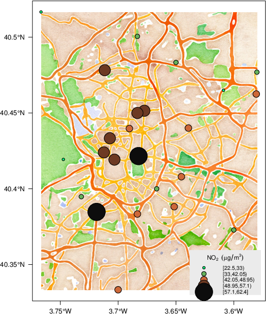