 ================================================
FILE: Demos/Data Analysis Workflow/report/report.html
================================================
================================================
FILE: Demos/Data Analysis Workflow/report/report.html
================================================
/report/report.Rmd.exploratory analysis
statistical analysis
predictive modeling
functional analysis
#set working directory
wd<-"C:/Users/Dmitry/Dropbox/Software/TeachingDemos/Demos/Data Analysis Workflow/"
setwd(wd)
#load dependancies
pkg<-c("ggplot2","dplyr","R.utils","fdrtool","caret","randomForest","pROC")
out<-lapply(pkg, function(x) {
if(!require(x,character.only = TRUE)) install.packages(x,character.only = TRUE)
}
)
#bioConductor
source("https://bioconductor.org/biocLite.R")
if(!require("pcaMethods")) biocLite("pcaMethods")
if(!require("pathview")) biocLite("pathview")
if(!require("KEGGREST")) biocLite("KEGGREST")
#load devium functions
#sourceDirectory( "R",recursive=TRUE)
source("http://pastebin.com/raw.php?i=UyDBTA57")#load data
setwd(wd)
load(file="data/data cube") # data.objtable(data.obj$raw$sample.meta$group)##
## healthy sick
## 27 27table(data.obj$raw$sample.meta$batch)##
## batch_1 batch_2
## 28 26data.cube<-data.obj$raw
args<-list( pca.data = data.cube$data,
pca.algorithm = "svd",
pca.components = 8,
pca.center = FALSE,
pca.scaling = "none",
pca.cv = "q2"
)
#calculate and view scree plot
res<-devium.pca.calculate(args,return="list",plot=TRUE)
#plot results
#scores highlighting healthy and sick
p.args<-list(
pca = res,
results = "scores",
color = data.cube$sample.meta[,"group",drop=FALSE],
font.size = 3
)
do.call("plot.PCA",p.args)
#loadings
p.args<-list(
pca = res,
results = "loadings",
color = data.cube$variable.meta[,"type",drop=FALSE],
font.size = 3
)
do.call("plot.PCA",p.args)
args<-list( pca.data = data.cube$data,
pca.algorithm = "svd",
pca.components = 8,
pca.center = TRUE,
pca.scaling = "uv",
pca.cv = "q2"
)
#calculate and view scree plot
res2<-devium.pca.calculate(args,return="list",plot=TRUE)
#loadings
p.args<-list(
pca = res2,
results = "loadings",
color = data.cube$variable.meta[,"type",drop=FALSE],
font.size = 3
)
do.call("plot.PCA",p.args)
#plot results
#scores highlighting healthy and sick
p.args<-list(
pca = res2,
results = "scores",
color = data.cube$sample.meta[,"group",drop=FALSE],
font.size = 3
)
do.call("plot.PCA",p.args)
p.args<-list(
pca = res2,
results = "scores",
color = data.cube$sample.meta[,"batch",drop=FALSE],
font.size =3
)
do.call("plot.PCA",p.args)
#get summaries and t-test stats
data.cube<-data.obj$normalized
data<-data.cube$data
meta<-data.cube$sample.meta[,"group",drop=FALSE]
#get summary
.summary<-stats.summary(data,comp.obj=meta,formula=colnames(meta),sigfigs=3,log=FALSE,rel=1,do.stats=TRUE)## Generating data summary...
## Conducting tests...
## Conducting FDR corrections...stats.obj<-cbind(data.cube$variable.meta,.summary)
stats.obj %>% arrange(group_p.values) %>% head(.)## ID description type
## 1 C00077 ornithine metabolite
## 2 C02477 tocopherol alpha metabolite
## 3 C00097 cysteine metabolite
## 4 C00031 glucose metabolite
## 5 C00170 5'-deoxy-5'-methylthioadenosine metabolite
## 6 C00385 xanthine metabolite
## healthy.mean.....std.dev sick.mean.....std.dev mean.sick_mean.healthy
## 1 7300 +/- 2900 3910 +/- 2100 0.54
## 2 1160 +/- 1400 2600 +/- 1200 2.24
## 3 5160 +/- 2500 8460 +/- 3400 1.64
## 4 335000 +/- 2e+05 144000 +/- 140000 0.43
## 5 216 +/- 83 355 +/- 160 1.64
## 6 574 +/- 350 1670 +/- 1500 2.91
## group_p.values group_adjusted.p.values group_q.values
## 1 9.433317e-06 0.001886663 0.000900412
## 2 1.505034e-04 0.007714558 0.003632462
## 3 1.507843e-04 0.007714558 0.003633836
## 4 1.542912e-04 0.007714558 0.003650646
## 5 2.004055e-04 0.008016221 0.003825749
## 6 3.909048e-04 0.013030159 0.006072846#write.csv(stats.obj,file="results/statistical_results.csv")top.met<-stats.obj %>% filter(type =="metabolite") %>%
arrange(group_p.values) %>% dplyr::select(ID) %>%
dplyr:: slice(.,1) %>% unlist(.) %>% as.character(.)
id<-as.character(stats.obj$ID) %in% top.met
tmp.data<-data.frame(data[,id,drop=FALSE],meta)
#make plot
ggplot(tmp.data,aes_string(x="group",y=colnames(tmp.data)[1],fill="group")) +
geom_boxplot() + ggtitle(as.character(stats.obj$description[id])) +ylab("")
top.met<-stats.obj %>% filter(type =="protein") %>%
arrange(group_p.values) %>% dplyr::select(ID) %>%
dplyr:: slice(.,1) %>% unlist(.) %>% as.character(.)
id<-as.character(stats.obj$ID) %in% top.met
tmp.data<-data.frame(data[,id,drop=FALSE],meta)
#make plot
ggplot(tmp.data,aes_string(x="group",y=colnames(tmp.data)[1],fill="group")) +
geom_boxplot() + ggtitle(as.character(stats.obj$description[id])) +ylab("")
mtry parameter is optimized to maximize the are under the reciever operator characteristic curve (AUCROC).#create a classification model using random forests
#generate training/test set
set.seed(998)
data<-data.cube$data
inTraining <- createDataPartition(data.cube$sample.meta$group, p = 2/3, list = FALSE)
train.data <- data[ inTraining,]
test.data <- data[-inTraining,]
train.y <- data.cube$sample.meta$group[ inTraining] %>% droplevels()
test.y <- data.cube$sample.meta$group[ -inTraining] %>% droplevels()
#set model parameters
fitControl <- trainControl(## 10-fold CV
method = "repeatedcv",
number = 3,
## repeated ten times
repeats = 3,
classProbs = TRUE,
summaryFunction = twoClassSummary
)
#fit model to the training data
set.seed(825)
fit<- train(train.y ~ ., data = train.data,
method = "rf",
trControl = fitControl,
metric = "ROC",
tuneLength = 3
)mtry or the number of variables randomly sampled as candidates at each split.fit## Random Forest
##
## 36 samples
## 199 predictors
## 2 classes: 'healthy', 'sick'
##
## No pre-processing
## Resampling: Cross-Validated (3 fold, repeated 3 times)
##
## Summary of sample sizes: 24, 24, 24, 24, 24, 24, ...
##
## Resampling results across tuning parameters:
##
## mtry ROC Sens Spec ROC SD Sens SD Spec SD
## 2 0.7870370 0.7222222 0.7777778 0.08098544 0.2041241 0.1666667
## 101 0.8549383 0.7777778 0.7592593 0.10090044 0.1443376 0.2060055
## 200 0.8750000 0.8333333 0.7222222 0.09107554 0.1178511 0.2204793
##
## ROC was used to select the optimal model using the largest value.
## The final value used for the model was mtry = 200.#predict the test set
pred<-predict(fit,newdata=test.data)
prob<-predict(fit,newdata=test.data,type="prob")
obs<-test.y
table(pred,obs)## obs
## pred healthy sick
## healthy 7 2
## sick 2 7#get performance stats
twoClassSummary(data=data.frame(obs,pred,prob),lev=levels(pred))## ROC Sens Spec
## 0.9135802 0.7777778 0.7777778x<-roc(obs,prob[,levels(pred)[1]],silent = TRUE)
plot(x)
##
## Call:
## roc.default(response = obs, predictor = prob[, levels(pred)[1]], silent = TRUE)
##
## Data: prob[, levels(pred)[1]] in 9 controls (obs healthy) > 9 cases (obs sick).
## Area under the curve: 0.9136#need to get variable names
vip<-varImp(fit)$importance # need to keep rownames
vip<-vip[order(vip[,1],decreasing=TRUE),,drop=FALSE][1:10,,drop=FALSE]
id<-colnames(train.data) %in% gsub('`','',rownames(vip))
tmp.data<-data.frame(importance=vip[,1],variable=factor(stats.obj$description[id],levels=stats.obj$description[id],ordered=FALSE))
#plot
ggplot(tmp.data, aes(x=variable,y=importance)) + geom_bar(stat="identity") + coord_flip()
id<-as.character(stats.obj$description) %in% as.character(tmp.data[1,2])
tmp.data<-data.frame(data[,id,drop=FALSE],meta)
#make plot
ggplot(tmp.data,aes_string(x="group",y=colnames(tmp.data)[1],fill="group")) +
geom_boxplot() + ggtitle(as.character(stats.obj$description[id])) +ylab("")
results/statistical_results_sig.csv). We can view the full analysis results in results/IMPaLA_results.csv. next lets take an enriched pathway and fisualize the fold changes between sick and healthy in the enriched species.#format data to show fold changes in pathway
#get formatted data for pathview
library(KEGGREST)
library(pathview)
data<-stats.obj
#metabolite
met<-data %>% dplyr::filter(type =="metabolite") %>%
dplyr::select(ID,mean.sick_mean.healthy) %>%
mutate(FC=log(mean.sick_mean.healthy)) %>% dplyr::select(-mean.sick_mean.healthy)
#protein
prot<-data %>% dplyr::filter(type =="protein") %>%
dplyr::select(ID,mean.sick_mean.healthy) %>%
mutate(FC=log(mean.sick_mean.healthy)) %>% dplyr::select(-mean.sick_mean.healthy)
#set rownames
rownames(met)<-met[,1];met<-met[,-1,drop=FALSE]
rownames(prot)<-prot[,1];prot<-prot[,-1,drop=FALSE]
#select pathway to view
path<-"Glycolysis / Gluconeogenesis"head(met)## FC
## C00379 0.41871033
## C00385 1.06815308
## C00105 0.07696104
## C00299 -0.24846136
## C00366 0.33647224
## C00086 -0.05129329head(prot)## FC
## SPTAN1 -0.3424903
## CFH 0.1133287
## VPS13C 0.3148107
## XRCC6 1.0715836
## APOA1 -0.1392621
## SUPT16H 0.7129498data(korg)
organism <- "homo sapiens"
matches <- unlist(sapply(1:ncol(korg), function(i) {
agrep(organism, korg[, i])
}))
(kegg.code <- korg[matches, 1, drop = F])## kegg.code
## [1,] "hsa"setwd(wd)
pathways <- keggList("pathway", kegg.code)
#get code of our pathway of interest
map<-grepl(path,pathways) %>% pathways[.] %>% names(.) %>% gsub("path:","",.)
map## [1] "hsa00010"#create image
setwd("report")
pv.out <- pathview(gene.data = prot, cpd.data = met, gene.idtype = "SYMBOL",
pathway.id = map, species = kegg.code, out.suffix = map, keys.align = "y",
kegg.native = T, match.data = T, key.pos = "topright")
© Dmitry Grapov (2015) 
 ##### The following is an example of a data analysis strategy for an integrated metabolomic and proteomic data set. This tutorial is meant to give examples of some of the major common steps in an omic integration analysis workflow. You can check out all of the code in `/report/report.Rmd`.
1. exploratory analysis
2. statistical analysis
3. predictive modeling
4. functional analysis
```r
#set working directory
wd<-"C:/Users/Dmitry/Dropbox/Software/TeachingDemos/Demos/Data Analysis Workflow/"
setwd(wd)
#load dependancies
pkg<-c("ggplot2","dplyr","R.utils","fdrtool","caret","randomForest","pROC")
out<-lapply(pkg, function(x) {
if(!require(x,character.only = TRUE)) install.packages(x,character.only = TRUE)
}
)
#bioConductor
source("https://bioconductor.org/biocLite.R")
if(!require("pcaMethods")) biocLite("pcaMethods")
if(!require("pathview")) biocLite("pathview")
if(!require("KEGGREST")) biocLite("KEGGREST")
#load devium functions
#sourceDirectory( "R",recursive=TRUE)
source("http://pastebin.com/raw.php?i=UyDBTA57")
```
```r
#load data
setwd(wd)
load(file="data/data cube") # data.obj
```
##### This data set contains 200 measurements for 54 samples. The samples are comprised of sick and healthy patients measured across two analytical batches.
```r
table(data.obj$raw$sample.meta$group)
```
```
##
## healthy sick
## 27 27
```
```r
table(data.obj$raw$sample.meta$batch)
```
```
##
## batch_1 batch_2
## 28 26
```
****
### Exploratory Analysis
****
##### A critical aspect of any data analysis should be to carry out an exploratory data analysis to see if there are any strange trends. Below is an example of a Principal Components Analysis (PCA). Lets start by looking at the raw data and caclculate PCA with out anys scaling.
##### PCA has three main components we can use to evaluate our data.
##### 1. Variance explained by each component
```r
data.cube<-data.obj$raw
args<-list( pca.data = data.cube$data,
pca.algorithm = "svd",
pca.components = 8,
pca.center = FALSE,
pca.scaling = "none",
pca.cv = "q2"
)
#calculate and view scree plot
res<-devium.pca.calculate(args,return="list",plot=TRUE)
```

##### The scree plot above shows the total variance in the data explained (top) and the cumulative varince explained (bottom) by each principal component (PC). The green bars in the bottom plot show the cross-validated variance explained which can be used to give us an idea bout the stability of calculated components. How many PCs to keep can be determined based on a few criteria 1) each PC should explain some minnimum variance and 2) calculate enough PCS to explain some target variance. The hashed line in the top plot shows PCs which explain less than 1% variance and the hashed line in the bottom plot shows how many PCs arerequired to explain 80% of the varince in the data. Based on an evaluation of the scree plot we may select 2 or 3 PCs. The cross-validated varince explained (green bars) also suggest that the variance explained does not increase after the first 2 PCs.
##### 2. The sample scores can be used to visualize multivariete similarities in samples given all the varibles for each PC. Lets plot the scores and highlight the sick and healthy groups.
```r
#plot results
#scores highlighting healthy and sick
p.args<-list(
pca = res,
results = "scores",
color = data.cube$sample.meta[,"group",drop=FALSE],
font.size = 3
)
do.call("plot.PCA",p.args)
```

#### Based on the scores above the sick and healthy samples look fairly similiar. Lets next look at the variable loadings.
#### 3. Variable loadings show the contribution of each varible to the calculated scores.
```r
#loadings
p.args<-list(
pca = res,
results = "loadings",
color = data.cube$variable.meta[,"type",drop=FALSE],
font.size = 3
)
do.call("plot.PCA",p.args)
```

#### Evaluation of the loadings suggest that variance variables X838 abd X454 explain ~90% of the varince in the data. Because we did not scale the data before conducting PCA, variables with the largest magnitude will contribute most to varince explained.
#### Next lets recalculate the PCA and mean center and scale all the variables by their standard deviation (autoscale).
#### Variance explained
```r
args<-list( pca.data = data.cube$data,
pca.algorithm = "svd",
pca.components = 8,
pca.center = TRUE,
pca.scaling = "uv",
pca.cv = "q2"
)
#calculate and view scree plot
res2<-devium.pca.calculate(args,return="list",plot=TRUE)
```

#### Variable loadings
```r
#loadings
p.args<-list(
pca = res2,
results = "loadings",
color = data.cube$variable.meta[,"type",drop=FALSE],
font.size = 3
)
do.call("plot.PCA",p.args)
```

#### Sample scores
```r
#plot results
#scores highlighting healthy and sick
p.args<-list(
pca = res2,
results = "scores",
color = data.cube$sample.meta[,"group",drop=FALSE],
font.size = 3
)
do.call("plot.PCA",p.args)
```

#### There are some noticible differences in PCA after we scaled our data.
1. Variable magnitude no longer drives the majority of the variance.
2. We can see more resolution in variable loadings for the first 2 PCs.
3. There is an unexplained group structure in the score.
#### Next we can try mapping other meta data to score to see if we can explain the cluster pattern. Lets show the analytical batches in the samples scores.
```r
p.args<-list(
pca = res2,
results = "scores",
color = data.cube$sample.meta[,"batch",drop=FALSE],
font.size =3
)
do.call("plot.PCA",p.args)
```

#### We can see in the scores above that the analytical batch nicely explains 35% of the varince in the data. This is a common problem in large data sets which is best handled using various data normalization methods. Here is some more information about implementing data normalizations.
###### [Metabolomics and Beyond: Challenges and Strategies for Next-generation Omic Analyses](https://imdevsoftware.files.wordpress.com/2015/09/clipboard01.png?w=300&h=225)
[](https://www.youtube.com/watch?v=4AhBN5Q1oMs)
##### [Evaluation of data normalization methods](http://www.slideshare.net/dgrapov/case-study-metabolomic-data-normalization-example)
****
#### [Part 3](http://www.slideshare.net/dgrapov/data-analysis-workflows-part-2-2015?related=1)
##### The following is an example of a data analysis strategy for an integrated metabolomic and proteomic data set. This tutorial is meant to give examples of some of the major common steps in an omic integration analysis workflow. You can check out all of the code in `/report/report.Rmd`.
1. exploratory analysis
2. statistical analysis
3. predictive modeling
4. functional analysis
```r
#set working directory
wd<-"C:/Users/Dmitry/Dropbox/Software/TeachingDemos/Demos/Data Analysis Workflow/"
setwd(wd)
#load dependancies
pkg<-c("ggplot2","dplyr","R.utils","fdrtool","caret","randomForest","pROC")
out<-lapply(pkg, function(x) {
if(!require(x,character.only = TRUE)) install.packages(x,character.only = TRUE)
}
)
#bioConductor
source("https://bioconductor.org/biocLite.R")
if(!require("pcaMethods")) biocLite("pcaMethods")
if(!require("pathview")) biocLite("pathview")
if(!require("KEGGREST")) biocLite("KEGGREST")
#load devium functions
#sourceDirectory( "R",recursive=TRUE)
source("http://pastebin.com/raw.php?i=UyDBTA57")
```
```r
#load data
setwd(wd)
load(file="data/data cube") # data.obj
```
##### This data set contains 200 measurements for 54 samples. The samples are comprised of sick and healthy patients measured across two analytical batches.
```r
table(data.obj$raw$sample.meta$group)
```
```
##
## healthy sick
## 27 27
```
```r
table(data.obj$raw$sample.meta$batch)
```
```
##
## batch_1 batch_2
## 28 26
```
****
### Exploratory Analysis
****
##### A critical aspect of any data analysis should be to carry out an exploratory data analysis to see if there are any strange trends. Below is an example of a Principal Components Analysis (PCA). Lets start by looking at the raw data and caclculate PCA with out anys scaling.
##### PCA has three main components we can use to evaluate our data.
##### 1. Variance explained by each component
```r
data.cube<-data.obj$raw
args<-list( pca.data = data.cube$data,
pca.algorithm = "svd",
pca.components = 8,
pca.center = FALSE,
pca.scaling = "none",
pca.cv = "q2"
)
#calculate and view scree plot
res<-devium.pca.calculate(args,return="list",plot=TRUE)
```

##### The scree plot above shows the total variance in the data explained (top) and the cumulative varince explained (bottom) by each principal component (PC). The green bars in the bottom plot show the cross-validated variance explained which can be used to give us an idea bout the stability of calculated components. How many PCs to keep can be determined based on a few criteria 1) each PC should explain some minnimum variance and 2) calculate enough PCS to explain some target variance. The hashed line in the top plot shows PCs which explain less than 1% variance and the hashed line in the bottom plot shows how many PCs arerequired to explain 80% of the varince in the data. Based on an evaluation of the scree plot we may select 2 or 3 PCs. The cross-validated varince explained (green bars) also suggest that the variance explained does not increase after the first 2 PCs.
##### 2. The sample scores can be used to visualize multivariete similarities in samples given all the varibles for each PC. Lets plot the scores and highlight the sick and healthy groups.
```r
#plot results
#scores highlighting healthy and sick
p.args<-list(
pca = res,
results = "scores",
color = data.cube$sample.meta[,"group",drop=FALSE],
font.size = 3
)
do.call("plot.PCA",p.args)
```

#### Based on the scores above the sick and healthy samples look fairly similiar. Lets next look at the variable loadings.
#### 3. Variable loadings show the contribution of each varible to the calculated scores.
```r
#loadings
p.args<-list(
pca = res,
results = "loadings",
color = data.cube$variable.meta[,"type",drop=FALSE],
font.size = 3
)
do.call("plot.PCA",p.args)
```

#### Evaluation of the loadings suggest that variance variables X838 abd X454 explain ~90% of the varince in the data. Because we did not scale the data before conducting PCA, variables with the largest magnitude will contribute most to varince explained.
#### Next lets recalculate the PCA and mean center and scale all the variables by their standard deviation (autoscale).
#### Variance explained
```r
args<-list( pca.data = data.cube$data,
pca.algorithm = "svd",
pca.components = 8,
pca.center = TRUE,
pca.scaling = "uv",
pca.cv = "q2"
)
#calculate and view scree plot
res2<-devium.pca.calculate(args,return="list",plot=TRUE)
```

#### Variable loadings
```r
#loadings
p.args<-list(
pca = res2,
results = "loadings",
color = data.cube$variable.meta[,"type",drop=FALSE],
font.size = 3
)
do.call("plot.PCA",p.args)
```

#### Sample scores
```r
#plot results
#scores highlighting healthy and sick
p.args<-list(
pca = res2,
results = "scores",
color = data.cube$sample.meta[,"group",drop=FALSE],
font.size = 3
)
do.call("plot.PCA",p.args)
```

#### There are some noticible differences in PCA after we scaled our data.
1. Variable magnitude no longer drives the majority of the variance.
2. We can see more resolution in variable loadings for the first 2 PCs.
3. There is an unexplained group structure in the score.
#### Next we can try mapping other meta data to score to see if we can explain the cluster pattern. Lets show the analytical batches in the samples scores.
```r
p.args<-list(
pca = res2,
results = "scores",
color = data.cube$sample.meta[,"batch",drop=FALSE],
font.size =3
)
do.call("plot.PCA",p.args)
```

#### We can see in the scores above that the analytical batch nicely explains 35% of the varince in the data. This is a common problem in large data sets which is best handled using various data normalization methods. Here is some more information about implementing data normalizations.
###### [Metabolomics and Beyond: Challenges and Strategies for Next-generation Omic Analyses](https://imdevsoftware.files.wordpress.com/2015/09/clipboard01.png?w=300&h=225)
[](https://www.youtube.com/watch?v=4AhBN5Q1oMs)
##### [Evaluation of data normalization methods](http://www.slideshare.net/dgrapov/case-study-metabolomic-data-normalization-example)
****
#### [Part 3](http://www.slideshare.net/dgrapov/data-analysis-workflows-part-2-2015?related=1)
 ### Statistical Analysis
****
##### Next lets carry out a statistical analysis and summarise the changes between the sick and ghealthy groups. Below we identify significantly altered analytes using a basic t-test with adjustment for multiple hypotheses tested. We probably want to use more sophisticated and non-parametric tests for real applications.
```r
#get summaries and t-test stats
data.cube<-data.obj$normalized
data<-data.cube$data
meta<-data.cube$sample.meta[,"group",drop=FALSE]
#get summary
.summary<-stats.summary(data,comp.obj=meta,formula=colnames(meta),sigfigs=3,log=FALSE,rel=1,do.stats=TRUE)
```
```
## Generating data summary...
## Conducting tests...
## Conducting FDR corrections...
```
```r
stats.obj<-cbind(data.cube$variable.meta,.summary)
stats.obj %>% arrange(group_p.values) %>% head(.)
```
```
## ID description type
## 1 C00077 ornithine metabolite
## 2 C02477 tocopherol alpha metabolite
## 3 C00097 cysteine metabolite
## 4 C00031 glucose metabolite
## 5 C00170 5'-deoxy-5'-methylthioadenosine metabolite
## 6 C00385 xanthine metabolite
## healthy.mean.....std.dev sick.mean.....std.dev mean.sick_mean.healthy
## 1 7300 +/- 2900 3910 +/- 2100 0.54
## 2 1160 +/- 1400 2600 +/- 1200 2.24
## 3 5160 +/- 2500 8460 +/- 3400 1.64
## 4 335000 +/- 2e+05 144000 +/- 140000 0.43
## 5 216 +/- 83 355 +/- 160 1.64
## 6 574 +/- 350 1670 +/- 1500 2.91
## group_p.values group_adjusted.p.values group_q.values
## 1 9.433317e-06 0.001886663 0.000900412
## 2 1.505034e-04 0.007714558 0.003632462
## 3 1.507843e-04 0.007714558 0.003633836
## 4 1.542912e-04 0.007714558 0.003650646
## 5 2.004055e-04 0.008016221 0.003825749
## 6 3.909048e-04 0.013030159 0.006072846
```
```r
#write.csv(stats.obj,file="results/statistical_results.csv")
```
#### We can visualize the differences in means for the top most altered metabolite and protein as a box plot.
```r
top.met<-stats.obj %>% filter(type =="metabolite") %>%
arrange(group_p.values) %>% dplyr::select(ID) %>%
dplyr:: slice(.,1) %>% unlist(.) %>% as.character(.)
id<-as.character(stats.obj$ID) %in% top.met
tmp.data<-data.frame(data[,id,drop=FALSE],meta)
#make plot
ggplot(tmp.data,aes_string(x="group",y=colnames(tmp.data)[1],fill="group")) +
geom_boxplot() + ggtitle(as.character(stats.obj$description[id])) +ylab("")
```

```r
top.met<-stats.obj %>% filter(type =="protein") %>%
arrange(group_p.values) %>% dplyr::select(ID) %>%
dplyr:: slice(.,1) %>% unlist(.) %>% as.character(.)
id<-as.character(stats.obj$ID) %in% top.met
tmp.data<-data.frame(data[,id,drop=FALSE],meta)
#make plot
ggplot(tmp.data,aes_string(x="group",y=colnames(tmp.data)[1],fill="group")) +
geom_boxplot() + ggtitle(as.character(stats.obj$description[id])) +ylab("")
```

****
### Predictive Modeling
****
#### Next we can try a generate a non-linear multivarite classification model to identify important variables in our data. Below we will train and validate a random forest classifier. The full data set is split into 2/3 trainning and 1/3 test set while keeping the propotion of sick and healthy samples equivalent. The model is trained using 3-fold cross-validation repeated 3 times and the ```mtry``` parameter is optimized to maximize the are under the reciever operator characteristic curve (AUCROC).
```r
#create a classification model using random forests
#generate training/test set
set.seed(998)
data<-data.cube$data
inTraining <- createDataPartition(data.cube$sample.meta$group, p = 2/3, list = FALSE)
train.data <- data[ inTraining,]
test.data <- data[-inTraining,]
train.y <- data.cube$sample.meta$group[ inTraining] %>% droplevels()
test.y <- data.cube$sample.meta$group[ -inTraining] %>% droplevels()
#set model parameters
fitControl <- trainControl(## 10-fold CV
method = "repeatedcv",
number = 3,
## repeated ten times
repeats = 3,
classProbs = TRUE,
summaryFunction = twoClassSummary
)
#fit model to the training data
set.seed(825)
fit<- train(train.y ~ ., data = train.data,
method = "rf",
trControl = fitControl,
metric = "ROC",
tuneLength = 3
)
```
#### Below the optimal model is chosen while varying the ```mtry``` or the number of variables randomly sampled as candidates at each split.
```r
fit
```
```
## Random Forest
##
## 36 samples
## 199 predictors
## 2 classes: 'healthy', 'sick'
##
## No pre-processing
## Resampling: Cross-Validated (3 fold, repeated 3 times)
##
## Summary of sample sizes: 24, 24, 24, 24, 24, 24, ...
##
## Resampling results across tuning parameters:
##
## mtry ROC Sens Spec ROC SD Sens SD Spec SD
## 2 0.7870370 0.7222222 0.7777778 0.08098544 0.2041241 0.1666667
## 101 0.8549383 0.7777778 0.7592593 0.10090044 0.1443376 0.2060055
## 200 0.8750000 0.8333333 0.7222222 0.09107554 0.1178511 0.2204793
##
## ROC was used to select the optimal model using the largest value.
## The final value used for the model was mtry = 200.
```
#### Next we can evaluate the model performance based on predictions for the test set. We can also look at the ROC curve.
```r
#predict the test set
pred<-predict(fit,newdata=test.data)
prob<-predict(fit,newdata=test.data,type="prob")
obs<-test.y
table(pred,obs)
```
```
## obs
## pred healthy sick
## healthy 7 2
## sick 2 7
```
```r
#get performance stats
twoClassSummary(data=data.frame(obs,pred,prob),lev=levels(pred))
```
```
## ROC Sens Spec
## 0.9135802 0.7777778 0.7777778
```
#### We can also look at the ROC curve.
```r
x<-roc(obs,prob[,levels(pred)[1]],silent = TRUE)
plot(x)
```

```
##
## Call:
## roc.default(response = obs, predictor = prob[, levels(pred)[1]], silent = TRUE)
##
## Data: prob[, levels(pred)[1]] in 9 controls (obs healthy) > 9 cases (obs sick).
## Area under the curve: 0.9136
```
#### Having validated our model next we can look at the most important variables driving the classification. We can look at the differences in performance when each variable is randomly permuted or the VIP.
```r
#need to get variable names
vip<-varImp(fit)$importance # need to keep rownames
vip<-vip[order(vip[,1],decreasing=TRUE),,drop=FALSE][1:10,,drop=FALSE]
id<-colnames(train.data) %in% gsub('`','',rownames(vip))
tmp.data<-data.frame(importance=vip[,1],variable=factor(stats.obj$description[id],levels=stats.obj$description[id],ordered=FALSE))
#plot
ggplot(tmp.data, aes(x=variable,y=importance)) + geom_bar(stat="identity") + coord_flip()
```

```r
id<-as.character(stats.obj$description) %in% as.character(tmp.data[1,2])
tmp.data<-data.frame(data[,id,drop=FALSE],meta)
#make plot
ggplot(tmp.data,aes_string(x="group",y=colnames(tmp.data)[1],fill="group")) +
geom_boxplot() + ggtitle(as.character(stats.obj$description[id])) +ylab("")
```

****
### Functional Analysis
****
#### Finally we can identify enriched biological pathways based on the integrated changes in genes and proteins. [IMPaLA: Integrated Molecular Pathway Level Analysis](http://impala.molgen.mpg.de/) can be used to calculate enriched pathways in genes or proteins and metabolites.To do this we can querry the significantly alterd proteins and metabolites for enriched pathways (see `results/statistical_results_sig.csv`). We can view the full analysis results in `results/IMPaLA_results.csv`. next lets take an enriched pathway and fisualize the fold changes between sick and healthy in the enriched species.
```r
#format data to show fold changes in pathway
#get formatted data for pathview
library(KEGGREST)
library(pathview)
data<-stats.obj
#metabolite
met<-data %>% dplyr::filter(type =="metabolite") %>%
dplyr::select(ID,mean.sick_mean.healthy) %>%
mutate(FC=log(mean.sick_mean.healthy)) %>% dplyr::select(-mean.sick_mean.healthy)
#protein
prot<-data %>% dplyr::filter(type =="protein") %>%
dplyr::select(ID,mean.sick_mean.healthy) %>%
mutate(FC=log(mean.sick_mean.healthy)) %>% dplyr::select(-mean.sick_mean.healthy)
#set rownames
rownames(met)<-met[,1];met<-met[,-1,drop=FALSE]
rownames(prot)<-prot[,1];prot<-prot[,-1,drop=FALSE]
#select pathway to view
path<-"Glycolysis / Gluconeogenesis"
```
#### Lets take a looka at the Glycolysis / Gluconeogenesis pathway. Our data needs to be formatted as below. You can also take a look at the following more detailed example of [mapping fold changes to biochemical pathways](https://github.com/dgrapov/TeachingDemos/blob/master/Demos/Pathway%20Analysis/KEGG%20Pathway%20Enrichment.md).
#### Metabolite data showing KEGG ids and log fold change
```r
head(met)
```
```
## FC
## C00379 0.41871033
## C00385 1.06815308
## C00105 0.07696104
## C00299 -0.24846136
## C00366 0.33647224
## C00086 -0.05129329
```
#### Protein data showing the Entrez gene name and log fold changes
```r
head(prot)
```
```
## FC
## SPTAN1 -0.3424903
## CFH 0.1133287
## VPS13C 0.3148107
## XRCC6 1.0715836
## APOA1 -0.1392621
## SUPT16H 0.7129498
```
#### Next we need to get the pathway code for or pathway of interest.
```r
data(korg)
organism <- "homo sapiens"
matches <- unlist(sapply(1:ncol(korg), function(i) {
agrep(organism, korg[, i])
}))
(kegg.code <- korg[matches, 1, drop = F])
```
```
## kegg.code
## [1,] "hsa"
```
#### Now we can visualize the changes between sick and healthy in the Glycolysis / Gluconeogenesis pathway.
```r
setwd(wd)
pathways <- keggList("pathway", kegg.code)
#get code of our pathway of interest
map<-grepl(path,pathways) %>% pathways[.] %>% names(.) %>% gsub("path:","",.)
map
```
```
## [1] "hsa00010"
```
```r
#create image
setwd("report")
pv.out <- pathview(gene.data = prot, cpd.data = met, gene.idtype = "SYMBOL",
pathway.id = map, species = kegg.code, out.suffix = map, keys.align = "y",
kegg.native = T, match.data = T, key.pos = "topright")
```

****
#### This concludes this short tutorial. You may also find the following links useful.
* [Software tools](https://github.com/dgrapov)
* [More examples and demos](https://imdevsoftware.wordpress.com/)
© Dmitry Grapov (2015)
================================================
FILE: Demos/Data Analysis Workflow/results/IMPaLA_results.csv
================================================
pathway_name,pathway_source,num_overlapping_genes,overlapping_genes,num_all_pathway_genes,P_genes,Q_genes,num_overlapping_metabolites,overlapping_metabolites,num_all_pathway_metabolites,P_metabolites,Q_metabolites,P_joint,Q_joint
Metabolism,Reactome,3,GLS;IVD;ACSS2,1427 (1485),0.505,1,26,C00077;C00158;C00116;C00366;C00385;C00170;C01835;C00245;C00836;C00180;C00315;C00041;C00047;C00106;C00148;C00791;C00020;C00025;C00197;C00097;C00327;C00130;C00135;C03546;C00989;C00346,808 (1017),3.54E-13,8.03E-10,5.43E-12,5.61E-09
Transmembrane transport of small molecules,Reactome,0,,594 (623),1,1,16,C00077;C00106;C00116;C00148;C00245;C00158;C00791;C00020;C00025;C00097;C01571;C00366;C00315;C00041;C00047;C00135,204 (216),4.50E-13,8.03E-10,1.32E-11,6.85E-09
Metabolism of amino acids and derivatives,Reactome,2,IVD;GLS,145 (152),0.0292,1,14,C00077;C00148;C00245;C00791;C00020;C00197;C00025;C00170;C00097;C00315;C00327;C00041;C00047;C00135,181 (190),2.62E-11,1.87E-08,2.21E-11,7.61E-09
Metabolism of amino acids and derivatives,Wikipathways,0,,0 (0),1,1,14,C00077;C00148;C00245;C00791;C00020;C00197;C00025;C00170;C00097;C00315;C00327;C00041;C00047;C00135,174 (187),1.52E-11,1.36E-08,1.52E-11,1.36E-08
SLC-mediated transmembrane transport,Reactome,0,,261 (265),1,1,14,C00077;C00106;C00148;C00135;C00245;C00158;C00791;C00025;C00097;C01571;C00315;C00041;C00047;C00366,160 (165),4.77E-12,5.68E-09,1.29E-10,3.34E-08
Central carbon metabolism in cancer - Homo sapiens (human),KEGG,1,GLS,66 (67),0.116,1,8,C00158;C00148;C00031;C00197;C00025;C00097;C00041;C00135,37 (37),2.36E-10,9.37E-08,6.92E-10,1.43E-07
ABC transporters - Homo sapiens (human),KEGG,0,,44 (44),1,1,12,C00077;C00116;C00148;C00245;C00379;C00031;C00025;C00047;C00315;C00041;C01835;C00135,123 (123),6.60E-11,3.37E-08,1.61E-09,2.39E-07
Amino acid transport across the plasma membrane,Reactome,0,,31 (31),1,1,8,C00077;C00148;C00245;C00025;C00097;C00041;C00047;C00135,32 (32),6.61E-11,3.37E-08,1.62E-09,2.39E-07
Transport of glucose and other sugars_ bile salts and organic acids_ metal ions and amine compounds,Reactome,0,,98 (101),1,1,10,C00158;C00148;C00366;C00791;C00245;C00097;C00315;C00041;C00047;C00135,78 (83),2.28E-10,9.37E-08,5.30E-09,6.86E-07
Urea cycle and metabolism of arginine_ proline_ glutamate_ aspartate and asparagine,EHMN,1,GLS,105 (107),0.178,1,11,C00077;C00148;C00020;C00025;C00170;C00097;C00315;C00327;C00041;C00047;C00989,125 (125),1.52E-09,4.53E-07,6.24E-09,7.18E-07
tRNA charging,HumanCyc,0,,41 (44),1,1,7,C00148;C00020;C00025;C00097;C00041;C00047;C00135,24 (24),3.55E-10,1.27E-07,8.07E-09,7.78E-07
Class I MHC mediated antigen processing & presentation,Reactome,2,SEC24C;SEC13,208 (224),0.0561,1,7,C00148;C00020;C00025;C00097;C00041;C00047;C00135,35 (35),6.48E-09,1.54E-06,8.27E-09,7.78E-07
Glucose Homeostasis,Wikipathways,0,,0 (0),1,1,6,C00077;C00116;C00031;C00327;C00047;C00135,21 (21),8.50E-09,1.78E-06,8.50E-09,1.78E-06
Amino acid and oligopeptide SLC transporters,Reactome,0,,49 (49),1,1,8,C00077;C00148;C00245;C00025;C00097;C00041;C00047;C00135,45 (45),1.26E-09,4.10E-07,2.71E-08,2.34E-06
Transport of inorganic cations/anions and amino acids/oligopeptides,Reactome,0,,94 (95),1,1,8,C00077;C00148;C00245;C00025;C00097;C00041;C00047;C00135,48 (48),2.17E-09,5.97E-07,4.55E-08,3.63E-06
Amino acid synthesis and interconversion (transamination),Reactome,1,GLS,17 (17),0.0311,1,6,C00077;C00148;C00020;C00197;C00025;C00041,32 (32),1.33E-07,1.83E-05,8.42E-08,6.22E-06
Adaptive Immune System,Reactome,3,SEC24C;EVL;SEC13,558 (608),0.0819,1,7,C00148;C00020;C00025;C00097;C00041;C00047;C00135,48 (48),6.59E-08,1.21E-05,1.08E-07,7.46E-06
Endosomal/Vacuolar pathway,Reactome,0,,12 (12),1,1,6,C00148;C00025;C00097;C00041;C00047;C00135,20 (20),6.10E-09,1.54E-06,1.22E-07,7.86E-06
Proton/oligonucleotide cotransporters,Reactome,0,,4 (4),1,1,6,C00148;C00025;C00097;C00041;C00047;C00135,21 (21),8.50E-09,1.78E-06,1.66E-07,1.01E-05
Transport of inorganic cations-anions and amino acids-oligopeptides,Wikipathways,0,,0 (0),1,1,6,C00148;C00025;C00097;C00041;C00047;C00135,31 (32),1.09E-07,1.56E-05,1.09E-07,1.56E-05
γ-glutamyl cycle,HumanCyc,0,,11 (12),1,1,7,C00077;C00148;C00025;C00097;C00041;C00047;C00135,43 (47),2.97E-08,5.89E-06,5.44E-07,3.13E-05
Antigen processing-Cross presentation,Reactome,0,,32 (32),1,1,6,C00148;C00025;C00097;C00041;C00047;C00135,29 (29),7.11E-08,1.21E-05,1.24E-06,6.42E-05
leukotriene biosynthesis,HumanCyc,0,,6 (7),1,1,6,C00148;C00025;C00097;C00041;C00047;C00135,29 (30),7.11E-08,1.21E-05,1.24E-06,6.42E-05
tRNA Aminoacylation,Wikipathways,0,,0 (0),1,1,7,C00148;C00020;C00025;C00097;C00041;C00047;C00135,65 (65),5.67E-07,6.53E-05,5.67E-07,6.53E-05
Glutathione synthesis and recycling,Reactome,0,,14 (17),1,1,6,C00148;C00025;C00097;C00041;C00047;C00135,30 (31),8.83E-08,1.37E-05,1.52E-06,7.16E-05
Urea cycle and metabolism of amino groups,Wikipathways,0,,20 (20),1,1,6,C00077;C00148;C00791;C00025;C00315;C00327,30 (30),8.83E-08,1.37E-05,1.52E-06,7.16E-05
Na+/Cl- dependent neurotransmitter transporters,Reactome,0,,19 (19),1,1,6,C00148;C00245;C00097;C00041;C00047;C00135,31 (31),1.09E-07,1.56E-05,1.85E-06,8.35E-05
Phase II conjugation,Wikipathways,0,,0 (0),1,1,8,C00148;C00020;C00025;C00097;C00180;C00041;C00047;C00135,102 (115),9.38E-07,9.57E-05,9.38E-07,9.57E-05
Nucleotide Metabolism,Wikipathways,0,,19 (19),1,1,5,C00077;C00385;C00130;C00366;C00315,17 (18),1.44E-07,1.90E-05,2.41E-06,0.000104
Amine compound SLC transporters,Reactome,0,,30 (31),1,1,6,C00148;C00245;C00097;C00041;C00047;C00135,35 (35),2.35E-07,2.89E-05,3.82E-06,0.000152
S-methyl-5-thio-α-D-ribose 1-phosphate degradation,HumanCyc,0,,4 (4),1,1,6,C00148;C00025;C00097;C00041;C00047;C00135,35 (35),2.35E-07,2.89E-05,3.82E-06,0.000152
Glutathione conjugation,Reactome,0,,35 (38),1,1,6,C00148;C00025;C00097;C00041;C00047;C00135,38 (41),3.92E-07,4.67E-05,6.18E-06,0.000237
Immune System,Reactome,4,SEC24C;EVL;XRCC6;SEC13,994 (1069),0.106,1,7,C00148;C00020;C00025;C00097;C00041;C00047;C00135,87 (103),4.20E-06,0.000273,6.98E-06,0.000258
Glycine_ serine_ alanine and threonine metabolism,EHMN,1,GLOD4,80 (80),0.139,1,7,C00077;C00020;C00197;C00025;C00097;C00041;C00047,88 (88),4.54E-06,0.000289,9.61E-06,0.000311
Cytosolic tRNA aminoacylation,Reactome,0,,26 (29),1,1,7,C00148;C00020;C00025;C00097;C00041;C00047;C00135,66 (66),6.30E-07,6.62E-05,9.63E-06,0.000311
Mitochondrial tRNA aminoacylation,Reactome,0,,23 (23),1,1,7,C00148;C00020;C00025;C00097;C00041;C00047;C00135,66 (66),6.30E-07,6.62E-05,9.63E-06,0.000311
tRNA Aminoacylation,Reactome,0,,45 (48),1,1,7,C00148;C00020;C00025;C00097;C00041;C00047;C00135,66 (66),6.30E-07,6.62E-05,9.63E-06,0.000311
Metabolism of nucleotides,Wikipathways,0,,0 (0),1,1,7,C00106;C00366;C00385;C00025;C00020;C00130;C00041,97 (111),8.73E-06,0.000528,8.73E-06,0.000528
Chloramphenicol Action Pathway,SMPDB,0,,0 (0),1,1,4,C00020;C00148;C00041;C00135,20 (20),1.55E-05,0.000609,1.55E-05,0.000609
Roxithromycin Action Pathway,SMPDB,0,,0 (0),1,1,4,C00020;C00148;C00041;C00135,20 (20),1.55E-05,0.000609,1.55E-05,0.000609
Josamycin Action Pathway,SMPDB,0,,0 (0),1,1,4,C00020;C00148;C00041;C00135,20 (20),1.55E-05,0.000609,1.55E-05,0.000609
Methacycline Action Pathway,SMPDB,0,,0 (0),1,1,4,C00020;C00148;C00041;C00135,20 (20),1.55E-05,0.000609,1.55E-05,0.000609
Rolitetracycline Action Pathway,SMPDB,0,,0 (0),1,1,4,C00020;C00148;C00041;C00135,20 (20),1.55E-05,0.000609,1.55E-05,0.000609
Streptomycin Action Pathway,SMPDB,0,,0 (0),1,1,4,C00020;C00148;C00041;C00135,20 (20),1.55E-05,0.000609,1.55E-05,0.000609
Spectinomycin Action Pathway,SMPDB,0,,0 (0),1,1,4,C00020;C00148;C00041;C00135,20 (20),1.55E-05,0.000609,1.55E-05,0.000609
Kanamycin Action Pathway,SMPDB,0,,0 (0),1,1,4,C00020;C00148;C00041;C00135,20 (20),1.55E-05,0.000609,1.55E-05,0.000609
Gentamicin Action Pathway,SMPDB,0,,0 (0),1,1,4,C00020;C00148;C00041;C00135,20 (20),1.55E-05,0.000609,1.55E-05,0.000609
Netilmicin Action Pathway,SMPDB,0,,0 (0),1,1,4,C00020;C00148;C00041;C00135,20 (20),1.55E-05,0.000609,1.55E-05,0.000609
Neomycin Action Pathway,SMPDB,0,,0 (0),1,1,4,C00020;C00148;C00041;C00135,20 (20),1.55E-05,0.000609,1.55E-05,0.000609
Tobramycin Action Pathway,SMPDB,0,,0 (0),1,1,4,C00020;C00148;C00041;C00135,20 (20),1.55E-05,0.000609,1.55E-05,0.000609
Paromomycin Action Pathway,SMPDB,0,,0 (0),1,1,4,C00020;C00148;C00041;C00135,20 (20),1.55E-05,0.000609,1.55E-05,0.000609
Minocycline Action Pathway,SMPDB,0,,0 (0),1,1,4,C00020;C00148;C00041;C00135,20 (20),1.55E-05,0.000609,1.55E-05,0.000609
Tetracycline Action Pathway,SMPDB,0,,0 (0),1,1,4,C00020;C00148;C00041;C00135,20 (20),1.55E-05,0.000609,1.55E-05,0.000609
Lincomycin Action Pathway,SMPDB,0,,0 (0),1,1,4,C00020;C00148;C00041;C00135,20 (20),1.55E-05,0.000609,1.55E-05,0.000609
Clindamycin Action Pathway,SMPDB,0,,0 (0),1,1,4,C00020;C00148;C00041;C00135,20 (20),1.55E-05,0.000609,1.55E-05,0.000609
Azithromycin Action Pathway,SMPDB,0,,0 (0),1,1,4,C00020;C00148;C00041;C00135,20 (20),1.55E-05,0.000609,1.55E-05,0.000609
Arbekacin Action Pathway,SMPDB,0,,0 (0),1,1,4,C00020;C00148;C00041;C00135,20 (20),1.55E-05,0.000609,1.55E-05,0.000609
Tigecycline Action Pathway,SMPDB,0,,0 (0),1,1,4,C00020;C00148;C00041;C00135,20 (20),1.55E-05,0.000609,1.55E-05,0.000609
Erythromycin Action Pathway,SMPDB,0,,0 (0),1,1,4,C00020;C00148;C00041;C00135,20 (20),1.55E-05,0.000609,1.55E-05,0.000609
Amikacin Action Pathway,SMPDB,0,,0 (0),1,1,4,C00020;C00148;C00041;C00135,20 (20),1.55E-05,0.000609,1.55E-05,0.000609
Clomocycline Action Pathway,SMPDB,0,,0 (0),1,1,4,C00020;C00148;C00041;C00135,20 (20),1.55E-05,0.000609,1.55E-05,0.000609
Doxycycline Action Pathway,SMPDB,0,,0 (0),1,1,4,C00020;C00148;C00041;C00135,20 (20),1.55E-05,0.000609,1.55E-05,0.000609
Demeclocycline Action Pathway,SMPDB,0,,0 (0),1,1,4,C00020;C00148;C00041;C00135,20 (20),1.55E-05,0.000609,1.55E-05,0.000609
Oxytetracycline Action Pathway,SMPDB,0,,0 (0),1,1,4,C00020;C00148;C00041;C00135,20 (20),1.55E-05,0.000609,1.55E-05,0.000609
Lymecycline Action Pathway,SMPDB,0,,0 (0),1,1,4,C00020;C00148;C00041;C00135,20 (20),1.55E-05,0.000609,1.55E-05,0.000609
Telithromycin Action Pathway,SMPDB,0,,0 (0),1,1,4,C00020;C00148;C00041;C00135,20 (20),1.55E-05,0.000609,1.55E-05,0.000609
Clarithromycin Action Pathway,SMPDB,0,,0 (0),1,1,4,C00020;C00148;C00041;C00135,20 (20),1.55E-05,0.000609,1.55E-05,0.000609
Troleandomycin Action Pathway,SMPDB,0,,0 (0),1,1,4,C00020;C00148;C00041;C00135,20 (20),1.55E-05,0.000609,1.55E-05,0.000609
Protein digestion and absorption - Homo sapiens (human),KEGG,0,,87 (89),1,1,6,C00148;C00025;C00097;C00041;C00047;C00135,47 (47),1.45E-06,0.000144,2.09E-05,0.000657
Argininemia,SMPDB,0,,13 (13),1,1,5,C00077;C00327;C00041;C00020;C00025,27 (27),1.77E-06,0.000151,2.52E-05,0.000669
Citrullinemia Type I,SMPDB,0,,13 (13),1,1,5,C00077;C00327;C00041;C00020;C00025,27 (27),1.77E-06,0.000151,2.52E-05,0.000669
Carbamoyl Phosphate Synthetase Deficiency,SMPDB,0,,13 (13),1,1,5,C00077;C00327;C00041;C00020;C00025,27 (27),1.77E-06,0.000151,2.52E-05,0.000669
Argininosuccinic Aciduria,SMPDB,0,,13 (13),1,1,5,C00077;C00327;C00041;C00020;C00025,27 (27),1.77E-06,0.000151,2.52E-05,0.000669
Urea Cycle,SMPDB,0,,13 (13),1,1,5,C00077;C00327;C00041;C00020;C00025,27 (27),1.77E-06,0.000151,2.52E-05,0.000669
Ornithine Transcarbamylase Deficiency (OTC Deficiency),SMPDB,0,,13 (13),1,1,5,C00077;C00327;C00041;C00020;C00025,27 (27),1.77E-06,0.000151,2.52E-05,0.000669
Aminoacyl-tRNA biosynthesis - Homo sapiens (human),KEGG,0,,66 (66),1,1,6,C00148;C00025;C00097;C00041;C00047;C00135,52 (52),2.67E-06,0.000222,3.70E-05,0.000956
Gene Expression,Reactome,3,EEF1D;HNRNPF;RPL9,1182 (1251),0.379,1,7,C00148;C00020;C00025;C00097;C00041;C00047;C00135,97 (104),8.73E-06,0.000528,4.50E-05,0.000991
Phase II conjugation,Reactome,0,,94 (102),1,1,8,C00148;C00020;C00025;C00097;C00180;C00041;C00047;C00135,122 (145),3.69E-06,0.000244,4.98E-05,0.000991
Defective AHCY causes Hypermethioninemia with S-adenosylhomocysteine hydrolase deficiency (HMAHCHD),Reactome,0,,94 (102),1,1,8,C00148;C00020;C00025;C00097;C00180;C00041;C00047;C00135,122 (145),3.69E-06,0.000244,4.98E-05,0.000991
Defective GCLC causes Hemolytic anemia due to gamma-glutamylcysteine synthetase deficiency (HAGGSD),Reactome,0,,94 (102),1,1,8,C00148;C00020;C00025;C00097;C00180;C00041;C00047;C00135,122 (145),3.69E-06,0.000244,4.98E-05,0.000991
Defective UGT1A1 causes hyperbilirubinemia,Reactome,0,,94 (102),1,1,8,C00148;C00020;C00025;C00097;C00180;C00041;C00047;C00135,122 (145),3.69E-06,0.000244,4.98E-05,0.000991
Defective GSS causes Glutathione synthetase deficiency (GSS deficiency),Reactome,0,,94 (102),1,1,8,C00148;C00020;C00025;C00097;C00180;C00041;C00047;C00135,122 (145),3.69E-06,0.000244,4.98E-05,0.000991
Defective GGT1 causes Glutathionuria (GLUTH),Reactome,0,,94 (102),1,1,8,C00148;C00020;C00025;C00097;C00180;C00041;C00047;C00135,122 (145),3.69E-06,0.000244,4.98E-05,0.000991
Defective UGT1A4 causes hyperbilirubinemia,Reactome,0,,94 (102),1,1,8,C00148;C00020;C00025;C00097;C00180;C00041;C00047;C00135,122 (145),3.69E-06,0.000244,4.98E-05,0.000991
Defective MAT1A causes Methionine adenosyltransferase deficiency (MATD),Reactome,0,,94 (102),1,1,8,C00148;C00020;C00025;C00097;C00180;C00041;C00047;C00135,122 (145),3.69E-06,0.000244,4.98E-05,0.000991
Defective SLC35D1 causes Schneckenbecken dysplasia (SCHBCKD),Reactome,0,,94 (102),1,1,8,C00148;C00020;C00025;C00097;C00180;C00041;C00047;C00135,122 (145),3.69E-06,0.000244,4.98E-05,0.000991
Defective TPMT causes Thiopurine S-methyltransferase deficiency (TPMT deficiency),Reactome,0,,94 (102),1,1,8,C00148;C00020;C00025;C00097;C00180;C00041;C00047;C00135,122 (145),3.69E-06,0.000244,4.98E-05,0.000991
Defective OPLAH causes 5-oxoprolinase deficiency (OPLAHD),Reactome,0,,94 (102),1,1,8,C00148;C00020;C00025;C00097;C00180;C00041;C00047;C00135,122 (145),3.69E-06,0.000244,4.98E-05,0.000991
FoxO signaling pathway - Homo sapiens (human),KEGG,0,,127 (134),1,1,3,C00020;C00031;C00025,5 (5),4.73E-06,0.000296,6.27E-05,0.00122
Glycolysis / Gluconeogenesis - Homo sapiens (human),KEGG,3,ADH5;PGK2;ACSS2,66 (67),0.000232,0.303,2,C00031;C00197,31 (31),0.0253,0.229,7.68E-05,0.00147
Metabolism of proteins,Reactome,5,EEF1D;EIF5A2;SEC24C;SEC13;RPL9,662 (693),0.00618,1,6,C00020;C00025;C00170;C01571;C06423;C00315,148 (163),0.000998,0.0166,8.01E-05,0.00151
Arginine and proline metabolism - Homo sapiens (human),KEGG,1,GLS,60 (61),0.106,1,6,C00077;C00148;C00791;C00025;C00315;C00327,91 (91),7.00E-05,0.00227,9.49E-05,0.00175
Disease,Reactome,4,SEC24C;XRCC6;SEC13;ACSS2,1747 (1852),0.412,1,14,C00077;C00158;C00148;C00020;C00197;C01835;C00025;C00097;C00180;C00315;C00327;C00041;C00047;C00135,533 (699),2.61E-05,0.00099,0.000133,0.00242
Biological oxidations,Reactome,1,ACSS2,174 (189),0.278,1,9,C00148;C00020;C00025;C00097;C00180;C00315;C00041;C00047;C00135,220 (278),3.96E-05,0.00147,0.000137,0.00244
One carbon donor,Wikipathways,0,,1 (1),1,1,4,C00077;C00245;C00097;C00315,19 (23),1.25E-05,0.000609,0.000153,0.00265
purine nucleotides degradation,HumanCyc,0,,12 (12),1,1,4,C00385;C00020;C00130;C00366,19 (19),1.25E-05,0.000609,0.000153,0.00265
Amino acid conjugation of benzoic acid,Wikipathways,1,ACSS2,4 (4),0.00741,1,2,C00020;C00180,9 (9),0.00219,0.0312,0.000195,0.00331
Urea cycle,Reactome,0,,9 (10),1,1,4,C00077;C00327;C00020;C00025,21 (21),1.91E-05,0.00074,0.000226,0.00378
Taurine and hypotaurine metabolism - Homo sapiens (human),KEGG,0,,10 (10),1,1,4,C00041;C00245;C00097;C00025,22 (22),2.32E-05,0.000889,0.00027,0.00444
Metabolism of carbohydrates,Wikipathways,0,,0 (0),1,1,5,C00158;C00020;C00197;C01835;C00025,66 (69),0.000157,0.00459,0.000157,0.00459
Metabolism of nucleotides,Reactome,0,,81 (83),1,1,7,C00106;C00366;C00385;C00025;C00020;C00130;C00041,122 (135),3.95E-05,0.00147,0.00044,0.00712
Gamma carboxylation_ hypusine formation and arylsulfatase activation,Reactome,1,EIF5A2,35 (35),0.0631,1,3,C00020;C00170;C00315,23 (23),0.000758,0.0135,0.000524,0.00725
Hyperornithinemia with gyrate atrophy (HOGA),SMPDB,0,,20 (20),1,1,5,C00327;C00077;C00148;C00020;C00025,52 (52),4.94E-05,0.00163,0.000539,0.00725
Creatine deficiency_ guanidinoacetate methyltransferase deficiency,SMPDB,0,,20 (20),1,1,5,C00327;C00077;C00148;C00020;C00025,52 (52),4.94E-05,0.00163,0.000539,0.00725
L-arginine:glycine amidinotransferase deficiency,SMPDB,0,,20 (20),1,1,5,C00327;C00077;C00148;C00020;C00025,52 (52),4.94E-05,0.00163,0.000539,0.00725
Hyperornithinemia-hyperammonemia-homocitrullinuria [HHH-syndrome],SMPDB,0,,20 (20),1,1,5,C00327;C00077;C00148;C00020;C00025,52 (52),4.94E-05,0.00163,0.000539,0.00725
Guanidinoacetate Methyltransferase Deficiency (GAMT Deficiency),SMPDB,0,,20 (20),1,1,5,C00327;C00077;C00148;C00020;C00025,52 (52),4.94E-05,0.00163,0.000539,0.00725
Prolinemia Type II,SMPDB,0,,20 (20),1,1,5,C00327;C00077;C00148;C00020;C00025,52 (52),4.94E-05,0.00163,0.000539,0.00725
Prolidase Deficiency (PD),SMPDB,0,,20 (20),1,1,5,C00327;C00077;C00148;C00020;C00025,52 (52),4.94E-05,0.00163,0.000539,0.00725
Hyperprolinemia Type I,SMPDB,0,,20 (20),1,1,5,C00327;C00077;C00148;C00020;C00025,52 (52),4.94E-05,0.00163,0.000539,0.00725
Hyperprolinemia Type II,SMPDB,0,,20 (20),1,1,5,C00327;C00077;C00148;C00020;C00025,52 (52),4.94E-05,0.00163,0.000539,0.00725
Ornithine Aminotransferase Deficiency (OAT Deficiency),SMPDB,0,,20 (20),1,1,5,C00327;C00077;C00148;C00020;C00025,52 (52),4.94E-05,0.00163,0.000539,0.00725
Arginine: Glycine Amidinotransferase Deficiency (AGAT Deficiency),SMPDB,0,,20 (20),1,1,5,C00327;C00077;C00148;C00020;C00025,52 (52),4.94E-05,0.00163,0.000539,0.00725
Arginine and Proline Metabolism,SMPDB,0,,20 (20),1,1,5,C00327;C00077;C00148;C00020;C00025,52 (52),4.94E-05,0.00163,0.000539,0.00725
molybdenum cofactor biosynthesis,HumanCyc,0,,4 (4),1,1,3,C00020;C00041;C00097,10 (13),5.52E-05,0.00181,0.000596,0.00791
Metabolic disorders of biological oxidation enzymes,Reactome,1,ACSS2,584 (641),0.672,1,10,C00077;C00148;C00020;C00025;C00097;C00180;C00315;C00041;C00047;C00135,305 (382),9.00E-05,0.00285,0.000649,0.0085
Metabolism of water-soluble vitamins and cofactors,Wikipathways,0,,0 (0),1,1,5,C00020;C00041;C00047;C00097;C00025,83 (96),0.000462,0.00988,0.000462,0.00988
urate biosynthesis/inosine 5_-phosphate degradation,HumanCyc,0,,6 (6),1,1,3,C00385;C00130;C00366,11 (11),7.55E-05,0.00241,0.000792,0.0101
Glucose-Alanine Cycle,SMPDB,0,,8 (8),1,1,3,C00031;C00041;C00025,11 (11),7.55E-05,0.00241,0.000792,0.0101
Alanine_ aspartate and glutamate metabolism - Homo sapiens (human),KEGG,1,GLS,35 (35),0.0631,1,3,C00158;C00041;C00025,28 (28),0.00136,0.0214,0.000892,0.0113
Synthesis_ Secretion_ and Deacylation of Ghrelin,Wikipathways,0,,0 (0),1,1,2,C01571;C06423,5 (5),0.000621,0.0121,0.000621,0.0121
triacylglycerol degradation,HumanCyc,0,,15 (15),1,1,4,C01571;C00116;C06423;C01601,32 (56),0.000108,0.00334,0.00109,0.0134
Purine catabolism,Reactome,0,,11 (11),1,1,4,C00385;C00020;C00130;C00366,32 (32),0.000108,0.00334,0.00109,0.0134
COPII (Coat Protein 2) Mediated Vesicle Transport,Reactome,2,SEC24C;SEC13,9 (10),0.000117,0.228,0,,3 (3),1,1,0.00118,0.0142
ER to Golgi Transport,Reactome,2,SEC24C;SEC13,9 (10),0.000117,0.228,0,,3 (3),1,1,0.00118,0.0142
Gluconeogenesis,Reactome,0,,32 (33),1,1,4,C00158;C00020;C00197;C00025,33 (33),0.000122,0.00375,0.00122,0.0145
adenosine nucleotides degradation,HumanCyc,0,,9 (9),1,1,3,C00385;C00020;C00366,13 (13),0.000129,0.00395,0.00129,0.0151
SREBP signalling,Wikipathways,2,SEC24C;SEC13,60 (60),0.00543,1,1,C00031,3 (5),0.024,0.219,0.0013,0.0151
Hypoacetylaspartia,SMPDB,0,,14 (14),1,1,4,C00020;C00327;C00130;C00025,34 (34),0.000137,0.00408,0.00136,0.0153
Canavan Disease,SMPDB,0,,14 (14),1,1,4,C00020;C00327;C00130;C00025,34 (34),0.000137,0.00408,0.00136,0.0153
Aspartate Metabolism,SMPDB,0,,14 (14),1,1,4,C00020;C00327;C00130;C00025,34 (34),0.000137,0.00408,0.00136,0.0153
[2Fe-2S] iron-sulfur cluster biosynthesis,HumanCyc,0,,0 (0),1,1,2,C00041;C00097,6 (6),0.000927,0.0155,0.000927,0.0155
Purine metabolism,Reactome,0,,34 (36),1,1,5,C00385;C00020;C00130;C00366;C00025,66 (67),0.000157,0.00459,0.00153,0.017
Trans-sulfuration pathway,Wikipathways,0,,10 (10),1,1,3,C00245;C00097;C00025,14 (14),0.000164,0.00476,0.00159,0.0175
GPCR downstream signaling,Wikipathways,0,,0 (0),1,1,5,C00077;C00020;C00116;C00047;C00025,101 (121),0.00114,0.0183,0.00114,0.0183
Post-translational protein modification,Reactome,3,EIF5A2;SEC24C;SEC13,281 (290),0.0144,1,4,C00020;C00025;C00170;C00315,113 (126),0.0122,0.129,0.00169,0.0184
glutamine degradation/glutamate biosynthesis,HumanCyc,1,GLS,3 (3),0.00556,1,1,C00025,4 (4),0.0319,0.26,0.00171,0.0184
Synthesis_ secretion_ and deacylation of Ghrelin,Reactome,0,,8 (9),1,1,2,C01571;C06423,3 (3),0.000188,0.00542,0.0018,0.0192
guanosine ribonucleotides de novo biosynthesis,HumanCyc,0,,13 (13),1,1,3,C00020;C00130;C00025,15 (15),0.000204,0.00577,0.00193,0.0201
Molybdenum cofactor biosynthesis,Reactome,0,,6 (6),1,1,3,C00020;C00041;C00097,15 (20),0.000204,0.00577,0.00193,0.0201
Glutathione metabolism - Homo sapiens (human),KEGG,0,,51 (51),1,1,4,C00077;C00025;C00097;C00315,38 (38),0.000213,0.006,0.00202,0.0201
Xanthine Dehydrogenase Deficiency (Xanthinuria),SMPDB,0,,37 (37),1,1,5,C00385;C00020;C00130;C00025;C00366,72 (72),0.000237,0.00601,0.00222,0.0201
Adenylosuccinate Lyase Deficiency,SMPDB,0,,37 (37),1,1,5,C00385;C00020;C00130;C00025;C00366,72 (72),0.000237,0.00601,0.00222,0.0201
AICA-Ribosiduria,SMPDB,0,,37 (37),1,1,5,C00385;C00020;C00130;C00025;C00366,72 (72),0.000237,0.00601,0.00222,0.0201
Adenine phosphoribosyltransferase deficiency (APRT),SMPDB,0,,37 (37),1,1,5,C00385;C00020;C00130;C00025;C00366,72 (72),0.000237,0.00601,0.00222,0.0201
Purine Metabolism,SMPDB,0,,37 (37),1,1,5,C00385;C00020;C00130;C00025;C00366,72 (72),0.000237,0.00601,0.00222,0.0201
Molybdenum Cofactor Deficiency,SMPDB,0,,37 (37),1,1,5,C00385;C00020;C00130;C00025;C00366,72 (72),0.000237,0.00601,0.00222,0.0201
Adenosine Deaminase Deficiency,SMPDB,0,,37 (37),1,1,5,C00385;C00020;C00130;C00025;C00366,72 (72),0.000237,0.00601,0.00222,0.0201
Gout or Kelley-Seegmiller Syndrome,SMPDB,0,,37 (37),1,1,5,C00385;C00020;C00130;C00025;C00366,72 (72),0.000237,0.00601,0.00222,0.0201
Lesch-Nyhan Syndrome (LNS),SMPDB,0,,37 (37),1,1,5,C00385;C00020;C00130;C00025;C00366,72 (72),0.000237,0.00601,0.00222,0.0201
Xanthinuria type I,SMPDB,0,,37 (37),1,1,5,C00385;C00020;C00130;C00025;C00366,72 (72),0.000237,0.00601,0.00222,0.0201
Xanthinuria type II,SMPDB,0,,37 (37),1,1,5,C00385;C00020;C00130;C00025;C00366,72 (72),0.000237,0.00601,0.00222,0.0201
Purine Nucleoside Phosphorylase Deficiency,SMPDB,0,,37 (37),1,1,5,C00385;C00020;C00130;C00025;C00366,72 (72),0.000237,0.00601,0.00222,0.0201
Mitochondrial DNA depletion syndrome,SMPDB,0,,37 (37),1,1,5,C00385;C00020;C00130;C00025;C00366,72 (72),0.000237,0.00601,0.00222,0.0201
Myoadenylate deaminase deficiency,SMPDB,0,,37 (37),1,1,5,C00385;C00020;C00130;C00025;C00366,72 (72),0.000237,0.00601,0.00222,0.0201
sphingosine and sphingosine-1-phosphate metabolism,HumanCyc,0,,9 (9),1,1,4,C01571;C06423;C01601;C00346,40 (59),0.000261,0.00657,0.00242,0.0217
acetate conversion to acetyl-CoA,HumanCyc,1,ACSS2,3 (3),0.00556,1,1,C00020,6 (6),0.0475,0.336,0.00244,0.0217
Methionine Adenosyltransferase Deficiency,SMPDB,0,,19 (20),1,1,4,C00020;C00170;C00097;C00315,41 (42),0.000288,0.00685,0.00263,0.0217
Glycine N-methyltransferase Deficiency,SMPDB,0,,19 (20),1,1,4,C00020;C00170;C00097;C00315,41 (42),0.000288,0.00685,0.00263,0.0217
Hypermethioninemia,SMPDB,0,,19 (20),1,1,4,C00020;C00170;C00097;C00315,41 (42),0.000288,0.00685,0.00263,0.0217
Methylenetetrahydrofolate Reductase Deficiency (MTHFRD),SMPDB,0,,19 (20),1,1,4,C00020;C00170;C00097;C00315,41 (42),0.000288,0.00685,0.00263,0.0217
Homocystinuria-megaloblastic anemia due to defect in cobalamin metabolism_ cblG complementation type,SMPDB,0,,19 (20),1,1,4,C00020;C00170;C00097;C00315,41 (42),0.000288,0.00685,0.00263,0.0217
Cystathionine Beta-Synthase Deficiency,SMPDB,0,,19 (20),1,1,4,C00020;C00170;C00097;C00315,41 (42),0.000288,0.00685,0.00263,0.0217
S-Adenosylhomocysteine (SAH) Hydrolase Deficiency,SMPDB,0,,19 (20),1,1,4,C00020;C00170;C00097;C00315,41 (42),0.000288,0.00685,0.00263,0.0217
Methionine Metabolism,SMPDB,0,,19 (20),1,1,4,C00020;C00170;C00097;C00315,41 (42),0.000288,0.00685,0.00263,0.0217
urea cycle,HumanCyc,0,,6 (7),1,1,3,C00327;C00077;C00020,17 (17),0.000301,0.00685,0.00274,0.0217
Pyruvate Carboxylase Deficiency,SMPDB,0,,5 (5),1,1,3,C00020;C00041;C00025,17 (17),0.000301,0.00685,0.00274,0.0217
Primary Hyperoxaluria Type I,SMPDB,0,,5 (5),1,1,3,C00020;C00041;C00025,17 (17),0.000301,0.00685,0.00274,0.0217
Alanine Metabolism,SMPDB,0,,5 (5),1,1,3,C00020;C00041;C00025,17 (17),0.000301,0.00685,0.00274,0.0217
Spermidine and Spermine Biosynthesis,SMPDB,0,,6 (6),1,1,3,C00077;C00170;C00315,17 (17),0.000301,0.00685,0.00274,0.0217
Lactic Acidemia,SMPDB,0,,5 (5),1,1,3,C00020;C00041;C00025,17 (17),0.000301,0.00685,0.00274,0.0217
guanosine nucleotides de novo biosynthesis,HumanCyc,0,,16 (16),1,1,3,C00020;C00130;C00025,17 (17),0.000301,0.00685,0.00274,0.0217
Gastrin-CREB signalling pathway via PKC and MAPK,Reactome,0,,203 (222),1,1,4,C00077;C00116;C00047;C00025,42 (46),0.000316,0.0071,0.00287,0.0223
G alpha (q) signalling events,Reactome,0,,175 (190),1,1,4,C00077;C00116;C00047;C00025,42 (46),0.000316,0.0071,0.00287,0.0223
Transport of glucose and other sugars_ bile salts and organic acids_ metal ions and amine compounds,Wikipathways,0,,0 (0),1,1,3,C00158;C00148;C00366,29 (29),0.00151,0.0232,0.00151,0.0232
Glucose metabolism,Reactome,0,,67 (70),1,1,4,C00158;C00020;C00197;C00025,43 (43),0.000347,0.00774,0.00311,0.024
Hypusine synthesis from eIF5A-lysine,Reactome,1,EIF5A2,4 (4),0.00741,1,1,C00315,6 (6),0.0475,0.336,0.00315,0.0241
thio-molybdenum cofactor biosynthesis,HumanCyc,0,,1 (1),1,1,2,C00041;C00097,4 (6),0.000375,0.00821,0.00333,0.025
alanine biosynthesis/degradation,HumanCyc,0,,2 (2),1,1,2,C00041;C00025,4 (4),0.000375,0.00821,0.00333,0.025
Proton-coupled neutral amino acid transporters,Reactome,0,,2 (2),1,1,2,C00041;C00148,4 (4),0.000375,0.00821,0.00333,0.025
Methionine and cysteine metabolism,EHMN,0,,79 (80),1,1,5,C00020;C00041;C00245;C00097;C00025,80 (80),0.000389,0.00847,0.00344,0.0256
Vitamin B12 Metabolism,Wikipathways,0,,50 (51),1,1,4,C00031;C00097;C02477;C00791,46 (59),0.000451,0.00976,0.00392,0.029
Mercaptopurine Action Pathway,SMPDB,0,,47 (47),1,1,5,C00020;C00385;C00130;C00025;C00366,83 (83),0.000462,0.00988,0.00401,0.0294
Azathioprine Action Pathway,SMPDB,0,,47 (47),1,1,5,C00020;C00385;C00130;C00025;C00366,84 (84),0.000488,0.0103,0.00421,0.0305
Thioguanine Action Pathway,SMPDB,0,,47 (47),1,1,5,C00020;C00385;C00130;C00025;C00366,84 (84),0.000488,0.0103,0.00421,0.0305
Mitochondrial Iron-Sulfur Cluster Biogenesis,Wikipathways,0,,0 (0),1,1,2,C00041;C00097,9 (12),0.00219,0.0312,0.00219,0.0312
Selenium Micronutrient Network,Wikipathways,0,,76 (83),1,1,5,C00385;C00031;C02477;C00097;C00366,85 (104),0.000516,0.0108,0.00442,0.0313
2-Hydroxyglutric Aciduria (D And L Form),SMPDB,0,,22 (23),1,1,4,C00020;C00041;C00025;C00097,48 (48),0.000531,0.0108,0.00454,0.0313
Homocarnosinosis,SMPDB,0,,22 (23),1,1,4,C00020;C00041;C00025;C00097,48 (48),0.000531,0.0108,0.00454,0.0313
Succinic semialdehyde dehydrogenase deficiency,SMPDB,0,,22 (23),1,1,4,C00020;C00041;C00025;C00097,48 (48),0.000531,0.0108,0.00454,0.0313
4-Hydroxybutyric Aciduria/Succinic Semialdehyde Dehydrogenase Deficiency,SMPDB,0,,22 (23),1,1,4,C00020;C00041;C00025;C00097,48 (48),0.000531,0.0108,0.00454,0.0313
Glutamate Metabolism,SMPDB,0,,22 (23),1,1,4,C00020;C00041;C00025;C00097,48 (48),0.000531,0.0108,0.00454,0.0313
Hyperinsulinism-Hyperammonemia Syndrome,SMPDB,0,,22 (23),1,1,4,C00020;C00041;C00025;C00097,48 (48),0.000531,0.0108,0.00454,0.0313
Vitamin E metabolism,EHMN,0,,43 (43),1,1,3,C00020;C00047;C02477,21 (21),0.000576,0.0116,0.00487,0.0334
NAD Biosynthesis II (from tryptophan),Wikipathways,0,,8 (8),1,1,3,C00020;C00041;C00025,22 (23),0.000663,0.0121,0.00552,0.0336
Defective MMACHC causes methylmalonic aciduria and homocystinuria type cblC,Reactome,0,,83 (88),1,1,5,C00020;C00041;C00025;C00097;C00047,90 (101),0.000672,0.0121,0.00558,0.0336
Metabolism of vitamins and cofactors,Reactome,0,,83 (88),1,1,5,C00020;C00041;C00025;C00097;C00047,90 (101),0.000672,0.0121,0.00558,0.0336
Defective GIF causes intrinsic factor deficiency,Reactome,0,,83 (88),1,1,5,C00020;C00041;C00025;C00097;C00047,90 (101),0.000672,0.0121,0.00558,0.0336
Defective AMN causes hereditary megaloblastic anemia 1,Reactome,0,,83 (88),1,1,5,C00020;C00041;C00025;C00097;C00047,90 (101),0.000672,0.0121,0.00558,0.0336
Defective MMAB causes methylmalonic aciduria type cblB,Reactome,0,,83 (88),1,1,5,C00020;C00041;C00025;C00097;C00047,90 (101),0.000672,0.0121,0.00558,0.0336
Defective MMAA causes methylmalonic aciduria type cblA,Reactome,0,,83 (88),1,1,5,C00020;C00041;C00025;C00097;C00047,90 (101),0.000672,0.0121,0.00558,0.0336
Defects in vitamin and cofactor metabolism,Reactome,0,,83 (88),1,1,5,C00020;C00041;C00025;C00097;C00047,90 (101),0.000672,0.0121,0.00558,0.0336
Defective MUT causes methylmalonic aciduria mut type,Reactome,0,,83 (88),1,1,5,C00020;C00041;C00025;C00097;C00047,90 (101),0.000672,0.0121,0.00558,0.0336
Metabolism of water-soluble vitamins and cofactors,Reactome,0,,83 (88),1,1,5,C00020;C00041;C00025;C00097;C00047,90 (101),0.000672,0.0121,0.00558,0.0336
Defective TCN2 causes hereditary megaloblastic anemia,Reactome,0,,83 (88),1,1,5,C00020;C00041;C00025;C00097;C00047,90 (101),0.000672,0.0121,0.00558,0.0336
Defective CD320 causes methylmalonic aciduria,Reactome,0,,83 (88),1,1,5,C00020;C00041;C00025;C00097;C00047,90 (101),0.000672,0.0121,0.00558,0.0336
Defective MTRR causes methylmalonic aciduria and homocystinuria type cblE,Reactome,0,,83 (88),1,1,5,C00020;C00041;C00025;C00097;C00047,90 (101),0.000672,0.0121,0.00558,0.0336
Defects in cobalamin (B12) metabolism,Reactome,0,,83 (88),1,1,5,C00020;C00041;C00025;C00097;C00047,90 (101),0.000672,0.0121,0.00558,0.0336
Defective HLCS causes multiple carboxylase deficiency,Reactome,0,,83 (88),1,1,5,C00020;C00041;C00025;C00097;C00047,90 (101),0.000672,0.0121,0.00558,0.0336
Defective BTD causes biotidinase deficiency,Reactome,0,,83 (88),1,1,5,C00020;C00041;C00025;C00097;C00047,90 (101),0.000672,0.0121,0.00558,0.0336
Defects in biotin (Btn) metabolism,Reactome,0,,83 (88),1,1,5,C00020;C00041;C00025;C00097;C00047,90 (101),0.000672,0.0121,0.00558,0.0336
Defective LMBRD1 causes methylmalonic aciduria and homocystinuria type cblF,Reactome,0,,83 (88),1,1,5,C00020;C00041;C00025;C00097;C00047,90 (101),0.000672,0.0121,0.00558,0.0336
Defective CUBN causes hereditary megaloblastic anemia 1,Reactome,0,,83 (88),1,1,5,C00020;C00041;C00025;C00097;C00047,90 (101),0.000672,0.0121,0.00558,0.0336
Defective MTR causes methylmalonic aciduria and homocystinuria type cblG,Reactome,0,,83 (88),1,1,5,C00020;C00041;C00025;C00097;C00047,90 (101),0.000672,0.0121,0.00558,0.0336
Defective MMADHC causes methylmalonic aciduria and homocystinuria type cblD,Reactome,0,,83 (88),1,1,5,C00020;C00041;C00025;C00097;C00047,90 (101),0.000672,0.0121,0.00558,0.0336
D-Glutamine and D-glutamate metabolism - Homo sapiens (human),KEGG,1,GLS,4 (4),0.00741,1,1,C00025,12 (12),0.0927,0.469,0.00569,0.034
Sulfur amino acid metabolism,Reactome,0,,23 (25),1,1,4,C00097;C00025;C00170;C00245,52 (59),0.000723,0.0129,0.00595,0.0354
Antigen Presentation: Folding_ assembly and peptide loading of class I MHC,Reactome,2,SEC24C;SEC13,23 (24),0.000809,0.79,0,,7 (7),1,1,0.00657,0.0389
Purine metabolism,EHMN,0,,220 (228),1,1,5,C00385;C00020;C00130;C00025;C00366,94 (94),0.00082,0.0145,0.00665,0.0391
Gastrin-CREB signalling pathway via PKC and MAPK,Wikipathways,0,,0 (0),1,1,3,C00077;C00047;C00025,36 (40),0.00285,0.0393,0.00285,0.0393
Glycolysis,Reactome,0,,28 (29),1,1,3,C00158;C00020;C00197,24 (24),0.000862,0.0151,0.00694,0.0399
NAD de novo biosynthesis,HumanCyc,0,,12 (15),1,1,3,C00020;C00041;C00025,24 (24),0.000862,0.0151,0.00694,0.0399
3-Phosphoglycerate dehydrogenase deficiency,SMPDB,0,,26 (27),1,1,4,C00020;C00041;C00025;C00097,55 (55),0.000895,0.0151,0.00718,0.0399
Non Ketotic Hyperglycinemia,SMPDB,0,,26 (27),1,1,4,C00020;C00041;C00025;C00097,55 (55),0.000895,0.0151,0.00718,0.0399
Glycine and Serine Metabolism,SMPDB,0,,26 (27),1,1,4,C00020;C00041;C00025;C00097,55 (55),0.000895,0.0151,0.00718,0.0399
Dimethylglycinuria,SMPDB,0,,26 (27),1,1,4,C00020;C00041;C00025;C00097,55 (55),0.000895,0.0151,0.00718,0.0399
Hyperglycinemia_ non-ketotic,SMPDB,0,,26 (27),1,1,4,C00020;C00041;C00025;C00097,55 (55),0.000895,0.0151,0.00718,0.0399
Dimethylglycine Dehydrogenase Deficiency,SMPDB,0,,26 (27),1,1,4,C00020;C00041;C00025;C00097,55 (55),0.000895,0.0151,0.00718,0.0399
Dihydropyrimidine Dehydrogenase Deficiency (DHPD),SMPDB,0,,26 (27),1,1,4,C00020;C00041;C00025;C00097,55 (55),0.000895,0.0151,0.00718,0.0399
Sarcosinemia,SMPDB,0,,26 (27),1,1,4,C00020;C00041;C00025;C00097,55 (55),0.000895,0.0151,0.00718,0.0399
Glycolysis and Gluconeogenesis,EHMN,1,PGK2,68 (70),0.119,1,3,C00158;C00020;C00197,52 (52),0.00807,0.0921,0.00764,0.0423
Folate-Alcohol and Cancer Pathway,Wikipathways,1,ADH5,8 (8),0.0148,1,1,C00097,9 (10),0.0703,0.401,0.00817,0.045
Metabolism of carbohydrates,Reactome,0,,256 (261),1,1,5,C00158;C00020;C00197;C01835;C00025,100 (120),0.00109,0.0177,0.0085,0.0454
Myoclonic epilepsy of Lafora,Reactome,0,,256 (261),1,1,5,C00158;C00020;C00197;C01835;C00025,100 (120),0.00109,0.0177,0.0085,0.0454
Glycogen storage diseases,Reactome,0,,256 (261),1,1,5,C00158;C00020;C00197;C01835;C00025,100 (120),0.00109,0.0177,0.0085,0.0454
superpathway of tryptophan utilization,HumanCyc,0,,43 (47),1,1,4,C00020;C00041;C00025;C00097,58 (70),0.00109,0.0177,0.00856,0.0454
Beta-mercaptolactate-cysteine disulfiduria,SMPDB,0,,9 (9),1,1,3,C00020;C00025;C00097,26 (26),0.0011,0.0177,0.00856,0.0454
Cysteine Metabolism,SMPDB,0,,9 (9),1,1,3,C00020;C00025;C00097,26 (26),0.0011,0.0177,0.00856,0.0454
Cystinosis_ ocular nonnephropathic,SMPDB,0,,9 (9),1,1,3,C00020;C00025;C00097,26 (26),0.0011,0.0177,0.00856,0.0454
ethanol degradation IV,HumanCyc,1,ACSS2,6 (6),0.0111,1,1,C00020,13 (13),0.1,0.491,0.00866,0.0457
fatty acid β-oxidation,HumanCyc,0,,19 (20),1,1,4,C00020;C01571;C06423;C01601,60 (85),0.00124,0.0199,0.00957,0.0503
Synthesis of diphthamide-EEF2,Reactome,0,,8 (8),1,1,2,C00020;C00170,7 (7),0.00129,0.0204,0.00988,0.0511
spermidine biosynthesis,HumanCyc,0,,2 (2),1,1,2,C00170;C00315,7 (7),0.00129,0.0204,0.00988,0.0511
spermine biosynthesis,HumanCyc,0,,2 (2),1,1,2,C00170;C00315,7 (7),0.00129,0.0204,0.00988,0.0511
fatty acid β-oxidation (peroxisome),HumanCyc,0,,19 (20),1,1,4,C00020;C01571;C06423;C01601,61 (85),0.00132,0.0208,0.0101,0.052
ethanol degradation II,HumanCyc,1,ACSS2,8 (8),0.0148,1,1,C00020,12 (12),0.0927,0.469,0.0104,0.0532
GPCR downstream signaling,Reactome,0,,930 (986),1,1,5,C00077;C00020;C00116;C00025;C00047,107 (126),0.00147,0.023,0.0111,0.0565
oxidative ethanol degradation III,HumanCyc,1,ACSS2,7 (7),0.0129,1,1,C00020,15 (15),0.115,0.54,0.0111,0.0565
acyl-CoA hydrolysis,HumanCyc,0,,3 (3),1,1,3,C01571;C06423;C01601,29 (39),0.00151,0.0232,0.0113,0.0567
Mineral absorption - Homo sapiens (human),KEGG,0,,50 (51),1,1,3,C00148;C00031;C00041,29 (29),0.00151,0.0232,0.0113,0.0567
Ammonia Recycling,SMPDB,0,,12 (12),1,1,3,C00020;C00025;C00135,29 (29),0.00151,0.0232,0.0113,0.0567
superpathway of purine nucleotide salvage,HumanCyc,0,,59 (61),1,1,3,C00020;C00130;C00025,30 (30),0.00167,0.0254,0.0124,0.0613
Metabolism of polyamines,Reactome,0,,14 (14),1,1,3,C00077;C00170;C00315,30 (34),0.00167,0.0254,0.0124,0.0613
Conjugation of benzoate with glycine,Reactome,0,,5 (6),1,1,2,C00020;C00180,8 (8),0.00171,0.0256,0.0126,0.0614
lipoate biosynthesis and incorporation,HumanCyc,0,,3 (3),1,1,2,C00020;C06423,8 (8),0.00171,0.0256,0.0126,0.0614
L-cysteine degradation II,HumanCyc,0,,2 (2),1,1,2,C00025;C00097,8 (8),0.00171,0.0256,0.0126,0.0614
Biotin transport and metabolism,Reactome,0,,11 (11),1,1,2,C00020;C00047,8 (8),0.00171,0.0256,0.0126,0.0614
Glutamate Neurotransmitter Release Cycle,Reactome,1,GLS,20 (21),0.0365,1,1,C00025,6 (6),0.0475,0.336,0.0127,0.0617
Ethanol Degradation,SMPDB,1,ACSS2,7 (7),0.0129,1,1,C00020,18 (18),0.136,0.616,0.0129,0.0621
Membrane Trafficking,Reactome,2,SEC24C;SEC13,153 (162),0.0322,1,1,C00020,7 (7),0.0551,0.361,0.013,0.0624
beta-Alanine metabolism - Homo sapiens (human),KEGG,0,,30 (30),1,1,3,C00106;C00135;C00315,31 (31),0.00184,0.0274,0.0134,0.0638
Ethanol oxidation,Reactome,1,ACSS2,10 (10),0.0184,1,1,C00020,13 (13),0.1,0.491,0.0134,0.0638
Transport to the Golgi and subsequent modification,Reactome,2,SEC24C;SEC13,36 (37),0.00199,1,0,,23 (24),1,1,0.0143,0.0678
sphingomyelin metabolism/ceramide salvage,HumanCyc,0,,8 (8),1,1,3,C01571;C06423;C01601,32 (55),0.00202,0.03,0.0146,0.0685
glutathione biosynthesis,HumanCyc,0,,3 (4),1,1,2,C00025;C00097,9 (9),0.00219,0.0312,0.0156,0.0708
L-glutamine tRNA biosynthesis,HumanCyc,0,,2 (2),1,1,2,C00020;C00025,9 (9),0.00219,0.0312,0.0156,0.0708
diphthamide biosynthesis,HumanCyc,0,,2 (2),1,1,2,C00020;C00170,9 (9),0.00219,0.0312,0.0156,0.0708
proline degradation,HumanCyc,0,,2 (2),1,1,2,C00148;C00025,9 (10),0.00219,0.0312,0.0156,0.0708
Carnosinuria_ carnosinemia,SMPDB,0,,9 (9),1,1,3,C00106;C00025;C00135,33 (34),0.00221,0.0312,0.0157,0.0708
Ureidopropionase deficiency,SMPDB,0,,9 (9),1,1,3,C00106;C00025;C00135,33 (34),0.00221,0.0312,0.0157,0.0708
GABA-Transaminase Deficiency,SMPDB,0,,9 (9),1,1,3,C00106;C00025;C00135,33 (34),0.00221,0.0312,0.0157,0.0708
Organic cation/anion/zwitterion transport,Reactome,0,,13 (13),1,1,3,C00315;C00366;C00791,33 (36),0.00221,0.0312,0.0157,0.0708
Beta-Alanine Metabolism,SMPDB,0,,9 (9),1,1,3,C00106;C00025;C00135,33 (34),0.00221,0.0312,0.0157,0.0708
phospholipases,HumanCyc,0,,41 (42),1,1,3,C01571;C06423;C01601,33 (55),0.00221,0.0312,0.0157,0.0708
superpathway of conversion of glucose to acetyl CoA and entry into the TCA cycle,HumanCyc,1,PGK2,48 (52),0.0855,1,2,C00158;C00197,34 (36),0.0301,0.26,0.0179,0.0804
Pentose phosphate pathway - Homo sapiens (human),KEGG,0,,28 (28),1,1,3,C00031;C00197;C00257,35 (35),0.00262,0.0369,0.0182,0.0813
Sulfur relay system - Homo sapiens (human),KEGG,0,,10 (10),1,1,2,C00041;C00097,10 (10),0.00273,0.0377,0.0188,0.0826
Proline catabolism,Reactome,0,,2 (2),1,1,2,C00148;C00025,10 (10),0.00273,0.0377,0.0188,0.0826
L-cysteine degradation I,HumanCyc,0,,2 (2),1,1,2,C00025;C00097,10 (10),0.00273,0.0377,0.0188,0.0826
actions of nitric oxide in the heart,BioCarta,0,,41 (43),1,1,2,C00327;C00020,10 (10),0.00273,0.0377,0.0188,0.0826
Cori Cycle,Wikipathways,1,PGK2,15 (15),0.0275,1,1,C00031,13 (15),0.1,0.491,0.019,0.0829
Triglyceride Biosynthesis,Reactome,0,,43 (45),1,1,3,C00158;C00020;C00116,37 (40),0.00308,0.0422,0.0209,0.0905
Purine ribonucleoside monophosphate biosynthesis,Reactome,0,,11 (12),1,1,3,C00020;C00130;C00025,37 (37),0.00308,0.0422,0.0209,0.0905
Abacavir transport and metabolism,Wikipathways,0,,0 (0),1,1,2,C00020;C00130,17 (24),0.00795,0.0916,0.00795,0.0916
leucine degradation,HumanCyc,1,IVD,12 (12),0.0221,1,1,C00025,20 (20),0.15,0.653,0.0222,0.092
DNA Repair,Reactome,1,XRCC6,117 (120),0.196,1,2,C00020;C00106,25 (32),0.0169,0.169,0.0222,0.092
serine biosynthesis (phosphorylated route),HumanCyc,0,,4 (4),1,1,2,C00197;C00025,11 (11),0.00332,0.0438,0.0222,0.092
asparagine biosynthesis,HumanCyc,0,,3 (3),1,1,2,C00020;C00025,11 (11),0.00332,0.0438,0.0222,0.092
taurine biosynthesis,HumanCyc,0,,3 (3),1,1,2,C00245;C00097,11 (11),0.00332,0.0438,0.0222,0.092
Phosphate bond hydrolysis by NUDT proteins,Reactome,0,,6 (6),1,1,2,C00020;C00130,11 (22),0.00332,0.0438,0.0222,0.092
Sphingolipid Metabolism,SMPDB,0,,22 (22),1,1,3,C00031;C00836;C00346,38 (39),0.00333,0.0438,0.0223,0.092
Gaucher Disease,SMPDB,0,,22 (22),1,1,3,C00031;C00836;C00346,38 (39),0.00333,0.0438,0.0223,0.092
Globoid Cell Leukodystrophy,SMPDB,0,,22 (22),1,1,3,C00031;C00836;C00346,38 (39),0.00333,0.0438,0.0223,0.092
Metachromatic Leukodystrophy (MLD),SMPDB,0,,22 (22),1,1,3,C00031;C00836;C00346,38 (39),0.00333,0.0438,0.0223,0.092
Fabry disease,SMPDB,0,,22 (22),1,1,3,C00031;C00836;C00346,38 (39),0.00333,0.0438,0.0223,0.092
Krabbe disease,SMPDB,0,,22 (22),1,1,3,C00031;C00836;C00346,38 (39),0.00333,0.0438,0.0223,0.092
Transport of Glycerol from Adipocytes to the Liver by Aquaporins,Wikipathways,0,,0 (0),1,1,1,C00116,1 (1),0.00806,0.0921,0.00806,0.0921
Histidine Metabolism,SMPDB,0,,15 (15),1,1,3,C00020;C00025;C00135,39 (40),0.00358,0.0467,0.0238,0.0969
Histidinemia,SMPDB,0,,15 (15),1,1,3,C00020;C00025;C00135,39 (40),0.00358,0.0467,0.0238,0.0969
the visual cycle I (vertebrates),HumanCyc,0,,17 (18),1,1,3,C01571;C06423;C01601,39 (58),0.00358,0.0467,0.0238,0.0969
Glycerophospholipid Biosynthetic Pathway,Wikipathways,0,,0 (0),1,1,2,C00116;C00346,18 (25),0.0089,0.0984,0.0089,0.0984
formaldehyde oxidation,HumanCyc,1,ADH5,2 (2),0.00371,1,0,,11 (11),1,1,0.0245,0.0993
purine nucleotides de novo biosynthesis,HumanCyc,0,,59 (62),1,1,3,C00020;C00130;C00025,40 (40),0.00385,0.05,0.0253,0.102
Alpha9 beta1 integrin signaling events,PID,0,,24 (26),1,1,2,C00327;C00315,12 (13),0.00396,0.0504,0.0259,0.102
guanosine nucleotides degradation,HumanCyc,0,,4 (4),1,1,2,C00385;C00366,12 (12),0.00396,0.0504,0.0259,0.102
Taurine and Hypotaurine Metabolism,SMPDB,0,,5 (5),1,1,2,C00245;C00097,12 (12),0.00396,0.0504,0.0259,0.102
chrebp regulation by carbohydrates and camp,BioCarta,0,,40 (42),1,1,2,C00020;C00031,12 (12),0.00396,0.0504,0.0259,0.102
adenosine ribonucleotides de novo biosynthesis,HumanCyc,0,,38 (40),1,1,2,C00020;C00130,12 (12),0.00396,0.0504,0.0259,0.102
Signaling by GPCR,Reactome,0,,1046 (1108),1,1,5,C00077;C00020;C00116;C00025;C00047,134 (153),0.00396,0.0504,0.0259,0.102
Valproic Acid Metabolism Pathway,SMPDB,1,IVD,11 (11),0.0202,1,1,C00020,29 (29),0.21,0.847,0.0275,0.108
Signal Transduction,Reactome,0,,1966 (2077),1,1,6,C00077;C00116;C00020;C00025;C00327;C00047,198 (231),0.0044,0.0558,0.0283,0.111
Class C/3 (Metabotropic glutamate/pheromone receptors),Reactome,0,,36 (41),1,1,3,C00077;C00047;C00025,42 (54),0.00443,0.0559,0.0284,0.111
Stimuli-sensing channels,Reactome,0,,94 (102),1,1,2,C00020;C00366,13 (14),0.00465,0.0577,0.0296,0.114
Non-homologous end-joining - Homo sapiens (human),KEGG,1,XRCC6,13 (13),0.0239,1,0,,0 (0),1,1,0.0239,1
coenzyme A biosynthesis,HumanCyc,0,,7 (7),1,1,2,C00020;C00097,13 (13),0.00465,0.0577,0.0296,0.114
Coenzyme A biosynthesis,Reactome,0,,8 (9),1,1,2,C00020;C00097,13 (13),0.00465,0.0577,0.0296,0.114
Serine biosynthesis,Reactome,0,,3 (3),1,1,2,C00197;C00025,13 (13),0.00465,0.0577,0.0296,0.114
MHC class II antigen presentation,Reactome,2,SEC24C;SEC13,59 (65),0.00526,1,0,,3 (3),1,1,0.0329,0.124
Histidine metabolism,EHMN,0,,35 (36),1,1,3,C00020;C00025;C00135,45 (45),0.00539,0.0652,0.0335,0.124
Taste transduction - Homo sapiens (human),KEGG,0,,49 (53),1,1,2,C00130;C00025,13 (13),0.00465,0.0577,0.0296,0.114
Conjugation of carboxylic acids,Reactome,0,,8 (9),1,1,2,C00020;C00180,14 (15),0.0054,0.0652,0.0336,0.124
Amino Acid conjugation,Reactome,0,,8 (9),1,1,2,C00020;C00180,14 (15),0.0054,0.0652,0.0336,0.124
citrulline-nitric oxide cycle,HumanCyc,0,,5 (5),1,1,2,C00327;C00020,14 (14),0.0054,0.0652,0.0336,0.124
proline biosynthesis,HumanCyc,0,,4 (4),1,1,2,C00148;C00025,14 (14),0.0054,0.0652,0.0336,0.124
Histidine catabolism,Reactome,0,,5 (5),1,1,2,C00025;C00135,14 (14),0.0054,0.0652,0.0336,0.124
histidine degradation,HumanCyc,0,,6 (6),1,1,2,C00025;C00135,14 (14),0.0054,0.0652,0.0336,0.124
NAD biosynthesis from 2-amino-3-carboxymuconate semialdehyde,HumanCyc,0,,5 (6),1,1,2,C00020;C00025,14 (14),0.0054,0.0652,0.0336,0.124
Disulfiram Action Pathway,SMPDB,1,ACSS2,25 (25),0.0454,1,2,C00020;C00025,75 (77),0.122,0.566,0.0343,0.126
Proximal tubule bicarbonate reclamation - Homo sapiens (human),KEGG,1,GLS,23 (23),0.0419,1,1,C00025,17 (17),0.129,0.59,0.0336,0.124
The citric acid (TCA) cycle and respiratory electron transport,Reactome,0,,147 (156),1,1,3,C00158;C00020;C00989,47 (49),0.00609,0.0729,0.0371,0.136
Bile salt and organic anion SLC transporters,Reactome,0,,13 (14),1,1,2,C00158;C00791,15 (17),0.0062,0.0731,0.0377,0.136
Creatine metabolism,Reactome,0,,11 (11),1,1,2,C00077;C00791,15 (15),0.0062,0.0731,0.0377,0.136
ornithine de novo biosynthesis,HumanCyc,0,,5 (5),1,1,2,C00077;C00025,15 (15),0.0062,0.0731,0.0377,0.136
Vitamin B5 (pantothenate) metabolism,Reactome,0,,12 (13),1,1,2,C00020;C00097,15 (15),0.0062,0.0731,0.0377,0.136
Peptide hormone metabolism,Reactome,0,,49 (50),1,1,2,C01571;C06423,15 (16),0.0062,0.0731,0.0377,0.136
glycolysis,HumanCyc,1,PGK2,25 (26),0.0454,1,1,C00197,19 (20),0.143,0.636,0.0392,0.14
Phosphatidylinositol phosphate metabolism,EHMN,0,,92 (95),1,1,3,C00116;C03546;C00346,49 (49),0.00684,0.0804,0.0409,0.146
Abacavir metabolism,Reactome,0,,5 (5),1,1,2,C00020;C00130,16 (23),0.00705,0.0823,0.042,0.149
lysine degradation I (saccharopine pathway),HumanCyc,0,,4 (4),1,1,2,C00025;C00047,16 (16),0.00705,0.0823,0.042,0.149
Valine_ leucine and isoleucine degradation,EHMN,1,IVD,49 (49),0.0872,1,2,C00020;C00025,62 (62),0.0884,0.466,0.0452,0.16
Branched-chain amino acid catabolism,Reactome,1,IVD,17 (17),0.0311,1,1,C00025,36 (36),0.254,0.98,0.0461,0.162
Abacavir transport and metabolism,Reactome,0,,10 (10),1,1,2,C00020;C00130,17 (24),0.00795,0.0916,0.0464,0.162
Biogenic Amine Synthesis,Wikipathways,0,,15 (15),1,1,2,C00025;C00135,17 (17),0.00795,0.0916,0.0464,0.162
4-hydroxybenzoate biosynthesis,HumanCyc,0,,1 (1),1,1,2,C00020;C00025,17 (17),0.00795,0.0916,0.0464,0.162
Transport of glycerol from adipocytes to the liver by Aquaporins,Reactome,0,,2 (5),1,1,1,C00116,1 (1),0.00806,0.0921,0.0469,0.163
Lysine metabolism,EHMN,0,,61 (62),1,1,3,C00020;C00047;C00025,53 (53),0.00851,0.0968,0.0491,0.17
gluconeogenesis,HumanCyc,1,PGK2,26 (27),0.0472,1,1,C00197,25 (26),0.184,0.767,0.0499,0.171
Gamma-glutamyl-transpeptidase deficiency,SMPDB,0,,11 (11),1,1,2,C00025;C00097,18 (18),0.0089,0.0984,0.0509,0.171
5-oxoprolinase deficiency,SMPDB,0,,11 (11),1,1,2,C00025;C00097,18 (18),0.0089,0.0984,0.0509,0.171
Gamma-Glutamyltransferase Deficiency,SMPDB,0,,11 (11),1,1,2,C00025;C00097,18 (18),0.0089,0.0984,0.0509,0.171
Glutathione Metabolism,SMPDB,0,,11 (11),1,1,2,C00025;C00097,18 (18),0.0089,0.0984,0.0509,0.171
Glutathione Synthetase Deficiency,SMPDB,0,,11 (11),1,1,2,C00025;C00097,18 (18),0.0089,0.0984,0.0509,0.171
5-Oxoprolinuria,SMPDB,0,,11 (11),1,1,2,C00025;C00097,18 (18),0.0089,0.0984,0.0509,0.171
serine and glycine biosynthesis,HumanCyc,0,,8 (8),1,1,2,C00197;C00025,18 (18),0.0089,0.0984,0.0509,0.171
Glutathione metabolism,Wikipathways,0,,20 (20),1,1,2,C00025;C00097,18 (18),0.0089,0.0984,0.0509,0.171
Glycosphingolipid metabolism,EHMN,0,,69 (69),1,1,3,C00031;C00836;C00346,55 (55),0.00943,0.104,0.0534,0.175
Tyrosine metabolism,EHMN,0,,105 (110),1,1,4,C00020;C00041;C00025;C00097,105 (105),0.00945,0.104,0.0535,0.175
Purine metabolism - Homo sapiens (human),KEGG,0,,170 (176),1,1,4,C00385;C00020;C00130;C00366,92 (92),0.00595,0.0715,0.0364,0.134
Fatty Acid Biosynthesis,SMPDB,0,,2 (2),1,1,2,C01571;C06423,19 (31),0.0099,0.108,0.0556,0.175
Pyrimidine metabolism,Reactome,0,,25 (25),1,1,3,C00106;C00041;C00025,56 (57),0.00991,0.108,0.0556,0.175
Warburg Effect,SMPDB,0,,45 (45),1,1,3,C00158;C00031;C00025,56 (56),0.00991,0.108,0.0556,0.175
Glycolysis and Gluconeogenesis,Wikipathways,1,PGK2,49 (49),0.0872,1,1,C00031,15 (16),0.115,0.54,0.056,0.175
Defective ALG2 causes ALG2-CDG (CDG-1i),Reactome,2,SEC24C;SEC13,119 (122),0.0202,1,1,C00025,84 (94),0.497,1,0.0562,0.175
Defective DPAGT1 causes DPAGT1-CDG (CDG-1j) and CMSTA2,Reactome,2,SEC24C;SEC13,119 (122),0.0202,1,1,C00025,84 (94),0.497,1,0.0562,0.175
Defective ALG1 causes ALG1-CDG (CDG-1k),Reactome,2,SEC24C;SEC13,119 (122),0.0202,1,1,C00025,84 (94),0.497,1,0.0562,0.175
Defective ALG11 causes ALG11-CDG (CDG-1p),Reactome,2,SEC24C;SEC13,119 (122),0.0202,1,1,C00025,84 (94),0.497,1,0.0562,0.175
Asparagine N-linked glycosylation,Reactome,2,SEC24C;SEC13,119 (122),0.0202,1,1,C00025,84 (94),0.497,1,0.0562,0.175
Defective RFT1 causes RFT1-CDG (CDG-1n),Reactome,2,SEC24C;SEC13,119 (122),0.0202,1,1,C00025,84 (94),0.497,1,0.0562,0.175
Defective MPDU1 causes MPDU1-CDG (CDG-1f),Reactome,2,SEC24C;SEC13,119 (122),0.0202,1,1,C00025,84 (94),0.497,1,0.0562,0.175
Defective ALG8 causes ALG8-CDG (CDG-1h),Reactome,2,SEC24C;SEC13,119 (122),0.0202,1,1,C00025,84 (94),0.497,1,0.0562,0.175
Defective ALG6 causes ALG6-CDG (CDG-1c),Reactome,2,SEC24C;SEC13,119 (122),0.0202,1,1,C00025,84 (94),0.497,1,0.0562,0.175
Defective ALG14 causes congenital myasthenic syndrome (ALG14-CMS),Reactome,2,SEC24C;SEC13,119 (122),0.0202,1,1,C00025,84 (94),0.497,1,0.0562,0.175
Diseases associated with N-glycosylation of proteins,Reactome,2,SEC24C;SEC13,119 (122),0.0202,1,1,C00025,84 (94),0.497,1,0.0562,0.175
Defective ALG9 causes ALG9-CDG (CDG-1l),Reactome,2,SEC24C;SEC13,119 (122),0.0202,1,1,C00025,84 (94),0.497,1,0.0562,0.175
Defective ALG3 causes ALG3-CDG (CDG-1d),Reactome,2,SEC24C;SEC13,119 (122),0.0202,1,1,C00025,84 (94),0.497,1,0.0562,0.175
Defective B4GALT1 causes B4GALT1-CDG (CDG-2d),Reactome,2,SEC24C;SEC13,119 (122),0.0202,1,1,C00025,84 (94),0.497,1,0.0562,0.175
Defective ALG12 causes ALG12-CDG (CDG-1g),Reactome,2,SEC24C;SEC13,119 (122),0.0202,1,1,C00025,84 (94),0.497,1,0.0562,0.175
Defective MAN1B1 causes MRT15,Reactome,2,SEC24C;SEC13,119 (122),0.0202,1,1,C00025,84 (94),0.497,1,0.0562,0.175
Defective MGAT2 causes MGAT2-CDG (CDG-2a),Reactome,2,SEC24C;SEC13,119 (122),0.0202,1,1,C00025,84 (94),0.497,1,0.0562,0.175
Defective MOGS causes MOGS-CDG (CDG-2b),Reactome,2,SEC24C;SEC13,119 (122),0.0202,1,1,C00025,84 (94),0.497,1,0.0562,0.175
Retrograde endocannabinoid signaling - Homo sapiens (human),KEGG,0,,94 (103),1,1,2,C00116;C00025,19 (19),0.0099,0.108,0.0556,0.175
GABAergic synapse - Homo sapiens (human),KEGG,1,GLS,84 (90),0.145,1,1,C00025,9 (9),0.0703,0.401,0.057,0.177
Cysteine and methionine metabolism - Homo sapiens (human),KEGG,0,,37 (38),1,1,3,C00041;C00097;C00170,57 (57),0.0104,0.113,0.0579,0.179
Nonhomologous End-joining (NHEJ),Reactome,1,XRCC6,6 (6),0.0111,1,0,,2 (2),1,1,0.061,0.187
Glyoxylate and dicarboxylate metabolism - Homo sapiens (human),KEGG,0,,25 (25),1,1,3,C00158;C00197;C00025,58 (58),0.0109,0.118,0.0602,0.185
lysine degradation II (pipecolate pathway),HumanCyc,0,,6 (6),1,1,2,C00025;C00047,21 (21),0.012,0.128,0.0652,0.197
Pantothenate and CoA Biosynthesis,SMPDB,0,,6 (6),1,1,2,C00020;C00097,21 (21),0.012,0.128,0.0652,0.197
Lysine catabolism,Reactome,0,,8 (8),1,1,2,C00047;C00025,21 (21),0.012,0.128,0.0652,0.197
Vitamin B5 - CoA biosynthesis from pantothenate,EHMN,0,,31 (32),1,1,2,C00020;C00097,21 (21),0.012,0.128,0.0652,0.197
Pyruvate Dehydrogenase Complex Deficiency,SMPDB,1,ACSS2,22 (22),0.0401,1,1,C00020,46 (46),0.312,1,0.0674,0.2
Primary hyperoxaluria II_ PH2,SMPDB,1,ACSS2,22 (22),0.0401,1,1,C00020,46 (46),0.312,1,0.0674,0.2
Pyruvate kinase deficiency,SMPDB,1,ACSS2,22 (22),0.0401,1,1,C00020,46 (46),0.312,1,0.0674,0.2
Leigh Syndrome,SMPDB,1,ACSS2,22 (22),0.0401,1,1,C00020,46 (46),0.312,1,0.0674,0.2
Pyruvate Metabolism,SMPDB,1,ACSS2,22 (22),0.0401,1,1,C00020,46 (46),0.312,1,0.0674,0.2
Pyruvate Decarboxylase E1 Component Deficiency (PDHE1 Deficiency),SMPDB,1,ACSS2,22 (22),0.0401,1,1,C00020,46 (46),0.312,1,0.0674,0.2
Fatty Acid Beta Oxidation,Wikipathways,1,ACSS2,34 (34),0.0613,1,1,C00116,29 (32),0.21,0.847,0.0689,0.204
Hemostasis,Reactome,0,,471 (501),1,1,3,C00020;C00327;C00116,62 (63),0.0131,0.139,0.0698,0.206
Transfer of Acetyl Groups into Mitochondria,SMPDB,0,,9 (9),1,1,2,C00158;C00031,22 (22),0.0132,0.139,0.0702,0.207
Iron uptake and transport,Wikipathways,0,,0 (0),1,1,2,C00020;C00366,29 (31),0.0224,0.215,0.0224,0.215
Passive Transport by Aquaporins,Wikipathways,0,,0 (0),1,1,1,C00116,3 (3),0.024,0.219,0.024,0.219
Rilpivirine Action Pathway,SMPDB,0,,0 (0),1,1,1,C00020,3 (3),0.024,0.219,0.024,0.219
ISG15 antiviral mechanism,Wikipathways,0,,0 (0),1,1,1,C00020,3 (3),0.024,0.219,0.024,0.219
SUMOylation,Wikipathways,0,,0 (0),1,1,1,C00020,3 (3),0.024,0.219,0.024,0.219
Glutamatergic synapse - Homo sapiens (human),KEGG,1,GLS,106 (116),0.18,1,1,C00025,8 (8),0.0628,0.379,0.0618,0.189
Ion channel transport,Reactome,0,,162 (173),1,1,2,C00020;C00366,23 (24),0.0144,0.151,0.0753,0.221
Recycling of bile acids and salts,Reactome,0,,15 (16),1,1,2,C00020;C00245,24 (24),0.0156,0.163,0.0804,0.234
Phenylalanine and tyrosine catabolism,Reactome,0,,9 (10),1,1,2,C00041;C00025,24 (24),0.0156,0.163,0.0804,0.234
AMPK signaling pathway - Homo sapiens (human),KEGG,0,,121 (124),1,1,2,C00020;C00031,23 (23),0.0144,0.151,0.0753,0.221
Deadenylation of mRNA,Reactome,0,,31 (32),1,1,1,C00020,2 (3),0.0161,0.166,0.0824,0.238
Presynaptic function of Kainate receptors,Reactome,0,,19 (21),1,1,1,C00025,2 (2),0.0161,0.166,0.0824,0.238
basic mechanisms of sumoylation,BioCarta,0,,6 (7),1,1,1,C00020,2 (2),0.0161,0.166,0.0824,0.238
Fatty acid_ triacylglycerol_ and ketone body metabolism,Wikipathways,0,,0 (0),1,1,3,C00158;C00020;C00116,81 (89),0.0266,0.239,0.0266,0.239
Non-alcoholic fatty liver disease (NAFLD) - Homo sapiens (human),KEGG,0,,146 (151),1,1,1,C00031,2 (2),0.0161,0.166,0.0824,0.238
Lysine Degradation,SMPDB,0,,13 (13),1,1,2,C00047;C00025,25 (27),0.0169,0.169,0.0857,0.24
Hyperlysinemia I_ Familial,SMPDB,0,,13 (13),1,1,2,C00047;C00025,25 (27),0.0169,0.169,0.0857,0.24
2-aminoadipic 2-oxoadipic aciduria,SMPDB,0,,13 (13),1,1,2,C00047;C00025,25 (27),0.0169,0.169,0.0857,0.24
Pyridoxine dependency with seizures,SMPDB,0,,13 (13),1,1,2,C00047;C00025,25 (27),0.0169,0.169,0.0857,0.24
Saccharopinuria/Hyperlysinemia II,SMPDB,0,,13 (13),1,1,2,C00047;C00025,25 (27),0.0169,0.169,0.0857,0.24
Hyperlysinemia II or Saccharopinuria,SMPDB,0,,13 (13),1,1,2,C00047;C00025,25 (27),0.0169,0.169,0.0857,0.24
methionine salvage cycle III,HumanCyc,0,,10 (10),1,1,2,C00170;C00315,25 (25),0.0169,0.169,0.0857,0.24
Tryptophan catabolism,Reactome,0,,11 (13),1,1,2,C00041;C00025,25 (26),0.0169,0.169,0.0857,0.24
Glutaric Aciduria Type III,SMPDB,0,,13 (13),1,1,2,C00047;C00025,25 (27),0.0169,0.169,0.0857,0.24
Neurotransmitter Release Cycle,Reactome,1,GLS,43 (44),0.0769,1,1,C00025,31 (31),0.223,0.892,0.0868,0.243
Organic cation transport,Reactome,0,,8 (8),1,1,2,C00315;C00791,26 (29),0.0182,0.181,0.091,0.253
Degradation of cysteine and homocysteine,Reactome,0,,8 (8),1,1,2,C00245;C00097,26 (29),0.0182,0.181,0.091,0.253
Glycerophospholipid Biosynthetic Pathway,Wikipathways,0,,0 (0),1,1,2,C00116;C00346,35 (51),0.0318,0.26,0.0318,0.26
Methylhistidine Metabolism,SMPDB,0,,0 (0),1,1,1,C00135,4 (4),0.0319,0.26,0.0319,0.26
Zidovudine Action Pathway,SMPDB,0,,0 (0),1,1,1,C00020,4 (4),0.0319,0.26,0.0319,0.26
Zalcitabine Action Pathway,SMPDB,0,,0 (0),1,1,1,C00020,4 (4),0.0319,0.26,0.0319,0.26
Stavudine Action Pathway,SMPDB,0,,0 (0),1,1,1,C00020,4 (4),0.0319,0.26,0.0319,0.26
Nevirapine Action Pathway,SMPDB,0,,0 (0),1,1,1,C00020,4 (4),0.0319,0.26,0.0319,0.26
Lamivudine Action Pathway,SMPDB,0,,0 (0),1,1,1,C00020,4 (4),0.0319,0.26,0.0319,0.26
Emtricitabine Action Pathway,SMPDB,0,,0 (0),1,1,1,C00020,4 (4),0.0319,0.26,0.0319,0.26
Efavirenz Action Pathway,SMPDB,0,,0 (0),1,1,1,C00020,4 (4),0.0319,0.26,0.0319,0.26
Abacavir Action Pathway,SMPDB,0,,0 (0),1,1,1,C00020,4 (4),0.0319,0.26,0.0319,0.26
Didanosine Action Pathway,SMPDB,0,,0 (0),1,1,1,C00020,4 (4),0.0319,0.26,0.0319,0.26
Delavirdine Action Pathway,SMPDB,0,,0 (0),1,1,1,C00020,4 (4),0.0319,0.26,0.0319,0.26
Sphingolipid metabolism - Homo sapiens (human),KEGG,0,,46 (47),1,1,2,C00836;C00346,25 (25),0.0169,0.169,0.0857,0.24
Fatty Acyl-CoA Biosynthesis,Reactome,0,,21 (22),1,1,2,C00158;C00020,27 (30),0.0195,0.193,0.0964,0.264
Nicotinate metabolism,Reactome,0,,11 (12),1,1,2,C00020;C00025,27 (27),0.0195,0.193,0.0964,0.264
3-Methylglutaconic Aciduria Type I,SMPDB,1,IVD,30 (30),0.0543,1,1,C00025,58 (58),0.377,1,0.1,0.264
Valine_ Leucine and Isoleucine Degradation,SMPDB,1,IVD,30 (30),0.0543,1,1,C00025,58 (58),0.377,1,0.1,0.264
2-Methyl-3-Hydroxybutryl CoA Dehydrogenase Deficiency,SMPDB,1,IVD,30 (30),0.0543,1,1,C00025,58 (58),0.377,1,0.1,0.264
Isovaleric Aciduria,SMPDB,1,IVD,30 (30),0.0543,1,1,C00025,58 (58),0.377,1,0.1,0.264
3-Methylcrotonyl Coa Carboxylase Deficiency Type I,SMPDB,1,IVD,30 (30),0.0543,1,1,C00025,58 (58),0.377,1,0.1,0.264
Propionic Acidemia,SMPDB,1,IVD,30 (30),0.0543,1,1,C00025,58 (58),0.377,1,0.1,0.264
Maple Syrup Urine Disease,SMPDB,1,IVD,30 (30),0.0543,1,1,C00025,58 (58),0.377,1,0.1,0.264
3-Hydroxy-3-Methylglutaryl-CoA Lyase Deficiency,SMPDB,1,IVD,30 (30),0.0543,1,1,C00025,58 (58),0.377,1,0.1,0.264
Isobutyryl-coa dehydrogenase deficiency,SMPDB,1,IVD,30 (30),0.0543,1,1,C00025,58 (58),0.377,1,0.1,0.264
3-hydroxyisobutyric aciduria,SMPDB,1,IVD,30 (30),0.0543,1,1,C00025,58 (58),0.377,1,0.1,0.264
3-hydroxyisobutyric acid dehydrogenase deficiency,SMPDB,1,IVD,30 (30),0.0543,1,1,C00025,58 (58),0.377,1,0.1,0.264
Isovaleric acidemia,SMPDB,1,IVD,30 (30),0.0543,1,1,C00025,58 (58),0.377,1,0.1,0.264
Methylmalonate Semialdehyde Dehydrogenase Deficiency,SMPDB,1,IVD,30 (30),0.0543,1,1,C00025,58 (58),0.377,1,0.1,0.264
Methylmalonic Aciduria,SMPDB,1,IVD,30 (30),0.0543,1,1,C00025,58 (58),0.377,1,0.1,0.264
3-Methylglutaconic Aciduria Type IV,SMPDB,1,IVD,30 (30),0.0543,1,1,C00025,58 (58),0.377,1,0.1,0.264
3-Methylglutaconic Aciduria Type III,SMPDB,1,IVD,30 (30),0.0543,1,1,C00025,58 (58),0.377,1,0.1,0.264
Beta-Ketothiolase Deficiency,SMPDB,1,IVD,30 (30),0.0543,1,1,C00025,58 (58),0.377,1,0.1,0.264
Phenylalanine and Tyrosine Metabolism,SMPDB,0,,11 (11),1,1,2,C00020;C00025,28 (28),0.0209,0.202,0.102,0.264
Phenylketonuria,SMPDB,0,,11 (11),1,1,2,C00020;C00025,28 (28),0.0209,0.202,0.102,0.264
Selenoamino Acid Metabolism,SMPDB,0,,11 (12),1,1,2,C00020;C00041,28 (28),0.0209,0.202,0.102,0.264
Tyrosinemia Type 3 (TYRO3),SMPDB,0,,11 (11),1,1,2,C00020;C00025,28 (28),0.0209,0.202,0.102,0.264
Tyrosinemia Type 2 (or Richner-Hanhart syndrome),SMPDB,0,,11 (11),1,1,2,C00020;C00025,28 (28),0.0209,0.202,0.102,0.264
Carbohydrate digestion and absorption - Homo sapiens (human),KEGG,0,,45 (45),1,1,2,C00031;C01835,27 (27),0.0195,0.193,0.0964,0.264
Glycerolipid metabolism - Homo sapiens (human),KEGG,0,,55 (55),1,1,2,C00116;C00197,28 (28),0.0209,0.202,0.102,0.264
Pantothenate and CoA biosynthesis - Homo sapiens (human),KEGG,0,,17 (17),1,1,2,C00106;C00097,28 (28),0.0209,0.202,0.102,0.264
Pyrimidine metabolism,EHMN,0,,134 (139),1,1,3,C00020;C00106;C00025,77 (77),0.0233,0.219,0.111,0.282
Metabolism of lipids and lipoproteins,Reactome,0,,497 (516),1,1,7,C00158;C00116;C00245;C00020;C00025;C00836;C00346,365 (447),0.0237,0.219,0.112,0.282
L-kynurenine degradation,HumanCyc,0,,13 (15),1,1,2,C00041;C00025,30 (30),0.0238,0.219,0.113,0.282
DNA-PK pathway in nonhomologous end joining,PID,1,XRCC6,13 (13),0.0239,1,0,,1 (1),1,1,0.113,0.282
Antiviral mechanism by IFN-stimulated genes,Reactome,0,,40 (40),1,1,1,C00020,3 (4),0.024,0.219,0.114,0.282
Cleavage of the damaged pyrimidine ,Reactome,0,,6 (6),1,1,1,C00106,3 (8),0.024,0.219,0.114,0.282
Sulfur metabolism - Homo sapiens (human),KEGG,0,,9 (10),1,1,2,C00245;C00097,29 (29),0.0224,0.215,0.107,0.278
Activation of Ca-permeable Kainate Receptor,Reactome,0,,12 (12),1,1,1,C00025,3 (3),0.024,0.219,0.114,0.282
AMPK inhibits chREBP transcriptional activation activity,Reactome,0,,5 (5),1,1,1,C00020,3 (3),0.024,0.219,0.114,0.282
Activation of Na-permeable Kainate Receptors,Reactome,0,,2 (2),1,1,1,C00025,3 (3),0.024,0.219,0.114,0.282
Activation of PPARGC1A (PGC-1alpha) by phosphorylation,Reactome,0,,10 (10),1,1,1,C00020,3 (3),0.024,0.219,0.114,0.282
Processing and activation of SUMO,Reactome,0,,9 (10),1,1,1,C00020,3 (3),0.024,0.219,0.114,0.282
Activation of AMPA receptors,Reactome,0,,2 (4),1,1,1,C00025,3 (3),0.024,0.219,0.114,0.282
Depyrimidination,Reactome,0,,6 (6),1,1,1,C00106,3 (8),0.024,0.219,0.114,0.282
SUMO is conjugated to E1 (UBA2:SAE1),Reactome,0,,5 (6),1,1,1,C00020,3 (3),0.024,0.219,0.114,0.282
ISG15 antiviral mechanism,Reactome,0,,40 (40),1,1,1,C00020,3 (4),0.024,0.219,0.114,0.282
SUMOylation,Reactome,0,,9 (10),1,1,1,C00020,3 (3),0.024,0.219,0.114,0.282
Tryptophan metabolism,EHMN,0,,22 (22),1,1,3,C00020;C00041;C00025,78 (78),0.0241,0.219,0.114,0.282
The citric acid (TCA) cycle and respiratory electron transport,Wikipathways,0,,0 (0),1,1,2,C00158;C00989,37 (37),0.0352,0.283,0.0352,0.283
Sphingolipid de novo biosynthesis,Reactome,0,,32 (33),1,1,2,C00836;C00346,31 (31),0.0253,0.229,0.119,0.292
Purine salvage,Reactome,0,,13 (14),1,1,2,C00020;C00130,31 (32),0.0253,0.229,0.119,0.292
IRF3-mediated induction of type I IFN,Reactome,1,XRCC6,14 (14),0.0257,1,0,,5 (7),1,1,0.12,0.293
telomeres telomerase cellular aging and immortality,BioCarta,1,XRCC6,14 (15),0.0257,1,0,,3 (3),1,1,0.12,0.293
Early Phase of HIV Life Cycle,Reactome,1,XRCC6,14 (16),0.0257,1,0,,5 (5),1,1,0.12,0.293
Amino acid conjugation,Wikipathways,0,,0 (0),1,1,1,C00245,5 (5),0.0397,0.3,0.0397,0.3
Eukaryotic Translation Elongation,Reactome,2,EEF1D;RPL9,138 (148),0.0266,1,0,,24 (25),1,1,0.123,0.301
Huntington_s disease - Homo sapiens (human),KEGG,0,,190 (193),1,1,1,C00025,3 (3),0.024,0.219,0.114,0.282
Propanoate metabolism,EHMN,0,,18 (18),1,1,2,C00158;C00020,33 (33),0.0285,0.255,0.13,0.316
Fatty acid_ triacylglycerol_ and ketone body metabolism,Reactome,0,,94 (96),1,1,3,C00158;C00020;C00116,85 (91),0.0301,0.26,0.136,0.325
STING mediated induction of host immune responses,Reactome,1,XRCC6,17 (17),0.0311,1,0,,7 (9),1,1,0.139,0.325
Nicotinate and Nicotinamide Metabolism,SMPDB,0,,14 (14),1,1,2,C00020;C00025,35 (35),0.0318,0.26,0.141,0.325
putrescine biosynthesis I,HumanCyc,0,,1 (1),1,1,1,C00077,4 (4),0.0319,0.26,0.142,0.325
Mitochondrial biogenesis,Reactome,0,,26 (28),1,1,1,C00020,4 (4),0.0319,0.26,0.142,0.325
Butirosin and neomycin biosynthesis - Homo sapiens (human),KEGG,0,,5 (5),1,1,2,C00031;C00025,33 (33),0.0285,0.255,0.13,0.316
Pancreas Function,SMPDB,0,,6 (6),1,1,1,C00031,4 (4),0.0319,0.26,0.142,0.325
hydrogen sulfide biosynthesis (trans-sulfuration),HumanCyc,0,,2 (3),1,1,1,C00097,4 (6),0.0319,0.26,0.142,0.325
Processive synthesis on the lagging strand,Reactome,0,,16 (16),1,1,1,C00020,4 (4),0.0319,0.26,0.142,0.325
S-methyl-5_-thioadenosine degradation,HumanCyc,0,,1 (1),1,1,1,C00170,4 (4),0.0319,0.26,0.142,0.325
Ionotropic activity of Kainate Receptors,Reactome,0,,12 (12),1,1,1,C00025,4 (4),0.0319,0.26,0.142,0.325
glutamate dependent acid resistance,HumanCyc,0,,3 (3),1,1,1,C00025,4 (4),0.0319,0.26,0.142,0.325
Ribosome biogenesis in eukaryotes - Homo sapiens (human),KEGG,1,REXO2,81 (84),0.14,1,0,,0 (0),1,1,0.14,1
aspartate biosynthesis,HumanCyc,0,,2 (2),1,1,1,C00025,4 (4),0.0319,0.26,0.142,0.325
Activation of Kainate Receptors upon glutamate binding,Reactome,0,,30 (32),1,1,1,C00025,4 (4),0.0319,0.26,0.142,0.325
Antigen processing: Ubiquitination & Proteasome degradation,Reactome,0,,163 (178),1,1,1,C00020,4 (4),0.0319,0.26,0.142,0.325
Removal of the Flap Intermediate,Reactome,0,,14 (14),1,1,1,C00020,4 (4),0.0319,0.26,0.142,0.325
histamine biosynthesis,HumanCyc,0,,1 (1),1,1,1,C00135,4 (4),0.0319,0.26,0.142,0.325
Type II diabetes mellitus,Wikipathways,0,,21 (21),1,1,1,C00031,4 (4),0.0319,0.26,0.142,0.325
Sodium-coupled sulphate_ di- and tri-carboxylate transporters,Reactome,0,,5 (6),1,1,1,C00158,4 (4),0.0319,0.26,0.142,0.325
TCA Cycle Nutrient Utilization and Invasiveness of Ovarian Cancer,Wikipathways,0,,5 (5),1,1,1,C00031,4 (4),0.0319,0.26,0.142,0.325
Class II GLUTs,Reactome,0,,4 (4),1,1,1,C00366,4 (4),0.0319,0.26,0.142,0.325
regulators of bone mineralization,BioCarta,0,,11 (11),1,1,1,C00020,4 (4),0.0319,0.26,0.142,0.325
no2-dependent il-12 pathway in nk cells,BioCarta,0,,8 (9),1,1,1,C00327,4 (4),0.0319,0.26,0.142,0.325
Cam-PDE 1 activation,Reactome,0,,4 (6),1,1,1,C00020,4 (4),0.0319,0.26,0.142,0.325
glycine biosynthesis,HumanCyc,0,,2 (2),1,1,1,C00041,4 (4),0.0319,0.26,0.142,0.325
superpathway of methionine degradation,HumanCyc,0,,19 (20),1,1,2,C00025;C00097,36 (36),0.0335,0.27,0.147,0.326
Butanoate metabolism,EHMN,0,,24 (24),1,1,2,C00020;C00025,36 (36),0.0335,0.27,0.147,0.326
Vitamin B3 (nicotinate and nicotinamide) metabolism,EHMN,0,,47 (47),1,1,2,C00020;C00025,36 (36),0.0335,0.27,0.147,0.326
Galactose Metabolism,SMPDB,0,,13 (13),1,1,2,C00116;C00031,36 (36),0.0335,0.27,0.147,0.326
Galactosemia,SMPDB,0,,13 (13),1,1,2,C00116;C00031,36 (36),0.0335,0.27,0.147,0.326
Phase 1 - Functionalization of compounds,Reactome,1,ACSS2,73 (80),0.127,1,2,C00020;C00315,126 (151),0.27,1,0.15,0.326
Defective CYP27A1 causes Cerebrotendinous xanthomatosis (CTX),Reactome,1,ACSS2,73 (80),0.127,1,2,C00020;C00315,126 (151),0.27,1,0.15,0.326
Defective CYP1B1 causes Glaucoma,Reactome,1,ACSS2,73 (80),0.127,1,2,C00020;C00315,126 (151),0.27,1,0.15,0.326
Defective CYP4F22 causes Ichthyosis_ congenital_ autosomal recessive 5 (ARCI5),Reactome,1,ACSS2,73 (80),0.127,1,2,C00020;C00315,126 (151),0.27,1,0.15,0.326
Defective CYP11B2 causes Corticosterone methyloxidase 1 deficiency (CMO-1 deficiency),Reactome,1,ACSS2,73 (80),0.127,1,2,C00020;C00315,126 (151),0.27,1,0.15,0.326
Defective CYP24A1 causes Hypercalcemia_ infantile (HCAI),Reactome,1,ACSS2,73 (80),0.127,1,2,C00020;C00315,126 (151),0.27,1,0.15,0.326
Defective MAOA causes Brunner syndrome (BRUNS),Reactome,1,ACSS2,73 (80),0.127,1,2,C00020;C00315,126 (151),0.27,1,0.15,0.326
Defective CYP7B1 causes Spastic paraplegia 5A_ autosomal recessive (SPG5A) and Congenital bile acid synthesis defect 3 (CBAS3),Reactome,1,ACSS2,73 (80),0.127,1,2,C00020;C00315,126 (151),0.27,1,0.15,0.326
Defective FMO3 causes Trimethylaminuria (TMAU),Reactome,1,ACSS2,73 (80),0.127,1,2,C00020;C00315,126 (151),0.27,1,0.15,0.326
Defective CYP21A2 causes Adrenal hyperplasia 3 (AH3),Reactome,1,ACSS2,73 (80),0.127,1,2,C00020;C00315,126 (151),0.27,1,0.15,0.326
Defective CYP11A1 causes Adrenal insufficiency_ congenital_ with 46_XY sex reversal (AICSR),Reactome,1,ACSS2,73 (80),0.127,1,2,C00020;C00315,126 (151),0.27,1,0.15,0.326
Defective CYP2R1 causes Rickets vitamin D-dependent 1B (VDDR1B),Reactome,1,ACSS2,73 (80),0.127,1,2,C00020;C00315,126 (151),0.27,1,0.15,0.326
Defective CYP17A1 causes Adrenal hyperplasia 5 (AH5),Reactome,1,ACSS2,73 (80),0.127,1,2,C00020;C00315,126 (151),0.27,1,0.15,0.326
Defective CYP11B1 causes Adrenal hyperplasia 4 (AH4),Reactome,1,ACSS2,73 (80),0.127,1,2,C00020;C00315,126 (151),0.27,1,0.15,0.326
Defective CYP19A1 causes Aromatase excess syndrome (AEXS),Reactome,1,ACSS2,73 (80),0.127,1,2,C00020;C00315,126 (151),0.27,1,0.15,0.326
Defective CYP26B1 causes Radiohumeral fusions with other skeletal and craniofacial anomalies (RHFCA),Reactome,1,ACSS2,73 (80),0.127,1,2,C00020;C00315,126 (151),0.27,1,0.15,0.326
Defective CYP26C1 causes Focal facial dermal dysplasia 4 (FFDD4),Reactome,1,ACSS2,73 (80),0.127,1,2,C00020;C00315,126 (151),0.27,1,0.15,0.326
Defective CYP27B1 causes Rickets vitamin D-dependent 1A (VDDR1A),Reactome,1,ACSS2,73 (80),0.127,1,2,C00020;C00315,126 (151),0.27,1,0.15,0.326
Defective TBXAS1 causes Ghosal hematodiaphyseal dysplasia (GHDD),Reactome,1,ACSS2,73 (80),0.127,1,2,C00020;C00315,126 (151),0.27,1,0.15,0.326
Defective CYP2U1 causes Spastic paraplegia 56_ autosomal recessive (SPG56),Reactome,1,ACSS2,73 (80),0.127,1,2,C00020;C00315,126 (151),0.27,1,0.15,0.326
Pentose phosphate pathway,EHMN,0,,29 (29),1,1,2,C00020;C00257,37 (37),0.0352,0.283,0.153,0.332
Glycerophospholipid Biosynthetic Pathway,Wikipathways,0,,0 (0),1,1,1,C00116,6 (9),0.0475,0.336,0.0475,0.336
Translocation of GLUT4 to the Plasma Membrane,Wikipathways,0,,0 (0),1,1,1,C00020,6 (6),0.0475,0.336,0.0475,0.336
Neurotransmitter uptake and Metabolism In Glial Cells,Wikipathways,0,,0 (0),1,1,1,C00025,6 (6),0.0475,0.336,0.0475,0.336
Deadenylation-dependent mRNA decay,Wikipathways,0,,0 (0),1,1,1,C00020,6 (7),0.0475,0.336,0.0475,0.336
Malonyl-coa decarboxylase deficiency,SMPDB,0,,14 (14),1,1,2,C00020;C00025,38 (38),0.037,0.292,0.159,0.339
Malonic Aciduria,SMPDB,0,,14 (14),1,1,2,C00020;C00025,38 (38),0.037,0.292,0.159,0.339
Propanoate Metabolism,SMPDB,0,,14 (14),1,1,2,C00020;C00025,38 (38),0.037,0.292,0.159,0.339
Methylmalonic Aciduria Due to Cobalamin-Related Disorders,SMPDB,0,,14 (14),1,1,2,C00020;C00025,38 (38),0.037,0.292,0.159,0.339
Selenoamino acid metabolism,EHMN,0,,35 (36),1,1,2,C00020;C00041,38 (38),0.037,0.292,0.159,0.339
Pyrimidine catabolism,Reactome,0,,12 (12),1,1,2,C00106;C00041,38 (39),0.037,0.292,0.159,0.339
Pyruvate metabolism and Citric Acid (TCA) cycle,Reactome,0,,44 (47),1,1,2,C00158;C00989,38 (38),0.037,0.292,0.159,0.339
PI3K-Akt signaling pathway - Homo sapiens (human),KEGG,0,,335 (347),1,1,1,C00020,4 (4),0.0319,0.26,0.142,0.325
Valproic Acid Pathway_ Pharmacokinetics,PharmGKB,1,IVD,21 (21),0.0383,1,0,,1 (1),1,1,0.163,0.343
Diseases of glycosylation,Reactome,2,SEC24C;SEC13,226 (230),0.065,1,1,C00025,109 (139),0.591,1,0.164,0.343
Synthesis and interconversion of nucleotide di- and triphosphates,Reactome,0,,19 (19),1,1,2,C00020;C00025,39 (39),0.0388,0.3,0.165,0.343
GABA synthesis,Reactome,0,,2 (2),1,1,1,C00025,5 (5),0.0397,0.3,0.168,0.343
Facilitative Na+-independent glucose transporters,Reactome,0,,11 (12),1,1,1,C00366,5 (5),0.0397,0.3,0.168,0.343
Regulation of AMPK activity via LKB1,Reactome,0,,14 (14),1,1,1,C00020,5 (5),0.0397,0.3,0.168,0.343
Glibenclamide Action Pathway,SMPDB,0,,6 (6),1,1,1,C00031,5 (5),0.0397,0.3,0.168,0.343
Gliclazide Action Pathway,SMPDB,0,,6 (6),1,1,1,C00031,5 (5),0.0397,0.3,0.168,0.343
Repaglinide Action Pathway,SMPDB,0,,6 (6),1,1,1,C00031,5 (5),0.0397,0.3,0.168,0.343
Nateglinide Action Pathway,SMPDB,0,,6 (6),1,1,1,C00031,5 (5),0.0397,0.3,0.168,0.343
mRNA decay by 5_ to 3_ exoribonuclease,Reactome,0,,13 (15),1,1,1,C00020,5 (7),0.0397,0.3,0.168,0.343
hypusine biosynthesis,HumanCyc,0,,2 (2),1,1,1,C00315,5 (5),0.0397,0.3,0.168,0.343
PRPP biosynthesis,HumanCyc,0,,3 (3),1,1,1,C00020,5 (6),0.0397,0.3,0.168,0.343
adenine and adenosine salvage II,HumanCyc,0,,1 (1),1,1,1,C00020,5 (5),0.0397,0.3,0.168,0.343
thiamin salvage III,HumanCyc,0,,1 (1),1,1,1,C00020,5 (5),0.0397,0.3,0.168,0.343
Removal of the Flap Intermediate from the C-strand,Reactome,0,,10 (10),1,1,1,C00020,5 (5),0.0397,0.3,0.168,0.343
Ras activation uopn Ca2+ infux through NMDA receptor,Reactome,0,,18 (19),1,1,1,C00025,5 (5),0.0397,0.3,0.168,0.343
Unblocking of NMDA receptor_ glutamate binding and activation,Reactome,0,,14 (17),1,1,1,C00025,5 (5),0.0397,0.3,0.168,0.343
CREB phosphorylation through the activation of CaMKII,Reactome,0,,16 (17),1,1,1,C00025,5 (5),0.0397,0.3,0.168,0.343
hypoxia-inducible factor in the cardivascular system,BioCarta,0,,15 (16),1,1,1,C00031,5 (5),0.0397,0.3,0.168,0.343
nitric oxide signaling pathway,BioCarta,0,,18 (19),1,1,1,C00327,5 (5),0.0397,0.3,0.168,0.343
Fatty Acid Biosynthesis,Wikipathways,1,ACSS2,22 (22),0.0401,1,0,,4 (4),1,1,0.169,0.344
Glycerophospholipid metabolism,EHMN,0,,137 (141),1,1,3,C00116;C00041;C00346,96 (96),0.0411,0.31,0.172,0.35
Double-Strand Break Repair,Reactome,1,XRCC6,23 (23),0.0419,1,0,,2 (2),1,1,0.175,0.355
Insulin signaling pathway - Homo sapiens (human),KEGG,0,,136 (141),1,1,1,C00031,4 (4),0.0319,0.26,0.142,0.325
GPCR ligand binding,Wikipathways,0,,0 (0),1,1,3,C00077;C00047;C00025,106 (125),0.0526,0.361,0.0526,0.361
Energy dependent regulation of mTOR by LKB1-AMPK,Wikipathways,0,,0 (0),1,1,1,C00020,7 (7),0.0551,0.361,0.0551,0.361
Sphingolipid metabolism,Wikipathways,0,,0 (0),1,1,1,C00836,7 (7),0.0551,0.361,0.0551,0.361
bile acid biosynthesis_ neutral pathway,HumanCyc,0,,15 (15),1,1,2,C00020;C00245,42 (44),0.0444,0.334,0.183,0.369
Aminosugars metabolism,EHMN,0,,50 (51),1,1,2,C00041;C00025,43 (43),0.0464,0.336,0.189,0.372
chondroitin sulfate degradation (metazoa),HumanCyc,0,,6 (7),1,1,3,C00379;C00116;C01835,101 (137),0.0466,0.336,0.19,0.372
D-myo-inositol (1_4_5)-trisphosphate degradation,HumanCyc,0,,13 (13),1,1,1,C03546,6 (6),0.0475,0.336,0.192,0.372
Astrocytic Glutamate-Glutamine Uptake And Metabolism,Reactome,0,,4 (4),1,1,1,C00025,6 (6),0.0475,0.336,0.192,0.372
Neurotransmitter uptake and Metabolism In Glial Cells,Reactome,0,,4 (4),1,1,1,C00025,6 (6),0.0475,0.336,0.192,0.372
α-tocopherol degradation,HumanCyc,0,,1 (1),1,1,1,C02477,6 (9),0.0475,0.336,0.192,0.372
PDE3B signalling,Reactome,0,,2 (2),1,1,1,C00020,6 (6),0.0475,0.336,0.192,0.372
Regulation of Rheb GTPase activity by AMPK,Reactome,0,,9 (10),1,1,1,C00020,6 (6),0.0475,0.336,0.192,0.372
Protein processing in endoplasmic reticulum - Homo sapiens (human),KEGG,2,SEC24C;SEC13,167 (168),0.0378,1,0,,6 (6),1,1,0.162,0.343
homocarnosine biosynthesis,HumanCyc,0,,1 (1),1,1,1,C00135,6 (7),0.0475,0.336,0.192,0.372
Inhibition of HSL,Reactome,0,,2 (2),1,1,1,C00020,6 (6),0.0475,0.336,0.192,0.372
Deadenylation-dependent mRNA decay,Reactome,0,,55 (58),1,1,1,C00020,6 (9),0.0475,0.336,0.192,0.372
Lagging Strand Synthesis,Reactome,0,,21 (21),1,1,1,C00020,6 (6),0.0475,0.336,0.192,0.372
lipoate salvage,HumanCyc,0,,2 (2),1,1,1,C00020,6 (6),0.0475,0.336,0.192,0.372
VEGFR1 specific signals,PID,0,,29 (31),1,1,1,C00327,6 (6),0.0475,0.336,0.192,0.372
Glycogen Metabolism,Wikipathways,0,,36 (36),1,1,1,C00031,6 (6),0.0475,0.336,0.192,0.372
5-Phosphoribose 1-diphosphate biosynthesis,Reactome,0,,3 (3),1,1,1,C00020,6 (6),0.0475,0.336,0.192,0.372
vegf hypoxia and angiogenesis,BioCarta,0,,27 (31),1,1,1,C00327,6 (6),0.0475,0.336,0.192,0.372
Insulin Signalling,SMPDB,0,,15 (17),1,1,1,C00031,6 (6),0.0475,0.336,0.192,0.372
Translocation of GLUT4 to the plasma membrane,Reactome,0,,34 (34),1,1,1,C00020,6 (6),0.0475,0.336,0.192,0.372
DNA strand elongation,Reactome,0,,32 (32),1,1,1,C00020,6 (6),0.0475,0.336,0.192,0.372
mRNA decay by 3_ to 5_ exoribonuclease,Reactome,0,,11 (11),1,1,1,C00020,6 (8),0.0475,0.336,0.192,0.372
Axon guidance,Reactome,1,EVL,310 (332),0.443,1,1,C00025,14 (14),0.107,0.512,0.192,0.372
dermatan sulfate degradation (metazoa),HumanCyc,0,,6 (7),1,1,3,C00379;C00116;C01835,102 (138),0.0478,0.338,0.193,0.373
Phospholipid biosynthesis,Wikipathways,0,,0 (0),1,1,1,C00346,8 (8),0.0628,0.379,0.0628,0.379
Butanoate metabolism - Homo sapiens (human),KEGG,0,,26 (26),1,1,2,C00025;C00989,41 (41),0.0425,0.32,0.177,0.358
Type II diabetes mellitus - Homo sapiens (human),KEGG,0,,45 (48),1,1,1,C00031,6 (6),0.0475,0.336,0.192,0.372
Histidine metabolism - Homo sapiens (human),KEGG,0,,23 (23),1,1,2,C00025;C00135,45 (45),0.0503,0.355,0.201,0.386
Translation,Reactome,2,EEF1D;RPL9,205 (217),0.0547,1,0,,28 (29),1,1,0.214,0.387
Rapoport-Luebering glycolytic shunt,HumanCyc,0,,4 (6),1,1,1,C00197,7 (7),0.0551,0.361,0.215,0.387
Conjugation of salicylate with glycine,Reactome,0,,7 (8),1,1,1,C00020,7 (8),0.0551,0.361,0.215,0.387
Energy dependent regulation of mTOR by LKB1-AMPK,Reactome,0,,16 (17),1,1,1,C00020,7 (7),0.0551,0.361,0.215,0.387
Galactose metabolism - Homo sapiens (human),KEGG,0,,30 (30),1,1,2,C00116;C00031,45 (45),0.0503,0.355,0.201,0.386
glycerol degradation,HumanCyc,0,,5 (5),1,1,1,C00116,7 (8),0.0551,0.361,0.215,0.387
Iminoglycinuria,SMPDB,0,,28 (33),1,1,1,C00097,7 (8),0.0551,0.361,0.215,0.387
Lysinuric Protein Intolerance,SMPDB,0,,28 (33),1,1,1,C00097,7 (8),0.0551,0.361,0.215,0.387
cysteine biosynthesis/homocysteine degradation (trans-sulfuration),HumanCyc,0,,2 (3),1,1,1,C00097,7 (7),0.0551,0.361,0.215,0.387
Blue diaper syndrome,SMPDB,0,,28 (33),1,1,1,C00097,7 (8),0.0551,0.361,0.215,0.387
Lysinuric protein intolerance (LPI),SMPDB,0,,28 (33),1,1,1,C00097,7 (8),0.0551,0.361,0.215,0.387
Iminoglycinuria,SMPDB,0,,28 (33),1,1,1,C00097,7 (8),0.0551,0.361,0.215,0.387
Cystinuria,SMPDB,0,,28 (33),1,1,1,C00097,7 (8),0.0551,0.361,0.215,0.387
Torsemide Action Pathway,SMPDB,0,,28 (33),1,1,1,C00097,7 (9),0.0551,0.361,0.215,0.387
Biotin Metabolism,SMPDB,0,,3 (3),1,1,1,C00047,7 (7),0.0551,0.361,0.215,0.387
carnosine biosynthesis,HumanCyc,0,,1 (1),1,1,1,C00135,7 (7),0.0551,0.361,0.215,0.387
Hartnup Disorder,SMPDB,0,,28 (33),1,1,1,C00097,7 (8),0.0551,0.361,0.215,0.387
Renal Glucosuria,SMPDB,0,,28 (33),1,1,1,C00097,7 (8),0.0551,0.361,0.215,0.387
Base-Excision Repair_ AP Site Formation,Reactome,0,,9 (10),1,1,1,C00106,7 (14),0.0551,0.361,0.215,0.387
Kidney Function,SMPDB,0,,28 (33),1,1,1,C00097,7 (8),0.0551,0.361,0.215,0.387
Multiple carboxylase deficiency_ neonatal or early onset form,SMPDB,0,,3 (3),1,1,1,C00047,7 (7),0.0551,0.361,0.215,0.387
glutamine biosynthesis,HumanCyc,0,,1 (1),1,1,1,C00025,7 (7),0.0551,0.361,0.215,0.387
Biotinidase Deficiency,SMPDB,0,,3 (3),1,1,1,C00047,7 (7),0.0551,0.361,0.215,0.387
adenine and adenosine salvage I,HumanCyc,0,,1 (1),1,1,1,C00020,7 (7),0.0551,0.361,0.215,0.387
Propanoate metabolism - Homo sapiens (human),KEGG,1,ACSS2,28 (28),0.0508,1,0,,44 (44),1,1,0.202,0.387
Polycystic Kidney Disease Pathway,Wikipathways,0,,16 (16),1,1,1,C00020,7 (8),0.0551,0.361,0.215,0.387
Arachidonate production from DAG,Reactome,0,,3 (3),1,1,1,C00116,7 (7),0.0551,0.361,0.215,0.387
acetyl-CoA biosynthesis from citrate,HumanCyc,0,,1 (1),1,1,1,C00158,7 (7),0.0551,0.361,0.215,0.387
4-hydroxy-2-nonenal detoxification,HumanCyc,0,,5 (5),1,1,1,C00025,7 (8),0.0551,0.361,0.215,0.387
Triacylglyceride Synthesis,Wikipathways,0,,24 (24),1,1,1,C00116,7 (10),0.0551,0.361,0.215,0.387
glutamate removal from folates,HumanCyc,0,,1 (1),1,1,1,C00025,7 (7),0.0551,0.361,0.215,0.387
AMPK Signaling,Wikipathways,0,,65 (65),1,1,1,C00031,7 (7),0.0551,0.361,0.215,0.387
Effects of Nitric Oxide,Wikipathways,0,,8 (8),1,1,1,C00327,7 (7),0.0551,0.361,0.215,0.387
Polyol Pathway,Wikipathways,0,,4 (4),1,1,1,C00031,7 (7),0.0551,0.361,0.215,0.387
CREB phosphorylation through the activation of Ras,Reactome,0,,28 (32),1,1,1,C00025,7 (7),0.0551,0.361,0.215,0.387
Glucose Transporter Defect (SGLT2),SMPDB,0,,28 (33),1,1,1,C00097,7 (8),0.0551,0.361,0.215,0.387
Signaling by Robo receptor,Reactome,1,EVL,31 (32),0.0561,1,0,,6 (6),1,1,0.218,0.391
Galactose metabolism,EHMN,0,,44 (45),1,1,2,C00031;C00116,48 (48),0.0565,0.368,0.219,0.392
Prostaglandin formation from arachidonate,EHMN,0,,34 (34),1,1,2,C00020;C00116,48 (48),0.0565,0.368,0.219,0.392
GPCR ligand binding,Reactome,0,,412 (454),1,1,3,C00077;C00025;C00047,110 (129),0.0575,0.374,0.222,0.395
Defective ACTH causes Obesity and Pro-opiomelanocortinin deficiency (POMCD),Reactome,0,,412 (454),1,1,3,C00077;C00025;C00047,110 (129),0.0575,0.374,0.222,0.395
Long-term potentiation - Homo sapiens (human),KEGG,0,,65 (67),1,1,1,C00025,7 (7),0.0551,0.361,0.215,0.387
Nicotine addiction - Homo sapiens (human),KEGG,0,,35 (40),1,1,1,C00025,7 (7),0.0551,0.361,0.215,0.387
pyrimidine ribonucleosides degradation,HumanCyc,0,,3 (3),1,1,1,C00106,8 (8),0.0628,0.379,0.237,0.395
Glutamate Binding_ Activation of AMPA Receptors and Synaptic Plasticity,Reactome,0,,28 (31),1,1,1,C00025,8 (8),0.0628,0.379,0.237,0.395
malate-aspartate shuttle,HumanCyc,0,,5 (5),1,1,1,C00025,8 (8),0.0628,0.379,0.237,0.395
Hydroflumethiazide Action Pathway,SMPDB,0,,28 (33),1,1,1,C00097,8 (9),0.0628,0.379,0.237,0.395
Conjugation of phenylacetate with glutamine,Reactome,0,,2 (2),1,1,1,C00020,8 (8),0.0628,0.379,0.237,0.395
EPHB-mediated forward signaling,Reactome,0,,42 (47),1,1,1,C00025,8 (8),0.0628,0.379,0.237,0.395
mTOR signalling,Reactome,0,,26 (28),1,1,1,C00020,8 (8),0.0628,0.379,0.237,0.395
EPH-Ephrin signaling,Reactome,0,,77 (83),1,1,1,C00025,8 (8),0.0628,0.379,0.237,0.395
Polythiazide Action Pathway,SMPDB,0,,28 (33),1,1,1,C00097,8 (9),0.0628,0.379,0.237,0.395
Methyclothiazide Action Pathway,SMPDB,0,,28 (33),1,1,1,C00097,8 (9),0.0628,0.379,0.237,0.395
Bumetanide Action Pathway,SMPDB,0,,28 (33),1,1,1,C00097,8 (9),0.0628,0.379,0.237,0.395
Eplerenone Action Pathway,SMPDB,0,,28 (33),1,1,1,C00097,8 (9),0.0628,0.379,0.237,0.395
Triamterene Action Pathway,SMPDB,0,,28 (33),1,1,1,C00097,8 (9),0.0628,0.379,0.237,0.395
Amiloride Action Pathway,SMPDB,0,,28 (33),1,1,1,C00097,8 (9),0.0628,0.379,0.237,0.395
Ethacrynic Acid Action Pathway,SMPDB,0,,28 (33),1,1,1,C00097,8 (9),0.0628,0.379,0.237,0.395
Quinethazone Action Pathway,SMPDB,0,,28 (33),1,1,1,C00097,8 (9),0.0628,0.379,0.237,0.395
Chlorthalidone Action Pathway,SMPDB,0,,28 (33),1,1,1,C00097,8 (9),0.0628,0.379,0.237,0.395
Trichlormethiazide Action Pathway,SMPDB,0,,28 (33),1,1,1,C00097,8 (9),0.0628,0.379,0.237,0.395
Furosemide Action Pathway,SMPDB,0,,28 (33),1,1,1,C00097,8 (9),0.0628,0.379,0.237,0.395
Homocysteine Degradation,SMPDB,0,,2 (3),1,1,1,C00097,8 (8),0.0628,0.379,0.237,0.395
Gamma-cystathionase deficiency (CTH),SMPDB,0,,2 (3),1,1,1,C00097,8 (8),0.0628,0.379,0.237,0.395
Homocystinuria_ cystathionine beta-synthase deficiency,SMPDB,0,,2 (3),1,1,1,C00097,8 (8),0.0628,0.379,0.237,0.395
Hydrochlorothiazide Action Pathway,SMPDB,0,,28 (33),1,1,1,C00097,8 (9),0.0628,0.379,0.237,0.395
Cyclothiazide Action Pathway,SMPDB,0,,28 (33),1,1,1,C00097,8 (9),0.0628,0.379,0.237,0.395
Chlorothiazide Action Pathway,SMPDB,0,,28 (33),1,1,1,C00097,8 (9),0.0628,0.379,0.237,0.395
Ribosome - Homo sapiens (human),KEGG,1,RPL9,134 (135),0.222,1,0,,0 (0),1,1,0.222,1
SHP2 signaling,PID,0,,57 (61),1,1,1,C00327,8 (8),0.0628,0.379,0.237,0.395
Passive transport by Aquaporins,Reactome,0,,12 (15),1,1,1,C00116,8 (8),0.0628,0.379,0.237,0.395
creatine biosynthesis,HumanCyc,0,,2 (2),1,1,1,C00077,8 (8),0.0628,0.379,0.237,0.395
Endohydrolysis of 1_4-alpha-D-glucosidic linkages in polysaccharides by alpha-amylase,EHMN,0,,6 (6),1,1,1,C01835,8 (8),0.0628,0.379,0.237,0.395
Indapamide Action Pathway,SMPDB,0,,28 (33),1,1,1,C00097,8 (9),0.0628,0.379,0.237,0.395
Signaling events mediated by VEGFR1 and VEGFR2,PID,0,,68 (75),1,1,1,C00327,8 (8),0.0628,0.379,0.237,0.395
Organic anion transport,Reactome,0,,5 (5),1,1,1,C00366,8 (8),0.0628,0.379,0.237,0.395
Bendroflumethiazide Action Pathway,SMPDB,0,,28 (33),1,1,1,C00097,8 (9),0.0628,0.379,0.237,0.395
corticosteroids and cardioprotection,BioCarta,0,,26 (28),1,1,1,C00327,8 (8),0.0628,0.379,0.237,0.395
Metolazone Action Pathway,SMPDB,0,,28 (33),1,1,1,C00097,8 (9),0.0628,0.379,0.237,0.395
Spironolactone Action Pathway,SMPDB,0,,28 (33),1,1,1,C00097,8 (9),0.0628,0.379,0.237,0.395
Synthesis of bile acids and bile salts via 7alpha-hydroxycholesterol,Reactome,0,,24 (24),1,1,2,C00020;C00245,51 (51),0.0629,0.379,0.237,0.395
Folate Metabolism,Wikipathways,0,,65 (66),1,1,2,C00031;C00097,51 (65),0.0629,0.379,0.237,0.395
Fatty acid biosynthesis - Homo sapiens (human),KEGG,0,,13 (13),1,1,2,C01571;C06423,50 (50),0.0608,0.379,0.231,0.395
Base Excision Repair,Wikipathways,0,,0 (0),1,1,1,C00106,9 (13),0.0703,0.401,0.0703,0.401
Generation of second messenger molecules,Reactome,1,EVL,37 (43),0.0666,1,0,,6 (6),1,1,0.247,0.407
Arachidonic acid metabolism,EHMN,0,,96 (101),1,1,2,C00020;C00116,53 (53),0.0673,0.401,0.249,0.407
selenocysteine biosynthesis,HumanCyc,0,,6 (6),1,1,1,C00020,9 (10),0.0703,0.401,0.257,0.407
Glycine_ serine and threonine metabolism - Homo sapiens (human),KEGG,0,,39 (40),1,1,2,C00197;C00097,50 (50),0.0608,0.379,0.231,0.395
Acyl chain remodeling of DAG and TAG,Reactome,0,,5 (5),1,1,1,C00116,9 (9),0.0703,0.401,0.257,0.407
Degradation of GABA,Reactome,0,,2 (2),1,1,1,C00025,9 (9),0.0703,0.401,0.257,0.407
UDP-N-acetyl-D-glucosamine biosynthesis II,HumanCyc,0,,4 (5),1,1,1,C00025,9 (11),0.0703,0.401,0.257,0.407
γ-linolenate biosynthesis,HumanCyc,0,,14 (15),1,1,1,C00020,9 (9),0.0703,0.401,0.257,0.407
PKB-mediated events,Reactome,0,,27 (29),1,1,1,C00020,9 (9),0.0703,0.401,0.257,0.407
7-(3-amino-3-carboxypropyl)-wyosine biosynthesis,HumanCyc,0,,2 (2),1,1,1,C00170,9 (9),0.0703,0.401,0.257,0.407
Lactose Degradation,SMPDB,0,,11 (11),1,1,1,C00031,9 (9),0.0703,0.401,0.257,0.407
Lactose Intolerance,SMPDB,0,,11 (11),1,1,1,C00031,9 (9),0.0703,0.401,0.257,0.407
Thiamine Metabolism,SMPDB,0,,3 (4),1,1,1,C00020,9 (9),0.0703,0.401,0.257,0.407
4-aminobutyrate degradation,HumanCyc,0,,2 (2),1,1,1,C00025,9 (9),0.0703,0.401,0.257,0.407
glutamate biosynthesis/degradation,HumanCyc,0,,3 (3),1,1,1,C00025,9 (9),0.0703,0.401,0.257,0.407
Mismatch repair (MMR) directed by MSH2:MSH6 (MutSalpha),Reactome,0,,15 (15),1,1,1,C00020,9 (9),0.0703,0.401,0.257,0.407
Processive synthesis on the C-strand of the telomere,Reactome,0,,12 (12),1,1,1,C00020,9 (9),0.0703,0.401,0.257,0.407
Mismatch repair (MMR) directed by MSH2:MSH3 (MutSbeta),Reactome,0,,15 (15),1,1,1,C00020,9 (9),0.0703,0.401,0.257,0.407
Mismatch Repair,Reactome,0,,16 (16),1,1,1,C00020,9 (9),0.0703,0.401,0.257,0.407
Cysteine formation from homocysteine,Reactome,0,,2 (3),1,1,1,C00097,9 (9),0.0703,0.401,0.257,0.407
wybutosine biosynthesis,HumanCyc,0,,3 (3),1,1,1,C00170,9 (9),0.0703,0.401,0.257,0.407
Phenylacetate Metabolism,SMPDB,0,,3 (3),1,1,1,C00020,9 (9),0.0703,0.401,0.257,0.407
L-dopa degradation,HumanCyc,0,,1 (1),1,1,1,C00025,9 (12),0.0703,0.401,0.257,0.407
Plasma membrane estrogen receptor signaling,PID,0,,39 (42),1,1,1,C00327,9 (9),0.0703,0.401,0.257,0.407
tRNA splicing,HumanCyc,0,,5 (5),1,1,1,C00020,9 (11),0.0703,0.401,0.257,0.407
Vitamin B1 (thiamin) metabolism,Reactome,0,,3 (4),1,1,1,C00020,9 (9),0.0703,0.401,0.257,0.407
pyrimidine deoxyribonucleosides degradation,HumanCyc,0,,4 (4),1,1,1,C00106,9 (10),0.0703,0.401,0.257,0.407
Post NMDA receptor activation events,Reactome,0,,36 (40),1,1,1,C00025,9 (9),0.0703,0.401,0.257,0.407
phosphatidylethanolamine biosynthesis II,HumanCyc,0,,7 (7),1,1,1,C00346,9 (12),0.0703,0.401,0.257,0.407
Calmodulin induced events,Reactome,0,,26 (28),1,1,1,C00020,9 (9),0.0703,0.401,0.257,0.407
CaM pathway,Reactome,0,,26 (28),1,1,1,C00020,9 (9),0.0703,0.401,0.257,0.407
Sphingolipid metabolism,Wikipathways,0,,0 (0),1,1,2,C00836;C00346,55 (58),0.0719,0.408,0.0719,0.408
Developmental Biology,Reactome,1,EVL,426 (451),0.554,1,1,C00025,17 (18),0.129,0.59,0.26,0.411
Cocaine addiction - Homo sapiens (human),KEGG,0,,48 (50),1,1,1,C00025,8 (8),0.0628,0.379,0.237,0.395
Tyrosine metabolism - Homo sapiens (human),KEGG,1,ADH5,35 (35),0.0631,1,0,,77 (77),1,1,0.237,0.395
Bile acid biosynthesis,EHMN,0,,52 (54),1,1,2,C00020;C00245,55 (55),0.0719,0.408,0.261,0.411
Glycerophospholipid biosynthesis,Wikipathways,0,,0 (0),1,1,2,C00116;C00346,56 (64),0.0741,0.42,0.0741,0.42
Sphingolipid metabolism,Reactome,0,,70 (72),1,1,2,C00836;C00346,56 (58),0.0741,0.42,0.267,0.42
Transport of fatty acids,Reactome,0,,8 (8),1,1,1,C01571,10 (10),0.0779,0.426,0.277,0.424
Base Excision Repair,Reactome,0,,20 (22),1,1,1,C00106,10 (17),0.0779,0.426,0.277,0.424
Glycogen breakdown (glycogenolysis),Reactome,0,,16 (18),1,1,1,C00020,10 (10),0.0779,0.426,0.277,0.424
Long-term depression - Homo sapiens (human),KEGG,0,,59 (60),1,1,1,C00025,9 (9),0.0703,0.401,0.257,0.407
Malate-Aspartate Shuttle,SMPDB,0,,4 (4),1,1,1,C00025,10 (10),0.0779,0.426,0.277,0.424
Pyruvate metabolism - Homo sapiens (human),KEGG,1,ACSS2,40 (40),0.0718,1,0,,31 (31),1,1,0.261,0.411
Putative anti-Inflammatory metabolites formation from EPA,EHMN,0,,41 (42),1,1,1,C00025,10 (10),0.0779,0.426,0.277,0.424
asparagine degradation,HumanCyc,0,,5 (5),1,1,1,C00025,10 (10),0.0779,0.426,0.277,0.424
Interconversion of 2-oxoglutarate and 2-hydroxyglutarate,Reactome,0,,3 (3),1,1,1,C00989,10 (10),0.0779,0.426,0.277,0.424
Pentose and glucuronate interconversions - Homo sapiens (human),KEGG,0,,36 (36),1,1,2,C00379;C00116,55 (55),0.0719,0.408,0.261,0.411
mTOR signaling pathway - Homo sapiens (human),KEGG,0,,59 (60),1,1,1,C00020,10 (10),0.0779,0.426,0.277,0.424
Differentiation Pathway,Wikipathways,0,,44 (44),1,1,1,C00245,10 (13),0.0779,0.426,0.277,0.424
Factors involved in megakaryocyte development and platelet production,Reactome,0,,115 (115),1,1,1,C00020,10 (11),0.0779,0.426,0.277,0.424
Amyotrophic lateral sclerosis (ALS),Wikipathways,0,,33 (35),1,1,1,C00025,10 (10),0.0779,0.426,0.277,0.424
Angiopoietin receptor Tie2-mediated signaling,PID,0,,48 (52),1,1,1,C00327,10 (10),0.0779,0.426,0.277,0.424
uracil degradation,HumanCyc,0,,3 (3),1,1,1,C00106,10 (10),0.0779,0.426,0.277,0.424
Amyotrophic lateral sclerosis (ALS) - Homo sapiens (human),KEGG,0,,47 (51),1,1,1,C00025,10 (10),0.0779,0.426,0.277,0.424
Vitamin B2 (riboflavin) metabolism,Reactome,0,,5 (5),1,1,1,C00020,10 (10),0.0779,0.426,0.277,0.424
HIF1A and PPARG regulation of glycolysis,Wikipathways,0,,0 (0),1,1,1,C00031,10 (10),0.0779,0.426,0.0779,0.426
Signaling by Type 1 Insulin-like Growth Factor 1 Receptor (IGF1R),Wikipathways,0,,0 (0),1,1,1,C00020,10 (10),0.0779,0.426,0.0779,0.426
Synthesis of DNA,Wikipathways,0,,0 (0),1,1,1,C00020,10 (10),0.0779,0.426,0.0779,0.426
Factors involved in megakaryocyte development and platelet production,Wikipathways,0,,0 (0),1,1,1,C00020,10 (11),0.0779,0.426,0.0779,0.426
Alcoholism - Homo sapiens (human),KEGG,0,,175 (180),1,1,1,C00025,10 (10),0.0779,0.426,0.277,0.424
Glycerophospholipid biosynthesis,Reactome,0,,92 (96),1,1,2,C00116;C00346,58 (63),0.0788,0.43,0.279,0.426
Tryptophan Metabolism,SMPDB,0,,19 (19),1,1,2,C00041;C00025,59 (60),0.0812,0.443,0.285,0.434
Amphetamine addiction - Homo sapiens (human),KEGG,0,,65 (68),1,1,1,C00025,10 (10),0.0779,0.426,0.277,0.424
Synthesis of bile acids and bile salts,Reactome,0,,27 (27),1,1,2,C00020;C00245,60 (73),0.0836,0.45,0.291,0.438
UTP and CTP dephosphorylation II,HumanCyc,0,,4 (4),1,1,1,C00025,11 (11),0.0853,0.45,0.295,0.438
PAOs oxidise polyamines to amines,Reactome,0,,2 (2),1,1,1,C00315,11 (11),0.0853,0.45,0.295,0.438
Nitric oxide stimulates guanylate cyclase,Reactome,0,,22 (25),1,1,1,C00327,11 (11),0.0853,0.45,0.295,0.438
Synthesis of UDP-N-acetyl-glucosamine,Reactome,0,,4 (5),1,1,1,C00025,11 (11),0.0853,0.45,0.295,0.438
D-Arginine and D-ornithine metabolism - Homo sapiens (human),KEGG,0,,1 (1),1,1,1,C00077,10 (10),0.0779,0.426,0.277,0.424
superpathway of D-myo-inositol (1_4_5)-trisphosphate metabolism,HumanCyc,0,,19 (20),1,1,1,C03546,11 (11),0.0853,0.45,0.295,0.438
UTP and CTP de novo biosynthesis,HumanCyc,0,,13 (13),1,1,1,C00025,11 (11),0.0853,0.45,0.295,0.438
DARPP-32 events,Reactome,0,,26 (27),1,1,1,C00020,11 (11),0.0853,0.45,0.295,0.438
Fatty acid degradation - Homo sapiens (human),KEGG,1,ADH5,44 (44),0.0787,1,0,,50 (50),1,1,0.279,0.426
Vitamin B1 (thiamin) metabolism,EHMN,0,,3 (4),1,1,1,C00020,11 (11),0.0853,0.45,0.295,0.438
Vitamin H (biotin) metabolism,EHMN,0,,6 (6),1,1,1,C00047,11 (11),0.0853,0.45,0.295,0.438
Herpes simplex infection - Homo sapiens (human),KEGG,1,EEF1D,179 (186),0.285,1,0,,0 (0),1,1,0.285,1
biotin-carboxyl carrier protein assembly,HumanCyc,0,,3 (3),1,1,1,C00020,11 (11),0.0853,0.45,0.295,0.438
Hormone-sensitive lipase (HSL)-mediated triacylglycerol hydrolysis,Reactome,0,,12 (12),1,1,1,C00116,11 (11),0.0853,0.45,0.295,0.438
Activation of NMDA receptor upon glutamate binding and postsynaptic events,Reactome,0,,38 (44),1,1,1,C00025,11 (11),0.0853,0.45,0.295,0.438
β-alanine degradation,HumanCyc,0,,2 (2),1,1,1,C00025,11 (11),0.0853,0.45,0.295,0.438
ion channels and their functional role in vascular endothelium,BioCarta,0,,44 (47),1,1,1,C00327,11 (11),0.0853,0.45,0.295,0.438
Cytosolic sensors of pathogen-associated DNA ,Reactome,1,XRCC6,49 (49),0.0872,1,0,,9 (14),1,1,0.3,0.444
IRS-related events triggered by IGF1R,Reactome,0,,87 (93),1,1,1,C00020,12 (12),0.0927,0.469,0.313,0.447
Signaling by Type 1 Insulin-like Growth Factor 1 Receptor (IGF1R),Reactome,0,,90 (96),1,1,1,C00020,12 (12),0.0927,0.469,0.313,0.447
PLC-gamma1 signalling,Reactome,0,,33 (35),1,1,1,C00020,12 (12),0.0927,0.469,0.313,0.447
EGFR interacts with phospholipase C-gamma,Reactome,0,,33 (35),1,1,1,C00020,12 (12),0.0927,0.469,0.313,0.447
Thromboxane A2 receptor signaling,PID,0,,53 (58),1,1,1,C00327,12 (12),0.0927,0.469,0.313,0.447
D-glucuronate degradation,HumanCyc,0,,2 (2),1,1,1,C00379,12 (13),0.0927,0.469,0.313,0.447
adenine and adenosine salvage III,HumanCyc,0,,3 (3),1,1,1,C00130,12 (12),0.0927,0.469,0.313,0.447
IGF1R signaling cascade,Reactome,0,,90 (96),1,1,1,C00020,12 (12),0.0927,0.469,0.313,0.447
PLCG1 events in ERBB2 signaling,Reactome,0,,34 (36),1,1,1,C00020,12 (12),0.0927,0.469,0.313,0.447
Insulin receptor signalling cascade,Reactome,0,,89 (96),1,1,1,C00020,12 (12),0.0927,0.469,0.313,0.447
PI3K Cascade,Reactome,0,,66 (70),1,1,1,C00020,12 (12),0.0927,0.469,0.313,0.447
IRS-mediated signalling,Reactome,0,,83 (89),1,1,1,C00020,12 (12),0.0927,0.469,0.313,0.447
Valine_ leucine and isoleucine degradation - Homo sapiens (human),KEGG,1,IVD,46 (46),0.0821,1,0,,40 (40),1,1,0.287,0.437
Famotidine Action Pathway,SMPDB,0,,10 (11),1,1,1,C00025,12 (13),0.0927,0.469,0.313,0.447
phytol degradation,HumanCyc,0,,2 (2),1,1,1,C00020,12 (14),0.0927,0.469,0.313,0.447
Ca-dependent events,Reactome,0,,28 (30),1,1,1,C00020,12 (12),0.0927,0.469,0.313,0.447
Lipoate metabolism,EHMN,0,,7 (7),1,1,1,C00047,12 (12),0.0927,0.469,0.313,0.447
Mono-unsaturated fatty acid beta-oxidation,EHMN,0,,21 (22),1,1,1,C00020,12 (12),0.0927,0.469,0.313,0.447
IRS-related events,Reactome,0,,85 (92),1,1,1,C00020,12 (12),0.0927,0.469,0.313,0.447
Gap junction - Homo sapiens (human),KEGG,0,,87 (89),1,1,1,C00025,11 (11),0.0853,0.45,0.295,0.438
DAG and IP3 signaling,Reactome,0,,31 (33),1,1,1,C00020,12 (12),0.0927,0.469,0.313,0.447
Respiratory electron transport,Reactome,0,,86 (92),1,1,1,C00020,12 (14),0.0927,0.469,0.313,0.447
Effects of PIP2 hydrolysis,Reactome,0,,25 (25),1,1,1,C00116,12 (12),0.0927,0.469,0.313,0.447
Sphingolipid Metabolism,Wikipathways,0,,19 (19),1,1,1,C00836,12 (12),0.0927,0.469,0.313,0.447
spermine and spermidine degradation I,HumanCyc,0,,5 (5),1,1,1,C00315,12 (13),0.0927,0.469,0.313,0.447
Endothelin Pathways,Wikipathways,0,,30 (30),1,1,1,C00327,12 (12),0.0927,0.469,0.313,0.447
Transport of vitamins_ nucleosides_ and related molecules,Reactome,0,,39 (39),1,1,2,C01571;C00106,64 (64),0.0933,0.471,0.315,0.449
Effects of PIP2 hydrolysis,Wikipathways,0,,0 (0),1,1,1,C00116,11 (12),0.0853,0.45,0.0853,0.45
Signaling by Insulin receptor,Wikipathways,0,,0 (0),1,1,1,C00020,11 (11),0.0853,0.45,0.0853,0.45
Telomere Maintenance,Wikipathways,0,,0 (0),1,1,1,C00020,11 (11),0.0853,0.45,0.0853,0.45
DAG and IP3 signaling,Wikipathways,0,,0 (0),1,1,1,C00020,11 (11),0.0853,0.45,0.0853,0.45
Bile acid and bile salt metabolism,Reactome,0,,35 (36),1,1,2,C00020;C00245,65 (78),0.0958,0.483,0.321,0.456
Phospholipid metabolism,Reactome,0,,144 (148),1,1,2,C00116;C00346,66 (71),0.0983,0.491,0.326,0.461
tryptophan degradation to 2-amino-3-carboxymuconate semialdehyde,HumanCyc,0,,7 (9),1,1,1,C00041,13 (13),0.1,0.491,0.33,0.461
Circadian entrainment - Homo sapiens (human),KEGG,0,,91 (97),1,1,1,C00025,11 (11),0.0853,0.45,0.295,0.438
CDP-diacylglycerol biosynthesis,HumanCyc,0,,22 (23),1,1,1,C00116,13 (19),0.1,0.491,0.33,0.461
Signaling by Insulin receptor,Reactome,0,,113 (120),1,1,1,C00020,13 (13),0.1,0.491,0.33,0.461
tyrosine degradation,HumanCyc,0,,5 (5),1,1,1,C00025,13 (13),0.1,0.491,0.33,0.461
Lamivudine Metabolism Pathway,SMPDB,0,,18 (18),1,1,1,C00346,13 (13),0.1,0.491,0.33,0.461
GABA shunt,HumanCyc,0,,8 (8),1,1,1,C00025,13 (13),0.1,0.491,0.33,0.461
Methionine salvage pathway,Reactome,0,,6 (6),1,1,1,C00170,13 (17),0.1,0.491,0.33,0.461
Vitamin C metabolism,EHMN,0,,3 (4),1,1,1,C02477,13 (13),0.1,0.491,0.33,0.461
Synthesis of DNA,Reactome,0,,53 (54),1,1,1,C00020,13 (13),0.1,0.491,0.33,0.461
Interconversion of polyamines,Reactome,0,,3 (3),1,1,1,C00315,13 (13),0.1,0.491,0.33,0.461
folate polyglutamylation,HumanCyc,0,,6 (6),1,1,1,C00025,13 (13),0.1,0.491,0.33,0.461
Synthesis of PG,Reactome,0,,9 (9),1,1,1,C00116,13 (13),0.1,0.491,0.33,0.461
Organic anion transporters,Reactome,0,,8 (8),1,1,1,C00025,13 (13),0.1,0.491,0.33,0.461
Transmission across Chemical Synapses,Reactome,1,GLS,195 (213),0.306,1,1,C00025,51 (51),0.34,1,0.34,0.471
Coregulation of Androgen receptor activity,PID,1,XRCC6,60 (63),0.106,1,0,,2 (2),1,1,0.343,0.471
Synthesis of IP2_ IP_ and Ins in the cytosol,Reactome,0,,11 (11),1,1,1,C03546,14 (14),0.107,0.512,0.347,0.471
glutathione-mediated detoxification,HumanCyc,0,,24 (24),1,1,1,C00025,14 (14),0.107,0.512,0.347,0.471
Aflatoxin activation and detoxification,Reactome,0,,22 (25),1,1,1,C00025,14 (25),0.107,0.512,0.347,0.471
Defective ACY1 causes encephalopathy,Reactome,0,,22 (25),1,1,1,C00025,14 (25),0.107,0.512,0.347,0.471
Digestion of dietary carbohydrate,Reactome,0,,10 (10),1,1,1,C01835,14 (14),0.107,0.512,0.347,0.471
eicosapentaenoate biosynthesis,HumanCyc,0,,14 (15),1,1,1,C00020,14 (17),0.107,0.512,0.347,0.471
Telomere C-strand (Lagging Strand) Synthesis,Reactome,0,,23 (23),1,1,1,C00020,14 (14),0.107,0.512,0.347,0.471
Vitamin B2 (riboflavin) metabolism,EHMN,0,,5 (5),1,1,1,C00020,14 (14),0.107,0.512,0.347,0.471
Aquaporin-mediated transport,Reactome,0,,45 (51),1,1,1,C00116,14 (14),0.107,0.512,0.347,0.471
Prolactin signaling pathway - Homo sapiens (human),KEGG,0,,66 (72),1,1,1,C00031,11 (11),0.0853,0.45,0.295,0.438
Extension of Telomeres,Reactome,0,,30 (31),1,1,1,C00020,14 (14),0.107,0.512,0.347,0.471
Telomere Maintenance,Reactome,0,,81 (83),1,1,1,C00020,14 (14),0.107,0.512,0.347,0.471
DNA Replication,Reactome,0,,58 (59),1,1,1,C00020,14 (14),0.107,0.512,0.347,0.471
Glucuronidation,Wikipathways,0,,26 (26),1,1,1,C00031,14 (14),0.107,0.512,0.347,0.471
4-hydroxyproline degradation,HumanCyc,0,,4 (4),1,1,1,C00025,14 (17),0.107,0.512,0.347,0.471
pyrimidine ribonucleosides degradation,HumanCyc,0,,6 (6),1,1,1,C00106,14 (14),0.107,0.512,0.347,0.471
purine ribonucleosides degradation to ribose-1-phosphate,HumanCyc,0,,3 (3),1,1,1,C00385,14 (15),0.107,0.512,0.347,0.471
Interferon Signaling,Reactome,0,,74 (79),1,1,1,C00020,14 (15),0.107,0.512,0.347,0.471
Synaptic vesicle cycle - Homo sapiens (human),KEGG,0,,62 (63),1,1,1,C00025,12 (12),0.0927,0.469,0.313,0.447
Proteasome Degradation,Wikipathways,1,PSMD9,64 (64),0.112,1,0,,1 (1),1,1,0.358,0.485
Glyoxylate metabolism,Reactome,0,,5 (5),1,1,1,C00041,15 (15),0.115,0.54,0.363,0.487
UTP and CTP dephosphorylation I,HumanCyc,0,,3 (3),1,1,1,C00025,15 (15),0.115,0.54,0.363,0.487
Morphine addiction - Homo sapiens (human),KEGG,0,,85 (93),1,1,1,C00020,12 (12),0.0927,0.469,0.313,0.447
Chromosome Maintenance,Reactome,0,,109 (111),1,1,1,C00020,15 (15),0.115,0.54,0.363,0.487
Insulin secretion - Homo sapiens (human),KEGG,0,,85 (86),1,1,1,C00031,13 (13),0.1,0.491,0.33,0.461
Phospholipase C-mediated cascade,Reactome,0,,54 (56),1,1,1,C00020,15 (15),0.115,0.54,0.363,0.487
serotonin degradation,HumanCyc,0,,14 (15),1,1,1,C00097,15 (20),0.115,0.54,0.363,0.487
PTM- gamma carboxylation_ hypusine formation and arylsulfatase activation,Wikipathways,0,,0 (0),1,1,1,C00315,13 (13),0.1,0.491,0.1,0.491
GABA synthesis_ release_ reuptake and degradation,Wikipathways,0,,0 (0),1,1,1,C00025,13 (13),0.1,0.491,0.1,0.491
Cell Cycle_ Mitotic,Reactome,1,SEC13,430 (443),0.558,1,1,C00020,29 (29),0.21,0.847,0.368,0.493
cGMP-PKG signaling pathway - Homo sapiens (human),KEGG,0,,163 (167),1,1,1,C00020,14 (14),0.107,0.512,0.347,0.471
TCR signaling,Reactome,1,EVL,67 (74),0.117,1,0,,11 (11),1,1,0.369,0.493
Regulation of Telomerase,PID,1,XRCC6,68 (71),0.119,1,0,,1 (1),1,1,0.372,0.497
GABA synthesis_ release_ reuptake and degradation,Reactome,0,,20 (21),1,1,1,C00025,16 (16),0.122,0.566,0.378,0.501
VEGFR2 mediated vascular permeability,Reactome,0,,28 (29),1,1,1,C00327,16 (16),0.122,0.566,0.378,0.501
Thyroxine biosynthesis,Reactome,0,,8 (8),1,1,1,C00041,16 (16),0.122,0.566,0.378,0.501
isoleucine degradation,HumanCyc,0,,12 (12),1,1,1,C00025,16 (16),0.122,0.566,0.378,0.501
Omega-3 fatty acid metabolism,EHMN,0,,18 (19),1,1,1,C00020,16 (16),0.122,0.566,0.378,0.501
(S)-reticuline biosynthesis,HumanCyc,0,,1 (1),1,1,1,C00025,16 (16),0.122,0.566,0.378,0.501
S Phase,Wikipathways,0,,0 (0),1,1,1,C00020,14 (14),0.107,0.512,0.107,0.512
Retinol metabolism - Homo sapiens (human),KEGG,1,ADH5,62 (64),0.109,1,0,,24 (24),1,1,0.351,0.476
Phagosomal maturation (early endosomal stage),Reactome,0,,33 (34),1,1,1,C00327,17 (22),0.129,0.59,0.393,0.513
fatty acid α-oxidation,HumanCyc,0,,5 (5),1,1,1,C00020,17 (20),0.129,0.59,0.393,0.513
stearate biosynthesis,HumanCyc,0,,13 (13),1,1,1,C00020,17 (17),0.129,0.59,0.393,0.513
Synthesis of bile acids and bile salts via 24-hydroxycholesterol,Reactome,0,,14 (14),1,1,1,C00020,17 (28),0.129,0.59,0.393,0.513
cysteine biosynthesis,HumanCyc,0,,8 (9),1,1,1,C00097,17 (17),0.129,0.59,0.393,0.513
Synthesis of PE,Reactome,0,,13 (14),1,1,1,C00346,17 (18),0.129,0.59,0.393,0.513
Metabolism of folate and pterines,Reactome,0,,10 (11),1,1,1,C00025,17 (20),0.129,0.59,0.393,0.513
S Phase,Reactome,0,,78 (79),1,1,1,C00020,17 (17),0.129,0.59,0.393,0.513
Digestion of dietary lipid,Reactome,0,,5 (6),1,1,1,C00116,17 (17),0.129,0.59,0.393,0.513
fatty acid α-oxidation III,HumanCyc,0,,3 (3),1,1,1,C00020,17 (23),0.129,0.59,0.393,0.513
Cell Cycle,Reactome,1,SEC13,477 (492),0.596,1,1,C00020,31 (31),0.223,0.892,0.401,0.523
Parkinson_s disease - Homo sapiens (human),KEGG,0,,141 (143),1,1,1,C00020,15 (15),0.115,0.54,0.363,0.487
Neurotransmitter Receptor Binding And Downstream Transmission In The Postsynaptic Cell,Reactome,0,,133 (149),1,1,1,C00025,18 (18),0.136,0.616,0.407,0.527
Transport of nucleosides and free purine and pyrimidine bases across the plasma membrane,Reactome,0,,7 (7),1,1,1,C00106,18 (18),0.136,0.616,0.407,0.527
PLC beta mediated events,Reactome,0,,43 (45),1,1,1,C00020,18 (18),0.136,0.616,0.407,0.527
Amine Oxidase reactions,Reactome,0,,4 (4),1,1,1,C00315,18 (18),0.136,0.616,0.407,0.527
G-protein mediated events,Reactome,0,,44 (46),1,1,1,C00020,18 (18),0.136,0.616,0.407,0.527
Alanine and aspartate metabolism,Wikipathways,0,,12 (12),1,1,1,C00158,18 (18),0.136,0.616,0.407,0.527
Neuronal System,Reactome,1,GLS,274 (294),0.403,1,1,C00025,51 (51),0.34,1,0.409,0.529
HIF-1 signaling pathway - Homo sapiens (human),KEGG,0,,104 (106),1,1,1,C00031,15 (15),0.115,0.54,0.363,0.487
Drug metabolism - cytochrome P450 - Homo sapiens (human),KEGG,1,ADH5,67 (68),0.117,1,0,,88 (88),1,1,0.369,0.493
GLUT-1 deficiency syndrome,SMPDB,0,,11 (11),1,1,1,C00031,19 (19),0.143,0.636,0.421,0.535
Congenital disorder of glycosylation CDG-IId,SMPDB,0,,11 (11),1,1,1,C00031,19 (19),0.143,0.636,0.421,0.535
Lactose Synthesis,SMPDB,0,,11 (11),1,1,1,C00031,19 (19),0.143,0.636,0.421,0.535
Mitochondrial Beta-Oxidation of Short Chain Saturated Fatty Acids,SMPDB,0,,8 (8),1,1,1,C00020,19 (19),0.143,0.636,0.421,0.535
Short-chain 3-hydroxyacyl-CoA dehydrogenase deficiency (SCHAD),SMPDB,0,,8 (8),1,1,1,C00020,19 (19),0.143,0.636,0.421,0.535
Riboflavin Metabolism,SMPDB,0,,5 (5),1,1,1,C00020,19 (19),0.143,0.636,0.421,0.535
Butyrate Metabolism,SMPDB,0,,8 (8),1,1,1,C00020,19 (19),0.143,0.636,0.421,0.535
Di-unsaturated fatty acid beta-oxidation,EHMN,0,,23 (24),1,1,1,C00020,19 (19),0.143,0.636,0.421,0.535
UMP biosynthesis,HumanCyc,0,,2 (2),1,1,1,C00025,19 (20),0.143,0.636,0.421,0.535
Cytokine Signaling in Immune system,Reactome,0,,182 (198),1,1,1,C00020,19 (22),0.143,0.636,0.421,0.535
inosine-5_-phosphate biosynthesis,HumanCyc,0,,3 (4),1,1,1,C00130,19 (19),0.143,0.636,0.421,0.535
Class I MHC mediated antigen processing & presentation,Wikipathways,0,,0 (0),1,1,1,C00020,15 (15),0.115,0.54,0.115,0.54
Metabolism of xenobiotics by cytochrome P450 - Homo sapiens (human),KEGG,1,ADH5,73 (74),0.127,1,0,,121 (121),1,1,0.39,0.513
valine degradation,HumanCyc,0,,13 (13),1,1,1,C00025,20 (20),0.15,0.653,0.434,0.542
Carnitine Synthesis,SMPDB,0,,5 (5),1,1,1,C00047,20 (20),0.15,0.653,0.434,0.542
Respiratory electron transport_ ATP synthesis by chemiosmotic coupling_ and heat production by uncoupling proteins.,Reactome,0,,107 (113),1,1,1,C00020,20 (22),0.15,0.653,0.434,0.542
DAP12 interactions,Reactome,0,,178 (189),1,1,1,C00020,20 (20),0.15,0.653,0.434,0.542
5-aminoimidazole ribonucleotide biosynthesis,HumanCyc,0,,3 (3),1,1,1,C00025,20 (20),0.15,0.653,0.434,0.542
Trans-sulfuration and one carbon metabolism,Wikipathways,0,,31 (31),1,1,1,C00097,20 (20),0.15,0.653,0.434,0.542
Synthesis of very long-chain fatty acyl-CoAs,Reactome,0,,17 (18),1,1,1,C00020,20 (23),0.15,0.653,0.434,0.542
Downstream signaling of activated FGFR,Reactome,0,,145 (155),1,1,1,C00020,20 (20),0.15,0.653,0.434,0.542
Signaling by FGFR,Reactome,0,,158 (168),1,1,1,C00020,20 (20),0.15,0.653,0.434,0.542
DAP12 signaling,Reactome,0,,160 (171),1,1,1,C00020,20 (20),0.15,0.653,0.434,0.542
Downstream signal transduction,Reactome,0,,157 (168),1,1,1,C00020,20 (20),0.15,0.653,0.434,0.542
Alpha-oxidation of phytanate,Reactome,0,,4 (4),1,1,1,C00020,20 (23),0.15,0.653,0.434,0.542
Signaling by ERBB2,Reactome,0,,159 (169),1,1,1,C00020,20 (20),0.15,0.653,0.434,0.542
eNOS activation,Reactome,0,,9 (9),1,1,1,C00327,20 (20),0.15,0.653,0.434,0.542
Chemical carcinogenesis - Homo sapiens (human),KEGG,1,ADH5,78 (80),0.135,1,0,,99 (99),1,1,0.406,0.527
Signaling by FGFR in disease,Reactome,0,,173 (184),1,1,1,C00020,21 (27),0.157,0.677,0.447,0.554
Synthesis of Leukotrienes (LT) and Eoxins (EX),Reactome,0,,24 (27),1,1,1,C00025,21 (28),0.157,0.677,0.447,0.554
Abnormal metabolism in phenylketonuria,Reactome,0,,6 (7),1,1,1,C00041,21 (21),0.157,0.677,0.447,0.554
Signaling by EGFR,Reactome,0,,175 (185),1,1,1,C00020,21 (21),0.157,0.677,0.447,0.554
Pyrimidine salvage reactions,Reactome,0,,10 (10),1,1,1,C00106,21 (21),0.157,0.677,0.447,0.554
tryptophan degradation,HumanCyc,0,,9 (11),1,1,1,C00041,22 (22),0.164,0.694,0.46,0.56
NGF signalling via TRKA from the plasma membrane,Reactome,0,,199 (211),1,1,1,C00020,22 (22),0.164,0.694,0.46,0.56
Familial lipoprotein lipase deficiency,SMPDB,0,,13 (13),1,1,1,C00116,22 (23),0.164,0.694,0.46,0.56
superpathway of pyrimidine ribonucleotides de novo biosynthesis,HumanCyc,0,,15 (15),1,1,1,C00025,22 (23),0.164,0.694,0.46,0.56
Glycerolipid Metabolism,SMPDB,0,,13 (13),1,1,1,C00116,22 (23),0.164,0.694,0.46,0.56
Glycerol Kinase Deficiency,SMPDB,0,,13 (13),1,1,1,C00116,22 (23),0.164,0.694,0.46,0.56
D-glyceric acidura,SMPDB,0,,13 (13),1,1,1,C00116,22 (23),0.164,0.694,0.46,0.56
Phytanic acid peroxisomal oxidation,EHMN,0,,16 (17),1,1,1,C00020,22 (22),0.164,0.694,0.46,0.56
TCA cycle,HumanCyc,0,,19 (22),1,1,1,C00158,22 (23),0.164,0.694,0.46,0.56
Linoleic acid (LA) metabolism,Reactome,0,,7 (7),1,1,1,C00020,22 (24),0.164,0.694,0.46,0.56
Opioid Signalling,Reactome,0,,78 (83),1,1,1,C00020,22 (22),0.164,0.694,0.46,0.56
fatty acid activation,HumanCyc,0,,8 (9),1,1,1,C00020,22 (38),0.164,0.694,0.46,0.56
Signaling by Overexpressed Wild-Type EGFR in Cancer,Reactome,0,,175 (185),1,1,1,C00020,22 (25),0.164,0.694,0.46,0.56
Inositol Phosphate Metabolism,SMPDB,0,,13 (14),1,1,1,C03546,22 (23),0.164,0.694,0.46,0.56
TCA Cycle and PDHc,Wikipathways,0,,0 (0),1,1,1,C00158,16 (16),0.122,0.566,0.122,0.566
Fc epsilon receptor (FCERI) signaling,Wikipathways,0,,0 (0),1,1,1,C00020,16 (16),0.122,0.566,0.122,0.566
Neurotransmitter Receptor Binding And Downstream Transmission In The Postsynaptic Cell,Wikipathways,0,,0 (0),1,1,1,C00025,16 (16),0.122,0.566,0.122,0.566
TCA Cycle,Wikipathways,0,,17 (17),1,1,1,C00158,23 (24),0.17,0.722,0.472,0.574
Omega-6 fatty acid metabolism,EHMN,0,,30 (31),1,1,1,C00020,23 (23),0.17,0.722,0.472,0.574
Resolution of Sister Chromatid Cohesion,Reactome,1,SEC13,101 (102),0.172,1,0,,6 (6),1,1,0.474,0.576
Platelet homeostasis,Reactome,0,,73 (79),1,1,1,C00327,24 (24),0.177,0.742,0.484,0.582
Glycolysis,SMPDB,0,,15 (15),1,1,1,C00031,24 (24),0.177,0.742,0.484,0.582
Glycogenosis_ Type VII. Tarui disease,SMPDB,0,,15 (15),1,1,1,C00031,24 (24),0.177,0.742,0.484,0.582
Mercaptopurine Metabolism Pathway,SMPDB,0,,15 (15),1,1,1,C00020,24 (24),0.177,0.742,0.484,0.582
Linoleate metabolism,EHMN,0,,70 (76),1,1,1,C01601,24 (24),0.177,0.742,0.484,0.582
Signaling by EGFRvIII in Cancer,Reactome,0,,177 (187),1,1,1,C00020,24 (26),0.177,0.742,0.484,0.582
Fanconi-bickel syndrome,SMPDB,0,,15 (15),1,1,1,C00031,24 (24),0.177,0.742,0.484,0.582
Signaling by PDGF,Reactome,0,,178 (191),1,1,1,C00020,24 (24),0.177,0.742,0.484,0.582
Signalling by NGF,Reactome,0,,279 (297),1,1,1,C00020,25 (25),0.184,0.767,0.495,0.594
Mitochondrial Beta-Oxidation of Medium Chain Saturated Fatty Acids,SMPDB,0,,8 (8),1,1,1,C00020,25 (25),0.184,0.767,0.495,0.594
Mitochondrial Beta-Oxidation of Long Chain Saturated Fatty Acids,SMPDB,0,,10 (10),1,1,1,C00020,25 (26),0.184,0.767,0.495,0.594
Mitotic Prometaphase,Reactome,1,SEC13,110 (112),0.186,1,0,,6 (6),1,1,0.498,0.597
VEGFA-VEGFR2 Pathway,Reactome,0,,104 (108),1,1,1,C00327,26 (26),0.19,0.792,0.506,0.605
Signaling by VEGF,Reactome,0,,112 (117),1,1,1,C00327,26 (26),0.19,0.792,0.506,0.605
Bile secretion - Homo sapiens (human),KEGG,0,,72 (72),1,1,3,C00031;C00366;C00315,162 (162),0.14,0.635,0.416,0.535
Nitrogen metabolism - Homo sapiens (human),KEGG,0,,17 (17),1,1,1,C00025,19 (19),0.143,0.636,0.421,0.535
Leukotriene metabolism,EHMN,0,,100 (105),1,1,1,C00020,27 (27),0.197,0.813,0.517,0.613
G alpha (s) signalling events,Reactome,0,,117 (129),1,1,1,C00020,27 (27),0.197,0.813,0.517,0.613
Citric acid cycle (TCA cycle),Reactome,0,,19 (22),1,1,1,C00158,27 (27),0.197,0.813,0.517,0.613
Signaling by EGFR in Cancer,Reactome,0,,177 (187),1,1,1,C00020,27 (34),0.197,0.813,0.517,0.613
Signaling by Ligand-Responsive EGFR Variants in Cancer,Reactome,0,,177 (187),1,1,1,C00020,27 (34),0.197,0.813,0.517,0.613
Respiratory electron transport_ ATP synthesis by chemiosmotic coupling_ and heat production by uncoupling proteins.,Wikipathways,0,,0 (0),1,1,1,C00020,18 (20),0.136,0.616,0.136,0.616
Separation of Sister Chromatids,Reactome,1,SEC13,119 (126),0.199,1,0,,2 (2),1,1,0.521,0.617
MicroRNAs in cancer - Homo sapiens (human),KEGG,1,GLS,291 (297),0.422,1,0,,0 (0),1,1,0.422,1
Folate malabsorption_ hereditary,SMPDB,0,,14 (14),1,1,1,C00025,28 (28),0.203,0.83,0.527,0.618
Citrate cycle (TCA cycle) - Homo sapiens (human),KEGG,0,,30 (30),1,1,1,C00158,20 (20),0.15,0.653,0.434,0.542
Pentose Phosphate Pathway,SMPDB,0,,14 (14),1,1,1,C00020,28 (28),0.203,0.83,0.527,0.618
Homocystinuria due to defect of N(5_10)-methylene THF deficiency,SMPDB,0,,14 (14),1,1,1,C00025,28 (28),0.203,0.83,0.527,0.618
Folate Metabolism,SMPDB,0,,14 (14),1,1,1,C00025,28 (28),0.203,0.83,0.527,0.618
Glucose-6-phosphate dehydrogenase deficiency,SMPDB,0,,14 (14),1,1,1,C00020,28 (28),0.203,0.83,0.527,0.618
Ribose-5-phosphate isomerase deficiency,SMPDB,0,,14 (14),1,1,1,C00020,28 (28),0.203,0.83,0.527,0.618
Transaldolase deficiency,SMPDB,0,,14 (14),1,1,1,C00020,28 (28),0.203,0.83,0.527,0.618
Inositol phosphate metabolism,Reactome,0,,46 (47),1,1,1,C03546,29 (37),0.21,0.847,0.538,0.627
Latent infection of Homo sapiens with Mycobacterium tuberculosis,Reactome,0,,33 (34),1,1,1,C00327,29 (39),0.21,0.847,0.538,0.627
Methotrexate Action Pathway,SMPDB,0,,14 (14),1,1,1,C00025,29 (29),0.21,0.847,0.538,0.627
alpha-linolenic acid (ALA) metabolism,Reactome,0,,12 (12),1,1,1,C00020,29 (32),0.21,0.847,0.538,0.627
Pyrimidine biosynthesis,Reactome,0,,6 (6),1,1,1,C00025,29 (29),0.21,0.847,0.538,0.627
Mitotic Anaphase,Reactome,1,SEC13,130 (137),0.216,1,0,,4 (4),1,1,0.547,0.635
Eukaryotic Translation Termination,Reactome,1,RPL9,130 (139),0.216,1,0,,5 (6),1,1,0.547,0.635
Caffeine metabolism - Homo sapiens (human),KEGG,0,,5 (5),1,1,1,C00385,21 (21),0.157,0.677,0.447,0.554
Inositol Metabolism,SMPDB,0,,21 (22),1,1,1,C03546,30 (30),0.216,0.87,0.548,0.635
Integration of energy metabolism,Reactome,0,,86 (89),1,1,1,C00020,30 (31),0.216,0.87,0.548,0.635
Mitotic Metaphase and Anaphase,Reactome,1,SEC13,131 (138),0.217,1,0,,4 (4),1,1,0.549,0.635
Peptide chain elongation,Reactome,1,RPL9,131 (141),0.217,1,0,,24 (25),1,1,0.549,0.635
Phosphatidylinositol signaling system - Homo sapiens (human),KEGG,0,,81 (81),1,1,1,C03546,27 (27),0.197,0.813,0.517,0.613
Lipid digestion_ mobilization_ and transport,Reactome,0,,50 (53),1,1,1,C00116,31 (32),0.223,0.892,0.557,0.641
Nonsense Mediated Decay (NMD) independent of the Exon Junction Complex (EJC),Reactome,1,RPL9,135 (144),0.223,1,0,,2 (2),1,1,0.558,0.641
Innate Immune System,Reactome,1,XRCC6,579 (607),0.669,1,1,C00020,50 (65),0.335,1,0.559,0.641
Sjogren Larsson Syndrome,SMPDB,0,,16 (17),1,1,1,C00025,32 (32),0.229,0.901,0.567,0.641
Sialuria or French Type Sialuria,SMPDB,0,,16 (17),1,1,1,C00025,32 (32),0.229,0.901,0.567,0.641
Amino Sugar Metabolism,SMPDB,0,,16 (17),1,1,1,C00025,32 (32),0.229,0.901,0.567,0.641
Pyruvate dehydrogenase deficiency (E2),SMPDB,0,,21 (21),1,1,1,C00158,32 (32),0.229,0.901,0.567,0.641
2-ketoglutarate dehydrogenase complex deficiency,SMPDB,0,,21 (21),1,1,1,C00158,32 (32),0.229,0.901,0.567,0.641
Mitochondrial complex II deficiency,SMPDB,0,,21 (21),1,1,1,C00158,32 (32),0.229,0.901,0.567,0.641
Fumarase deficiency,SMPDB,0,,21 (21),1,1,1,C00158,32 (32),0.229,0.901,0.567,0.641
Congenital lactic acidosis,SMPDB,0,,21 (21),1,1,1,C00158,32 (32),0.229,0.901,0.567,0.641
Citric Acid Cycle,SMPDB,0,,21 (21),1,1,1,C00158,32 (32),0.229,0.901,0.567,0.641
Tay-Sachs Disease,SMPDB,0,,16 (17),1,1,1,C00025,32 (32),0.229,0.901,0.567,0.641
Salla Disease/Infantile Sialic Acid Storage Disease,SMPDB,0,,16 (17),1,1,1,C00025,32 (32),0.229,0.901,0.567,0.641
Pyruvate dehydrogenase deficiency (E3),SMPDB,0,,21 (21),1,1,1,C00158,32 (32),0.229,0.901,0.567,0.641
Metabolism of nitric oxide,Reactome,0,,19 (20),1,1,1,C00327,32 (35),0.229,0.901,0.567,0.641
G(M2)-Gangliosidosis: Variant B_ Tay-sachs disease,SMPDB,0,,16 (17),1,1,1,C00025,32 (32),0.229,0.901,0.567,0.641
Platelet activation_ signaling and aggregation,Reactome,0,,212 (231),1,1,1,C00116,32 (32),0.229,0.901,0.567,0.641
eNOS activation and regulation,Reactome,0,,19 (20),1,1,1,C00327,32 (35),0.229,0.901,0.567,0.641
HIV Life Cycle,Reactome,1,XRCC6,142 (147),0.233,1,0,,14 (14),1,1,0.573,0.647
superpathway of pyrimidine deoxyribonucleotides de novo biosynthesis,HumanCyc,0,,22 (22),1,1,1,C00025,33 (34),0.235,0.924,0.576,0.65
Glycogenosis_ Type IA. Von gierke disease,SMPDB,0,,22 (22),1,1,1,C00031,34 (34),0.242,0.938,0.585,0.653
Glycogenosis_ Type IC,SMPDB,0,,22 (22),1,1,1,C00031,34 (34),0.242,0.938,0.585,0.653
Triosephosphate isomerase,SMPDB,0,,22 (22),1,1,1,C00031,34 (34),0.242,0.938,0.585,0.653
Fructose-1_6-diphosphatase deficiency,SMPDB,0,,22 (22),1,1,1,C00031,34 (34),0.242,0.938,0.585,0.653
Fructose and mannose metabolism,EHMN,0,,21 (22),1,1,1,C00031,34 (34),0.242,0.938,0.585,0.653
Gluconeogenesis,SMPDB,0,,22 (22),1,1,1,C00031,34 (34),0.242,0.938,0.585,0.653
Glycogen Storage Disease Type 1A (GSD1A) or Von Gierke Disease,SMPDB,0,,22 (22),1,1,1,C00031,34 (34),0.242,0.938,0.585,0.653
Phosphoenolpyruvate carboxykinase deficiency 1 (PEPCK1),SMPDB,0,,22 (22),1,1,1,C00031,34 (34),0.242,0.938,0.585,0.653
Glycogenosis_ Type IB,SMPDB,0,,22 (22),1,1,1,C00031,34 (34),0.242,0.938,0.585,0.653
Nonsense Mediated Decay (NMD) enhanced by the Exon Junction Complex (EJC),Reactome,1,RPL9,148 (159),0.242,1,0,,4 (4),1,1,0.585,0.653
Nonsense-Mediated Decay (NMD),Reactome,1,RPL9,148 (159),0.242,1,0,,4 (4),1,1,0.585,0.653
Abnormal metabolism in phenylketonuria,Wikipathways,0,,0 (0),1,1,1,C00041,20 (21),0.15,0.653,0.15,0.653
Cytosolic sulfonation of small molecules,Reactome,0,,19 (21),1,1,1,C00020,35 (44),0.248,0.959,0.593,0.66
Selenocompound metabolism - Homo sapiens (human),KEGG,0,,17 (17),1,1,1,C00041,27 (27),0.197,0.813,0.517,0.613
Vitamin B9 (folate) metabolism,EHMN,0,,28 (29),1,1,1,C00025,35 (35),0.248,0.959,0.593,0.66
Processing of Capped Intron-Containing Pre-mRNA,Reactome,1,HNRNPF,155 (162),0.252,1,0,,1 (2),1,1,0.599,0.665
TCA cycle,EHMN,0,,30 (34),1,1,1,C00158,36 (36),0.254,0.98,0.602,0.668
L13a-mediated translational silencing of Ceruloplasmin expression,Reactome,1,RPL9,160 (169),0.259,1,0,,1 (1),1,1,0.609,0.674
3_ -UTR-mediated translational regulation,Reactome,1,RPL9,160 (169),0.259,1,0,,1 (1),1,1,0.609,0.674
Amine-derived hormones,Reactome,0,,16 (16),1,1,1,C00041,37 (38),0.26,1,0.61,0.674
alpha-linolenic (omega3) and linoleic (omega6) acid metabolism,Reactome,0,,12 (12),1,1,1,C00020,37 (42),0.26,1,0.61,0.674
GTP hydrolysis and joining of the 60S ribosomal subunit,Reactome,1,RPL9,161 (170),0.26,1,0,,3 (4),1,1,0.611,0.674
Lysosome - Homo sapiens (human),KEGG,1,NAPSA,120 (122),0.201,1,0,,4 (4),1,1,0.523,0.618
Neurotransmitter Release Cycle,Wikipathways,0,,0 (0),1,1,1,C00025,21 (21),0.157,0.677,0.157,0.677
Opioid Signalling,Wikipathways,0,,0 (0),1,1,1,C00020,21 (21),0.157,0.677,0.157,0.677
Biotin metabolism - Homo sapiens (human),KEGG,0,,3 (3),1,1,1,C00047,28 (28),0.203,0.83,0.527,0.618
Cap-dependent Translation Initiation,Reactome,1,RPL9,167 (177),0.269,1,0,,5 (6),1,1,0.622,0.683
Eukaryotic Translation Initiation,Reactome,1,RPL9,167 (177),0.269,1,0,,5 (6),1,1,0.622,0.683
Thiamine metabolism - Homo sapiens (human),KEGG,0,,3 (4),1,1,1,C00097,30 (30),0.216,0.87,0.548,0.635
Oxidative phosphorylation - Homo sapiens (human),KEGG,1,LHPP,132 (133),0.219,1,0,,16 (16),1,1,0.551,0.637
Peroxisomal lipid metabolism,Reactome,0,,21 (21),1,1,1,C00020,42 (55),0.29,1,0.648,0.71
HIV Infection,Reactome,1,XRCC6,183 (190),0.29,1,0,,16 (16),1,1,0.649,0.71
Long chain acyl-CoA dehydrogenase deficiency (LCAD),SMPDB,0,,14 (14),1,1,1,C00020,43 (43),0.295,1,0.655,0.71
Carnitine palmitoyl transferase deficiency (II),SMPDB,0,,14 (14),1,1,1,C00020,43 (43),0.295,1,0.655,0.71
Very-long-chain acyl coa dehydrogenase deficiency (VLCAD),SMPDB,0,,14 (14),1,1,1,C00020,43 (43),0.295,1,0.655,0.71
Medium chain acyl-coa dehydrogenase deficiency (MCAD),SMPDB,0,,14 (14),1,1,1,C00020,43 (43),0.295,1,0.655,0.71
Short Chain Acyl CoA Dehydrogenase Deficiency (SCAD Deficiency),SMPDB,0,,14 (14),1,1,1,C00020,43 (43),0.295,1,0.655,0.71
Fatty acid Metabolism,SMPDB,0,,14 (14),1,1,1,C00020,43 (43),0.295,1,0.655,0.71
Glutaric Aciduria Type I,SMPDB,0,,14 (14),1,1,1,C00020,43 (43),0.295,1,0.655,0.71
Carnitine palmitoyl transferase deficiency (I),SMPDB,0,,14 (14),1,1,1,C00020,43 (43),0.295,1,0.655,0.71
Trifunctional protein deficiency,SMPDB,0,,14 (14),1,1,1,C00020,43 (43),0.295,1,0.655,0.71
Ethylmalonic Encephalopathy,SMPDB,0,,14 (14),1,1,1,C00020,43 (43),0.295,1,0.655,0.71
Lysine biosynthesis - Homo sapiens (human),KEGG,0,,2 (2),1,1,1,C00047,35 (35),0.248,0.959,0.593,0.66
RNA transport - Homo sapiens (human),KEGG,1,SEC13,162 (165),0.262,1,0,,3 (3),1,1,0.612,0.675
Vitamin digestion and absorption - Homo sapiens (human),KEGG,0,,24 (24),1,1,1,C02477,38 (38),0.266,1,0.618,0.681
Synthesis of substrates in N-glycan biosythesis,Reactome,0,,52 (54),1,1,1,C00025,47 (55),0.318,1,0.682,0.736
Platelet homeostasis,Wikipathways,0,,0 (0),1,1,1,C00327,24 (24),0.177,0.742,0.177,0.742
Neuroactive ligand-receptor interaction - Homo sapiens (human),KEGG,0,,240 (275),1,1,2,C00245;C00025,128 (128),0.276,1,0.632,0.693
N-Glycan biosynthesis,EHMN,0,,43 (43),1,1,1,C00031,51 (51),0.34,1,0.707,0.76
Organelle biogenesis and maintenance,Reactome,0,,293 (307),1,1,1,C00020,52 (53),0.345,1,0.713,0.764
cAMP signaling pathway - Homo sapiens (human),KEGG,0,,189 (200),1,1,1,C00020,40 (40),0.278,1,0.634,0.695
Inositol phosphate metabolism - Homo sapiens (human),KEGG,0,,60 (61),1,1,1,C03546,44 (44),0.301,1,0.662,0.716
Pyrimidine Metabolism,SMPDB,0,,23 (23),1,1,1,C00106,57 (57),0.372,1,0.74,0.789
UMP Synthase Deiciency (Orotic Aciduria),SMPDB,0,,23 (23),1,1,1,C00106,57 (57),0.372,1,0.74,0.789
MNGIE (Mitochondrial Neurogastrointestinal Encephalopathy),SMPDB,0,,23 (23),1,1,1,C00106,57 (57),0.372,1,0.74,0.789
Beta Ureidopropionase Deficiency,SMPDB,0,,23 (23),1,1,1,C00106,57 (57),0.372,1,0.74,0.789
Dihydropyrimidinase Deficiency,SMPDB,0,,23 (23),1,1,1,C00106,57 (57),0.372,1,0.74,0.789
De novo fatty acid biosynthesis,EHMN,0,,44 (44),1,1,1,C00020,59 (59),0.382,1,0.75,0.799
M Phase,Reactome,1,SEC13,260 (269),0.387,1,0,,18 (18),1,1,0.754,0.803
27-Hydroxylase Deficiency,SMPDB,0,,17 (17),1,1,1,C00245,61 (61),0.392,1,0.759,0.803
Congenital Bile Acid Synthesis Defect Type II,SMPDB,0,,17 (17),1,1,1,C00245,61 (61),0.392,1,0.759,0.803
Familial Hypercholanemia (FHCA),SMPDB,0,,17 (17),1,1,1,C00245,61 (61),0.392,1,0.759,0.803
Congenital Bile Acid Synthesis Defect Type III,SMPDB,0,,17 (17),1,1,1,C00245,61 (61),0.392,1,0.759,0.803
Zellweger Syndrome,SMPDB,0,,17 (17),1,1,1,C00245,61 (61),0.392,1,0.759,0.803
Bile Acid Biosynthesis,SMPDB,0,,17 (17),1,1,1,C00245,61 (61),0.392,1,0.759,0.803
Cerebrotendinous Xanthomatosis (CTX),SMPDB,0,,17 (17),1,1,1,C00245,61 (61),0.392,1,0.759,0.803
Biosynthesis of the N-glycan precursor (dolichol lipid-linked oligosaccharide_ LLO) and transfer to a nascent protein,Reactome,0,,68 (70),1,1,1,C00025,62 (70),0.397,1,0.764,0.803
Tyrosinemia Type I,SMPDB,0,,18 (18),1,1,1,C00025,65 (67),0.412,1,0.777,0.803
Tyrosinemia_ transient_ of the newborn,SMPDB,0,,18 (18),1,1,1,C00025,65 (67),0.412,1,0.777,0.803
Dopamine beta-hydroxylase deficiency,SMPDB,0,,18 (18),1,1,1,C00025,65 (67),0.412,1,0.777,0.803
Tyrosine Metabolism,SMPDB,0,,18 (18),1,1,1,C00025,65 (67),0.412,1,0.777,0.803
Alkaptonuria,SMPDB,0,,18 (18),1,1,1,C00025,65 (67),0.412,1,0.777,0.803
Monoamine oxidase-a deficiency (MAO-A),SMPDB,0,,18 (18),1,1,1,C00025,65 (67),0.412,1,0.777,0.803
Hawkinsinuria,SMPDB,0,,18 (18),1,1,1,C00025,65 (67),0.412,1,0.777,0.803
Cyanoamino acid metabolism - Homo sapiens (human),KEGG,0,,7 (7),1,1,1,C00097,45 (45),0.307,1,0.669,0.723
G alpha (i) signalling events,Reactome,0,,220 (242),1,1,1,C00025,67 (83),0.421,1,0.785,0.803
Leukotriene C4 Synthesis Deficiency,SMPDB,0,,30 (30),1,1,1,C00025,69 (69),0.431,1,0.794,0.803
Antrafenine Action Pathway,SMPDB,0,,30 (30),1,1,1,C00025,69 (69),0.431,1,0.794,0.803
Lumiracoxib Action Pathway,SMPDB,0,,30 (30),1,1,1,C00025,69 (70),0.431,1,0.794,0.803
Nepafenac Action Pathway,SMPDB,0,,30 (30),1,1,1,C00025,69 (70),0.431,1,0.794,0.803
Tenoxicam Action Pathway,SMPDB,0,,30 (30),1,1,1,C00025,69 (69),0.431,1,0.794,0.803
Arachidonic Acid Metabolism,SMPDB,0,,30 (30),1,1,1,C00025,69 (69),0.431,1,0.794,0.803
Rofecoxib Action Pathway,SMPDB,0,,30 (30),1,1,1,C00025,69 (69),0.431,1,0.794,0.803
Trisalicylate-choline Action Pathway,SMPDB,0,,30 (30),1,1,1,C00025,69 (69),0.431,1,0.794,0.803
Lornoxicam Action Pathway,SMPDB,0,,30 (30),1,1,1,C00025,69 (69),0.431,1,0.794,0.803
Salsalate Action Pathway,SMPDB,0,,30 (30),1,1,1,C00025,69 (69),0.431,1,0.794,0.803
Nabumetone Action Pathway,SMPDB,0,,30 (30),1,1,1,C00025,69 (70),0.431,1,0.794,0.803
Ketoprofen Action Pathway,SMPDB,0,,30 (30),1,1,1,C00025,70 (70),0.435,1,0.797,0.803
Acetylsalicylic Acid Action Pathway,SMPDB,0,,30 (30),1,1,1,C00025,70 (70),0.435,1,0.797,0.803
Diflunisal Action Pathway,SMPDB,0,,30 (30),1,1,1,C00025,70 (70),0.435,1,0.797,0.803
Acetaminophen Action Pathway,SMPDB,0,,30 (30),1,1,1,C00025,70 (70),0.435,1,0.797,0.803
Sulindac Action Pathway,SMPDB,0,,30 (30),1,1,1,C00025,70 (70),0.435,1,0.797,0.803
Diclofenac Action Pathway,SMPDB,0,,30 (30),1,1,1,C00025,70 (70),0.435,1,0.797,0.803
Ketorolac Action Pathway,SMPDB,0,,30 (30),1,1,1,C00025,70 (70),0.435,1,0.797,0.803
Naproxen Action Pathway,SMPDB,0,,30 (30),1,1,1,C00025,70 (70),0.435,1,0.797,0.803
Etoricoxib Action Pathway,SMPDB,0,,30 (30),1,1,1,C00025,70 (70),0.435,1,0.797,0.803
Carprofen Action Pathway,SMPDB,0,,30 (30),1,1,1,C00025,70 (70),0.435,1,0.797,0.803
Flurbiprofen Action Pathway,SMPDB,0,,30 (30),1,1,1,C00025,70 (70),0.435,1,0.797,0.803
Antipyrine Action Pathway,SMPDB,0,,30 (30),1,1,1,C00025,70 (70),0.435,1,0.797,0.803
Magnesium salicylate Action Pathway,SMPDB,0,,30 (30),1,1,1,C00025,70 (70),0.435,1,0.797,0.803
Phenylbutazone Action Pathway,SMPDB,0,,30 (30),1,1,1,C00025,70 (70),0.435,1,0.797,0.803
Tiaprofenic Acid Action Pathway,SMPDB,0,,30 (30),1,1,1,C00025,70 (70),0.435,1,0.797,0.803
Tolmetin Action Pathway,SMPDB,0,,30 (30),1,1,1,C00025,70 (70),0.435,1,0.797,0.803
Salicylic Acid Action Pathway,SMPDB,0,,30 (30),1,1,1,C00025,70 (70),0.435,1,0.797,0.803
Salicylate-sodium Action Pathway,SMPDB,0,,30 (30),1,1,1,C00025,70 (70),0.435,1,0.797,0.803
Oxaprozin Action Pathway,SMPDB,0,,30 (30),1,1,1,C00025,70 (70),0.435,1,0.797,0.803
Valdecoxib Action Pathway,SMPDB,0,,30 (30),1,1,1,C00025,70 (70),0.435,1,0.797,0.803
Meloxicam Action Pathway,SMPDB,0,,30 (30),1,1,1,C00025,70 (70),0.435,1,0.797,0.803
Suprofen Action Pathway,SMPDB,0,,30 (30),1,1,1,C00025,70 (70),0.435,1,0.797,0.803
Bromfenac Action Pathway,SMPDB,0,,30 (30),1,1,1,C00025,70 (70),0.435,1,0.797,0.803
Mefenamic Acid Action Pathway,SMPDB,0,,30 (30),1,1,1,C00025,70 (70),0.435,1,0.797,0.803
Piroxicam Action Pathway,SMPDB,0,,30 (30),1,1,1,C00025,70 (70),0.435,1,0.797,0.803
Etodolac Action Pathway,SMPDB,0,,30 (30),1,1,1,C00025,70 (70),0.435,1,0.797,0.803
Fenoprofen Action Pathway,SMPDB,0,,30 (30),1,1,1,C00025,70 (70),0.435,1,0.797,0.803
Indomethacin Action Pathway,SMPDB,0,,31 (31),1,1,1,C00025,70 (70),0.435,1,0.797,0.803
Primary bile acid biosynthesis - Homo sapiens (human),KEGG,0,,17 (17),1,1,1,C00245,47 (47),0.318,1,0.682,0.736
Celecoxib Action Pathway,SMPDB,0,,36 (36),1,1,1,C00025,73 (73),0.449,1,0.809,0.813
Ibuprofen Action Pathway,SMPDB,0,,49 (50),1,1,1,C00025,74 (74),0.454,1,0.812,0.815
Latent infection of Homo sapiens with Mycobacterium tuberculosis,Wikipathways,0,,0 (0),1,1,1,C00327,28 (40),0.203,0.83,0.203,0.83
Lipid digestion_ mobilization_ and transport,Wikipathways,0,,0 (0),1,1,1,C00116,28 (29),0.203,0.83,0.203,0.83
Arachidonic acid metabolism,Reactome,0,,54 (57),1,1,1,C00025,80 (102),0.48,1,0.832,0.835
Inositol phosphate metabolism,Wikipathways,0,,0 (0),1,1,1,C03546,29 (35),0.21,0.847,0.21,0.847
Integration of energy metabolism,Wikipathways,0,,0 (0),1,1,1,C00020,29 (31),0.21,0.847,0.21,0.847
Starch and sucrose metabolism - Homo sapiens (human),KEGG,0,,56 (56),1,1,1,C00031,51 (51),0.34,1,0.707,0.76
Metabolism of nitric oxide,Wikipathways,0,,0 (0),1,1,1,C00327,31 (35),0.223,0.892,0.223,0.892
Glycerophospholipid metabolism - Homo sapiens (human),KEGG,0,,92 (93),1,1,1,C00346,52 (52),0.345,1,0.713,0.764
Lysine degradation - Homo sapiens (human),KEGG,0,,51 (51),1,1,1,C00047,52 (52),0.345,1,0.713,0.764
Phase 1 - Functionalization of compounds,Wikipathways,0,,0 (0),1,1,2,C00020;C00315,115 (137),0.237,0.93,0.237,0.93
alpha-linolenic (omega3) and linoleic (omega6) acid metabolism,Wikipathways,0,,0 (0),1,1,1,C00020,36 (41),0.254,0.98,0.254,0.98
Signaling events mediated by HDAC Class III,PID,2,XRCC6;ACSS2,39 (39),0.00233,1,0,,0 (0),1,1,0.00233,1
Processing of DNA ends prior to end rejoining,Reactome,1,XRCC6,4 (4),0.00741,1,0,,0 (0),1,1,0.00741,1
Non-homologous end joining,Wikipathways,1,XRCC6,6 (6),0.0111,1,0,,0 (0),1,1,0.0111,1
2-LTR circle formation,Reactome,1,XRCC6,7 (7),0.0129,1,0,,0 (0),1,1,0.0129,1
Integration of provirus,Reactome,1,XRCC6,10 (11),0.0184,1,0,,0 (0),1,1,0.0184,1
Pyrimidine metabolism - Homo sapiens (human),KEGG,0,,103 (105),1,1,1,C00106,66 (66),0.417,1,0.781,0.803
Ifosfamide Pathway_ Pharmacodynamics,PharmGKB,1,ADH5,14 (14),0.0257,1,0,,0 (0),1,1,0.0257,1
Cyclophosphamide Pathway_ Pharmacodynamics,PharmGKB,1,ADH5,17 (17),0.0311,1,0,,0 (0),1,1,0.0311,1
BARD1 signaling events,PID,1,XRCC6,29 (29),0.0525,1,0,,0 (0),1,1,0.0525,1
Translation Factors,Wikipathways,1,EEF1D,49 (50),0.0872,1,0,,0 (0),1,1,0.0872,1
Parkin-Ubiquitin Proteasomal System pathway,Wikipathways,1,PSMD9,72 (73),0.126,1,0,,0 (0),1,1,0.126,1
Phenylalanine metabolism - Homo sapiens (human),KEGG,0,,18 (18),1,1,1,C00180,72 (72),0.445,1,0.805,0.81
Cytoplasmic Ribosomal Proteins,Wikipathways,1,RPL9,88 (88),0.151,1,0,,0 (0),1,1,0.151,1
mRNA Splicing - Major Pathway,Reactome,1,HNRNPF,124 (131),0.207,1,0,,0 (0),1,1,0.207,1
mRNA Splicing,Reactome,1,HNRNPF,124 (131),0.207,1,0,,0 (0),1,1,0.207,1
Ubiquinone and other terpenoid-quinone biosynthesis - Homo sapiens (human),KEGG,0,,10 (10),1,1,1,C02477,90 (90),0.521,1,0.861,0.863
Formation of a pool of free 40S subunits,Reactome,1,RPL9,142 (151),0.233,1,0,,0 (0),1,1,0.233,1
AndrogenReceptor,NetPath,1,XRCC6,145 (149),0.238,1,0,,0 (0),1,1,0.238,1
SRP-dependent cotranslational protein targeting to membrane,Reactome,1,RPL9,154 (164),0.25,1,0,,0 (1),1,1,0.25,1
Amino sugar and nucleotide sugar metabolism - Homo sapiens (human),KEGG,0,,45 (46),1,1,1,C00031,105 (105),0.577,1,0.894,0.895
Peroxisomal lipid metabolism,Wikipathways,0,,0 (0),1,1,1,C00020,42 (55),0.29,1,0.29,1
TCR,NetPath,1,EVL,239 (251),0.362,1,0,,0 (0),1,1,0.362,1
Bile acid and bile salt metabolism,Wikipathways,0,,0 (0),1,1,1,C00020,56 (70),0.367,1,0.367,1
Asparagine N-linked glycosylation,Wikipathways,0,,0 (0),1,1,1,C00025,61 (64),0.392,1,0.392,1
Arachidonic acid metabolism,Wikipathways,0,,0 (0),1,1,1,C00025,63 (78),0.402,1,0.402,1
Porphyrin and chlorophyll metabolism - Homo sapiens (human),KEGG,0,,41 (41),1,1,1,C00025,124 (124),0.639,1,0.925,0.925
miR-targeted genes in muscle cell - TarBase,Wikipathways,1,ABHD10,398 (398),0.529,1,0,,0 (0),1,1,0.529,1
miR-targeted genes in lymphocytes - TarBase,Wikipathways,1,ABHD10,482 (482),0.6,1,0,,0 (0),1,1,0.6,1
================================================
FILE: Demos/Data Analysis Workflow/results/statistical_results.csv
================================================
"","ID","description","type","healthy.mean.....std.dev","sick.mean.....std.dev","mean.sick_mean.healthy","group_p.values","group_adjusted.p.values","group_q.values"
"1","C00379","xylitol","metabolite","579 +/- 300","880 +/- 410",1.52,0.00328545050468262,0.0361722723945709,0.0159161803445209
"2","C00385","xanthine","metabolite","574 +/- 350","1670 +/- 1500",2.91,0.00039090476261604,0.013030158753868,0.00607284567246352
"3","C00105 ","uridine-5'-monophosphate","metabolite","120 +/- 55","131 +/- 87",1.08,0.610200483328374,0.729045221914476,0.357776810754231
"4","C00299","uridine","metabolite","1990 +/- 1100","1550 +/- 1300",0.78,0.18894602157576,0.374150537773782,0.171821768581724
"5","C00366","uric acid","metabolite","2960 +/- 2100","4150 +/- 1900",1.4,0.0366106802463671,0.124104000835143,0.0592287600595077
"6","C00086","urea","metabolite","104000 +/- 42000","98900 +/- 38000",0.95,0.669390202042164,0.773861505251056,0.379317299747421
"7","C00106","uracil","metabolite","16300 +/- 11000","24700 +/- 17000",1.52,0.0334733584315987,0.123975401598514,0.0574215010905176
"8","C00082","tyrosine","metabolite","37200 +/- 16000","42700 +/- 17000",1.15,0.225792163316927,0.40320029163737,0.190812415121345
"9","C00078","tryptophan","metabolite","8010 +/- 5800","7120 +/- 3400",0.89,0.502255888686614,0.643647776650811,0.314383605053178
"10","C01083","trehalose","metabolite","3040 +/- 3000","6020 +/- 7200",1.98,0.0536152999524518,0.167444393629659,0.0757129572671398
"11","C01157","trans-4-hydroxyproline","metabolite","394 +/- 120","467 +/- 170",1.18,0.0758355243406092,0.204856156963675,0.0948887416739869
"12","C02477","tocopherol alpha","metabolite","1160 +/- 1400","2600 +/- 1200",2.24,0.000150503421423003,0.00771455795526333,0.0036324624978498
"13","C00178","thymine","metabolite","148 +/- 42","159 +/- 72",1.08,0.474287088571268,0.628097012342116,0.302166723515868
"14","C00188","threonine","metabolite","32400 +/- 9600","34800 +/- 8700",1.08,0.331102583126561,0.50167058049479,0.239100214453653
"15","C01620","threonic acid","metabolite","6560 +/- 2500","6920 +/- 4500",1.06,0.713870260961445,0.803136066730948,0.394577053665743
"16","C00245","taurine","metabolite","93000 +/- 29000","125000 +/- 59000",1.34,0.0142252181612132,0.0812869609212182,0.0387942844063903
"17","D09007","tagatose","metabolite","163 +/- 61","108 +/- 56",0.66,0.00110565990755587,0.023396520705865,0.0101120604656123
"18","C01530","stearic acid","metabolite","246000 +/- 110000","219000 +/- 150000",0.89,0.466703534304084,0.622271379072112,0.29877880335116
"19","C00315","spermidine","metabolite","276 +/- 100","189 +/- 110",0.68,0.00376483482897061,0.0361722723945709,0.016878366812324
"20","C00794","sorbitol","metabolite","454 +/- 470","535 +/- 730",1.18,0.6284298127158,0.73073234036721,0.364568519605175
"21","C00493","shikimic acid","metabolite","292 +/- 130","306 +/- 180",1.05,0.736754854822454,0.81695201055171,0.402139384789744
"22","C00121","ribose","metabolite","726 +/- 620","698 +/- 440",0.96,0.85143234827253,0.883370899047943,0.4373573640815
"23","C00013","pyrophosphate","metabolite","441 +/- 240","461 +/- 260",1.05,0.766763163297035,0.833205495903235,0.411774108279692
"24","C00134","putrescine","metabolite","384 +/- 280","423 +/- 290",1.1,0.619398259889562,0.729045221914476,0.36122167938282
"25","C02067","pseudo uridine","metabolite","925 +/- 300","886 +/- 280",0.96,0.619688438627305,0.729045221914476,0.361329759571424
"26","C00148","proline","metabolite","68200 +/- 38000","94500 +/- 49000",1.39,0.0311610632409306,0.120715763058434,0.0559433595293094
"27","C00408","pipecolic acid","metabolite","224 +/- 50","235 +/- 74",1.05,0.509346910367233,0.643647776650811,0.317413317953474
"28","C00346","phosphoethanolamine","metabolite","13500 +/- 7700","21200 +/- 14000",1.57,0.013411529593671,0.0810371067971812,0.0376724937670257
"29","C00166","phenylpyruvic acid","metabolite","396 +/- 120","433 +/- 97",1.09,0.223180529519009,0.40320029163737,0.189555230532812
"30","C01601","pelargonic acid","metabolite","18800 +/- 8300","13900 +/- 6700",0.74,0.0210762888444018,0.100363280211437,0.0474777261697044
"31","C00864","pantothenic acid","metabolite","1200 +/- 900","975 +/- 340",0.81,0.222687705090258,0.40320029163737,0.189316573834548
"32","C00249","palmitic acid","metabolite","40000 +/- 13000","36300 +/- 19000",0.91,0.410550185349807,0.570208590763622,0.272630754320155
"33","C01879","oxoproline","metabolite","96200 +/- 18000","110000 +/- 33000",1.15,0.0579236291551109,0.169178754049596,0.0793887501329705
"34","C00295","orotic acid","metabolite","186 +/- 140","211 +/- 210",1.13,0.612593773617059,0.729045221914476,0.358676747543567
"35","C00077","ornithine","metabolite","7300 +/- 2900","3910 +/- 2100",0.54,9.43331694404056e-06,0.00188666338880811,0.000900412012641018
"36","D01924","octadecanol","metabolite","1620 +/- 5100","514 +/- 380",0.32,0.266215262893444,0.451212309988888,0.210985145434877
"37","C06424","myristic acid","metabolite","2310 +/- 520","2080 +/- 880",0.9,0.257023581181974,0.443144105486162,0.206552985715321
"38","C00073","methionine","metabolite","9880 +/- 4900","11800 +/- 6100",1.19,0.216498165456674,0.40320029163737,0.186280079508244
"39","C00159","mannose","metabolite","3420 +/- 2000","3290 +/- 2500",0.96,0.830774157508609,0.871885795193779,0.431322821154691
"40","C01835","maltotriose","metabolite","3290 +/- 2200","7370 +/- 9700",2.24,0.0376626546976765,0.125542182325588,0.059915133632047
"41","C00208","maltose","metabolite","2390 +/- 2200","4590 +/- 5400",1.92,0.0544194279296391,0.167444393629659,0.0764158574242376
"42","C07272","maleimide","metabolite","626 +/- 330","644 +/- 370",1.03,0.856869772076505,0.883370899047943,0.438924478848032
"43","C00047","lysine","metabolite","24900 +/- 25000","10700 +/- 12000",0.43,0.00996149512009512,0.071153536572108,0.0320594353178956
"44","C01595","linoleic acid","metabolite","1210 +/- 750","1310 +/- 600",1.08,0.615589596542029,0.729045221914476,0.3597997033252
"45","C00123","leucine","metabolite","107000 +/- 47000","125000 +/- 66000",1.16,0.265781453888122,0.451212309988888,0.210778720302186
"46","C02679 ","lauric acid","metabolite","8490 +/- 3500","7000 +/- 2700",0.82,0.086433883256494,0.217685164150831,0.10340021807679
"47","C00328","kynurenine","metabolite","826 +/- 620","759 +/- 740",0.92,0.718806779724198,0.803136066730948,0.39622449068396
"48","C03546","inositol-4-monophosphate","metabolite","302 +/- 130","218 +/- 120",0.72,0.0164080411102474,0.0886921141094456,0.041912480929005
"49","C00137","inositol myo-","metabolite","260000 +/- 85000","260000 +/- 120000",1,0.991599588771298,0.991599588771298,0.475146821165374
"50","C00130","inosine 5'-monophosphate","metabolite","199 +/- 340","625 +/- 790",3.14,0.0130565042625477,0.0810371067971812,0.0371616684439078
"51","C00294","inosine","metabolite","36000 +/- 21000","39500 +/- 18000",1.1,0.505192752792119,0.643647776650811,0.315641667685943
"52","C02043","indole-3-lactate","metabolite","243 +/- 98","293 +/- 180",1.21,0.203395727334973,0.391145629490332,0.179603606846582
"53","C16526","icosenoic acid","metabolite","663 +/- 260","632 +/- 340",0.95,0.7120111208497,0.803136066730948,0.393954280279788
"54","C00262","hypoxanthine","metabolite","45000 +/- 18000","54100 +/- 23000",1.2,0.113813847243337,0.258667834643947,0.123278102847589
"55","C00192","hydroxylamine","metabolite","7640 +/- 2900","6050 +/- 4000",0.79,0.100469887508766,0.239214017878015,0.113797249879282
"56","C00135","histidine","metabolite","6550 +/- 3400","4720 +/- 1700",0.72,0.0157996448519427,0.087775804733015,0.0410838025555293
"57","C00160","glycolic acid","metabolite","1360 +/- 390","1250 +/- 580",0.92,0.399296554607556,0.562085005266816,0.267264577851748
"58","C00037","glycine","metabolite","338000 +/- 64000","373000 +/- 1e+05",1.11,0.129084938984622,0.283703162603566,0.134305825956803
"59","C00093","glycerol-alpha-phosphate","metabolite","7840 +/- 10000","9120 +/- 6100",1.16,0.580341330408203,0.707733329766101,0.346332919078033
"60","C05401","glycerol-3-galactoside","metabolite","361 +/- 370","695 +/- 1200",1.93,0.161118623692168,0.332203347818903,0.155447545885591
"61","C00116","glycerol","metabolite","22900 +/- 7600","27700 +/- 8200",1.21,0.0270207871502094,0.116240884373239,0.0529215876871668
"62","C00064","glutamine","metabolite","11600 +/- 3000","11800 +/- 3800",1.02,0.770715083710493,0.833205495903235,0.41301985397975
"63","C00025","glutamic acid","metabolite","72900 +/- 18000","96200 +/- 30000",1.32,0.00111252948326934,0.023396520705865,0.0101348246975382
"64","C00191","glucuronic acid","metabolite","229 +/- 110","207 +/- 110",0.9,0.477353729380008,0.628097012342116,0.303527454411203
"65","C00031","glucose","metabolite","335000 +/- 2e+05","144000 +/- 140000",0.43,0.000154291159105267,0.00771455795526333,0.00365064633329483
"66","C00257","gluconic acid","metabolite","502 +/- 580","199 +/- 120",0.4,0.0105176944711578,0.072535823939019,0.0330724274491998
"67","C00446","galactose-6-phosphate","metabolite","221 +/- 110","197 +/- 160",0.89,0.516061954477097,0.643647776650811,0.320257808963803
"68","C00122","fumaric acid","metabolite","4470 +/- 1900","4250 +/- 2100",0.95,0.686705360754177,0.784806126576202,0.385348155828769
"69","C01018","fucose+ rhamnose","metabolite","1150 +/- 730","2500 +/- 2000",2.17,0.00175499678084269,0.024873584628788,0.0116847020661663
"70","C01094","fructose 1 phosphate","metabolite","168 +/- 74","159 +/- 88",0.94,0.675649390425982,0.776608494742508,0.381510979950102
"71","C00095","fructose","metabolite","685 +/- 800","934 +/- 1100",1.36,0.34938837100958,0.525396046630947,0.246143144304717
"72","C00836","dihydrosphingosine","metabolite","341 +/- 150","234 +/- 210",0.69,0.0360026114833942,0.124104000835143,0.0588947333343749
"73","C00112","cytidine-5'-diphosphate","metabolite","5290 +/- 3600","5310 +/- 3900",1,0.984486499102861,0.989433667440062,0.473351796665577
"74","C00097","cysteine","metabolite","5160 +/- 2500","8460 +/- 3400",1.64,0.00015078430404477,0.00771455795526333,0.0036338359417622
"75","C00791","creatinine","metabolite","10800 +/- 4200","15500 +/- 6600",1.44,0.00288081460529995,0.0347878155376343,0.0149745227503144
"76","C00327","citrulline","metabolite","597 +/- 240","401 +/- 180",0.67,0.00162923691829092,0.024873584628788,0.0114506409842931
"77","C00158","citric acid","metabolite","3640 +/- 2000","1930 +/- 1400",0.53,0.000579756071214233,0.0165644591775495,0.00760320297361104
"78","C00187","cholesterol","metabolite","132000 +/- 47000","126000 +/- 48000",0.95,0.62590607396611,0.73073234036721,0.363636828781049
"79","C06423","caprylic acid","metabolite","1470 +/- 530","1080 +/- 490",0.74,0.00734854914898753,0.0565273011460579,0.026584412159079
"80","C01571","capric acid","metabolite","2800 +/- 830","2240 +/- 1100",0.8,0.0363759041820177,0.124104000835143,0.0591006690983508
"81","C06555","biuret","metabolite","269 +/- 180","150 +/- 66",0.56,0.00185532094508146,0.024873584628788,0.0118544519881803
"82","C00180","benzoic acid","metabolite","12200 +/- 3100","10000 +/- 4400",0.83,0.0468593104881019,0.148759715835244,0.0694773959805803
"83","C08281","behenic acid","metabolite","990 +/- 460","821 +/- 430",0.83,0.168264576786352,0.339928437952225,0.159839930977894
"84","C00152","asparagine","metabolite","6100 +/- 1800","7320 +/- 3300",1.2,0.096381547589217,0.235076945339554,0.110881902747376
"85","C06425","arachidic acid","metabolite","3880 +/- 2400","3350 +/- 2200",0.87,0.401890778765773,0.562085005266816,0.268423912079844
"86","C00026","alpha ketoglutaric acid","metabolite","114 +/- 68","109 +/- 81",0.95,0.782516107944086,0.836915623469611,0.416708630314735
"87","C00041","alanine","metabolite","213000 +/- 59000","258000 +/- 86000",1.21,0.0296848111802146,0.119912537411498,0.0549254772257551
"88","C06104","adipic acid","metabolite","926 +/- 680","591 +/- 370",0.64,0.029795109415341,0.119912537411498,0.0550036789067433
"89","C00020","adenosine-5-phosphate","metabolite","1300 +/- 1500","3020 +/- 2800",2.32,0.00683740192348928,0.0546992153879142,0.0253505504669233
"90","C00212","adenosine","metabolite","2690 +/- 3600","2650 +/- 2100",0.98,0.954861765806219,0.973547556674085,0.465741880978428
"91","C05659","5-methoxytryptamine","metabolite","204 +/- 120","164 +/- 100",0.8,0.195677615445374,0.383681598912498,0.175504023097903
"92","C00170","5'-deoxy-5'-methylthioadenosine","metabolite","216 +/- 83","355 +/- 160",1.64,0.000200405517131727,0.0080162206852691,0.00382574943883209
"93","C00431","5-aminovaleric acid","metabolite","451 +/- 140","497 +/- 200",1.1,0.32482727779475,0.495919508083587,0.236601251638133
"94","C00989","4-hydroxybutyric acid","metabolite","209 +/- 42","282 +/- 110",1.35,0.00295696432069891,0.0347878155376343,0.0151620939094918
"95","C00197","3-phosphoglycerate","metabolite","1030 +/- 660","510 +/- 490",0.49,0.0018655188471591,0.024873584628788,0.0118709434497229
"96","C05145","3-aminoisobutyric acid","metabolite","1770 +/- 540","1600 +/- 830",0.9,0.35445072268183,0.529030929375865,0.248032559609213
"97","C02112","2-monoolein","metabolite","326 +/- 170","341 +/- 190",1.04,0.776081010597322,0.834495710319702,0.414702908509561
"98","C00233","2-ketoisocaproic acid","metabolite","487 +/- 270","358 +/- 240",0.74,0.071356058130456,0.195496049672482,0.0910515660134888
"99","C00956","2-aminoadipic acid","metabolite","200 +/- 130","207 +/- 220",1.03,0.893520660904468,0.916431447081505,0.449264059145774
"100","C07326","1,5-anhydroglucitol","metabolite","7390 +/- 4300","5940 +/- 3600",0.8,0.185357340547488,0.370714681094977,0.169816580435001
"101","SPTAN1","spectrin, alpha, non-erythrocytic 1","protein","5.29e+09 +/- 3.4e+09","3.77e+09 +/- 2.2e+09",0.71,0.0586164101090191,0.169178754049596,0.0799597140126616
"102","CFH","complement factor H","protein","1.85e+08 +/- 2e+08","2.08e+08 +/- 2.6e+08",1.12,0.715899490472791,0.803136066730948,0.395255344181119
"103","VPS13C","vacuolar protein sorting 13 homolog C (S. cerevisiae)","protein","17800000 +/- 1.7e+07","24500000 +/- 2.5e+07",1.37,0.252402218773571,0.438960380475775,0.204277371609485
"104","XRCC6","X-ray repair complementing defective repair in Chinese hamster cells 6","protein","2.51e+08 +/- 3.4e+08","7.33e+08 +/- 9.1e+08",2.92,0.0130794769787721,0.0810371067971812,0.0371951322316488
"105","APOA1","apolipoprotein A-I","protein","4.58e+09 +/- 4.5e+09","4.01e+09 +/- 4e+09",0.87,0.616485245952436,0.729045221914476,0.360134665799367
"106","SUPT16H","suppressor of Ty 16 homolog (S. cerevisiae)","protein","11800000 +/- 3.6e+07","2.4e+07 +/- 4.5e+07",2.04,0.277201453442009,0.458494327452479,0.216124608658543
"107","ACTBL2","actin, beta-like 2","protein","6.72e+09 +/- 5.7e+09","7.99e+09 +/- 6.7e+09",1.19,0.454902619414127,0.613690977390211,0.293440873249496
"108","HPR","haptoglobin-related protein","protein","1.84e+09 +/- 2.2e+09","1.81e+09 +/- 2.3e+09",0.98,0.958944343323973,0.973547556674085,0.466803641085138
"109","APOE","apolipoprotein E","protein","5.29e+08 +/- 4.3e+08","4.25e+08 +/- 3.2e+08",0.8,0.315379656348093,0.495919508083587,0.232756239848219
"110","MAOB","monoamine oxidase B","protein","2.44e+08 +/- 1.5e+08","2.57e+08 +/- 2e+08",1.05,0.7984770882671,0.849443710922447,0.421624593129142
"111","DMD","dystrophin","protein","5030000 +/- 6800000","6690000 +/- 1.1e+07",1.33,0.501339399716578,0.643647776650811,0.313990061771896
"112","EEF1D","eukaryotic translation elongation factor 1 delta (guanine nucleotide exchange protein)","protein","2.12e+08 +/- 2.6e+08","5.18e+08 +/- 5.7e+08",2.45,0.0137763081555208,0.0810371067971812,0.0381836082789274
"113","GLS","glutaminase","protein","13900000 +/- 3.1e+07","83700000 +/- 1.5e+08",6.04,0.0255208160350274,0.113425849044566,0.0516866006445412
"114","NAPSA","napsin A aspartic peptidase","protein","3.33e+08 +/- 3.2e+08","1.37e+09 +/- 2.2e+09",4.11,0.0200583572485543,0.0987772806835311,0.0463772386731902
"115","EIF3L","eukaryotic translation initiation factor 3, subunit L","protein","23500000 +/- 2.7e+07","58400000 +/- 1e+08",2.49,0.0843549281697272,0.216294687614685,0.101790075381712
"116","LTBP4","latent transforming growth factor beta binding protein 4","protein","4540000 +/- 7100000","10200000 +/- 1.9e+07",2.24,0.158695968958725,0.330616601997343,0.153927039640461
"117","CNP","2',3'-cyclic nucleotide 3' phosphodiesterase","protein","35700000 +/- 6.4e+07","49700000 +/- 6.3e+07",1.39,0.423472170536489,0.584099545567571,0.278819205711635
"118","ANXA7","annexin A7","protein","81800000 +/- 7.5e+07","1.54e+08 +/- 1.7e+08",1.88,0.0434724943620194,0.140233852780708,0.0661110685594147
"119","ADH5","alcohol dehydrogenase 5 (class III), chi polypeptide","protein","1.18e+08 +/- 1.1e+08","2.33e+08 +/- 2.2e+08",1.98,0.0184761354568517,0.0947494125992395,0.0445464424868661
"120","GNA11","guanine nucleotide binding protein (G protein), alpha 11 (Gq class)","protein","66400000 +/- 6.7e+07","61500000 +/- 8.3e+07",0.93,0.813525418806749,0.860873459054761,0.426184167722323
"121","DDX21","DEAD (Asp-Glu-Ala-Asp) box helicase 21","protein","6410000 +/- 2e+07","19700000 +/- 5.3e+07",3.07,0.228400677979968,0.404248987575164,0.192055584005662
"122","TAP2","transporter 2, ATP-binding cassette, sub-family B (MDR/TAP)","protein","19500000 +/- 2.5e+07","38200000 +/- 6.5e+07",1.96,0.167519784098847,0.339928437952225,0.159388461599096
"123","SLFN5","schlafen family member 5","protein","10100000 +/- 1.4e+07","2.1e+07 +/- 2.3e+07",2.07,0.0429044717342592,0.140233852780708,0.0655294786176391
"124","HTRA1","HtrA serine peptidase 1","protein","1.29e+08 +/- 1.1e+08","1.35e+08 +/- 1.3e+08",1.05,0.856207828723303,0.883370899047943,0.438734167620614
"125","ANKFY1","ankyrin repeat and FYVE domain containing 1","protein","9590000 +/- 1e+07","11600000 +/- 1.5e+07",1.21,0.566022044749419,0.694505576379655,0.340698937782297
"126","HNRNPF","heterogeneous nuclear ribonucleoprotein F","protein","1.59e+08 +/- 2.4e+08","4.12e+08 +/- 4.2e+08",2.59,0.00853303001599452,0.0632076297481076,0.0292256876657171
"127","PC","pyruvate carboxylase","protein","1170000 +/- 4700000","8050000 +/- 2e+07",6.88,0.0909259330204405,0.22450847659368,0.106845812702126
"128","SEC24C","SEC24 family member C","protein","14500000 +/- 2.2e+07","38500000 +/- 4.8e+07",2.66,0.0223397627775472,0.103905873383941,0.0487673830313929
"129","IVD","isovaleryl-CoA dehydrogenase","protein","1.1e+07 +/- 1.4e+07","58900000 +/- 7.1e+07",5.34,0.00116982603529325,0.023396520705865,0.0103179316536522
"130","ENTPD1","ectonucleoside triphosphate diphosphohydrolase 1","protein","50800000 +/- 5.3e+07","40100000 +/- 6.5e+07",0.79,0.506399141816642,0.643647776650811,0.316157111023143
"131","ACSS2","acyl-CoA synthetase short-chain family member 2","protein","698000 +/- 2e+06","12700000 +/- 2.8e+07",18.25,0.0318359195600991,0.120715763058434,0.0563887944164092
"132","API5","apoptosis inhibitor 5","protein","16700000 +/- 3.2e+07","39900000 +/- 4.2e+07",2.39,0.0254517405839864,0.113425849044566,0.0516276981564353
"133","RPL9","ribosomal protein L9","protein","96200000 +/- 1e+08","1.88e+08 +/- 1.8e+08",1.96,0.0273166078277111,0.116240884373239,0.0531556044202828
"134","GLOD4","glyoxalase domain containing 4","protein","24500000 +/- 4.5e+07","1.24e+08 +/- 1.4e+08",5.06,0.00129696068640331,0.0235811033891511,0.0106853821389526
"135","ABHD10","abhydrolase domain containing 10","protein","2530000 +/- 6700000","20100000 +/- 4.2e+07",7.93,0.0351529101300627,0.124104000835143,0.0584152922366447
"136","F11R","F11 receptor","protein","48500000 +/- 6.5e+07","3.2e+07 +/- 2.9e+07",0.66,0.230645819902185,0.404641789302078,0.193115703662602
"137","STXBP1","syntaxin binding protein 1","protein","4300000 +/- 6900000","3570000 +/- 1e+07",0.83,0.759900165465411,0.831117224108447,0.409598105735211
"138","FER1L6","fer-1-like family member 6","protein","0 +/- 0","47200 +/- 250000",Inf,0.321941348172835,0.495919508083587,0.235437415083026
"139","SCYL1","SCY1-like 1 (S. cerevisiae)","protein","749000 +/- 2700000","3240000 +/- 7200000",4.32,0.0996681227865923,0.239214017878015,0.113232652513425
"140","GBP2","guanylate binding protein 2, interferon-inducible","protein","7090000 +/- 1.2e+07","53900000 +/- 1.6e+08",7.6,0.131333557323075,0.285507733311033,0.13586363143613
"141","PSMD7","proteasome (prosome, macropain) 26S subunit, non-ATPase, 7","protein","67400000 +/- 1.6e+08","96200000 +/- 1.7e+08",1.43,0.521637686952684,0.64399714438603,0.322601734946892
"142","GMDS","GDP-mannose 4,6-dehydratase","protein","89100 +/- 460000","5580000 +/- 1.5e+07",62.63,0.0592125639173586,0.169178754049596,0.0804467515819778
"143","SIAE","sialic acid acetylesterase","protein","67800 +/- 350000","6710000 +/- 1.9e+07",98.86,0.0827911528953708,0.215041955572392,0.100560375510433
"144","TXNL1","thioredoxin-like 1","protein","12400000 +/- 2.2e+07","46100000 +/- 5.4e+07",3.73,0.00380982884819193,0.0361722723945709,0.0169613598162995
"145","EPS8","epidermal growth factor receptor pathway substrate 8","protein","411000 +/- 1300000","6240000 +/- 1.1e+07",15.2,0.0110649381689454,0.0737662544596362,0.0340247204561482
"146","U2SURP","U2 snRNP-associated SURP domain containing","protein","2420000 +/- 4700000","4410000 +/- 8100000",1.83,0.275552916683402,0.458494327452479,0.215364074736382
"147","AGO2","argonaute RISC catalytic component 2","protein","2490000 +/- 6700000","4990000 +/- 7900000",2.01,0.213894769544741,0.40320029163737,0.184980842044265
"148","DTX3L","deltex 3 like, E3 ubiquitin ligase","protein","4520000 +/- 4900000","7510000 +/- 1.7e+07",1.66,0.379738830717982,0.542484043882832,0.258361323092
"149","EVL","Enah/Vasp-like","protein","6110000 +/- 8600000","21900000 +/- 3.7e+07",3.59,0.0349413798824399,0.124104000835143,0.0582935673014051
"150","SEC13","SEC13 homolog (S. cerevisiae)","protein","20100000 +/- 3.4e+07","65200000 +/- 7e+07",3.24,0.0039789499634028,0.0361722723945709,0.0172632536263772
"151","TPPP3","tubulin polymerization-promoting protein family member 3","protein","7290000 +/- 1.4e+07","41500000 +/- 1.1e+08",5.69,0.104161112556844,0.245084970721987,0.116353003680353
"152","TUBB1","tubulin, beta 1 class VI","protein","2.23e+08 +/- 2.3e+08","3.67e+08 +/- 4.5e+08",1.65,0.142154797337148,0.30099559436685,0.14311779504771
"153","PDLIM7","PDZ and LIM domain 7 (enigma)","protein","74800000 +/- 6.1e+07","1.24e+08 +/- 2.5e+08",1.66,0.322412476757539,0.495919508083587,0.235628047305912
"154","AGO1","argonaute RISC catalytic component 1","protein","4770000 +/- 1.6e+07","4880000 +/- 7500000",1.02,0.976205125939598,0.986065783777372,0.47124641934114
"155","UBQLN4","ubiquilin 4","protein","3640000 +/- 1.4e+07","6290000 +/- 1.1e+07",1.73,0.443755508306818,0.603748990893631,0.288323499649177
"156","ITGA11","integrin, alpha 11","protein","1210000 +/- 5800000","2520000 +/- 8800000",2.09,0.518136460203903,0.643647776650811,0.321131781932626
"157","SERPINA7","serpin peptidase inhibitor, clade A (alpha-1 antiproteinase, antitrypsin), member 7","protein","5810000 +/- 8400000","5230000 +/- 1.1e+07",0.9,0.832650934410059,0.871885795193779,0.431876394209847
"158","CDK5RAP3","CDK5 regulatory subunit associated protein 3","protein","630000 +/- 2300000","1780000 +/- 3e+06",2.83,0.117414150306826,0.263852023161407,0.125923645215935
"159","PTGR2","prostaglandin reductase 2","protein","244000 +/- 840000","1970000 +/- 4600000",8.09,0.0584244912949333,0.169178754049596,0.0798020813087872
"160","EIF5A2","eukaryotic translation initiation factor 5A2","protein","54300000 +/- 7.6e+07","1.47e+08 +/- 1.9e+08",2.71,0.0202493425401239,0.0987772806835311,0.0465881184407656
"161","PSMD9","proteasome (prosome, macropain) 26S subunit, non-ATPase, 9","protein","5810000 +/- 1.4e+07","53100000 +/- 8.5e+07",9.15,0.00626073521190854,0.0521727934325711,0.0238827121997089
"162","ZW10","zw10 kinetochore protein","protein","1340000 +/- 2100000","8930000 +/- 3e+07",6.68,0.198806126705078,0.386031313990442,0.177181208532096
"163","KDM1A","lysine (K)-specific demethylase 1A","protein","204000 +/- 820000","489000 +/- 1400000",2.4,0.368802231815649,0.530650693259926,0.253253580666222
"164","REXO2","RNA exonuclease 2","protein","1140000 +/- 2400000","6780000 +/- 9400000",5.95,0.00392053842648044,0.0361722723945709,0.0171607380039347
"165","ERMP1","endoplasmic reticulum metallopeptidase 1","protein","1730000 +/- 4100000","2670000 +/- 6300000",1.54,0.517582740222708,0.643647776650811,0.320898724006608
"166","TMEM214","transmembrane protein 214","protein","2540000 +/- 5500000","7630000 +/- 2.1e+07",3.01,0.224018049584567,0.40320029163737,0.189959771820575
"167","PGK2","phosphoglycerate kinase 2","protein","2.17e+08 +/- 3.7e+08","6.67e+08 +/- 8.7e+08",3.08,0.0169915871846209,0.0894294062348471,0.0426802746769151
"168","SEC63","SEC63 homolog (S. cerevisiae)","protein","1220000 +/- 2900000","3e+06 +/- 3900000",2.47,0.0615434310577959,0.173361777627594,0.0823138220429128
"169","COG4","component of oligomeric golgi complex 4","protein","182000 +/- 870000","545000 +/- 2e+06",3,0.390745104820936,0.554248375632533,0.263407465561433
"170","BPHL","biphenyl hydrolase-like (serine hydrolase)","protein","956000 +/- 3500000","1680000 +/- 3600000",1.76,0.457199778155707,0.613690977390211,0.294486312064147
"171","MYZAP","myocardial zonula adherens protein","protein","1170000 +/- 2200000","404000 +/- 1100000",0.34,0.109209836856161,0.25105709622106,0.11981725337821
"172","SCAF4","SR-related CTD-associated factor 4","protein","6450000 +/- 1.7e+07","11600000 +/- 1.7e+07",1.79,0.283915703124914,0.465435578893302,0.219184240026175
"173","PARP10","poly (ADP-ribose) polymerase family, member 10","protein","0 +/- 0","913000 +/- 4300000",Inf,0.27738906810875,0.458494327452479,0.216210927736388
"174","PPIL1","peptidylprolyl isomerase (cyclophilin)-like 1","protein","2710000 +/- 1e+07","4740000 +/- 8e+06",1.75,0.426736678632089,0.584570792646698,0.280365981074687
"175","CPSF3","cleavage and polyadenylation specific factor 3, 73kDa","protein","1050000 +/- 3400000","3630000 +/- 6700000",3.45,0.081050035926648,0.213289568228021,0.0991720420151246
"176","DHX38","DEAH (Asp-Glu-Ala-His) box polypeptide 38","protein","1130000 +/- 2200000","2280000 +/- 5100000",2.02,0.288725813352769,0.469472867240275,0.221339457787999
"177","FYN","FYN proto-oncogene, Src family tyrosine kinase","protein","31400000 +/- 6.7e+07","7880000 +/- 9700000",0.25,0.0768210588613783,0.204856156963675,0.0957130535770883
"178","AP3B2","adaptor-related protein complex 3, beta 2 subunit","protein","206000 +/- 650000","1450000 +/- 5200000",7.03,0.221232390852693,0.40320029163737,0.188609161250918
"179","MRTO4","mRNA turnover 4 homolog (S. cerevisiae)","protein","425000 +/- 1600000","6200000 +/- 2e+07",14.61,0.142972907324254,0.30099559436685,0.143650452183286
"180","DUT","deoxyuridine triphosphatase","protein","1860000 +/- 5100000","8170000 +/- 1.6e+07",4.4,0.0560335429212322,0.169178754049596,0.0778031581468442
"181","PDCD6","programmed cell death 6","protein","18700000 +/- 2.1e+07","49100000 +/- 6.8e+07",2.63,0.0299781343528746,0.119912537411498,0.0551326589686327
"182","LHPP","phospholysine phosphohistidine inorganic pyrophosphate phosphatase","protein","8140000 +/- 1.1e+07","38200000 +/- 5.2e+07",4.7,0.00464695818720693,0.0404083320626689,0.0192849173921797
"183","ARMCX3","armadillo repeat containing, X-linked 3","protein","20200 +/- 110000","2830000 +/- 8900000",139.8,0.105890385832605,0.246256711238617,0.117526264784731
"184","WDR33","WD repeat domain 33","protein","0 +/- 0","297000 +/- 1500000",Inf,0.321941348172834,0.495919508083587,0.235437415083026
"185","CPA6","carboxypeptidase A6","protein","3310000 +/- 1.4e+07","2220000 +/- 1.2e+07",0.67,0.760472260059229,0.831117224108447,0.40978011063697
"186","WDR82","WD repeat domain 82","protein","317000 +/- 1200000","1410000 +/- 3600000",4.45,0.140038375407462,0.30099559436685,0.141729764384562
"187","IGFN1","immunoglobulin-like and fibronectin type III domain containing 1","protein","231000 +/- 850000","110000 +/- 460000",0.47,0.517772301943548,0.643647776650811,0.320978527583109
"188","MEMO1","mediator of cell motility 1","protein","186000 +/- 950000","1900000 +/- 5e+06",10.24,0.0870740656603324,0.217685164150831,0.103890465007097
"189","HRSP12","heat-responsive protein 12","protein","33400 +/- 170000","1040000 +/- 4100000",31.2,0.205620752278862,0.391658575769262,0.180762004992734
"190","NT5DC1","5'-nucleotidase domain containing 1","protein","280000 +/- 810000","3240000 +/- 8e+06",11.55,0.0628775387710606,0.174659829919613,0.0833565806801436
"191","TRIM21","tripartite motif containing 21","protein","129000 +/- 670000","4e+06 +/- 2e+07",30.99,0.308827237385239,0.495919508083587,0.230029273261299
"192","PTPRK","protein tyrosine phosphatase, receptor type, K","protein","701000 +/- 3e+06","162000 +/- 680000",0.23,0.36553148555418,0.530650693259926,0.252080934181609
"193","KDM3B","lysine (K)-specific demethylase 3B","protein","1420000 +/- 7200000","148000 +/- 440000",0.1,0.365428424559181,0.530650693259926,0.252043821164736
"194","BNIP1","BCL2/adenovirus E1B 19kDa interacting protein 1","protein","108000 +/- 560000","177000 +/- 920000",1.64,0.739341569549298,0.81695201055171,0.402982310572385
"195","PCLO","piccolo presynaptic cytomatrix protein","protein","742000 +/- 2800000","235000 +/- 710000",0.32,0.367711772521732,0.530650693259926,0.25286373427761
"196","F13B","coagulation factor XIII, B polypeptide","protein","25300 +/- 130000","0 +/- 0",0,0.321941348172834,0.495919508083587,0.235437415083026
"197","ANKRD28","ankyrin repeat domain 28","protein","48800 +/- 190000","462000 +/- 950000",9.46,0.031989677210485,0.120715763058434,0.0564886159975311
"198","MATN3","matrilin 3","protein","0 +/- 0","23900 +/- 120000",Inf,0.321941348172835,0.495919508083587,0.235437415083026
"199","USP34","ubiquitin specific peptidase 34","protein","2980000 +/- 9300000","149000 +/- 770000",0.05,0.122564845706434,0.272366323792075,0.129685739762852
"200","DCAF7","DDB1 and CUL4 associated factor 7","protein","599000 +/- 3e+06","1320000 +/- 2800000",2.21,0.36265855374751,0.530650693259926,0.251042609848482
================================================
FILE: Demos/Data Analysis Workflow/results/statistical_results_sig.csv
================================================
,ID,description,type,healthy.mean.....std.dev,sick.mean.....std.dev,mean.sick_mean.healthy,group_p.values,group_adjusted.p.values,group_q.values
35,C00077,ornithine,metabolite,7300 +/- 2900,3910 +/- 2100,0.54,9.43E-06,0.001886663,0.000900412
12,C02477,tocopherol alpha,metabolite,1160 +/- 1400,2600 +/- 1200,2.24,0.000150503,0.007714558,0.003632462
74,C00097,cysteine,metabolite,5160 +/- 2500,8460 +/- 3400,1.64,0.000150784,0.007714558,0.003633836
65,C00031,glucose,metabolite,335000 +/- 2e+05,144000 +/- 140000,0.43,0.000154291,0.007714558,0.003650646
92,C00170,5'-deoxy-5'-methylthioadenosine,metabolite,216 +/- 83,355 +/- 160,1.64,0.000200406,0.008016221,0.003825749
2,C00385,xanthine,metabolite,574 +/- 350,1670 +/- 1500,2.91,0.000390905,0.013030159,0.006072846
77,C00158,citric acid,metabolite,3640 +/- 2000,1930 +/- 1400,0.53,0.000579756,0.016564459,0.007603203
17,D09007,tagatose,metabolite,163 +/- 61,108 +/- 56,0.66,0.00110566,0.023396521,0.01011206
63,C00025,glutamic acid,metabolite,72900 +/- 18000,96200 +/- 30000,1.32,0.001112529,0.023396521,0.010134825
129,IVD,isovaleryl-CoA dehydrogenase,protein,1.1e+07 +/- 1.4e+07,58900000 +/- 7.1e+07,5.34,0.001169826,0.023396521,0.010317932
134,GLOD4,glyoxalase domain containing 4,protein,24500000 +/- 4.5e+07,1.24e+08 +/- 1.4e+08,5.06,0.001296961,0.023581103,0.010685382
76,C00327,citrulline,metabolite,597 +/- 240,401 +/- 180,0.67,0.001629237,0.024873585,0.011450641
69,C01018,fucose+ rhamnose,metabolite,1150 +/- 730,2500 +/- 2000,2.17,0.001754997,0.024873585,0.011684702
81,C06555,biuret,metabolite,269 +/- 180,150 +/- 66,0.56,0.001855321,0.024873585,0.011854452
95,C00197,3-phosphoglycerate,metabolite,1030 +/- 660,510 +/- 490,0.49,0.001865519,0.024873585,0.011870943
75,C00791,creatinine,metabolite,10800 +/- 4200,15500 +/- 6600,1.44,0.002880815,0.034787816,0.014974523
94,C00989,4-hydroxybutyric acid,metabolite,209 +/- 42,282 +/- 110,1.35,0.002956964,0.034787816,0.015162094
1,C00379,xylitol,metabolite,579 +/- 300,880 +/- 410,1.52,0.003285451,0.036172272,0.01591618
19,C00315,spermidine,metabolite,276 +/- 100,189 +/- 110,0.68,0.003764835,0.036172272,0.016878367
144,TXNL1,thioredoxin-like 1,protein,12400000 +/- 2.2e+07,46100000 +/- 5.4e+07,3.73,0.003809829,0.036172272,0.01696136
164,REXO2,RNA exonuclease 2,protein,1140000 +/- 2400000,6780000 +/- 9400000,5.95,0.003920538,0.036172272,0.017160738
150,SEC13,SEC13 homolog (S. cerevisiae),protein,20100000 +/- 3.4e+07,65200000 +/- 7e+07,3.24,0.00397895,0.036172272,0.017263254
182,LHPP,phospholysine phosphohistidine inorganic pyrophosphate phosphatase,protein,8140000 +/- 1.1e+07,38200000 +/- 5.2e+07,4.7,0.004646958,0.040408332,0.019284917
161,PSMD9,"proteasome (prosome, macropain) 26S subunit, non-ATPase, 9",protein,5810000 +/- 1.4e+07,53100000 +/- 8.5e+07,9.15,0.006260735,0.052172793,0.023882712
89,C00020,adenosine-5-phosphate,metabolite,1300 +/- 1500,3020 +/- 2800,2.32,0.006837402,0.054699215,0.02535055
79,C06423,caprylic acid,metabolite,1470 +/- 530,1080 +/- 490,0.74,0.007348549,0.056527301,0.026584412
126,HNRNPF,heterogeneous nuclear ribonucleoprotein F,protein,1.59e+08 +/- 2.4e+08,4.12e+08 +/- 4.2e+08,2.59,0.00853303,0.06320763,0.029225688
43,C00047,lysine,metabolite,24900 +/- 25000,10700 +/- 12000,0.43,0.009961495,0.071153537,0.032059435
66,C00257,gluconic acid,metabolite,502 +/- 580,199 +/- 120,0.4,0.010517694,0.072535824,0.033072427
145,EPS8,epidermal growth factor receptor pathway substrate 8,protein,411000 +/- 1300000,6240000 +/- 1.1e+07,15.2,0.011064938,0.073766254,0.03402472
50,C00130,inosine 5'-monophosphate,metabolite,199 +/- 340,625 +/- 790,3.14,0.013056504,0.081037107,0.037161668
104,XRCC6,X-ray repair complementing defective repair in Chinese hamster cells 6,protein,2.51e+08 +/- 3.4e+08,7.33e+08 +/- 9.1e+08,2.92,0.013079477,0.081037107,0.037195132
28,C00346,phosphoethanolamine,metabolite,13500 +/- 7700,21200 +/- 14000,1.57,0.01341153,0.081037107,0.037672494
112,EEF1D,eukaryotic translation elongation factor 1 delta (guanine nucleotide exchange protein),protein,2.12e+08 +/- 2.6e+08,5.18e+08 +/- 5.7e+08,2.45,0.013776308,0.081037107,0.038183608
16,C00245,taurine,metabolite,93000 +/- 29000,125000 +/- 59000,1.34,0.014225218,0.081286961,0.038794284
56,C00135,histidine,metabolite,6550 +/- 3400,4720 +/- 1700,0.72,0.015799645,0.087775805,0.041083803
48,C03546,inositol-4-monophosphate,metabolite,302 +/- 130,218 +/- 120,0.72,0.016408041,0.088692114,0.041912481
167,PGK2,phosphoglycerate kinase 2,protein,2.17e+08 +/- 3.7e+08,6.67e+08 +/- 8.7e+08,3.08,0.016991587,0.089429406,0.042680275
119,ADH5,"alcohol dehydrogenase 5 (class III), chi polypeptide",protein,1.18e+08 +/- 1.1e+08,2.33e+08 +/- 2.2e+08,1.98,0.018476135,0.094749413,0.044546442
114,NAPSA,napsin A aspartic peptidase,protein,3.33e+08 +/- 3.2e+08,1.37e+09 +/- 2.2e+09,4.11,0.020058357,0.098777281,0.046377239
160,EIF5A2,eukaryotic translation initiation factor 5A2,protein,54300000 +/- 7.6e+07,1.47e+08 +/- 1.9e+08,2.71,0.020249343,0.098777281,0.046588118
30,C01601,pelargonic acid,metabolite,18800 +/- 8300,13900 +/- 6700,0.74,0.021076289,0.10036328,0.047477726
128,SEC24C,SEC24 family member C,protein,14500000 +/- 2.2e+07,38500000 +/- 4.8e+07,2.66,0.022339763,0.103905873,0.048767383
132,API5,apoptosis inhibitor 5,protein,16700000 +/- 3.2e+07,39900000 +/- 4.2e+07,2.39,0.025451741,0.113425849,0.051627698
113,GLS,glutaminase,protein,13900000 +/- 3.1e+07,83700000 +/- 1.5e+08,6.04,0.025520816,0.113425849,0.051686601
61,C00116,glycerol,metabolite,22900 +/- 7600,27700 +/- 8200,1.21,0.027020787,0.116240884,0.052921588
133,RPL9,ribosomal protein L9,protein,96200000 +/- 1e+08,1.88e+08 +/- 1.8e+08,1.96,0.027316608,0.116240884,0.053155604
87,C00041,alanine,metabolite,213000 +/- 59000,258000 +/- 86000,1.21,0.029684811,0.119912537,0.054925477
88,C06104,adipic acid,metabolite,926 +/- 680,591 +/- 370,0.64,0.029795109,0.119912537,0.055003679
181,PDCD6,programmed cell death 6,protein,18700000 +/- 2.1e+07,49100000 +/- 6.8e+07,2.63,0.029978134,0.119912537,0.055132659
26,C00148,proline,metabolite,68200 +/- 38000,94500 +/- 49000,1.39,0.031161063,0.120715763,0.05594336
131,ACSS2,acyl-CoA synthetase short-chain family member 2,protein,698000 +/- 2e+06,12700000 +/- 2.8e+07,18.25,0.03183592,0.120715763,0.056388794
197,ANKRD28,ankyrin repeat domain 28,protein,48800 +/- 190000,462000 +/- 950000,9.46,0.031989677,0.120715763,0.056488616
7,C00106,uracil,metabolite,16300 +/- 11000,24700 +/- 17000,1.52,0.033473358,0.123975402,0.057421501
149,EVL,Enah/Vasp-like,protein,6110000 +/- 8600000,21900000 +/- 3.7e+07,3.59,0.03494138,0.124104001,0.058293567
135,ABHD10,abhydrolase domain containing 10,protein,2530000 +/- 6700000,20100000 +/- 4.2e+07,7.93,0.03515291,0.124104001,0.058415292
72,C00836,dihydrosphingosine,metabolite,341 +/- 150,234 +/- 210,0.69,0.036002611,0.124104001,0.058894733
80,C01571,capric acid,metabolite,2800 +/- 830,2240 +/- 1100,0.8,0.036375904,0.124104001,0.059100669
5,C00366,uric acid,metabolite,2960 +/- 2100,4150 +/- 1900,1.4,0.03661068,0.124104001,0.05922876
40,C01835,maltotriose,metabolite,3290 +/- 2200,7370 +/- 9700,2.24,0.037662655,0.125542182,0.059915134
123,SLFN5,schlafen family member 5,protein,10100000 +/- 1.4e+07,2.1e+07 +/- 2.3e+07,2.07,0.042904472,0.140233853,0.065529479
118,ANXA7,annexin A7,protein,81800000 +/- 7.5e+07,1.54e+08 +/- 1.7e+08,1.88,0.043472494,0.140233853,0.066111069
82,C00180,benzoic acid,metabolite,12200 +/- 3100,10000 +/- 4400,0.83,0.04685931,0.148759716,0.069477396
================================================
FILE: Demos/Mapped Network From Data (Biochemical and Structural)/data.csv
================================================
ID,1,2,3,4,5,6,7,8,9,10,11,12,13,14,15,16,17,18,19,20,21,22,23,24,25,26,27,28,29,30,31,32,33,34,35,36,37,38,39,40,41,42,43,44,45,46,47,48,49,50,51,52,53,54,55,56,57,58,59,60,61,62,63,64,65,66,67,68,69,70,71,72,73,74,75,76,77,78,79,80,81,82,83,84,85,86,87,88,89,90,91,92
1,0,0.000234,0,0.00329,0,0.367,0,0.000706,0.000564,0.0874,0.000425,0.00094,0,0.000645,0.000178,0.000341,0,0,0,0.00072,0.00463,0.00276,0,0,0.00339,0,0.00228,0,0,0.000324,0.000102,0.00196,0.000937,0,0,0,0.000153,0.000778,0.00069,0.00573,0.000863,0,0.00169,0,0.000237,0.000306,0,0,0,0.0504,0,0.021,0.000732,0.00177,0,0.00292,0.0017,0,0.00107,0.00816,0.0509,0.0065,0.00309,0,0,0.00275,0.00387,0,0.00423,0.00128,0,0,0.0023,0.056,0.000795,0,0.00049,0.000767,0.00154,0.00143,0,0,0.00272,0.00849,0.000809,0.00101,0,0.00077,0,0,0,0.000241
2,0,0.000228,0,0.00388,0,0.213,0,0.000698,0.000952,0.0542,0.000268,0.00417,0,0.000308,0,0.000227,0.0000927,0,0,0.0009,0.00521,0.00207,0,0,0.00519,0,0.00481,0,0,0.000108,0,0.000399,0.00103,0.000395,0,0,0,0.00392,0.000599,0.00697,0.00123,0,0.00183,0,0,0.000112,0,0,0.0000789,0.00621,0,0.0314,0,0,0,0.001597,0.00753,0,0.00269,0.0055,0.00509,0.00713,0.00424,0,0,0.00144,0.00464,0,0.00324,0.00431,0,0,0.0341,0.118,0,0.00119,0.0000928,0,0.00324,0.0013,0,0,0.00401,0.00993,0.000777,0.000544,0.000745,0.000755,0,0.00292,0.009,0
3,0,0,0,0,0,0,0,0,0,0.0579,0,0,0,0,0,0.000143,0,0,0,0.00702,0.0506,0,0.000369,0.000273,0.00102,0,0,0,0,0,0,0.00297,0,0,0.00253,0,0,0,0.0015,0.054,0.00277,0.00183,0,0.0521,0.000407,0,0,0,0,0.14,0,0,0.00286,0,0,0,0.00596,0,0,0.0267,0,0.0667,0,0,0.0718,0,0,0,0,0.00306,0,0.00136,0.00503,0,0,0,0,0,0.000531,0,0,0,0.00227,0,0.00113,0,0,0,0.00102,0.00591,0,0.000539
4,0,0.000286,0.00021,0.00254,0,0.241,0,0.001324,0.000476,0.0558,0.000661,0.00354,0,0.000458,0.000119,0.000327,0,0.0005,0,0.00132,0.00449,0.00364,0,0,0.00462,0,0.00247,0.0009,0,0.000558,0,0.000703,0.00112,0,0,0,0,0.00222,0.0005,0.00655,0.0014,0.00083,0.00121,0,0.000141,0.000566,0,0,0.0000752,0.0205,0,0.0522,0.000147,0,0,0.0055,0,0.000943,0,0.00385,0.0075,0.0351,0.00477,0,0,0.00145,0.00397,0,0.00585,0.00271,0,0,0.0068,0.0681,0,0.000414,0.0013,0,0.00184,0.00137,0,0,0.00379,0.0521,0.00161,0.00523,0.00208,0.0563,0.000546,0.00185,0,0.000243
5,0,0,0,0.00492,0,0.183,0,0.000236,0.000658,0.0438,0,0.00108,0,0,0.0000805,0.000417,0,0,0,0.00102,0.004,0.00128,0,0,0.00386,0,0.00131,0,0,0.0000882,0,0.000234,0.000869,0,0,0,0,0,0.00047,0.00556,0.000703,0,0.00137,0,0.000349,0.000115,0,0,0.000112,0.0678,0,0.0436,0.00026,0.000683,0.000443,0.001761,0,0.00562,0.00519,0.00117,0.00086,0,0.00759,0.00436,0,0.00367,0.00178,0.0039,0.00338,0.00317,0,0.0000806,0.00189,0.0808,0.000728,0.000766,0.0000743,0,0.00375,0.00057,0,0,0.00111,0.00871,0.00107,0.000838,0,0,0.000582,0.0508,0,0.005793
6,0,0.00054,0.00014,0.00228,0,0.177,0,0.0014,0.000678,0.0574,0.000538,0.00586,0,0.000423,0.000121,0.000387,0.0000662,0.000113,0,0.00121,0.00543,0.00338,0,0,0.00411,0.00015,0.00225,0,0,0.000444,0.0000665,0.000744,0.00128,0,0,0.0005,0.000155,0.05946,0.00096,0.00901,0.00161,0.00115,0.00149,0.00107,0.000167,0.000253,0.00044,0.00119,0.0001,0.0512,0.00336,0.0298,0.000509,0.000613,0,0.00452,0.00704,0,0.0045,0.00637,0.0552,0.00708,0.00639,0,0,0.00218,0.00224,0,0.00292,0.00258,0.0000765,0.000262,0.00391,0.0906,0.00162,0.000417,0.00116,0,0.00851,0.00192,0,0.0504,0.00649,0.0547,0.00123,0.00488,0.000299,0.00287,0.000413,0.00218,0,0.000247
7,0,0,0,0.00449,0,0.281,0,0.000187,0.000644,0.0375,0,0.00359,0,0,0,0,0,0,0,0.000595,0.00345,0.00148,0,0,0.00287,0,0.00232,0,0,0,0,0.000495,0,0,0,0,0,0.000916,0.0004,0.00457,0.00106,0,0.00108,0,0,0,0,0,0,0.00317,0,0.0511,0,0.000707,0,0.000846,0.00133,0,0.00341,0.00318,0,0.00228,0.00296,0,0,0.00752,0.00113,0,0.0053,0,0,0,0.00211,0.00373,0,0,0,0,0.00381,0.000503,0,0,0.00398,0.0081,0.00108,0.000849,0,0,0,0.0584,0,0.00293
8,0,0,0,0.05,0,0.297,0,0.000199,0,0.0284,0.000146,0,0,0.000291,0.000254,0.000668,0,0,0,0.00147,0.00987,0.00248,0.000309,0,0.00594,0,0,0,0,0,0.000273,0.00122,0.00164,0,0,0,0,0,0.00088,0.0508,0.00263,0.00221,0.00158,0,0.000535,0,0,0.00117,0.000261,0.00364,0,0.0339,0.00167,0,0,0.000781,0.00955,0,0,0.05576,0,0.0053,0.00578,0,0,0.00259,0,0.00102,0.0083,0.0014,0,0,0.00262,0.0524,0.00119,0,0,0,0.00696,0.00149,0,0,0.00369,0.009,0.00162,0.0014,0,0,0.00142,0.0041,0,0
9,0,0,0,0.00671,0,0.266,0,0.000531,0.0015,0.0212,0,0.00198,0,0.000398,0.000177,0.00046,0.00314,0,0,0.00058,0.00657,0.00239,0.0000936,0,0.00623,0,0.00224,0,0.00109,0.000138,0,0.000432,0.00131,0.00127,0.000815,0,0,0,0.00109,0.00857,0.00141,0,0.00224,0,0.000396,0,0,0,0.00159,0.0256,0,0.0532,0.00905,0,0,0.000789,0.00169,0,0,0.00587,0.00139,0.00502,0.00482,0,0,0,0.00235,0,0.00571,0.00363,0,0.000174,0.00314,0.0758,0.00378,0.000707,0.000145,0,0.00611,0.00123,0,0,0,0.0572,0.00183,0.00227,0.00075,0.00222,0.000501,0,0,0
10,0,0,0,0.0212,0,0.136,0.00164,0,0,0.0507,0,0,0.000296,0.000395,0.000226,0.000678,0,0,0,0.00505,0.0503,0.00217,0.000537,0,0.00674,0,0,0,0,0,0.000349,0.00129,0.0027,0,0.00284,0,0.000545,0,0.00101,0.0592,0.00298,0.00288,0.00155,0,0.00125,0,0,0,0.000319,0.0207,0,0.0551,0.00736,0,0,0.0013,0,0.00128,0.05677,0.05803,0,0.00374,0.00719,0,0,0.00363,0,0,0.00873,0.00297,0,0.000262,0.00498,0.00225,0.00517,0,0,0,0.00665,0.00456,0,0,0.00328,0.0537,0.00386,0.00258,0,0,0.00116,0.00511,0,0.00201
11,0,0.000483,0,0.00701,0,0.231,0,0.000437,0.000907,0.0327,0,0.00343,0,0.000355,0.000087,0.000442,0.000338,0.00021,0,0.0006,0.00441,0.0018,0,0,0.00392,0,0.00319,0,0,0,0,0.00234,0.000939,0,0.000573,0,0,0,0.000934,0.0074,0.00155,0.00146,0.00143,0.000569,0,0.000214,0,0.00118,0.000141,0.00277,0,0.0389,0,0,0,0.00242,0.00432,0,0,0.00685,0.00106,0.00504,0.00526,0,0,0,0.00435,0,0.00672,0.00239,0,0,0.00692,0.0419,0,0.00118,0,0,0.00824,0.000535,0,0,0.0041,0.0537,0.00188,0.00225,0,0.000726,0.000339,0.000372,0,0
12,0,0.000315,0,0.00109,0,0.173,0,0.0005,0.000921,0.0266,0,0.00326,0,0.000358,0,0.000246,0,0,0,0.000383,0.00344,0.00137,0,0,0.0032,0,0.00506,0,0,0.000364,0,0.00179,0.00189,0,0,0,0,0.00387,0.00088,0.00666,0.00111,0,0.001,0,0,0.000201,0.000573,0,0.000288,0.00229,0,0.0336,0,0,0,0.00454,0.00408,0,0,0.00648,0.00606,0.00532,0.00506,0,0,0.00152,0.00565,0,0.00459,0.0029,0.0000784,0,0.00734,0.102,0,0.00121,0.0012,0,0.00835,0.000508,0,0,0.00371,0.0541,0.00165,0.00152,0.00101,0.00884,0.000393,0.000716,0,0
13,0,0,0,0.00841,0,0.0295,0,0,0,0.0462,0.000246,0,0,0.000601,0.000277,0.00155,0,0,0,0.00335,0.0576,0.00303,0.000504,0,0.0502,0,0,0,0.00226,0,0.000314,0.00875,0.00641,0,0.00167,0,0,0,0.00171,0.0582,0.00416,0.00921,0.00486,0,0.00122,0.000166,0,0.000449,0,0.0248,0,0.0356,0.00245,0.00205,0,0,0.0558,0,0,0.02941,0,0.148,0.0539,0,0,0.00318,0,0.0025,0.0515,0.00416,0,0.000794,0.00478,0,0.0028,0.00277,0,0.00138,0.00949,0.00254,0,0,0.00547,0.000883,0.00399,0.000512,0.000216,0,0.00314,0.00171,0.00575,0.000631
14,0,0.000302,0.000181,0.00212,0,0.222,0,0.00137,0.000826,0.0238,0.000604,0.00538,0,0.000152,0.000243,0.000595,0.000266,0,0,0.00127,0.00603,0.00183,0,0,0.00583,0,0.00219,0,0.000958,0.000421,0,0.000393,0.0015,0.00246,0.000647,0,0,0.00488,0.000526,0.00652,0.00135,0.000697,0.00202,0.000357,0.000206,0,0.00198,0,0.000313,0.00477,0,0.0819,0,0.00115,0.000439,0.003083,0,0.00742,0,0.00715,0.00957,0.00396,0.00731,0,0,0.00178,0.00339,0,0.00303,0.00096,0,0.00026,0.00166,0.0793,0,0.000657,0.000961,0.00352,0.00678,0.000456,0,0,0.00375,0.0504,0.00104,0.00485,0,0.000361,0.000814,0.00599,0,0.0000897
15,0,0,0.0000798,0.00332,0,0.273,0,0.000419,0.000531,0.0459,0.000136,0.000911,0,0.000133,0.000268,0.00038,0.000264,0,0,0.00157,0.0075,0.00176,0,0,0.00713,0,0.00394,0,0,0.0000941,0.000116,0.000672,0.00247,0.000427,0.000421,0,0.000321,0.000334,0.000718,0.00832,0.00104,0,0.0016,0,0.0000729,0.0000907,0.000314,0,0.00104,0.00348,0,0.034,0,0,0,0.000736,0.0021,0.00242,0,0.004688,0.000967,0.00471,0.00549,0,0.00708,0.00192,0.00236,0,0.00396,0.00166,0,0,0.0019,0.101,0,0.00116,0.000241,0,0.00512,0.000709,0,0,0.00336,0.0507,0.00119,0.00167,0,0.00118,0.0007,0.004,0,0.00113
16,0,0,0,0.00319,0,0.156,0,0.000155,0.000428,0.0248,0,0.00121,0,0.000183,0,0.000244,0.00734,0,0,0.000671,0.00448,0.00155,0,0,0.00394,0,0.00306,0,0,0.000111,0.000869,0,0.00127,0,0,0,0,0,0,0.0061,0.00116,0.00103,0.00102,0,0.00013,0,0,0,0.000225,0.00288,0,0.032,0.000618,0.000791,0,0.000988,0.00398,0,0,0.00878,0.00146,0.00491,0.00393,0,0,0.00155,0.00245,0,0.00784,0.00237,0,0,0.00551,0.186,0.000721,0.00129,0,0,0.00742,0.000664,0,0,0.00273,0.0568,0.00207,0.000562,0,0,0.000946,0.00549,0,0.000246
17,0,0.000391,0.000237,0.0017,0.0000597,0.208,0,0.00265,0.000712,0.0383,0.002494,0.00818,0,0.000521,0.0000546,0.000255,0.00063,0.000364,0,0.000366,0.00331,0.00363,0,0,0.00228,0,0.00372,0.00049,0.000628,0.000571,0,0.000737,0.00117,0.00194,0,0,0,0.00381,0.0006,0.00512,0.00112,0,0.00114,0,0,0.000144,0,0,0,0.0036,0,0.0859,0,0.000803,0,0.00446,0,0,0,0.00847,0.0579,0.171,0.00407,0,0,0,0.00495,0.000375,0.00506,0.0017,0,0.000103,0.00375,0.00701,0,0,0.00107,0,0.00165,0.00043,0,0.000327,0.001,0.00923,0.000939,0.000671,0.000462,0.00531,0.000287,0,0,0
18,0,0,0,0.00656,0,0.191,0,0.0000732,0.000197,0.0435,0,0.00131,0,0,0,0,0,0,0,0.0009,0.00239,0.00137,0,0,0.00154,0,0.000693,0,0,0,0,0.000975,0.000579,0,0,0,0,0,0.0001,0.00312,0.000558,0,0.000506,0.000372,0,0,0,0,0,0.0501,0,0.0398,0.000597,0,0,0.000293,0.00274,0,0,0.00479,0,0.279,0.00294,0,0,0,0.00129,0,0.00275,0.00138,0,0,0.00407,0.053,0,0,0,0,0.00189,0.00119,0,0,0.00444,0.00377,0.00079,0.000679,0.000197,0,0,0,0,0
19,0,0.000283,0,0.00442,0,0.269,0,0.000139,0.000445,0.0546,0,0.00087,0,0.00023,0.00034,0.00104,0,0,0,0.0018,0.00611,0.00133,0,0,0.00433,0,0.00267,0,0,0,0,0.000492,0.00111,0,0,0,0,0,0.0005,0.00562,0.000933,0,0.00156,0.000419,0.000285,0,0,0,0,0.09172,0,0.0588,0.00246,0,0,0.00146,0.0523,0,0,0.00483,0.000635,0.0593,0.0035,0,0,0.00318,0.00106,0,0.00441,0.00355,0,0,0.000645,0.0306,0.00272,0.000373,0.000127,0,0.00324,0.000607,0,0,0.00217,0.00798,0.000924,0.000932,0,0.00483,0.00033,0.00771,0,0.010296
20,0,0,0,0.00968,0,0.359,0,0,0.000516,0.0559,0,0.000496,0,0,0,0,0,0,0,0,0.00262,0.00119,0,0,0.00198,0,0.000799,0,0,0,0,0.000779,0,0,0,0,0,0,0,0.00412,0,0,0,0.000803,0,0,0,0,0,0.00351,0,0.0531,0,0,0,0,0.00226,0,0,0.00263,0,0.00388,0.00171,0,0,0,0.00129,0,0.00289,0.00149,0,0,0.00161,0.00227,0,0,0,0,0.0013,0.00025,0,0,0.00231,0.00428,0.000701,0,0.00115,0,0,0,0,0
21,0,0.000167,0,0.00618,0,0.174,0,0.000389,0.000869,0.028,0,0.00164,0,0,0.000208,0.000969,0,0,0,0.00111,0.00771,0.00207,0.000168,0,0.00586,0,0.0022,0,0.00109,0.000117,0.0000989,0.00158,0.00202,0,0.000704,0,0,0,0.000629,0.00975,0.00122,0,0.00236,0.000549,0.00056,0,0,0,0,0.00865,0,0.102,0.00196,0,0,0.001028,0,0.000847,0.0015,0.05178,0,0.0386,0.00766,0,0,0.00193,0.00169,0,0.00445,0.00831,0,0,0.0299,0.0513,0.00309,0,0,0,0.00909,0.00115,0,0,0.00612,0.0527,0.00164,0.00066,0.000581,0,0.00111,0.0521,0,0.00143
22,0,0,0,0.00413,0,0.463,0,0.000206,0.000892,0.0452,0,0.00131,0,0.000309,0,0,0,0,0,0.0004,0.00282,0.000954,0,0,0.00204,0,0.00888,0,0,0.000131,0,0.000432,0,0.00086,0,0,0,0,0,0.00257,0.000128,0,0.000378,0,0,0,0,0,0,0.00521,0,0.0201,0.00086,0,0,0.001016,0,0,0,0.00135,0.0022,0.00228,0.000765,0,0,0,0.00368,0,0.0012,0.00151,0,0,0.00047,0.0226,0.000601,0,0.0000855,0,0.00102,0,0,0,0.000597,0.00278,0.000312,0,0.000172,0,0,0,0,0
23,0,0,0,0.00127,0,0.23,0,0.000657,0.000529,0.0414,0.000125,0.00111,0,0.000164,0.000228,0.000324,0,0,0,0.0012,0.00445,0.00189,0,0,0.00351,0,0.00219,0,0,0.000212,0,0.000508,0.00149,0,0,0,0,0.00505,0.000458,0.0076,0.00166,0,0.00156,0,0.000122,0.000131,0,0,0,0.00779,0,0.0418,0.000279,0.00083,0,0.0028,0.00554,0,0.00335,0.00549,0.0057,0.0497,0.00373,0,0,0.0033,0.00171,0.00125,0.0518,0.00234,0,0.000239,0.0226,0.0883,0,0.000725,0.000504,0,0.00343,0.000701,0,0,0.00717,0.0519,0.00118,0.001,0.000223,0.00107,0.000299,0.00216,0,0.0018
24,0.000214,0,0,0.00406,0,0.182,0,0,0.000533,0.0376,0,0.000901,0,0,0,0.000284,0,0,0,0.001,0.00347,0.000911,0,0,0.00318,0,0.00136,0,0,0,0,0.000549,0.000639,0,0,0,0,0,0.000295,0.00221,0.000794,0,0.00115,0.000485,0,0,0,0,0,0.0535,0,0.0515,0.000943,0,0,0.000275,0.00115,0,0,0,0,0,0.00167,0,0,0.0527,0.000826,0,0,0.00473,0,0,0.00332,0.108,0.00159,0,0,0,0.0027,0,0,0,0,0.0506,0.00142,0,0.00104,0.00182,0,0.00263,0,0.00395
25,0,0,0,0.00179,0,0.281,0,0.000594,0.000846,0.0283,0.000259,0.00137,0,0.00103,0,0,0.000237,0,0,0.00046,0.00327,0.00184,0,0,0.00265,0,0.00467,0,0,0.000251,0,0.000243,0.00195,0.000277,0,0,0,0.00167,0,0.00506,0.000693,0,0.000569,0,0,0,0.000473,0,0.000562,0.00609,0,0.0244,0.000262,0.000353,0,0.00201,0.00747,0,0,0.003467,0.00291,0.00765,0.00267,0,0,0,0.00273,0,0.00276,0.00228,0,0,0.00643,0.144,0,0,0.000221,0,0.00149,0.000239,0,0,0.00189,0.0078,0.000882,0,0.000642,0.00374,0,0,0,0
26,0,0.000265,0,0.00803,0,0.204,0,0.000356,0.00123,0.0699,0.000236,0.000956,0,0.000326,0.0000747,0.000605,0,0,0,0.00043,0.00594,0.002,0,0,0.00519,0,0.00183,0.0008,0,0.0000862,0,0.000319,0.000673,0,0,0,0,0,0.0008,0.00722,0.00117,0.002264,0.00258,0,0.000055,0.000705,0,0,0.00016,0.00407,0,0.028,0.000692,0.000721,0,0.00256,0,0.0078,0,0.0097,0.00146,0.00774,0.00676,0,0,0.00227,0.00364,0,0.00424,0.00235,0,0.000144,0.0025,0.0628,0.000877,0.00267,0.000153,0,0.0516,0.00167,0,0,0.000671,0.0541,0.00208,0.00326,0,0,0.000565,0.04,0,0.00311
27,0,0.000154,0,0.00661,0,0.199,0,0.000747,0.00114,0.0707,0.000163,0.00272,0,0.00112,0.000113,0.000282,0.0000812,0,0,0.00352,0.0556,0.00259,0.0003,0.0014,0.00769,0,0.00423,0,0.00115,0.000196,0.000118,0.000841,0.00092,0.000546,0.000847,0,0,0.000487,0.000775,0.0503,0.00286,0.00165,0.00187,0,0.000349,0.000299,0,0,0.000261,0.00602,0,0.0615,0.00129,0.0011,0.000359,0.003775,0,0.00144,0,0.00737,0.00415,0.00906,0.00978,0,0,0.00155,0.00674,0,0.00412,0.00335,0.000161,0,0.00306,0.055,0.00378,0.00131,0.000243,0,0.00744,0.00542,0,0,0.0579,0.0566,0.00184,0.00265,0.000251,0.000777,0.000807,0.00143,0,0
28,0,0,0,0.00492,0,0.27,0,0.000201,0.00107,0.053,0,0.000926,0,0.000201,0.0000984,0,0.000145,0,0,0.000734,0.00428,0.00208,0,0,0.0046,0,0.00176,0,0.000992,0.000134,0,0.000446,0.00146,0,0,0,0,0,0.00065,0.00721,0.00115,0,0.00134,0,0.000136,0.000321,0,0,0.000169,0.00412,0,0.0358,0.000386,0.000436,0,0.00116,0.00249,0,0.00246,0.007122,0.00103,0.159,0.00398,0,0,0.00945,0.00255,0,0.0051,0.00159,0,0.000232,0.00194,0.00523,0.000487,0,0.0000907,0,0.00353,0.000541,0,0,0.0041,0.0503,0.00101,0.00384,0.00048,0.000781,0.000271,0.00123,0,0.0018
29,0,0.000354,0,0.00658,0,0.171,0,0.000214,0.000763,0.0565,0,0.00316,0,0.000248,0.000269,0.000707,0.000206,0,0,0.0021,0.00574,0.00235,0.000179,0,0.00496,0,0.00179,0,0.000787,0,0.000194,0.000493,0.00157,0,0,0,0,0.000555,0.000534,0.00969,0.00172,0,0.00227,0.000575,0.00018,0.000205,0,0,0,0.0557,0,0.1,0.000821,0.000987,0,0.000667,0.0219,0.00149,0,0.007512,0.00303,0.00973,0.00466,0,0,0.00475,0.00315,0,0.00601,0.00422,0,0,0.00764,0.0513,0.00117,0,0.000116,0,0.00866,0.000977,0,0,0.0054,0.0584,0.00226,0.00324,0.000731,0,0.000446,0.0508,0,0.00297
30,0,0.000117,0.000302,0.00283,0,0.301,0,0.0015266,0.000822,0.0288,0.001063,0.00222,0,0.000448,0.000908,0.000979,0.000734,0.000189,0,0.00157,0.00855,0.00325,0,0,0.00609,0.000064,0.00341,0,0.000709,0.000393,0.000111,0.00147,0.003,0,0,0,0,0.00218,0.000648,0.00871,0.0014,0,0.00192,0.000375,0.000277,0.000217,0.00064,0.0015,0.000266,0.0549,0,0.0306,0.0005,0.000897,0,0.00276,0.0502,0,0,0.00551,0.0509,0.00836,0.00338,0,0,0.00157,0.00257,0,0.00539,0.00258,0,0.000601,0.0037,0.0245,0.000563,0.000392,0.000552,0,0.00433,0.00181,0,0,0.0013,0.0513,0.00113,0.00289,0,0.00592,0.00042,0.000362,0,0
31,0,0,0,0.0501,0,0.354,0,0.000107,0.00056,0.0236,0,0.00195,0,0.000222,0,0,0,0,0,0.00039,0.00228,0.00186,0,0,0.00199,0,0.00169,0,0,0,0,0.000478,0.000401,0,0,0,0,0,0.000381,0.00477,0,0,0.000601,0,0,0,0,0,0,0.00765,0,0.0593,0.00093,0.000783,0,0.001654,0.00158,0,0,0.003025,0,0.00824,0.00244,0,0,0.00118,0.00107,0.000935,0.003,0,0,0,0.00167,0.00665,0,0,0,0,0.00209,0.00074,0,0,0.00164,0.00387,0.000659,0,0,0,0,0.00025,0,0
32,0,0,0,0.00676,0,0.237,0,0.000274,0.000929,0.043,0,0.00128,0,0.00029,0.000168,0.000599,0,0,0,0.000675,0.00444,0.00253,0,0,0.00401,0,0.00265,0,0,0,0,0.00153,0.00115,0,0,0,0.000206,0,0.000813,0.00762,0.00122,0,0.00152,0,0.00046,0,0,0.00125,0.000173,0.00612,0,0.0651,0,0.00224,0,0.000606,0.00529,0,0,0.00722,0.00018,0.00496,0.00425,0,0,0.00181,0.00219,0,0.00639,0.00517,0,0,0.0033,0.104,0,0.000853,0,0,0.00506,0.00069,0,0,0.00611,0.00994,0.00129,0.00092,0.00239,0.000906,0.000345,0,0,0
33,0,0,0,0.00564,0,0.239,0,0.000174,0.000588,0.0321,0,0.0014,0,0,0,0.000247,0,0,0,0.00113,0.00435,0.0015,0,0,0.00381,0,0.00217,0,0,0,0,0.000431,0.000707,0,0,0,0,0,0.0005,0.00646,0.00104,0,0.000834,0.000736,0,0,0,0,0.000117,0.00978,0,0.0333,0,0,0,0.000206,0.00329,0,0.00114,0.00303,0,0.00454,0.00307,0,0,0.00176,0.00167,0,0.00644,0.00257,0,0,0.00163,0.116,0,0.000308,0,0,0.00539,0.000727,0,0,0.00488,0.0506,0.00137,0.000872,0.00325,0.00256,0,0.00107,0.000295,0
34,0,0,0,0.00493,0,0.384,0,0.000221,0.000445,0.0582,0,0.000837,0,0,0,0,0,0,0,0,0.000938,0.000644,0,0,0.000695,0,0.000766,0,0,0,0,0,0,0,0,0,0,0.000691,0,0.00128,0,0,0,0,0,0,0,0,0,0.000638,0,0.0097,0,0,0,0.000495,0.000651,0,0,0.000926,0,0.00249,0,0,0,0,0.000751,0,0.000695,0,0,0,0,0.0997,0,0,0,0,0.000726,0,0.000766,0,0,0.00168,0.00015,0,0,0,0,0,0,0
35,0,0,0,0.00818,0,0.286,0,0.000202,0.000427,0.0568,0,0.00183,0,0,0,0,0,0,0,0,0.00223,0.0014,0,0,0.00183,0,0.00221,0,0,0,0,0,0.000418,0,0,0,0,0,0,0.00359,0.000571,0.00182,0.0004,0,0,0,0,0,0,0.00642,0,0.0382,0.000433,0.00139,0,0.000329,0.000436,0,0,0.00335,0,0.0531,0.00404,0,0,0,0.00122,0,0.00288,0,0,0,0.00197,0.00429,0,0,0,0,0.00708,0.000458,0,0,0.0019,0.00383,0.000668,0.0004,0,0,0,0,0,0
36,0,0,0,0.00117,0,0.141,0,0.000151,0.000289,0.00501,0,0.000397,0,0,0.0000811,0,0,0,0,0.00052,0.00423,0.000857,0,0,0.00353,0,0.00206,0,0,0,0,0.000198,0.00175,0,0,0,0,0,0,0.00462,0,0,0.00113,0.000325,0,0,0,0,0,0.0566,0,0.0476,0.000534,0,0,0.000507,0.00233,0,0,0.00375,0.00041,0.0755,0.00431,0,0,0.00124,0.00179,0,0.00618,0.00118,0,0.000205,0.00188,0.206,0.000504,0.00074,0,0,0.00365,0.000812,0,0,0.000763,0.00996,0.00113,0.00148,0,0.00185,0.00055,0.0064,0,0.00082
37,0.000266,0,0,0,0,0,0,0,0,0.00551,0,0,0,0,0,0,0,0,0.000821,0.00326,0.0274,0,0.00108,0,0,0,0,0,0,0,0.0005,0.00215,0,0,0.00345,0,0,0,0.00326,0.0267,0.00789,0.0097,0,0.0568,0,0,0,0.0016,0,0.000911,0,0,0.00175,0.00141,0,0,0.0201,0.0516,0,0.127,0,0.0217,0,0.00778,0,0.00581,0,0,0,0.00342,0,0.00397,0.03,0,0,0.00533,0,0,0.00143,0,0,0,0.00751,0,0,0,0,0,0.00294,0,0,0
38,0,0,0,0.00644,0,0.176,0,0.000172,0.000748,0.0759,0,0.00214,0,0.000474,0.000183,0.000378,0.000365,0,0,0.000887,0.00662,0.00241,0,0,0.00486,0,0.00356,0,0,0.000127,0,0.000828,0.00115,0,0,0,0,0,0.001,0.00983,0.00128,0,0.00169,0.00065,0,0.000265,0,0,0,0.0046,0,0.0438,0,0.000946,0,0.00264,0.0056,0,0,0.00994,0.00214,0.0088,0.00571,0,0,0.00208,0.0509,0.000342,0.00446,0.00355,0,0,0.00327,0.0253,0,0.00234,0,0,0.00337,0.000954,0,0,0.00702,0.059,0.00262,0.00117,0,0,0.00113,0.00163,0,0.000305
39,0,0,0,0.00994,0,0.265,0,0,0.000332,0.0321,0,0.00119,0,0,0,0,0,0,0,0,0.00189,0.000941,0,0,0.00168,0,0.000406,0,0,0,0,0.00057,0,0,0,0,0,0,0,0.0032,0.000428,0,0.000403,0.000237,0,0.000209,0,0,0,0.00194,0,0.0341,0,0,0,0,0,0.00077,0,0.003878,0,0.0919,0.00215,0,0,0,0.000813,0,0.00235,0.00115,0,0,0.00206,0.036,0.000332,0,0,0,0.00171,0,0,0,0.00494,0.00219,0.000405,0.000571,0,0,0,0.00209,0,0
40,0,0,0,0.00679,0,0.23,0,0,0.000376,0.0544,0,0.000633,0,0,0.000193,0.000227,0,0,0,0.0004,0.00371,0.00121,0,0,0.00351,0,0.00164,0,0,0,0,0.000887,0.000523,0,0,0,0,0,0.000558,0.00538,0.000757,0,0.00112,0.000532,0,0,0,0,0,0.0447,0,0.0201,0.00393,0,0.00632,0.000329,0.00139,0,0,0.0028,0,0.00265,0.00274,0,0,0,0.00144,0,0.00422,0,0,0,0.000919,0.0292,0.0042,0,0,0,0.05,0.000685,0,0,0.00246,0.00746,0.000854,0.00195,0,0.00086,0,0.00476,0,0
41,0,0,0,0.00693,0,0.267,0,0.00108,0.00044,0.027,0.00027,0.00307,0,0,0,0,0,0,0,0,0.00241,0.00302,0,0,0.00222,0,0.00138,0,0,0,0,0.000173,0,0,0.000351,0,0,0,0.00048,0.00311,0.000577,0,0.000406,0,0,0,0,0,0,0.0504,0,0.0246,0,0.00076,0,0.000852,0,0,0,0.00245,0.0013,0,0.00218,0,0,0,0.00082,0,0.00249,0.00262,0,0,0.00207,0.081,0.000357,0,0,0,0.00284,0,0,0,0.00178,0.00427,0.000877,0,0,0,0,0.000599,0,0.00201
42,0,0,0,0.0228,0,0.257,0,0,0.000132,0.0621,0,0.00101,0,0,0,0.000339,0,0,0,0,0.00376,0.00109,0,0,0.00218,0,0,0.000567,0,0,0,0.00141,0.000459,0,0,0,0,0,0.00055,0.0044,0.000964,0,0.000591,0.00132,0,0,0,0,0,0.00769,0,0.069,0.000146,0,0,0,0.00108,0,0,0.00765,0,0.00819,0,0,0.0583,0,0.00101,0,0.00423,0.00369,0,0,0.0563,0.0514,0,0.000903,0,0.000298,0,0.000407,0,0,0.00213,0.00236,0.000971,0,0.000561,0,0,0.00365,0,0.00053
================================================
FILE: Demos/Mapped Network From Data (Biochemical and Structural)/edge.list.csv
================================================
"","source","target","value","type"
"1",8,12,1,"KEGG"
"2",11,12,1,"KEGG"
"3",3,26,1,"KEGG"
"4",8,26,1,"KEGG"
"5",7,50,1,"KEGG"
"6",12,50,1,"KEGG"
"7",43,52,1,"KEGG"
"8",30,56,1,"KEGG"
"9",8,77,1,"KEGG"
"10",26,82,1,"KEGG"
"11",58,90,1,"KEGG"
"12",60,90,1,"KEGG"
"13",60,92,1,"KEGG"
"213",3,5,0.829268292682927,"Tanimoto"
"423",3,8,0.825,"Tanimoto"
"424",5,8,0.702127659574468,"Tanimoto"
"633",3,11,0.739130434782609,"Tanimoto"
"634",5,11,0.775510204081633,"Tanimoto"
"637",8,11,0.847826086956522,"Tanimoto"
"703",3,12,0.794117647058823,"Tanimoto"
"842",2,14,0.727272727272727,"Tanimoto"
"923",14,15,0.794871794871795,"Tanimoto"
"993",14,16,0.794871794871795,"Tanimoto"
"994",15,16,0.897435897435897,"Tanimoto"
"1053",3,17,0.75,"Tanimoto"
"1054",5,17,0.790697674418605,"Tanimoto"
"1123",3,18,0.82051282051282,"Tanimoto"
"1127",8,18,0.853658536585366,"Tanimoto"
"1130",11,18,0.729166666666667,"Tanimoto"
"1131",12,18,0.72972972972973,"Tanimoto"
"1191",1,19,0.884615384615385,"Tanimoto"
"1261",1,20,0.785714285714286,"Tanimoto"
"1274",15,20,0.72972972972973,"Tanimoto"
"1275",16,20,0.72972972972973,"Tanimoto"
"1278",19,20,0.892857142857143,"Tanimoto"
"1331",1,21,0.785714285714286,"Tanimoto"
"1344",15,21,0.72972972972973,"Tanimoto"
"1345",16,21,0.72972972972973,"Tanimoto"
"1348",19,21,0.892857142857143,"Tanimoto"
"1349",20,21,1,"Tanimoto"
"1483",14,25,0.846153846153846,"Tanimoto"
"1484",15,25,0.948717948717949,"Tanimoto"
"1485",16,25,0.948717948717949,"Tanimoto"
"1543",3,26,0.825,"Tanimoto"
"1544",5,26,0.702127659574468,"Tanimoto"
"1547",8,26,0.733333333333333,"Tanimoto"
"1557",18,26,0.727272727272727,"Tanimoto"
"1693",14,28,0.846153846153846,"Tanimoto"
"1694",15,28,0.948717948717949,"Tanimoto"
"1695",16,28,0.948717948717949,"Tanimoto"
"1702",25,28,1,"Tanimoto"
"1762",13,29,0.702702702702703,"Tanimoto"
"1832",13,29,0.702702702702703,"Tanimoto"
"1846",29,29,1,"Tanimoto"
"1966",7,32,0.808080808080808,"Tanimoto"
"2184",15,36,0.755555555555556,"Tanimoto"
"2185",16,36,0.755555555555556,"Tanimoto"
"2192",25,36,0.8,"Tanimoto"
"2195",28,36,0.8,"Tanimoto"
"2313",3,38,0.702127659574468,"Tanimoto"
"2314",5,38,0.74,"Tanimoto"
"2381",1,39,0.709677419354839,"Tanimoto"
"2398",19,39,0.806451612903226,"Tanimoto"
"2399",20,39,0.9,"Tanimoto"
"2400",21,39,0.9,"Tanimoto"
"2413",37,39,0.75,"Tanimoto"
"2451",1,40,0.709677419354839,"Tanimoto"
"2468",19,40,0.806451612903226,"Tanimoto"
"2469",20,40,0.9,"Tanimoto"
"2470",21,40,0.9,"Tanimoto"
"2483",37,40,0.75,"Tanimoto"
"2485",39,40,1,"Tanimoto"
"2551",35,42,0.716666666666667,"Tanimoto"
"2553",37,42,0.826086956521739,"Tanimoto"
"2689",32,45,0.776859504132231,"Tanimoto"
"2731",1,46,0.709677419354839,"Tanimoto"
"2749",20,46,0.727272727272727,"Tanimoto"
"2750",21,46,0.727272727272727,"Tanimoto"
"2821",22,47,0.774193548387097,"Tanimoto"
"2834",38,47,0.811320754716981,"Tanimoto"
"2968",30,50,0.732142857142857,"Tanimoto"
"3013",3,51,0.717391304347826,"Tanimoto"
"3014",5,51,0.755102040816326,"Tanimoto"
"3044",38,51,0.895833333333333,"Tanimoto"
"3051",47,51,0.9,"Tanimoto"
"3102",25,52,0.7,"Tanimoto"
"3105",28,52,0.7,"Tanimoto"
"3106",29,52,0.74468085106383,"Tanimoto"
"3107",29,52,0.74468085106383,"Tanimoto"
"3156",7,53,0.724770642201835,"Tanimoto"
"3179",32,53,0.858490566037736,"Tanimoto"
"3189",45,53,0.75,"Tanimoto"
"3248",30,56,0.834862385321101,"Tanimoto"
"3249",32,56,0.845454545454545,"Tanimoto"
"3266",53,56,0.752066115702479,"Tanimoto"
"3323",37,57,0.8,"Tanimoto"
"3325",39,57,0.731707317073171,"Tanimoto"
"3326",40,57,0.731707317073171,"Tanimoto"
"3327",42,57,0.931818181818182,"Tanimoto"
"3393",37,58,0.883720930232558,"Tanimoto"
"3395",39,58,0.731707317073171,"Tanimoto"
"3396",40,58,0.731707317073171,"Tanimoto"
"3397",42,58,0.847826086956522,"Tanimoto"
"3408",57,58,0.906976744186046,"Tanimoto"
"3461",35,59,0.728813559322034,"Tanimoto"
"3463",37,59,0.844444444444444,"Tanimoto"
"3467",42,59,0.977272727272727,"Tanimoto"
"3478",57,59,0.953488372093023,"Tanimoto"
"3479",58,59,0.866666666666667,"Tanimoto"
"3531",35,60,0.728813559322034,"Tanimoto"
"3533",37,60,0.844444444444444,"Tanimoto"
"3537",42,60,0.977272727272727,"Tanimoto"
"3548",57,60,0.953488372093023,"Tanimoto"
"3549",58,60,0.866666666666667,"Tanimoto"
"3550",59,60,1,"Tanimoto"
"3692",61,61,1,"Tanimoto"
"3728",19,62,0.735294117647059,"Tanimoto"
"3729",20,62,0.818181818181818,"Tanimoto"
"3730",21,62,0.818181818181818,"Tanimoto"
"3745",39,62,0.909090909090909,"Tanimoto"
"3746",40,62,0.909090909090909,"Tanimoto"
"3747",42,62,0.75,"Tanimoto"
"3758",57,62,0.804878048780488,"Tanimoto"
"3759",58,62,0.804878048780488,"Tanimoto"
"3760",59,62,0.767441860465116,"Tanimoto"
"3761",60,62,0.767441860465116,"Tanimoto"
"3798",19,64,0.735294117647059,"Tanimoto"
"3799",20,64,0.818181818181818,"Tanimoto"
"3800",21,64,0.818181818181818,"Tanimoto"
"3815",39,64,0.909090909090909,"Tanimoto"
"3816",40,64,0.909090909090909,"Tanimoto"
"3817",42,64,0.75,"Tanimoto"
"3828",57,64,0.804878048780488,"Tanimoto"
"3829",58,64,0.804878048780488,"Tanimoto"
"3830",59,64,0.767441860465116,"Tanimoto"
"3831",60,64,0.767441860465116,"Tanimoto"
"3834",62,64,1,"Tanimoto"
"3868",19,66,0.735294117647059,"Tanimoto"
"3869",20,66,0.818181818181818,"Tanimoto"
"3870",21,66,0.818181818181818,"Tanimoto"
"3885",39,66,0.909090909090909,"Tanimoto"
"3886",40,66,0.909090909090909,"Tanimoto"
"3887",42,66,0.75,"Tanimoto"
"3898",57,66,0.804878048780488,"Tanimoto"
"3899",58,66,0.804878048780488,"Tanimoto"
"3900",59,66,0.767441860465116,"Tanimoto"
"3901",60,66,0.767441860465116,"Tanimoto"
"3904",62,66,1,"Tanimoto"
"3905",64,66,1,"Tanimoto"
"3934",15,68,0.755102040816326,"Tanimoto"
"3935",16,68,0.755102040816326,"Tanimoto"
"3942",25,68,0.795918367346939,"Tanimoto"
"3945",28,68,0.795918367346939,"Tanimoto"
"3951",35,68,0.830508474576271,"Tanimoto"
"3952",36,68,0.784313725490196,"Tanimoto"
"3965",52,68,0.727272727272727,"Tanimoto"
"4004",15,69,0.755102040816326,"Tanimoto"
"4005",16,69,0.755102040816326,"Tanimoto"
"4012",25,69,0.795918367346939,"Tanimoto"
"4015",28,69,0.795918367346939,"Tanimoto"
"4021",35,69,0.830508474576271,"Tanimoto"
"4022",36,69,0.784313725490196,"Tanimoto"
"4035",52,69,0.727272727272727,"Tanimoto"
"4047",68,69,1,"Tanimoto"
"4103",50,71,0.723076923076923,"Tanimoto"
"4402",77,78,0.844919786096257,"Tanimoto"
"4453",50,80,0.792307692307692,"Tanimoto"
"4457",56,80,0.77037037037037,"Tanimoto"
"4483",3,82,0.75,"Tanimoto"
"4484",5,82,0.714285714285714,"Tanimoto"
"4497",18,82,0.702127659574468,"Tanimoto"
"4503",26,82,0.863636363636364,"Tanimoto"
"4653",37,85,1,"Tanimoto"
"4655",39,85,0.75,"Tanimoto"
"4656",40,85,0.75,"Tanimoto"
"4657",42,85,0.826086956521739,"Tanimoto"
"4668",57,85,0.8,"Tanimoto"
"4669",58,85,0.883720930232558,"Tanimoto"
"4670",59,85,0.844444444444444,"Tanimoto"
"4671",60,85,0.844444444444444,"Tanimoto"
"4793",37,90,0.8,"Tanimoto"
"4797",42,90,0.843137254901961,"Tanimoto"
"4808",57,90,0.82,"Tanimoto"
"4809",58,90,0.82,"Tanimoto"
"4810",59,90,0.86,"Tanimoto"
"4811",60,90,0.86,"Tanimoto"
"4827",85,90,0.8,"Tanimoto"
"4863",37,92,0.730769230769231,"Tanimoto"
"4867",42,92,0.843137254901961,"Tanimoto"
"4878",57,92,0.82,"Tanimoto"
"4879",58,92,0.75,"Tanimoto"
"4880",59,92,0.86,"Tanimoto"
"4881",60,92,0.86,"Tanimoto"
"4897",85,92,0.730769230769231,"Tanimoto"
"4899",90,92,0.923076923076923,"Tanimoto"
"4831",1,92,0.431372549019608,"Tanimoto weak"
"4832",2,92,0.321428571428571,"Tanimoto weak"
"4840",11,92,0.333333333333333,"Tanimoto weak"
"4842",13,92,0.327586206896552,"Tanimoto weak"
"4843",14,92,0.406779661016949,"Tanimoto weak"
"4844",15,92,0.474576271186441,"Tanimoto weak"
"4845",16,92,0.474576271186441,"Tanimoto weak"
"4848",19,92,0.490196078431373,"Tanimoto weak"
"4849",20,92,0.54,"Tanimoto weak"
"4850",21,92,0.54,"Tanimoto weak"
"4852",25,92,0.459016393442623,"Tanimoto weak"
"4855",28,92,0.459016393442623,"Tanimoto weak"
"4857",29,92,0.34375,"Tanimoto weak"
"4861",35,92,0.651515151515151,"Tanimoto weak"
"4862",36,92,0.46031746031746,"Tanimoto weak"
"4865",39,92,0.6,"Tanimoto weak"
"4866",40,92,0.6,"Tanimoto weak"
"4870",46,92,0.428571428571429,"Tanimoto weak"
"4875",52,92,0.391304347826087,"Tanimoto weak"
"4884",62,92,0.66,"Tanimoto weak"
"4885",64,92,0.66,"Tanimoto weak"
"4886",66,92,0.66,"Tanimoto weak"
"4887",68,92,0.523076923076923,"Tanimoto weak"
"4888",69,92,0.523076923076923,"Tanimoto weak"
"4890",72,92,0.530120481927711,"Tanimoto weak"
"4896",84,92,0.333333333333333,"Tanimoto weak"
"4898",87,92,0.310126582278481,"Tanimoto weak"
"4828",87,90,0.30188679245283,"Tanimoto weak"
================================================
FILE: Demos/Mapped Network From Data (Biochemical and Structural)/network code.r
================================================
setwd("C:\\Users\\D\\Dropbox\\Software\\TeachingDemos\\Demos\\Mapped Network From Data (Biochemical and Structural)")
setwd("C:\\Users\\Node\\Dropbox\\Software\\TeachingDemos\\Demos\\Mapped Network From Data (Biochemical and Structural)")
setwd("C:\\Users\\dgrapov\\Dropbox\\Software\\TeachingDemos\\Demos\\Mapped Network From Data (Biochemical and Structural)")
source("http://pastebin.com/raw.php?i=1Bs7G5ds")
#source devium
source("http://pastebin.com/raw.php?i=UyDBTA57") #
#save()
# load objects
tmp.data<-read.csv("data.csv",row.names=1)
var.meta<-read.csv("variable info.csv")
sample.meta<-read.csv("sample info.csv")
# Calculate Network Connections
#---------------------------------
#identify required Pubchem CIDs and KEGG IDs
CIDS<-fixln(var.meta$PubChem)
KEGG<-fixlc(var.meta$KEGG)
#get KEGG RPAIRS
# load reaction DB and return all reactions of type main
reaction.DB<-get.KEGG.pairs(type="main")
kegg.edges<-get.Reaction.pairs(KEGG,reaction.DB,index.translation.DB=NULL,parallel=FALSE,translate=FALSE)
#create shared index to allow merging with other edge identifiers
index<-KEGG
edge.names<-data.frame(index, network.id = c(1:length(index)))
kegg.edges<-data.frame(make.edge.list.index(edge.names,kegg.edges))
#get structural similarity edges based on Tanimoto >0.7
tanimoto.edges<-CID.to.tanimoto(cids=CIDS, cut.off = 0, parallel=FALSE) #return all possible connections
#create shared index
index<-CIDS
edge.names<-data.frame(index, network.id = c(1:length(index)))
tmp<-make.edge.list.index(edge.names,tanimoto.edges)
tanimoto.edges[,1:2]<-tmp
#prepare tanimoto edges for merge with KEGG
tanimoto.edges$type<-"Tanimoto"
#merge the biochemical and structural similarity edge lists
kegg.edges$value<-1 # give arbitrary weight, here the max tanimoto can take
kegg.edges$type<-"KEGG" # set type to identify between KEGG and tanimoto
final.edge.list<-rbind(kegg.edges,tanimoto.edges) #note duplicated edges maybe prioritized diffrently in various orders
#write.csv(final.edge.list,file="edge.list.csv") # uncomment to save the file
#render network for preview
{
edge.list<-clean.edgeList(data=final.edge.list)
tmp.edge.list<-edge.list[fixln(edge.list$value)>=0.7,]
ggplot2.network(tmp.edge.list,edge.color.var="type", bezier=FALSE,node.size=3, node.names=fixlc(var.meta$Name2),node.label.size = 3)
#removing unconnected nodes and getting names right
tmp.edge.list$source<-paste(" ",tmp.edge.list$source,sep="")
tmp.edge.list$target<-paste(" ",tmp.edge.list$target,sep="")
ggplot2.network(tmp.edge.list,edge.color.var="type", bezier=FALSE,node.size=3, node.names=node.names,node.label.size = 3)
#create node attributes
id<-unique(unlist(tmp.edge.list[,1:2]))
node.names<-data.frame(fixlc(var.meta$Name2)[fixln(gsub(" ","",id))])#[order(id,decreasing=TRUE)]
fct<-rep(c(1:2),length.out=nrow(node.names))
len<-length(unique(fct))
node.data<-data.frame(name=node.names[,],color=rainbow(len)[fct],size=seq(1,6,by=.5)[fct])
rownames(node.data)<-unique(unlist(tmp.edge.list[,1:2]))
ggplot2.network(edge.list=tmp.edge.list,edge.color.var="type", bezier=FALSE,node.size=3,
node.data=node.data,node.names=node.names,
max.edge.thickness = 1,node.label.size = 3)
#create function to remove duplicated edges and self edges
# from an edgelist with diffrent types controling heirarchy of existence
edge.list<-data.frame(data.frame(source=c(3,2,3,4),target=c(3,2,1,3)))
edge.list$type<-c("a","b","b","b")
edge.list$extra<-c(1:4)
clean.edgeList(data=edge.list)
clean.edgeList<-function(source="source",target="target",type="type", data=edge.list){
library(igraph)
#remove self edges else if all self passed will cause an error
el<-data[,c(source,target)]
self<-el[,1]==el[,2]
el<-el[!self,]
tmp.data<-as.data.frame(as.matrix(data)[!self,])
lel<-split(el,tmp.data$type)
el.res<-do.call("rbind",lapply(1:length(lel),function(i){
nodes<-matrix(sort(unique(matrix(as.matrix(lel[[i]]),,1))),,1)
g<-graph.data.frame(lel[[i]],directed=FALSE,vertices=nodes)
g.adj<-get.adjacency(g,sparse=FALSE,type="upper")
g.adj[g.adj>0]<-1
adj<-graph.adjacency(g.adj,mode="upper",diag=FALSE,add.rownames="code")
get.edgelist(adj)
}))
ids<-unique(join.columns(el.res))
tmp<-data.frame(el,tmp.data[,!colnames(tmp.data)%in%c(source,target)])
rownames(tmp)<-make.unique(join.columns(tmp[,1:2]))
flip<-!ids%in%rownames(tmp)
ids[flip]<-unique(join.columns(el.res[,2:1]))
return(tmp[ids,])
}
#over lay paths and nodes as separate images?
.theme<- theme(
axis.line = element_blank(),
axis.ticks = element_blank(),
axis.title.x = element_blank(),
panel.background = element_blank(),
plot.background = element_blank(),
panel.grid = element_blank(),
axis.text.x = element_blank(),
axis.text.y = element_blank(),
axis.title.x = element_blank(),
axis.title.y = element_blank(),
legend.key = element_blank()
)
vis<-data.frame(x=1:2,y=3:4)
p<-ggplot(vis, aes(x=x,y=y))
p+geom_line()+.theme
png(file ="layer1.png", pointsize=1,width=600,height=600, bg = "transparent")
p+geom_line()+.theme
dev.off()
png(file ="layer2.png", pointsize=1,width=600,height=600, bg = "transparent")
p+geom_point(color="red",size=2)+.theme
dev.off()
library(png)
i1 <- readPNG("layer1.png", native=FALSE)
i2 <- readPNG("layer2.png", native=FALSE)
ghostize <- function(r, alpha=0.5)
matrix(adjustcolor(rgb(r[,,1],r[,,2],r[,,3],r[,,4]), alpha.f=alpha), nrow=dim(r)[1])
grid.newpage()
grid.rect(gp=gpar(fill="white"))
grid.raster(i1)
grid.raster(i2)
library(png)
img <- readPNG("layer1.png")
r = as.raster(img[,,1:3])
r[img[,,4] == 0] = "white"
plot(1:2,type="n")
rasterImage(r,1,1,2,2)
N <- 1000 # Warning: slow
d <- data.frame(x1=rnorm(N),
x2=rnorm(N, 0.8, 0.9),
y=rnorm(N, 0.8, 0.2),
z=rnorm(N, 0.2, 0.4))
v <- with(d, dataViewport(c(x1,x2),c(y, z)))
png("layer1.png", bg="transparent")
with(d, grid.points(x1,y, vp=v,default="native",pch=".",gp=gpar(col="blue")))
dev.off()
png("layer2.png", bg="transparent")
with(d, grid.points(x2,z, vp=v,default="native",pch=".",gp=gpar(col="red")))
dev.off()
library(png)
i1 <- readPNG("layer1.png", native=FALSE)
i2 <- readPNG("layer2.png", native=FALSE)
ghostize <- function(r, alpha=0.5)
matrix(adjustcolor(rgb(r[,,1],r[,,2],r[,,3],r[,,4]), alpha.f=alpha), nrow=dim(r)[1])
grid.newpage()
grid.rect(gp=gpar(fill="white"))
grid.raster(ghostize(i1))
grid.raster(ghostize(i2))
#function to plot network in ggplot 2
#ggplot based network drawing fxn
ggplot2.network<-function(edge.list, edge.color.var = NULL, edge.color = NULL, directed = FALSE,
node.data=NULL, node.color = NULL, node.names=NULL, show.names = TRUE, node.shape=15,
bezier = FALSE, node.size = 7,node.label.size = 5, max.edge.thickness = 2, color.scale=NULL,fill.scale=NULL, group.bounds=NULL){
# edge list = 2 column data.frame representing source and target.
# Columns over 2 will be sorted with edgelist and can be segment mapped to color transparency and width
# edge.color.var = name of variable in edge list to use to color
# edge.color = color for each level of object edge.color.var
# directed = logical, if FALSE edge will be transposed and duplicated making undirected
# node.color = colors for nodes, need to take into account node name ordering
# show.names = can be supplied names for nodes, TRUE = network index, FALSE = nothing
# node names should be a 2 column matrix with edge IDs and mapped names
#should have a global node attributes (names, color, size, etc) object form which colnames are used for various mappings
library(network) # as.network
library(sna) # layouts
library(ggplot2)
library(Hmisc) # bezier edges
# Function to generate paths between each connected node (very slow when transparent!)
# adapted from : https://gist.github.com/dsparks/4331058
edgeMaker <- function(whichRow, len = 100, curved = TRUE){
fromC <- layoutCoordinates[adjacencyList[whichRow, 1], ] # Origin
toC <- layoutCoordinates[adjacencyList[whichRow, 2], ] # Terminus
# Add curve:
graphCenter <- colMeans(layoutCoordinates) # Center of the overall graph
bezierMid <- c(fromC[1], toC[2]) # A midpoint, for bended edges
distance1 <- sum((graphCenter - bezierMid)^2)
if(distance1 < sum((graphCenter - c(toC[1], fromC[2]))^2)){
bezierMid <- c(toC[1], fromC[2])
} # To select the best Bezier midpoint
bezierMid <- (fromC + toC + bezierMid) / 3 # Moderate the Bezier midpoint
if(curved == FALSE){bezierMid <- (fromC + toC) / 2} # Remove the curve
edge <- data.frame(bezier(c(fromC[1], bezierMid[1], toC[1]), # Generate
c(fromC[2], bezierMid[2], toC[2]), # X & y
evaluation = len)) # Bezier path coordinates
edge$Sequence <- 1:len # For size and colour weighting in plot
edge$Group <- paste(adjacencyList[whichRow, 1:2], collapse = ">")
if(ncol(adjacencyList)>2){
tmp<-data.frame(matrix(as.matrix(adjacencyList[whichRow, -c(1,2),drop=FALSE]),nrow = nrow(edge), ncol=ncol(adjacencyList)-2, byrow=TRUE))
colnames(tmp)<-colnames(adjacencyList)[-c(1:2)]
edge$extra<-tmp
edge<-do.call("cbind",edge)
colnames(edge)<-gsub("extra.","",colnames(edge))
}
return(edge)
}
#straight edges
edgeMaker2<-function(whichRow){
fromC <- layoutCoordinates[adjacencyList[whichRow, 1], ] # Origin
toC <- layoutCoordinates[adjacencyList[whichRow, 2], ] # Terminus
edge <- data.frame(c(fromC[1], toC[1]), c(fromC[2] ,toC[2])) # Generate
# X & ) # Bezier path coordinates
edge$Sequence <- 1 # For size and colour weighting in plot
edge$Group <- paste(adjacencyList[whichRow, 1:2], collapse = ">")
#get other info if supplied with edge list
if(ncol(adjacencyList)>2){
tmp<-data.frame(matrix(as.matrix(adjacencyList[whichRow, -c(1,2),drop=FALSE]),nrow = nrow(edge), ncol=ncol(adjacencyList)-2, byrow=TRUE))
colnames(tmp)<-colnames(adjacencyList)[-c(1:2)]
edge$extra<-tmp
edge<-do.call("cbind",edge)
colnames(edge)<-gsub("extra.","",colnames(edge))
}
colnames(edge)[1:2]<-c("x","y")
return(edge)
}
# adding transposed source target edges to make undirected bezier curves
if (bezier == TRUE) {
if(all(!directed)) { is.rev<-rep(TRUE, nrow(edge.list)) } else { is.rev<-directed==TRUE }
rev.edge.list<-data.frame(rbind(as.matrix(edge.list[,1:2]),as.matrix(edge.list[is.rev,2:1]))) # need matrix else no reordering of columns?
} else{
rev.edge.list<-edge.list[,1:2,drop=FALSE]
}
#extra info (separate now, later recombine)
info<-edge.list[,-c(1:2)]
#getting layout and making sure edge list ids are in the same order
g<-as.network(rev.edge.list[,1:2],matrix.type = "edgelist") #
#layout
node.layout<-gplot.layout.fruchtermanreingold(g[,], layout.par = NULL)
n.edge.list<-as.matrix.network.edgelist(g)
dimnames(node.layout)<-list(rownames(g[,]),c("x","y"))
#preparing for edge path
layoutCoordinates<-node.layout
adjacencyList<-data.frame(n.edge.list,info)
if (bezier == TRUE) {
allEdges <- lapply(1:nrow(adjacencyList), edgeMaker, len = 500, curved = TRUE)
allEdges <- do.call(rbind, allEdges) # a fine-grained path ^, with bend ^
} else {
#straight edges using same controls(faster)
allEdges <- lapply(1:nrow(adjacencyList), edgeMaker2)
allEdges <- do.call(rbind, allEdges)
}
allEdges$neg.Sequence<- - allEdges$Sequence
#Edge Attributes
#-------------------
#set default plotting variables
# Edge colors
edge.guide = TRUE
if(is.null(edge.color.var)){edge.list$edge.color.var<-1;edge.color.var<-"edge.color.var";edge.guide = FALSE}
if(is.null(edge.color)){
edge.color<-rainbow(nlevels(as.factor(with (edge.list, get(edge.color.var)))))
}
#Node Attributes
#-------------------
node.obj<-tryCatch(data.frame(layoutCoordinates,node.data[rownames(node.layout),]), error=function(e){data.frame(layoutCoordinates)})
#set defaults
default<-factor(rep(1,nrow(node.obj)))
# could match input column to those below here
attribute<-c("size","color","shape")
for(i in 1:length(attribute)){if(is.null(node.obj[[attribute[i]]])){node.obj[[attribute[i]]]<-default} }#else {node.obj[[attribute[i]]]<-factor(node.obj[[attribute[i]]])}}
#default input
#color
if(is.null(node.color)){
node.color<-rainbow(length(unique(node.obj$color)))
col.scale<-scale_color_manual(values=node.color)
}
#size
if(is.null(node.size)){
node.size<-seq(3,7,length.out=length(unique(node.obj$size)))
}
#shape
if(is.null(node.shape)){
node.shape<-rep(c(15:18),length.out=length(unique(node.obj$shape)))
}
node.points<-geom_point(data = node.obj, aes(x = x, y = y, color=color, size=size),shape=15,show_guide = TRUE) #,shape=shape
# # testing
# zp1+node.points
# zp1 <- ggplot() # Pretty simple plot code
# # bezier edges
# zp1 <- zp1 + geom_path(data=allEdges,aes_string(x = "x", y = "y", group = "Group", # Edges with gradient
# colour = edge.color.var, size = "neg.Sequence")) # and tap
# zp1<-zp1+geom_point(data = node.obj, aes(x = x, y = y, color=color,size=size, shape=shape,fill=color),shape=21)
# col.scale#,size=node.size,show_guide = FALSE)
#labels
if(is.null(node.obj$name)){
node.obj$name<-rownames(node.obj)
}
if(show.names==FALSE){node.obj$name<-rep("",nrow(node.layout))} #nothing
node.labels<-geom_text(data = node.obj, aes(x = x, y = y-.2, label = name), size = node.label.size) # node names
polygons<-NULL
# #add grouping vis
# #Hoettellings T2 ellipse
# polygons<-NULL
# if(group.bounds=="ellipse"){
# ell<-get.ellipse.coords(cbind(x=node.obj$x,y=node.obj$y), group=node.obj$group)# group visualization via
# polygons<-if(is.null(color)){
# geom_polygon(data=data.frame(ell$coords),aes(x=x,y=y), fill="gray", color="gray",linetype=2,alpha=g.alpha, show_guide = FALSE)
# } else {
# geom_polygon(data=data.frame(ell$coords),aes(x=x,y=y, fill=group),linetype=2,alpha=g.alpha, show_guide = FALSE)
# }
# }
#
#
# if(group.bounds=="polygon"){
# ell<-get.polygon.coords(data.frame(tmp.obj),tmp$color)# group visualization via
# polygons<-if(is.null(color)){
# geom_polygon(data=data.frame(ell),aes(x=x,y=y), fill="gray", color="gray",linetype=2,alpha=g.alpha, show_guide = FALSE)
# } else {
# geom_polygon(data=data.frame(ell),aes(x=x,y=y, fill=group),linetype=2,alpha=g.alpha, show_guide = FALSE)
# }
# }
#set up for plotting
#theme
new_theme_empty <- theme_bw()
new_theme_empty$line <- element_blank()
new_theme_empty$rect <- element_blank()
new_theme_empty$strip.text <- element_blank()
new_theme_empty$axis.text <- element_blank()
new_theme_empty$plot.title <- element_blank()
new_theme_empty$axis.title <- element_blank()
new_theme_empty$plot.margin <- structure(c(0, 0, -1, -1), unit = "lines", valid.unit = 3L, class = "unit")
new_theme_empty$legend.text <-element_text( size = 20)
new_theme_empty$legend.title <-element_text(size = 20 )
# # node names (set above)
# if(length(show.names) == attr(n.edge.list,"vnames")) { node.names <- show.names}
# if (show.names) { node.names<-attr(n.edge.list,"vnames") }
# if(!show.names){node.names<-rep("",nrow(node.layout))}
#make plot
zp1 <- ggplot() # Pretty simple plot code
#area
zp1<-zp1 + polygons
#edges
zp1 <- zp1 + geom_path(data=allEdges,aes_string(x = "x", y = "y", group = "Group", # Edges with gradient
colour = edge.color.var),size=max.edge.thickness) # and taper # Customize taper
#nodes
zp1 <- zp1 + node.points + node.labels
# node.obj<-data.frame(layoutCoordinates, color = as.factor(node.color), shape=as.factor(node.shape))
# zp1 <- zp1 + geom_point(data = node.obj, aes(x = x, y = y, fill=color, shape=shape), size = node.size, colour = "black", show_guide = node.guide)# Add
# zp1<-zp1 + scale_fill_manual(values=fixlc(node.obj$color)) + scale_shape_manual(values =fixln(node.obj$shape))
# zp1<-zp1 + geom_text(data = data.frame(layoutCoordinates, label = node.names), aes(x = x, y = y-.2, label = label), size = node.label.size) # node names
zp1 <- zp1 + scale_colour_manual(values = c(node.color,edge.color)
)
# zp1 <- zp1 + scale_size(range = c(1/100, max.edge.thickness), guide = "none") #edge thickness
zp1 <-zp1 + guides(color = guide_legend(override.aes = list (size = 3))) + labs(color='Edge Type')
# Customize gradient
zp1 <- zp1 + new_theme_empty # Clean up plot
print(zp1)
}
}
#create Node attribute mappings
#---------------------------------
# color = direction or fold change or O-PLS-DA absolute loading
# size = log fold change or absolute value of O-PLS-DA loading on LV 1
# border = O-PLS-DA VIP >=1
# shape = chemical class
# calculate summary statistics (fold change and p-value) for main hypothesis in study
{
# set main factor to sample.meta$group
test.data<-log(tmp.data+1)#test shifted log transformed data
p.values<-multi.t.test(data=test.data, factor=sample.meta$group,paired=FALSE,progress=TRUE)
fold.change<-calc.FC(data=tmp.data,factor=sample.meta$group,denom=levels(sample.meta$group)[2],sig.figs=1,log=FALSE)
#fold change will need scaling and has some problems with 0 values
fold.change[fold.change=="Inf"]<-0
#create summary table
stats<-data.frame(name=fixlc(var.meta$Name2),p.values,fold.change)
write.csv(stats,file="statistics.csv")
}
# do PCA
{
pca.data<-tmp.data
#set PCA args
pca.inputs<-list()
pca.inputs$pca.algorithm<-"svd"
pca.inputs$pca.components<-4
pca.inputs$pca.center<-TRUE
pca.inputs$pca.scaling<-"uv"
pca.inputs$pca.data<-pca.data
pca.inputs$pca.cv<-"q2"
#calculate model
res<-devium.pca.calculate(pca.inputs,return="list",plot=FALSE) # need to recreate model in another format to plot
#plot scores by type
results<-"scores"#"biplot"#"scores","loadings","biplot")"screeplot"
color<-data.frame(group=sample.meta$group)
xaxis<-1
yaxis=2
group.bounds="ellipse"
plot.PCA(pca=res,results=results,yaxis=yaxis,xaxis=xaxis,size=4,color=color, label=T, legend.name = NULL,font.size=1.75,group.bounds,alpha=.75)
# samples 37 and 13 maybe outliers
}
#O-PLS-DA
{
#calculate preliminary model
comp<-3
ocomp<-2
pls.y<-data.frame(group=as.numeric(sample.meta$group))
scaled.data<-data.frame(scale(pca.data,center=TRUE,scale=TRUE))
mods1<-make.OSC.PLS.model(pls.y=pls.y,pls.data=scaled.data,comp=comp,OSC.comp=ocomp,validation = "LOO",method="oscorespls",cv.scale=T)
plot.OSC.results(mods1,plot="scores",groups=color)
final<-get.OSC.model(obj=mods1,OSC.comp=ocomp)
#collect results for mapping
node.obj<-data.frame()
# plot scores
plot.PLS(obj=final,results="scores",color=color,group.bounds="ellipse")
#carry out feature selection
#feature selection
obj<-final
type<-"quantile"#"number"
top<-0.9
p.value=0.05
FDR=FALSE
separate=FALSE
.scores<-obj$scores[,]
.loadings<-obj$loadings[,]
selected.features<-PLS.feature.select(pls.data=scaled.data,pls.scores=.scores[,1],pls.loadings=.loadings[,1],pls.weight=.loadings[,1],
p.value=p.value, FDR=FDR,cut.type=type,top=top,separate=separate,type="spearman",make.plot=FALSE)
selected.features<-selected.features[,c(1,3,7)]
selected.features$VIP<-as.matrix(obj$VIP[,1,drop=F])
}
#map node attributes
{
tmp<-list()
tmp$ID<-1:length(selected.features$VIP)
tmp$color<-ifelse(fold.change>=1,"up","down")
tmp$size<-selected.features$VIP
tmp$selected<-selected.features$VIP>=1
tmp$name<-fixlc(var.meta$Name2)
node.attributes<-data.frame(do.call("cbind",tmp))
colnames(node.attributes)<-names(tmp)
#get db info for analytes
DB<-IDEOMgetR()
info<-enrichR.IDEOM(id=CIDS, from="PubChem CID",IDEOM.DB=DB)
tmp<-fixlc(info$Map)
tmp[is.na(tmp)]<-"other"
node.attributes$class<-tmp
write.csv(node.attributes,file="node.attributes.csv")
}
================================================
FILE: Demos/Mapped Network From Data (Biochemical and Structural)/node.attributes.csv
================================================
ID,color,size,selected,name,class
1,down,1.299818383,TRUE,Propylene glycol,Lipid Metabolism
2,up,1.733627798,TRUE,Glycolic acid,Nucleotide Metabolism
3,up,0.906013278,FALSE,L-Alanine,other
4,down,0.252883372,FALSE,,other
5,down,0.788061117,FALSE,L-Valine,Amino Acid Metabolism
6,down,1.234377918,TRUE,Urea,Amino Acid Metabolism
7,down,0.790245582,FALSE,Benzoic acid,other
8,up,1.098129963,TRUE,L-Serine,Amino Acid Metabolism
9,down,0.634914989,FALSE,Ethanolamine,Amino Acid Metabolism
10,up,0.659531582,FALSE,Phosphoric acid,Energy Metabolism
11,up,0.962800591,FALSE,L-Threonine,Amino Acid Metabolism
12,up,1.266322545,TRUE,Glycine,Xenobiotics Biodegradation and Metabolism
13,down,0.790245582,FALSE,Succinic acid,other
14,up,0.521221946,FALSE,Glyceric acid,Carbohydrate Metabolism
15,up,0.546569114,FALSE,"2,4-Dihydroxybutanoic acid",other
16,up,1.93931343,TRUE,"(S)-3,4-Dihydroxybutyric acid",other
17,up,0.908627549,FALSE,3-Aminoisobutanoic acid,other
18,up,1.101488745,TRUE,Aminomalonic acid,
19,down,1.486559547,TRUE,"(2R*,3R*)-1,2,3-Butanetriol",other
20,up,1.286588241,TRUE,D-Threitol,other
21,up,0.990993538,FALSE,Erythritol,other
22,up,1.375844298,TRUE,Pyroglutamic acid,Amino Acid Metabolism
23,up,0.872181606,FALSE,,other
24,down,0.645797177,FALSE,,other
25,up,1.247175218,TRUE,Erythronic acid,other
26,up,0.563686189,FALSE,L-Cysteine,Amino Acid Metabolism
27,down,0.538705285,FALSE,Creatinine,Amino Acid Metabolism
28,up,0.457205694,FALSE,Threonic acid,other
29,up,0.713549876,FALSE,Oxoglutaric acid,Carbohydrate Metabolism
30,up,1.345520899,TRUE,L-Phenylalanine,other
31,up,0.908828556,FALSE,,other
32,up,1.45892177,TRUE,p-Hydroxyphenylacetic acid,Amino Acid Metabolism
33,up,1.68358479,TRUE,,other
34,up,1.037666091,TRUE,Taurine,Lipid Metabolism
35,up,1.19678404,TRUE,Pectin,
36,down,0.842423667,FALSE,Arabinose,Amino Acid Metabolism
37,up,1.087402931,TRUE,D-Ribose,Carbohydrate Metabolism
38,up,0.961460011,FALSE,L-Lysine,Carbohydrate Metabolism
39,up,1.148532611,TRUE,D-Xylitol,Amino Acid Metabolism
40,up,1.296995751,TRUE,D-Arabitol,other
41,up,1.116369463,TRUE,Ribitol,other
42,up,0.75269885,FALSE,L-Fucose,Carbohydrate Metabolism
43,up,1.851909456,TRUE,cis-Aconitic acid,other
44,down,0.981482424,FALSE,D-Ribose,Carbohydrate Metabolism
45,up,2.048365046,TRUE,Homovanillic acid,Amino Acid Metabolism
46,down,0.440987815,FALSE,Glycerol 3-phosphate,Lipid Metabolism
47,up,0.721778091,FALSE,L-Glutamine,Amino Acid Metabolism
48,down,0.227845964,FALSE,,other
49,up,1.033067548,TRUE,Hypoxanthine,Carbohydrate Metabolism
50,up,0.76290555,FALSE,Hippuric acid,Amino Acid Metabolism
51,down,0.842423667,FALSE,Ornithine,Amino Acid Metabolism
52,up,0.661796848,FALSE,Citric acid,other
53,up,1.027152014,TRUE,3-(3-Hydroxyphenyl)-3-hydroxypropanoic acid,other
54,down,0.864456119,FALSE,,other
55,down,0.683583279,FALSE,Quinic acid,other
56,up,1.299131713,TRUE,L-Tyrosine,other
57,up,0.380070114,FALSE,L-Sorbose,
58,down,1.206093428,TRUE,D-Fructose,Carbohydrate Metabolism
59,up,0.900822861,FALSE,D-Galactose,Xenobiotics Drugs etc
60,up,0.793094738,FALSE,D-Glucose,other
61,up,0.949160549,FALSE,L-Histidine,other
62,up,0.608357131,FALSE,Mannitol,Amino Acid Metabolism
63,up,1.406634949,TRUE,,other
64,down,0.474463577,FALSE,Sorbitol,Carbohydrate Metabolism
65,up,0.878501982,FALSE,,other
66,down,0.688496547,FALSE,Galactitol,Carbohydrate Metabolism
67,down,0.620119883,FALSE,,other
68,up,0.767222179,FALSE,Gulonic acid,other
69,up,0.353143318,FALSE,Gluconic acid,Carbohydrate Metabolism
70,up,0.58165814,FALSE,,other
71,up,0.469785178,FALSE,Kynurenic acid,Amino Acid Metabolism
72,down,1.156206268,TRUE,Beta-N-Acetylglucosamine,
73,down,0.480199886,FALSE,,other
74,down,0.583574412,FALSE,Uric acid,Nucleotide Metabolism
75,up,0.798486399,FALSE,,other
76,down,0.596285854,FALSE,,other
77,up,1.527657596,TRUE,L-Tryptophan,Carbohydrate Metabolism
78,up,0.998177161,FALSE,5-Hydroxyindoleacetic acid,Amino Acid Metabolism
79,down,0.663749299,FALSE,,other
80,up,1.134615214,TRUE,4-Hydroxyhippuric acid,other
81,down,0.705675506,FALSE,,other
82,down,0.847647221,FALSE,L-Cystine,other
83,down,0.812004248,FALSE,,other
84,up,0.427448727,FALSE,Pseudouridine,Nucleotide Metabolism
85,up,1.540686424,TRUE,Arabinofuranose,
86,up,0.905064018,FALSE,,other
87,down,0.347224178,FALSE,Acetaminophen glucuronide,Carbohydrate Metabolism
88,up,0.817887212,FALSE,Hydroxyproline dipeptide 4-TMS,other
89,up,1.54246661,TRUE,Xylobiose,other
90,up,0.62092751,FALSE,Sucrose,Amino Acid Metabolism
91,up,0.979388644,FALSE,,other
92,up,0.54023557,FALSE,Alpha-Lactose,
================================================
FILE: Demos/Mapped Network From Data (Biochemical and Structural)/sample info.csv
================================================
ID,sample,class,group
1,A019,2,A
2,A021,,A
3,A023,3,A
4,A029,2,A
5,A031,3,A
6,A037,1,A
7,A040,2,A
8,A042,3,A
9,A051,,A
10,A053,2,A
11,A054,1,A
12,A055,2,A
13,A057,3,A
14,A061,3,A
15,A063,3,A
16,A065,1,A
17,A067,,A
18,A069,3,A
19,A071,3,A
20,A073,2,A
21,A077,3,A
22,C020,0,C
23,C022,0,C
24,C024,0,C
25,C030,0,C
26,C032,0,C
27,C038,0,C
28,C041,0,C
29,C043,0,C
30,C052,0,C
31,C054,0,C
32,C056,0,C
33,C058,0,C
34,C060,0,C
35,C062,0,C
36,C064,0,C
37,C066,0,C
38,C068,0,C
39,C070,0,C
40,C072,0,C
41,C074,0,C
42,C078,0,C
================================================
FILE: Demos/Mapped Network From Data (Biochemical and Structural)/statistics.csv
================================================
"","name","t.test_p.value","t.test_adjusted.p.value","t.test_q.value","FC.A.C"
"X1","Propylene glycol",0.164881412830391,0.619253978472208,0.28788774182491,0
"X2","Glycolic acid",0.0198760115978473,0.619253978472208,0.28788774182491,3.6
"X3","L-Alanine",0.253768829006344,0.619253978472208,0.28788774182491,2.8
"X4","",0.805517644591721,0.871854391793393,0.405320273715117,0.9
"X5","L-Valine",0.329256577171709,0.619253978472208,0.28788774182491,0
"X6","Urea",0.263544795092355,0.619253978472208,0.28788774182491,0.9
"X7","Benzoic acid",0.329256577171709,0.619253978472208,0.28788774182491,0
"X8","L-Serine",0.205624719892993,0.619253978472208,0.28788774182491,1.7
"X9","Ethanolamine",0.585937463130809,0.792738920706389,0.368539929774745,0.9
"X10","Phosphoric acid",0.939932342558587,0.96206209129645,0.447257333157555,1
"X11","L-Threonine",0.231750325772512,0.619253978472208,0.28788774182491,2.6
"X12","Glycine",0.123976364637514,0.619253978472208,0.28788774182491,1.6
"X13","Succinic acid",0.329256577171709,0.619253978472208,0.28788774182491,0
"X14","Glyceric acid",0.728385365088196,0.84824624795081,0.394344978511868,1.1
"X15","2,4-Dihydroxybutanoic acid",0.768515517290104,0.849001881328481,0.394696268280376,1.1
"X16","(S)-3,4-Dihydroxybutyric acid",0.0497484671907041,0.619253978472208,0.28788774182491,1.9
"X17","3-Aminoisobutanoic acid",0.198594350833866,0.619253978472208,0.28788774182491,6.9
"X18","Aminomalonic acid",0.139796023200647,0.619253978472208,0.28788774182491,6.3
"X19","(2R*,3R*)-1,2,3-Butanetriol",0.329256577171709,0.619253978472208,0.28788774182491,0
"X20","D-Threitol",0.148967215292983,0.619253978472208,0.28788774182491,1.7
"X21","Erythritol",0.348730848839896,0.619253978472208,0.28788774182491,1.6
"X22","Pyroglutamic acid",0.20655427500011,0.619253978472208,0.28788774182491,1.2
"X23","",0.760260252307975,0.849001881328481,0.394696268280376,1.3
"X24","",0.438150043451881,0.639838158691636,0.297457213102767,0.2
"X25","Erythronic acid",0.189274253243826,0.619253978472208,0.28788774182491,1.9
"X26","L-Cysteine",0.60227083056255,0.793505619284379,0.368896363693543,2.3
"X27","Creatinine",0.76296861396891,0.849001881328481,0.394696268280376,0.9
"X28","Threonic acid",0.986866731047075,0.986866731047075,0.458788872675808,1
"X29","Oxoglutaric acid",0.463394223837754,0.666129196766771,0.309679770962398,1.7
"X30","L-Phenylalanine",0.093398637603731,0.619253978472208,0.28788774182491,2.2
"X31","",0.254758495997756,0.619253978472208,0.28788774182491,2.4
"X32","p-Hydroxyphenylacetic acid",0.102648972831718,0.619253978472208,0.28788774182491,2.1
"X33","",0.103344825685762,0.619253978472208,0.28788774182491,1.7
"X34","Taurine",0.165062457353588,0.619253978472208,0.28788774182491,3.9
"X35","Pectin",0.294850444096769,0.619253978472208,0.28788774182491,2.2
"X36","Arabinose",0.329256577171709,0.619253978472208,0.28788774182491,0
"X37","D-Ribose",0.158874692105942,0.619253978472208,0.28788774182491,5.7
"X38","L-Lysine",0.251540076711914,0.619253978472208,0.28788774182491,7.5
"X39","D-Xylitol",0.429398587022026,0.637172096871394,0.296217775741559,1.3
"X40","D-Arabitol",0.157959973710896,0.619253978472208,0.28788774182491,1.8
"X41","Ribitol",0.604761035100845,0.793505619284379,0.368896363693543,1.2
"X42","L-Fucose",0.670189357605648,0.825695968188865,0.383861478455554,1.4
"X43","cis-Aconitic acid",0.110228853838941,0.619253978472208,0.28788774182491,1.4
"X44","D-Ribose",0.941147698007397,0.96206209129645,0.447257333157555,0.9
"X45","Homovanillic acid",0.0210598598317868,0.619253978472208,0.28788774182491,3.8
"X46","Glycerol 3-phosphate",0.862835879992945,0.912424148958056,0.42418092892695,0.9
"X47","L-Glutamine",0.327213751112235,0.619253978472208,0.28788774182491,3
"X48","",0.907768597469626,0.949030806445518,0.441199161067862,0.9
"X49","Hypoxanthine",0.151292577387652,0.619253978472208,0.28788774182491,2.7
"X50","Hippuric acid",0.334740288033347,0.619253978472208,0.28788774182491,1.5
"X51","Ornithine",0.329256577171709,0.619253978472208,0.28788774182491,0
"X52","Citric acid",0.386365212751301,0.619253978472208,0.28788774182491,1.2
"X53","3-(3-Hydroxyphenyl)-3-hydroxypropanoic acid",0.168655111865478,0.619253978472208,0.28788774182491,2.2
"X54","",0.293404566764687,0.619253978472208,0.28788774182491,0.7
"X55","Quinic acid",0.37146956942578,0.619253978472208,0.28788774182491,0.1
"X56","L-Tyrosine",0.130286001429568,0.619253978472208,0.28788774182491,1.6
"X57","L-Sorbose",0.728005123544874,0.84824624795081,0.394344978511868,1.2
"X58","D-Fructose",0.40687608994573,0.619253978472208,0.28788774182491,0.3
"X59","D-Galactose",0.23954691170069,0.619253978472208,0.28788774182491,10.8
"X60","D-Glucose",0.527272928664007,0.724016558762518,0.33659128466195,1.4
"X61","L-Histidine",0.231586291516813,0.619253978472208,0.28788774182491,2.6
"X62","Mannitol",0.410592311813094,0.619253978472208,0.28788774182491,1.6
"X63","",0.132368316110587,0.619253978472208,0.28788774182491,2.2
"X64","Sorbitol",0.704670638158063,0.84824624795081,0.394344978511868,0.6
"X65","",0.826738024894663,0.884417421980337,0.411160756807241,1.4
"X66","Galactitol",0.362332614944998,0.619253978472208,0.28788774182491,0.5
"X67","",0.403383482031547,0.619253978472208,0.28788774182491,0.5
"X68","Gulonic acid",0.283817109684353,0.619253978472208,0.28788774182491,3.1
"X69","Gluconic acid",0.756449180307697,0.849001881328481,0.394696268280376,1.2
"X70","",0.47195325607601,0.667995377830661,0.310547348194029,1.2
"X71","Kynurenic acid",0.974993982358594,0.985708201944952,0.458250278918411,1
"X72","Beta-N-Acetylglucosamine",0.625895495671477,0.793505619284379,0.368896363693543,0.6
"X73","",0.775175630778178,0.849001881328481,0.394696268280376,0.9
"X74","Uric acid",0.723484270841933,0.84824624795081,0.394344978511868,0.9
"X75","",0.364447095492839,0.619253978472208,0.28788774182491,1.6
"X76","",0.617439420550046,0.793505619284379,0.368896363693543,0.8
"X77","L-Tryptophan",0.0463971338065384,0.619253978472208,0.28788774182491,3.5
"X78","5-Hydroxyindoleacetic acid",0.168074250813843,0.619253978472208,0.28788774182491,19
"X79","",0.373720389297531,0.619253978472208,0.28788774182491,0.6
"X80","4-Hydroxyhippuric acid",0.356128215300218,0.619253978472208,0.28788774182491,1.4
"X81","",0.329256577171709,0.619253978472208,0.28788774182491,0
"X82","L-Cystine",0.325981442466079,0.619253978472208,0.28788774182491,0
"X83","",0.391209618293358,0.619253978472208,0.28788774182491,0.6
"X84","Pseudouridine",0.673121713197445,0.825695968188865,0.383861478455554,1.1
"X85","Arabinofuranose",0.0979348834661696,0.619253978472208,0.28788774182491,1.4
"X86","",0.307117130523681,0.619253978472208,0.28788774182491,1.4
"X87","Acetaminophen glucuronide",0.629629458779996,0.793505619284379,0.368896363693543,0.8
"X88","Hydroxyproline dipeptide 4-TMS",0.269089443348433,0.619253978472208,0.28788774182491,4.1
"X89","Xylobiose",0.192736164387755,0.619253978472208,0.28788774182491,1.8
"X90","Sucrose",0.393758561766684,0.619253978472208,0.28788774182491,1.8
"X91","",0.181333607978092,0.619253978472208,0.28788774182491,50
"X92","Alpha-Lactose",0.511447992874468,0.712927505218956,0.331436045140505,1.5
================================================
FILE: Demos/Mapped Network From Data (Biochemical and Structural)/variable info.csv
================================================
ID,name,Name2,HMDB,PubChem,KEGG
1,1-2-Propandiol,Propylene glycol,HMDB01881,1030,C00583
2,Glycolic acid,Glycolic acid,HMDB00115,757,C00160
3,Alanine 2-TMS,L-Alanine,HMDB00161,5950,C00041
4,S,,,,
5,Valine 2-TMS,L-Valine,HMDB00883,6287,C00183
6,Urea,Urea,HMDB00294,1176,C00086
7,Benzoic acid,Benzoic acid,HMDB01870,243,C00180
8,Serine,L-Serine,HMDB00187,5951,C00065
9,Ethanolamine,Ethanolamine,HMDB00149,700,C00189
10,Phosphate,Phosphoric acid,HMDB02142,1004,C00009
11,Threonine,L-Threonine,HMDB00167,6288,C00188
12,Glycine,Glycine,HMDB00123,750,C00037
13,Succinic acid,Succinic acid,HMDB00254,1110,C00042
14,2-3-Dihydroxybutyric acid,Glyceric acid,HMDB00139,439194,C00258
15,2-4-Dihydroxybutyric acid,"2,4-Dihydroxybutanoic acid",HMDB00360,192742,
16,3-4-Dihydroxybutyric acid,"(S)-3,4-Dihydroxybutyric acid",HMDB00337,150929,
17,3-Aminoisobutyric acid 3-TMS,3-Aminoisobutanoic acid,HMDB03911,64956,C05145
18,Aminomalonic acid,Aminomalonic acid,HMDB01147,100714,C00872
19,1-2-3-Butanetriol,"(2R*,3R*)-1,2,3-Butanetriol",HMDB34778,20497,
20,Threitol,D-Threitol,HMDB04136,169019,C16884
21,Erythritol,Erythritol,HMDB02994,222285,C00503
22,Pyroglutamic acid,Pyroglutamic acid,HMDB00267,7405,C01879
23,1-Deoxypentitol,,,,
24,Erythropentose-2-deoxy A- 2-Deoxy-ribose,,,,
25,Erythronic or threonic acid,Erythronic acid,HMDB00613,2781043,
26,Cysteine 3-TMS,L-Cysteine,HMDB00574,5862,C00097
27,Creatinine 3-TMS,Creatinine,HMDB00562,588,C00791
28,2-3-4-Trihydroxybutyric acid (Threonic or erythronic),Threonic acid,HMDB00943,151152,C01620
29,2-Ketoglutaric acid,Oxoglutaric acid,HMDB00208,51,C00026
30,Phenylalanine 2-TMS,L-Phenylalanine,HMDB00159,6140,C00079
31,3-Deoxypentitol,,,,
32,4-Hydroxyphenylacetic acid,p-Hydroxyphenylacetic acid,HMDB00020,127,C00642
33,3-4-5-Trihydroxypentanoic acid,,,,
34,Taurine 3-TMS,Taurine,HMDB00251,1123,C00245
35,Lyxose A,Pectin,HMDB03402,441476,C08348
36,Arabinose,Arabinose,HMDB29942,66308,
37,Ribose A,D-Ribose,HMDB00283,5779,C00121
38,Lysine,L-Lysine,HMDB00182,5962,C00047
39,Xylitol,D-Xylitol,HMDB02917,6912,C00379
40,Arabitol,D-Arabitol,HMDB00568,827,C01904
41,Ribitol (Adonitol),Ribitol,HMDB00508, ,C00474
42,Fucose (6-Deoxygalactose),L-Fucose,HMDB00174,17106,C01019
43,cis-Aconitic acid,cis-Aconitic acid,HMDB00072,643757,C00417
44,Ribose 4-TMS,D-Ribose,HMDB00283,5779,C00121
45,Homovanillic acid,Homovanillic acid,HMDB00118,1738,C05582
46,Glycerol-3-phosphate,Glycerol 3-phosphate,HMDB00126,439162,C00093
47,Glutamine 3-TMS,L-Glutamine,HMDB00641,5961,C00064
48,2-2-Dimethyl-3-hydroxybutyric acid,,,,
49,Hypoxanthine,Hypoxanthine,HMDB00157,790,C00262
50,Hippuric acid,Hippuric acid,HMDB00714,464,C01586
51,Ornithine 3-TMS,Ornithine,HMDB00214,6262,C00077
52,Citric acid,Citric acid,HMDB00094,311,C00158
53,3-(3-Hydroxyphenyl)-3-hydroxypropionic acid 3-TMS,3-(3-Hydroxyphenyl)-3-hydroxypropanoic acid,HMDB02643,102959,
54,Glucoheptonic acid 1-4-lactone,,,,
55,Quinic acid,Quinic acid,HMDB03072, ,C06746
56,Tyrosine,L-Tyrosine,HMDB00158,6057,C00082
57,Sorbose,L-Sorbose,HMDB01266,441484,C08356
58,Fructose,D-Fructose,HMDB00660,439709,C02336
59,Galactose,D-Galactose,HMDB00143,439357,C00984
60,Glucose,D-Glucose,HMDB00122,5793,C00031
61,Histidine 3-TMS,L-Histidine,HMDB00177,6274,C00135
62,Mannitol,Mannitol,HMDB00765,6251,C00392
63,2-3-4-5-Tetrahydroxypentanoic acid 1-4-lactone,,,,
64,Sorbitol,Sorbitol,HMDB00247,5780,C00794
65,Isoascorbic acid,,,,
66,Galactitol,Galactitol,HMDB00107,11850,C01697
67,2-O-Glycerol-galactopyranoside 6-TMS,,,,
68,Gulonic acid,Gulonic acid,HMDB03290,152304,C00800
69,Gluconic acid,Gluconic acid,HMDB00625,10690,C00257
70,Inositol-like,,,,
71,Kynurenic acid,Kynurenic acid,HMDB00715,3845,C01717
72,N-Acetylglucosamine,Beta-N-Acetylglucosamine,HMDB00803,24139,C03878
73,Inositol,,,,
74,Uric acid,Uric acid,HMDB00289,1175,C00366
75,Glycine- N-(4-Hydroxybenzoyl) 2-TMS deriv.,,,,
76,E,,,,
77,Tryptophan 2-TMS,L-Tryptophan,HMDB00929,6305,C00078
78,5-Hydroxyindole-3-acetic acid (5-HIAA),5-Hydroxyindoleacetic acid,HMDB00763,1826,C05635
79,C,,,,
80,Glycine- N-(4-Hydroxybenzoyl) 2-TMS,4-Hydroxyhippuric acid,HMDB13678,151012,
81,F,,,,
82,Cystine 4-TMS,L-Cystine,HMDB00192,67678,C00491
83,2-O-Glycerol-galactopyranoside 6-TMS,,,,
84,Pseudouridine,Pseudouridine,HMDB00767,15047,C02067
85,Arabinofuranose- 1-2-3-4-OTMS,Arabinofuranose,HMDB12325,440921,C06115
86,A,,,,
87,Paracetamol glucuronide,Acetaminophen glucuronide,HMDB10316,83944,
88,Hydroxyproline dipeptide 4-TMS,Hydroxyproline dipeptide 4-TMS, , ,
89,Xylobiose-6-TMS,Xylobiose,HMDB29894, ,C01630
90,Sucrose,Sucrose,HMDB00258,5988,C00089
91,B,,,,
92,Lactose,Alpha-Lactose,HMDB00186,84571,C00243
================================================
FILE: Demos/Pathway Analysis/.xml
================================================
================================================
FILE: Demos/Pathway Analysis/KEGG Pathway Enrichment.Rmd
================================================
Visualization of KEGG Pathway Enrichment
========================================================
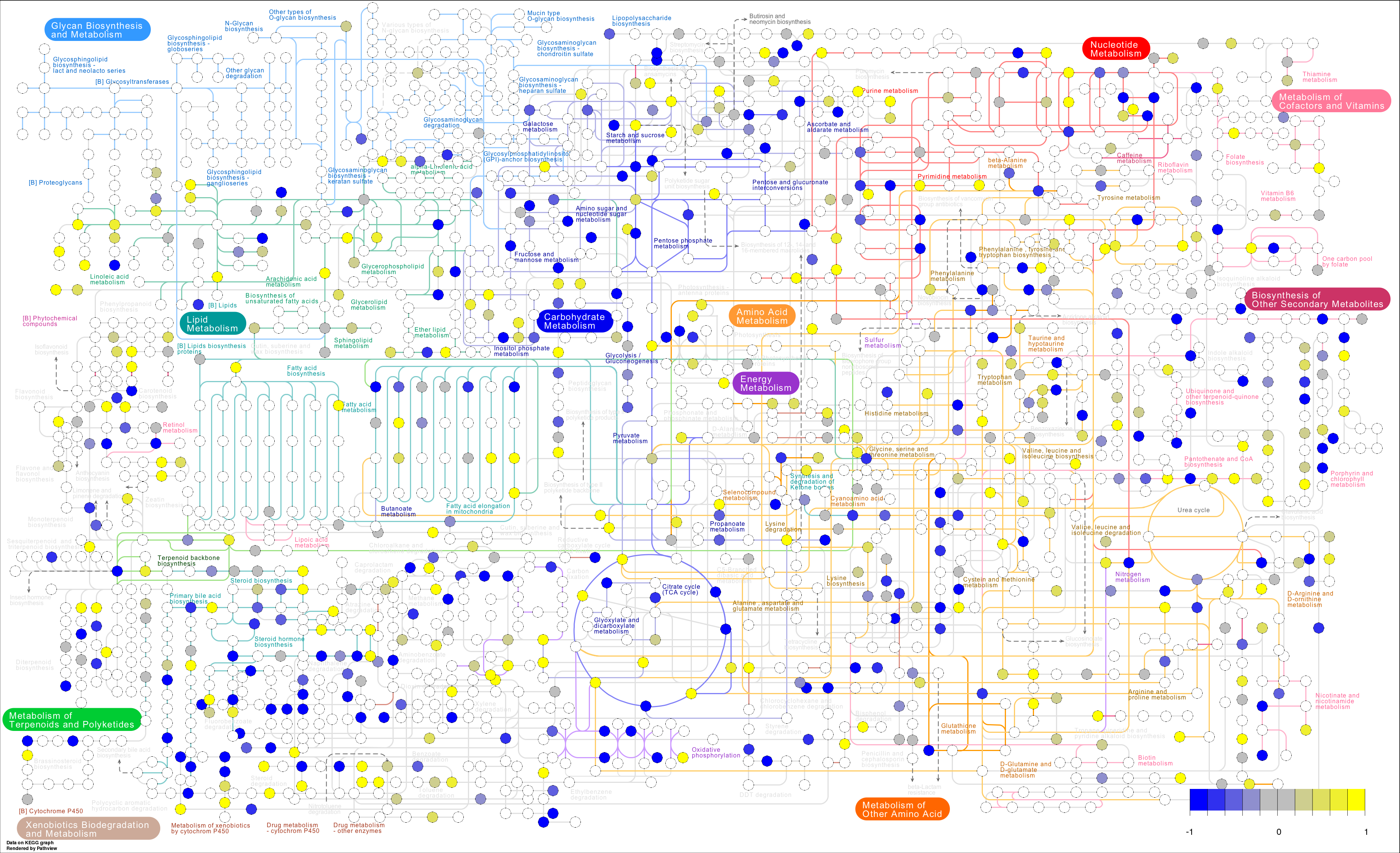
The [KEGG](http://www.genome.jp/kegg/) database is a useful repository of biochemical domain knowledge.
The following is an example of how to map changes in genes, proteins and metabolites on an organism specific basis to KEGG defined [biochemical pathways](http://www.genome.jp/kegg/pathway.html).
For this example we will use the R packages [pathview](http://bioconductor.org/packages/release/bioc/html/pathview.html), [KEGGREST](http://bioconductor.org/packages/2.12/bioc/html/KEGGREST.html) and [KEGGgraph](http://www.bioconductor.org/packages/release/bioc/html/KEGGgraph.html).
To generate a pathway enrichment visualization we minimally need a list of fold changes in biochemical components of interest (e.g. genes, proteins, metabolites).
We need to supply gene/protein and metabolite/compound fold changes separately as data.frames with rownames specifying database identifiers (see [pathview](http://pathview.r-forge.r-project.org/) for possible options).
This can be generated based on the output from statistical analysis used to identify any significantly differentially expressed species.
Lets create gene and metabolite data for a demonstration.
```{r,message=FALSE,warning=FALSE}
library(pathview)
metabolite.data<- data.frame(FC=sim.mol.data(mol.type="cpd", nmol=3000))
```
Lets take a look at the format of the metabolite inputs.
```{r}
head(metabolite.data)
```
Notice we have a single column data frame containing log fold changes with KEGG identifiers for the rownames. Next lets load the example gene data. For genes we can specify the organism of interest using the ```r 'species'``` argument. We can check for available organisms using the commands below.
```{r}
data(korg)
head(korg)
```
We can use the columns ```r 'scientific.name'``` or ```r 'common.name'``` to search for the ```r "kegg.code"``` for our organism of interest. Here is an example of how we can do this for *arabidopsis thaliana*.
```{r}
organism<-"arabidopsis thaliana"
matches<-unlist(sapply(1:ncol(korg),function(i) {agrep(organism,korg[,i])}))
(kegg.code<-korg[matches,1,drop=F])
```
```{r}
#load gene data
gene.data<- data.frame(FC=sim.mol.data(mol.type="gene", nmol=3000,species=kegg.code))
```
Lets take a look at the gene data.
```{r}
head(gene.data)
```
Looking at the rownames we can see that the identifiers are specific for arabidopsis thaliana. Using real data it is possible that we will need to translate identifiers to match the type used in pathview. Here are the different identifiers which can be supplied for metabolites.
```{r}
data(cpd.simtypes)
cpd.simtypes
```
Here are some possible options for gene identifiers.
```{r}
data(gene.idtype.list)
gene.idtype.list
```
We can optionally simulate data with with other identifiers by selecting the appropriate identifier type for the argument `id.type` in the function ```r "sim.mol.data"``` .
In the example data above we have the the logarithm of fold changes for `r nrow(metabolite.data)` metabolites and `r nrow(gene.data)` genes. Now that we have the data we can select some pathway of interest to map the fold changes to.
We could get this information from a pathway enrichment analysis. We would do this by testing if the significantly differential expressed metabolites or genes are enriched for some specific KEGG pathways of interest. Here are some tools to conduct enrichment analysis for genes and metabolites.
* [MBrole](http://csbg.cnb.csic.es/mbrole/) (metabolites)
* [MetaboAnalyst](http://www.metaboanalyst.ca/MetaboAnalyst/faces/Home.jsp) (metabolites)
* [David](http://david.abcc.ncifcrf.gov/) (genes)
* [IMPaLA](http://impala.molgen.mpg.de/) (genes and metabolites)
For the example below we will randomly select some KEGG pathways.
We can use the R package [KEGGREST](http://bioconductor.org/packages/2.12/bioc/html/KEGGREST.html) to get all KEGG pathway identifiers for ```r organism ```.
```{r,message=FALSE,warning=FALSE}
#get names of pathways to visualize
library(KEGGREST)
pathways<-keggList("pathway" ,kegg.code)
head(pathways)
```
Lets visualize changes in our genes and metabolites for ```r pathways[2] ``` which has the KEGG id ```r names(pathways)[2] ``` .
```{r,message=FALSE,warning=FALSE}
library(pathview)
map<-gsub("path:","",names(pathways)[2]) # remove 'path:'
pv.out <- pathview(gene.data = gene.data, cpd.data = metabolite.data, gene.idtype = "KEGG",
pathway.id = map, species = kegg.code, out.suffix = map,
keys.align = "y", kegg.native = T, match.data=T, key.pos = "topright")
plot.name<-paste(map,map,"png",sep=".")
```
If everything went as planned this generated a file named ```r plot.name``` mapped KEGG pathway.

We can take a look at the mappings made to this pathway.
```{r}
head(pv.out)
```
We can also display changes in genes/proteins and metabolites for multiple comparisons. To do this lets create some more artificial data and this time lets get protein information.
```{r}
metabolite.data2<- sim.mol.data(mol.type="cpd", nmol=3000,nexp=2)
head(metabolite.data2)
gene.data2<- sim.mol.data(mol.type="gene", nmol=3000,nexp=2,id.type="UNIPROT")
head(gene.data2)
```
Notice UNIPROT IDs do not map to ```r organism ```. We can check the available mappings by looking at the database of identifiers for ```r organism ``` org.At.tair.db. Lets instead map changes to a human pathway or KEGG code "hsa".
To do this we need to make sure we supply the correct ```r 'species' ``` and ```r 'gene.idtype'``` arguments. Next lets map changes in proteins and metabolites for the two comparisons to the pathway .
```{r, message=FALSE,warning=FALSE}
map<-gsub("path:ath","",names(pathways)[1]) # remove 'path:ath'
pv.out <- pathview(gene.data = gene.data2, cpd.data = metabolite.data2, gene.idtype = "UNIPROT",
pathway.id = map, species = "hsa", out.suffix = map,
keys.align = "y", kegg.native = T, match.data=T, key.pos = "topright")
plot.name<-paste(map,map,"multi","png",sep=".")
```
This should have generated an image file named ```r plot.name```.

We could also map metabolites on a large scale using `pathway.id= '01100'`.

```{r}
sessionInfo()
```
© Dmitry Grapov (2014)
================================================
FILE: Demos/Pathway Analysis/KEGG Pathway Enrichment.html
================================================
### Statistical Analysis
****
##### Next lets carry out a statistical analysis and summarise the changes between the sick and ghealthy groups. Below we identify significantly altered analytes using a basic t-test with adjustment for multiple hypotheses tested. We probably want to use more sophisticated and non-parametric tests for real applications.
```r
#get summaries and t-test stats
data.cube<-data.obj$normalized
data<-data.cube$data
meta<-data.cube$sample.meta[,"group",drop=FALSE]
#get summary
.summary<-stats.summary(data,comp.obj=meta,formula=colnames(meta),sigfigs=3,log=FALSE,rel=1,do.stats=TRUE)
```
```
## Generating data summary...
## Conducting tests...
## Conducting FDR corrections...
```
```r
stats.obj<-cbind(data.cube$variable.meta,.summary)
stats.obj %>% arrange(group_p.values) %>% head(.)
```
```
## ID description type
## 1 C00077 ornithine metabolite
## 2 C02477 tocopherol alpha metabolite
## 3 C00097 cysteine metabolite
## 4 C00031 glucose metabolite
## 5 C00170 5'-deoxy-5'-methylthioadenosine metabolite
## 6 C00385 xanthine metabolite
## healthy.mean.....std.dev sick.mean.....std.dev mean.sick_mean.healthy
## 1 7300 +/- 2900 3910 +/- 2100 0.54
## 2 1160 +/- 1400 2600 +/- 1200 2.24
## 3 5160 +/- 2500 8460 +/- 3400 1.64
## 4 335000 +/- 2e+05 144000 +/- 140000 0.43
## 5 216 +/- 83 355 +/- 160 1.64
## 6 574 +/- 350 1670 +/- 1500 2.91
## group_p.values group_adjusted.p.values group_q.values
## 1 9.433317e-06 0.001886663 0.000900412
## 2 1.505034e-04 0.007714558 0.003632462
## 3 1.507843e-04 0.007714558 0.003633836
## 4 1.542912e-04 0.007714558 0.003650646
## 5 2.004055e-04 0.008016221 0.003825749
## 6 3.909048e-04 0.013030159 0.006072846
```
```r
#write.csv(stats.obj,file="results/statistical_results.csv")
```
#### We can visualize the differences in means for the top most altered metabolite and protein as a box plot.
```r
top.met<-stats.obj %>% filter(type =="metabolite") %>%
arrange(group_p.values) %>% dplyr::select(ID) %>%
dplyr:: slice(.,1) %>% unlist(.) %>% as.character(.)
id<-as.character(stats.obj$ID) %in% top.met
tmp.data<-data.frame(data[,id,drop=FALSE],meta)
#make plot
ggplot(tmp.data,aes_string(x="group",y=colnames(tmp.data)[1],fill="group")) +
geom_boxplot() + ggtitle(as.character(stats.obj$description[id])) +ylab("")
```

```r
top.met<-stats.obj %>% filter(type =="protein") %>%
arrange(group_p.values) %>% dplyr::select(ID) %>%
dplyr:: slice(.,1) %>% unlist(.) %>% as.character(.)
id<-as.character(stats.obj$ID) %in% top.met
tmp.data<-data.frame(data[,id,drop=FALSE],meta)
#make plot
ggplot(tmp.data,aes_string(x="group",y=colnames(tmp.data)[1],fill="group")) +
geom_boxplot() + ggtitle(as.character(stats.obj$description[id])) +ylab("")
```

****
### Predictive Modeling
****
#### Next we can try a generate a non-linear multivarite classification model to identify important variables in our data. Below we will train and validate a random forest classifier. The full data set is split into 2/3 trainning and 1/3 test set while keeping the propotion of sick and healthy samples equivalent. The model is trained using 3-fold cross-validation repeated 3 times and the ```mtry``` parameter is optimized to maximize the are under the reciever operator characteristic curve (AUCROC).
```r
#create a classification model using random forests
#generate training/test set
set.seed(998)
data<-data.cube$data
inTraining <- createDataPartition(data.cube$sample.meta$group, p = 2/3, list = FALSE)
train.data <- data[ inTraining,]
test.data <- data[-inTraining,]
train.y <- data.cube$sample.meta$group[ inTraining] %>% droplevels()
test.y <- data.cube$sample.meta$group[ -inTraining] %>% droplevels()
#set model parameters
fitControl <- trainControl(## 10-fold CV
method = "repeatedcv",
number = 3,
## repeated ten times
repeats = 3,
classProbs = TRUE,
summaryFunction = twoClassSummary
)
#fit model to the training data
set.seed(825)
fit<- train(train.y ~ ., data = train.data,
method = "rf",
trControl = fitControl,
metric = "ROC",
tuneLength = 3
)
```
#### Below the optimal model is chosen while varying the ```mtry``` or the number of variables randomly sampled as candidates at each split.
```r
fit
```
```
## Random Forest
##
## 36 samples
## 199 predictors
## 2 classes: 'healthy', 'sick'
##
## No pre-processing
## Resampling: Cross-Validated (3 fold, repeated 3 times)
##
## Summary of sample sizes: 24, 24, 24, 24, 24, 24, ...
##
## Resampling results across tuning parameters:
##
## mtry ROC Sens Spec ROC SD Sens SD Spec SD
## 2 0.7870370 0.7222222 0.7777778 0.08098544 0.2041241 0.1666667
## 101 0.8549383 0.7777778 0.7592593 0.10090044 0.1443376 0.2060055
## 200 0.8750000 0.8333333 0.7222222 0.09107554 0.1178511 0.2204793
##
## ROC was used to select the optimal model using the largest value.
## The final value used for the model was mtry = 200.
```
#### Next we can evaluate the model performance based on predictions for the test set. We can also look at the ROC curve.
```r
#predict the test set
pred<-predict(fit,newdata=test.data)
prob<-predict(fit,newdata=test.data,type="prob")
obs<-test.y
table(pred,obs)
```
```
## obs
## pred healthy sick
## healthy 7 2
## sick 2 7
```
```r
#get performance stats
twoClassSummary(data=data.frame(obs,pred,prob),lev=levels(pred))
```
```
## ROC Sens Spec
## 0.9135802 0.7777778 0.7777778
```
#### We can also look at the ROC curve.
```r
x<-roc(obs,prob[,levels(pred)[1]],silent = TRUE)
plot(x)
```

```
##
## Call:
## roc.default(response = obs, predictor = prob[, levels(pred)[1]], silent = TRUE)
##
## Data: prob[, levels(pred)[1]] in 9 controls (obs healthy) > 9 cases (obs sick).
## Area under the curve: 0.9136
```
#### Having validated our model next we can look at the most important variables driving the classification. We can look at the differences in performance when each variable is randomly permuted or the VIP.
```r
#need to get variable names
vip<-varImp(fit)$importance # need to keep rownames
vip<-vip[order(vip[,1],decreasing=TRUE),,drop=FALSE][1:10,,drop=FALSE]
id<-colnames(train.data) %in% gsub('`','',rownames(vip))
tmp.data<-data.frame(importance=vip[,1],variable=factor(stats.obj$description[id],levels=stats.obj$description[id],ordered=FALSE))
#plot
ggplot(tmp.data, aes(x=variable,y=importance)) + geom_bar(stat="identity") + coord_flip()
```

```r
id<-as.character(stats.obj$description) %in% as.character(tmp.data[1,2])
tmp.data<-data.frame(data[,id,drop=FALSE],meta)
#make plot
ggplot(tmp.data,aes_string(x="group",y=colnames(tmp.data)[1],fill="group")) +
geom_boxplot() + ggtitle(as.character(stats.obj$description[id])) +ylab("")
```

****
### Functional Analysis
****
#### Finally we can identify enriched biological pathways based on the integrated changes in genes and proteins. [IMPaLA: Integrated Molecular Pathway Level Analysis](http://impala.molgen.mpg.de/) can be used to calculate enriched pathways in genes or proteins and metabolites.To do this we can querry the significantly alterd proteins and metabolites for enriched pathways (see `results/statistical_results_sig.csv`). We can view the full analysis results in `results/IMPaLA_results.csv`. next lets take an enriched pathway and fisualize the fold changes between sick and healthy in the enriched species.
```r
#format data to show fold changes in pathway
#get formatted data for pathview
library(KEGGREST)
library(pathview)
data<-stats.obj
#metabolite
met<-data %>% dplyr::filter(type =="metabolite") %>%
dplyr::select(ID,mean.sick_mean.healthy) %>%
mutate(FC=log(mean.sick_mean.healthy)) %>% dplyr::select(-mean.sick_mean.healthy)
#protein
prot<-data %>% dplyr::filter(type =="protein") %>%
dplyr::select(ID,mean.sick_mean.healthy) %>%
mutate(FC=log(mean.sick_mean.healthy)) %>% dplyr::select(-mean.sick_mean.healthy)
#set rownames
rownames(met)<-met[,1];met<-met[,-1,drop=FALSE]
rownames(prot)<-prot[,1];prot<-prot[,-1,drop=FALSE]
#select pathway to view
path<-"Glycolysis / Gluconeogenesis"
```
#### Lets take a looka at the Glycolysis / Gluconeogenesis pathway. Our data needs to be formatted as below. You can also take a look at the following more detailed example of [mapping fold changes to biochemical pathways](https://github.com/dgrapov/TeachingDemos/blob/master/Demos/Pathway%20Analysis/KEGG%20Pathway%20Enrichment.md).
#### Metabolite data showing KEGG ids and log fold change
```r
head(met)
```
```
## FC
## C00379 0.41871033
## C00385 1.06815308
## C00105 0.07696104
## C00299 -0.24846136
## C00366 0.33647224
## C00086 -0.05129329
```
#### Protein data showing the Entrez gene name and log fold changes
```r
head(prot)
```
```
## FC
## SPTAN1 -0.3424903
## CFH 0.1133287
## VPS13C 0.3148107
## XRCC6 1.0715836
## APOA1 -0.1392621
## SUPT16H 0.7129498
```
#### Next we need to get the pathway code for or pathway of interest.
```r
data(korg)
organism <- "homo sapiens"
matches <- unlist(sapply(1:ncol(korg), function(i) {
agrep(organism, korg[, i])
}))
(kegg.code <- korg[matches, 1, drop = F])
```
```
## kegg.code
## [1,] "hsa"
```
#### Now we can visualize the changes between sick and healthy in the Glycolysis / Gluconeogenesis pathway.
```r
setwd(wd)
pathways <- keggList("pathway", kegg.code)
#get code of our pathway of interest
map<-grepl(path,pathways) %>% pathways[.] %>% names(.) %>% gsub("path:","",.)
map
```
```
## [1] "hsa00010"
```
```r
#create image
setwd("report")
pv.out <- pathview(gene.data = prot, cpd.data = met, gene.idtype = "SYMBOL",
pathway.id = map, species = kegg.code, out.suffix = map, keys.align = "y",
kegg.native = T, match.data = T, key.pos = "topright")
```

****
#### This concludes this short tutorial. You may also find the following links useful.
* [Software tools](https://github.com/dgrapov)
* [More examples and demos](https://imdevsoftware.wordpress.com/)
© Dmitry Grapov (2015)
================================================
FILE: Demos/Data Analysis Workflow/results/IMPaLA_results.csv
================================================
pathway_name,pathway_source,num_overlapping_genes,overlapping_genes,num_all_pathway_genes,P_genes,Q_genes,num_overlapping_metabolites,overlapping_metabolites,num_all_pathway_metabolites,P_metabolites,Q_metabolites,P_joint,Q_joint
Metabolism,Reactome,3,GLS;IVD;ACSS2,1427 (1485),0.505,1,26,C00077;C00158;C00116;C00366;C00385;C00170;C01835;C00245;C00836;C00180;C00315;C00041;C00047;C00106;C00148;C00791;C00020;C00025;C00197;C00097;C00327;C00130;C00135;C03546;C00989;C00346,808 (1017),3.54E-13,8.03E-10,5.43E-12,5.61E-09
Transmembrane transport of small molecules,Reactome,0,,594 (623),1,1,16,C00077;C00106;C00116;C00148;C00245;C00158;C00791;C00020;C00025;C00097;C01571;C00366;C00315;C00041;C00047;C00135,204 (216),4.50E-13,8.03E-10,1.32E-11,6.85E-09
Metabolism of amino acids and derivatives,Reactome,2,IVD;GLS,145 (152),0.0292,1,14,C00077;C00148;C00245;C00791;C00020;C00197;C00025;C00170;C00097;C00315;C00327;C00041;C00047;C00135,181 (190),2.62E-11,1.87E-08,2.21E-11,7.61E-09
Metabolism of amino acids and derivatives,Wikipathways,0,,0 (0),1,1,14,C00077;C00148;C00245;C00791;C00020;C00197;C00025;C00170;C00097;C00315;C00327;C00041;C00047;C00135,174 (187),1.52E-11,1.36E-08,1.52E-11,1.36E-08
SLC-mediated transmembrane transport,Reactome,0,,261 (265),1,1,14,C00077;C00106;C00148;C00135;C00245;C00158;C00791;C00025;C00097;C01571;C00315;C00041;C00047;C00366,160 (165),4.77E-12,5.68E-09,1.29E-10,3.34E-08
Central carbon metabolism in cancer - Homo sapiens (human),KEGG,1,GLS,66 (67),0.116,1,8,C00158;C00148;C00031;C00197;C00025;C00097;C00041;C00135,37 (37),2.36E-10,9.37E-08,6.92E-10,1.43E-07
ABC transporters - Homo sapiens (human),KEGG,0,,44 (44),1,1,12,C00077;C00116;C00148;C00245;C00379;C00031;C00025;C00047;C00315;C00041;C01835;C00135,123 (123),6.60E-11,3.37E-08,1.61E-09,2.39E-07
Amino acid transport across the plasma membrane,Reactome,0,,31 (31),1,1,8,C00077;C00148;C00245;C00025;C00097;C00041;C00047;C00135,32 (32),6.61E-11,3.37E-08,1.62E-09,2.39E-07
Transport of glucose and other sugars_ bile salts and organic acids_ metal ions and amine compounds,Reactome,0,,98 (101),1,1,10,C00158;C00148;C00366;C00791;C00245;C00097;C00315;C00041;C00047;C00135,78 (83),2.28E-10,9.37E-08,5.30E-09,6.86E-07
Urea cycle and metabolism of arginine_ proline_ glutamate_ aspartate and asparagine,EHMN,1,GLS,105 (107),0.178,1,11,C00077;C00148;C00020;C00025;C00170;C00097;C00315;C00327;C00041;C00047;C00989,125 (125),1.52E-09,4.53E-07,6.24E-09,7.18E-07
tRNA charging,HumanCyc,0,,41 (44),1,1,7,C00148;C00020;C00025;C00097;C00041;C00047;C00135,24 (24),3.55E-10,1.27E-07,8.07E-09,7.78E-07
Class I MHC mediated antigen processing & presentation,Reactome,2,SEC24C;SEC13,208 (224),0.0561,1,7,C00148;C00020;C00025;C00097;C00041;C00047;C00135,35 (35),6.48E-09,1.54E-06,8.27E-09,7.78E-07
Glucose Homeostasis,Wikipathways,0,,0 (0),1,1,6,C00077;C00116;C00031;C00327;C00047;C00135,21 (21),8.50E-09,1.78E-06,8.50E-09,1.78E-06
Amino acid and oligopeptide SLC transporters,Reactome,0,,49 (49),1,1,8,C00077;C00148;C00245;C00025;C00097;C00041;C00047;C00135,45 (45),1.26E-09,4.10E-07,2.71E-08,2.34E-06
Transport of inorganic cations/anions and amino acids/oligopeptides,Reactome,0,,94 (95),1,1,8,C00077;C00148;C00245;C00025;C00097;C00041;C00047;C00135,48 (48),2.17E-09,5.97E-07,4.55E-08,3.63E-06
Amino acid synthesis and interconversion (transamination),Reactome,1,GLS,17 (17),0.0311,1,6,C00077;C00148;C00020;C00197;C00025;C00041,32 (32),1.33E-07,1.83E-05,8.42E-08,6.22E-06
Adaptive Immune System,Reactome,3,SEC24C;EVL;SEC13,558 (608),0.0819,1,7,C00148;C00020;C00025;C00097;C00041;C00047;C00135,48 (48),6.59E-08,1.21E-05,1.08E-07,7.46E-06
Endosomal/Vacuolar pathway,Reactome,0,,12 (12),1,1,6,C00148;C00025;C00097;C00041;C00047;C00135,20 (20),6.10E-09,1.54E-06,1.22E-07,7.86E-06
Proton/oligonucleotide cotransporters,Reactome,0,,4 (4),1,1,6,C00148;C00025;C00097;C00041;C00047;C00135,21 (21),8.50E-09,1.78E-06,1.66E-07,1.01E-05
Transport of inorganic cations-anions and amino acids-oligopeptides,Wikipathways,0,,0 (0),1,1,6,C00148;C00025;C00097;C00041;C00047;C00135,31 (32),1.09E-07,1.56E-05,1.09E-07,1.56E-05
γ-glutamyl cycle,HumanCyc,0,,11 (12),1,1,7,C00077;C00148;C00025;C00097;C00041;C00047;C00135,43 (47),2.97E-08,5.89E-06,5.44E-07,3.13E-05
Antigen processing-Cross presentation,Reactome,0,,32 (32),1,1,6,C00148;C00025;C00097;C00041;C00047;C00135,29 (29),7.11E-08,1.21E-05,1.24E-06,6.42E-05
leukotriene biosynthesis,HumanCyc,0,,6 (7),1,1,6,C00148;C00025;C00097;C00041;C00047;C00135,29 (30),7.11E-08,1.21E-05,1.24E-06,6.42E-05
tRNA Aminoacylation,Wikipathways,0,,0 (0),1,1,7,C00148;C00020;C00025;C00097;C00041;C00047;C00135,65 (65),5.67E-07,6.53E-05,5.67E-07,6.53E-05
Glutathione synthesis and recycling,Reactome,0,,14 (17),1,1,6,C00148;C00025;C00097;C00041;C00047;C00135,30 (31),8.83E-08,1.37E-05,1.52E-06,7.16E-05
Urea cycle and metabolism of amino groups,Wikipathways,0,,20 (20),1,1,6,C00077;C00148;C00791;C00025;C00315;C00327,30 (30),8.83E-08,1.37E-05,1.52E-06,7.16E-05
Na+/Cl- dependent neurotransmitter transporters,Reactome,0,,19 (19),1,1,6,C00148;C00245;C00097;C00041;C00047;C00135,31 (31),1.09E-07,1.56E-05,1.85E-06,8.35E-05
Phase II conjugation,Wikipathways,0,,0 (0),1,1,8,C00148;C00020;C00025;C00097;C00180;C00041;C00047;C00135,102 (115),9.38E-07,9.57E-05,9.38E-07,9.57E-05
Nucleotide Metabolism,Wikipathways,0,,19 (19),1,1,5,C00077;C00385;C00130;C00366;C00315,17 (18),1.44E-07,1.90E-05,2.41E-06,0.000104
Amine compound SLC transporters,Reactome,0,,30 (31),1,1,6,C00148;C00245;C00097;C00041;C00047;C00135,35 (35),2.35E-07,2.89E-05,3.82E-06,0.000152
S-methyl-5-thio-α-D-ribose 1-phosphate degradation,HumanCyc,0,,4 (4),1,1,6,C00148;C00025;C00097;C00041;C00047;C00135,35 (35),2.35E-07,2.89E-05,3.82E-06,0.000152
Glutathione conjugation,Reactome,0,,35 (38),1,1,6,C00148;C00025;C00097;C00041;C00047;C00135,38 (41),3.92E-07,4.67E-05,6.18E-06,0.000237
Immune System,Reactome,4,SEC24C;EVL;XRCC6;SEC13,994 (1069),0.106,1,7,C00148;C00020;C00025;C00097;C00041;C00047;C00135,87 (103),4.20E-06,0.000273,6.98E-06,0.000258
Glycine_ serine_ alanine and threonine metabolism,EHMN,1,GLOD4,80 (80),0.139,1,7,C00077;C00020;C00197;C00025;C00097;C00041;C00047,88 (88),4.54E-06,0.000289,9.61E-06,0.000311
Cytosolic tRNA aminoacylation,Reactome,0,,26 (29),1,1,7,C00148;C00020;C00025;C00097;C00041;C00047;C00135,66 (66),6.30E-07,6.62E-05,9.63E-06,0.000311
Mitochondrial tRNA aminoacylation,Reactome,0,,23 (23),1,1,7,C00148;C00020;C00025;C00097;C00041;C00047;C00135,66 (66),6.30E-07,6.62E-05,9.63E-06,0.000311
tRNA Aminoacylation,Reactome,0,,45 (48),1,1,7,C00148;C00020;C00025;C00097;C00041;C00047;C00135,66 (66),6.30E-07,6.62E-05,9.63E-06,0.000311
Metabolism of nucleotides,Wikipathways,0,,0 (0),1,1,7,C00106;C00366;C00385;C00025;C00020;C00130;C00041,97 (111),8.73E-06,0.000528,8.73E-06,0.000528
Chloramphenicol Action Pathway,SMPDB,0,,0 (0),1,1,4,C00020;C00148;C00041;C00135,20 (20),1.55E-05,0.000609,1.55E-05,0.000609
Roxithromycin Action Pathway,SMPDB,0,,0 (0),1,1,4,C00020;C00148;C00041;C00135,20 (20),1.55E-05,0.000609,1.55E-05,0.000609
Josamycin Action Pathway,SMPDB,0,,0 (0),1,1,4,C00020;C00148;C00041;C00135,20 (20),1.55E-05,0.000609,1.55E-05,0.000609
Methacycline Action Pathway,SMPDB,0,,0 (0),1,1,4,C00020;C00148;C00041;C00135,20 (20),1.55E-05,0.000609,1.55E-05,0.000609
Rolitetracycline Action Pathway,SMPDB,0,,0 (0),1,1,4,C00020;C00148;C00041;C00135,20 (20),1.55E-05,0.000609,1.55E-05,0.000609
Streptomycin Action Pathway,SMPDB,0,,0 (0),1,1,4,C00020;C00148;C00041;C00135,20 (20),1.55E-05,0.000609,1.55E-05,0.000609
Spectinomycin Action Pathway,SMPDB,0,,0 (0),1,1,4,C00020;C00148;C00041;C00135,20 (20),1.55E-05,0.000609,1.55E-05,0.000609
Kanamycin Action Pathway,SMPDB,0,,0 (0),1,1,4,C00020;C00148;C00041;C00135,20 (20),1.55E-05,0.000609,1.55E-05,0.000609
Gentamicin Action Pathway,SMPDB,0,,0 (0),1,1,4,C00020;C00148;C00041;C00135,20 (20),1.55E-05,0.000609,1.55E-05,0.000609
Netilmicin Action Pathway,SMPDB,0,,0 (0),1,1,4,C00020;C00148;C00041;C00135,20 (20),1.55E-05,0.000609,1.55E-05,0.000609
Neomycin Action Pathway,SMPDB,0,,0 (0),1,1,4,C00020;C00148;C00041;C00135,20 (20),1.55E-05,0.000609,1.55E-05,0.000609
Tobramycin Action Pathway,SMPDB,0,,0 (0),1,1,4,C00020;C00148;C00041;C00135,20 (20),1.55E-05,0.000609,1.55E-05,0.000609
Paromomycin Action Pathway,SMPDB,0,,0 (0),1,1,4,C00020;C00148;C00041;C00135,20 (20),1.55E-05,0.000609,1.55E-05,0.000609
Minocycline Action Pathway,SMPDB,0,,0 (0),1,1,4,C00020;C00148;C00041;C00135,20 (20),1.55E-05,0.000609,1.55E-05,0.000609
Tetracycline Action Pathway,SMPDB,0,,0 (0),1,1,4,C00020;C00148;C00041;C00135,20 (20),1.55E-05,0.000609,1.55E-05,0.000609
Lincomycin Action Pathway,SMPDB,0,,0 (0),1,1,4,C00020;C00148;C00041;C00135,20 (20),1.55E-05,0.000609,1.55E-05,0.000609
Clindamycin Action Pathway,SMPDB,0,,0 (0),1,1,4,C00020;C00148;C00041;C00135,20 (20),1.55E-05,0.000609,1.55E-05,0.000609
Azithromycin Action Pathway,SMPDB,0,,0 (0),1,1,4,C00020;C00148;C00041;C00135,20 (20),1.55E-05,0.000609,1.55E-05,0.000609
Arbekacin Action Pathway,SMPDB,0,,0 (0),1,1,4,C00020;C00148;C00041;C00135,20 (20),1.55E-05,0.000609,1.55E-05,0.000609
Tigecycline Action Pathway,SMPDB,0,,0 (0),1,1,4,C00020;C00148;C00041;C00135,20 (20),1.55E-05,0.000609,1.55E-05,0.000609
Erythromycin Action Pathway,SMPDB,0,,0 (0),1,1,4,C00020;C00148;C00041;C00135,20 (20),1.55E-05,0.000609,1.55E-05,0.000609
Amikacin Action Pathway,SMPDB,0,,0 (0),1,1,4,C00020;C00148;C00041;C00135,20 (20),1.55E-05,0.000609,1.55E-05,0.000609
Clomocycline Action Pathway,SMPDB,0,,0 (0),1,1,4,C00020;C00148;C00041;C00135,20 (20),1.55E-05,0.000609,1.55E-05,0.000609
Doxycycline Action Pathway,SMPDB,0,,0 (0),1,1,4,C00020;C00148;C00041;C00135,20 (20),1.55E-05,0.000609,1.55E-05,0.000609
Demeclocycline Action Pathway,SMPDB,0,,0 (0),1,1,4,C00020;C00148;C00041;C00135,20 (20),1.55E-05,0.000609,1.55E-05,0.000609
Oxytetracycline Action Pathway,SMPDB,0,,0 (0),1,1,4,C00020;C00148;C00041;C00135,20 (20),1.55E-05,0.000609,1.55E-05,0.000609
Lymecycline Action Pathway,SMPDB,0,,0 (0),1,1,4,C00020;C00148;C00041;C00135,20 (20),1.55E-05,0.000609,1.55E-05,0.000609
Telithromycin Action Pathway,SMPDB,0,,0 (0),1,1,4,C00020;C00148;C00041;C00135,20 (20),1.55E-05,0.000609,1.55E-05,0.000609
Clarithromycin Action Pathway,SMPDB,0,,0 (0),1,1,4,C00020;C00148;C00041;C00135,20 (20),1.55E-05,0.000609,1.55E-05,0.000609
Troleandomycin Action Pathway,SMPDB,0,,0 (0),1,1,4,C00020;C00148;C00041;C00135,20 (20),1.55E-05,0.000609,1.55E-05,0.000609
Protein digestion and absorption - Homo sapiens (human),KEGG,0,,87 (89),1,1,6,C00148;C00025;C00097;C00041;C00047;C00135,47 (47),1.45E-06,0.000144,2.09E-05,0.000657
Argininemia,SMPDB,0,,13 (13),1,1,5,C00077;C00327;C00041;C00020;C00025,27 (27),1.77E-06,0.000151,2.52E-05,0.000669
Citrullinemia Type I,SMPDB,0,,13 (13),1,1,5,C00077;C00327;C00041;C00020;C00025,27 (27),1.77E-06,0.000151,2.52E-05,0.000669
Carbamoyl Phosphate Synthetase Deficiency,SMPDB,0,,13 (13),1,1,5,C00077;C00327;C00041;C00020;C00025,27 (27),1.77E-06,0.000151,2.52E-05,0.000669
Argininosuccinic Aciduria,SMPDB,0,,13 (13),1,1,5,C00077;C00327;C00041;C00020;C00025,27 (27),1.77E-06,0.000151,2.52E-05,0.000669
Urea Cycle,SMPDB,0,,13 (13),1,1,5,C00077;C00327;C00041;C00020;C00025,27 (27),1.77E-06,0.000151,2.52E-05,0.000669
Ornithine Transcarbamylase Deficiency (OTC Deficiency),SMPDB,0,,13 (13),1,1,5,C00077;C00327;C00041;C00020;C00025,27 (27),1.77E-06,0.000151,2.52E-05,0.000669
Aminoacyl-tRNA biosynthesis - Homo sapiens (human),KEGG,0,,66 (66),1,1,6,C00148;C00025;C00097;C00041;C00047;C00135,52 (52),2.67E-06,0.000222,3.70E-05,0.000956
Gene Expression,Reactome,3,EEF1D;HNRNPF;RPL9,1182 (1251),0.379,1,7,C00148;C00020;C00025;C00097;C00041;C00047;C00135,97 (104),8.73E-06,0.000528,4.50E-05,0.000991
Phase II conjugation,Reactome,0,,94 (102),1,1,8,C00148;C00020;C00025;C00097;C00180;C00041;C00047;C00135,122 (145),3.69E-06,0.000244,4.98E-05,0.000991
Defective AHCY causes Hypermethioninemia with S-adenosylhomocysteine hydrolase deficiency (HMAHCHD),Reactome,0,,94 (102),1,1,8,C00148;C00020;C00025;C00097;C00180;C00041;C00047;C00135,122 (145),3.69E-06,0.000244,4.98E-05,0.000991
Defective GCLC causes Hemolytic anemia due to gamma-glutamylcysteine synthetase deficiency (HAGGSD),Reactome,0,,94 (102),1,1,8,C00148;C00020;C00025;C00097;C00180;C00041;C00047;C00135,122 (145),3.69E-06,0.000244,4.98E-05,0.000991
Defective UGT1A1 causes hyperbilirubinemia,Reactome,0,,94 (102),1,1,8,C00148;C00020;C00025;C00097;C00180;C00041;C00047;C00135,122 (145),3.69E-06,0.000244,4.98E-05,0.000991
Defective GSS causes Glutathione synthetase deficiency (GSS deficiency),Reactome,0,,94 (102),1,1,8,C00148;C00020;C00025;C00097;C00180;C00041;C00047;C00135,122 (145),3.69E-06,0.000244,4.98E-05,0.000991
Defective GGT1 causes Glutathionuria (GLUTH),Reactome,0,,94 (102),1,1,8,C00148;C00020;C00025;C00097;C00180;C00041;C00047;C00135,122 (145),3.69E-06,0.000244,4.98E-05,0.000991
Defective UGT1A4 causes hyperbilirubinemia,Reactome,0,,94 (102),1,1,8,C00148;C00020;C00025;C00097;C00180;C00041;C00047;C00135,122 (145),3.69E-06,0.000244,4.98E-05,0.000991
Defective MAT1A causes Methionine adenosyltransferase deficiency (MATD),Reactome,0,,94 (102),1,1,8,C00148;C00020;C00025;C00097;C00180;C00041;C00047;C00135,122 (145),3.69E-06,0.000244,4.98E-05,0.000991
Defective SLC35D1 causes Schneckenbecken dysplasia (SCHBCKD),Reactome,0,,94 (102),1,1,8,C00148;C00020;C00025;C00097;C00180;C00041;C00047;C00135,122 (145),3.69E-06,0.000244,4.98E-05,0.000991
Defective TPMT causes Thiopurine S-methyltransferase deficiency (TPMT deficiency),Reactome,0,,94 (102),1,1,8,C00148;C00020;C00025;C00097;C00180;C00041;C00047;C00135,122 (145),3.69E-06,0.000244,4.98E-05,0.000991
Defective OPLAH causes 5-oxoprolinase deficiency (OPLAHD),Reactome,0,,94 (102),1,1,8,C00148;C00020;C00025;C00097;C00180;C00041;C00047;C00135,122 (145),3.69E-06,0.000244,4.98E-05,0.000991
FoxO signaling pathway - Homo sapiens (human),KEGG,0,,127 (134),1,1,3,C00020;C00031;C00025,5 (5),4.73E-06,0.000296,6.27E-05,0.00122
Glycolysis / Gluconeogenesis - Homo sapiens (human),KEGG,3,ADH5;PGK2;ACSS2,66 (67),0.000232,0.303,2,C00031;C00197,31 (31),0.0253,0.229,7.68E-05,0.00147
Metabolism of proteins,Reactome,5,EEF1D;EIF5A2;SEC24C;SEC13;RPL9,662 (693),0.00618,1,6,C00020;C00025;C00170;C01571;C06423;C00315,148 (163),0.000998,0.0166,8.01E-05,0.00151
Arginine and proline metabolism - Homo sapiens (human),KEGG,1,GLS,60 (61),0.106,1,6,C00077;C00148;C00791;C00025;C00315;C00327,91 (91),7.00E-05,0.00227,9.49E-05,0.00175
Disease,Reactome,4,SEC24C;XRCC6;SEC13;ACSS2,1747 (1852),0.412,1,14,C00077;C00158;C00148;C00020;C00197;C01835;C00025;C00097;C00180;C00315;C00327;C00041;C00047;C00135,533 (699),2.61E-05,0.00099,0.000133,0.00242
Biological oxidations,Reactome,1,ACSS2,174 (189),0.278,1,9,C00148;C00020;C00025;C00097;C00180;C00315;C00041;C00047;C00135,220 (278),3.96E-05,0.00147,0.000137,0.00244
One carbon donor,Wikipathways,0,,1 (1),1,1,4,C00077;C00245;C00097;C00315,19 (23),1.25E-05,0.000609,0.000153,0.00265
purine nucleotides degradation,HumanCyc,0,,12 (12),1,1,4,C00385;C00020;C00130;C00366,19 (19),1.25E-05,0.000609,0.000153,0.00265
Amino acid conjugation of benzoic acid,Wikipathways,1,ACSS2,4 (4),0.00741,1,2,C00020;C00180,9 (9),0.00219,0.0312,0.000195,0.00331
Urea cycle,Reactome,0,,9 (10),1,1,4,C00077;C00327;C00020;C00025,21 (21),1.91E-05,0.00074,0.000226,0.00378
Taurine and hypotaurine metabolism - Homo sapiens (human),KEGG,0,,10 (10),1,1,4,C00041;C00245;C00097;C00025,22 (22),2.32E-05,0.000889,0.00027,0.00444
Metabolism of carbohydrates,Wikipathways,0,,0 (0),1,1,5,C00158;C00020;C00197;C01835;C00025,66 (69),0.000157,0.00459,0.000157,0.00459
Metabolism of nucleotides,Reactome,0,,81 (83),1,1,7,C00106;C00366;C00385;C00025;C00020;C00130;C00041,122 (135),3.95E-05,0.00147,0.00044,0.00712
Gamma carboxylation_ hypusine formation and arylsulfatase activation,Reactome,1,EIF5A2,35 (35),0.0631,1,3,C00020;C00170;C00315,23 (23),0.000758,0.0135,0.000524,0.00725
Hyperornithinemia with gyrate atrophy (HOGA),SMPDB,0,,20 (20),1,1,5,C00327;C00077;C00148;C00020;C00025,52 (52),4.94E-05,0.00163,0.000539,0.00725
Creatine deficiency_ guanidinoacetate methyltransferase deficiency,SMPDB,0,,20 (20),1,1,5,C00327;C00077;C00148;C00020;C00025,52 (52),4.94E-05,0.00163,0.000539,0.00725
L-arginine:glycine amidinotransferase deficiency,SMPDB,0,,20 (20),1,1,5,C00327;C00077;C00148;C00020;C00025,52 (52),4.94E-05,0.00163,0.000539,0.00725
Hyperornithinemia-hyperammonemia-homocitrullinuria [HHH-syndrome],SMPDB,0,,20 (20),1,1,5,C00327;C00077;C00148;C00020;C00025,52 (52),4.94E-05,0.00163,0.000539,0.00725
Guanidinoacetate Methyltransferase Deficiency (GAMT Deficiency),SMPDB,0,,20 (20),1,1,5,C00327;C00077;C00148;C00020;C00025,52 (52),4.94E-05,0.00163,0.000539,0.00725
Prolinemia Type II,SMPDB,0,,20 (20),1,1,5,C00327;C00077;C00148;C00020;C00025,52 (52),4.94E-05,0.00163,0.000539,0.00725
Prolidase Deficiency (PD),SMPDB,0,,20 (20),1,1,5,C00327;C00077;C00148;C00020;C00025,52 (52),4.94E-05,0.00163,0.000539,0.00725
Hyperprolinemia Type I,SMPDB,0,,20 (20),1,1,5,C00327;C00077;C00148;C00020;C00025,52 (52),4.94E-05,0.00163,0.000539,0.00725
Hyperprolinemia Type II,SMPDB,0,,20 (20),1,1,5,C00327;C00077;C00148;C00020;C00025,52 (52),4.94E-05,0.00163,0.000539,0.00725
Ornithine Aminotransferase Deficiency (OAT Deficiency),SMPDB,0,,20 (20),1,1,5,C00327;C00077;C00148;C00020;C00025,52 (52),4.94E-05,0.00163,0.000539,0.00725
Arginine: Glycine Amidinotransferase Deficiency (AGAT Deficiency),SMPDB,0,,20 (20),1,1,5,C00327;C00077;C00148;C00020;C00025,52 (52),4.94E-05,0.00163,0.000539,0.00725
Arginine and Proline Metabolism,SMPDB,0,,20 (20),1,1,5,C00327;C00077;C00148;C00020;C00025,52 (52),4.94E-05,0.00163,0.000539,0.00725
molybdenum cofactor biosynthesis,HumanCyc,0,,4 (4),1,1,3,C00020;C00041;C00097,10 (13),5.52E-05,0.00181,0.000596,0.00791
Metabolic disorders of biological oxidation enzymes,Reactome,1,ACSS2,584 (641),0.672,1,10,C00077;C00148;C00020;C00025;C00097;C00180;C00315;C00041;C00047;C00135,305 (382),9.00E-05,0.00285,0.000649,0.0085
Metabolism of water-soluble vitamins and cofactors,Wikipathways,0,,0 (0),1,1,5,C00020;C00041;C00047;C00097;C00025,83 (96),0.000462,0.00988,0.000462,0.00988
urate biosynthesis/inosine 5_-phosphate degradation,HumanCyc,0,,6 (6),1,1,3,C00385;C00130;C00366,11 (11),7.55E-05,0.00241,0.000792,0.0101
Glucose-Alanine Cycle,SMPDB,0,,8 (8),1,1,3,C00031;C00041;C00025,11 (11),7.55E-05,0.00241,0.000792,0.0101
Alanine_ aspartate and glutamate metabolism - Homo sapiens (human),KEGG,1,GLS,35 (35),0.0631,1,3,C00158;C00041;C00025,28 (28),0.00136,0.0214,0.000892,0.0113
Synthesis_ Secretion_ and Deacylation of Ghrelin,Wikipathways,0,,0 (0),1,1,2,C01571;C06423,5 (5),0.000621,0.0121,0.000621,0.0121
triacylglycerol degradation,HumanCyc,0,,15 (15),1,1,4,C01571;C00116;C06423;C01601,32 (56),0.000108,0.00334,0.00109,0.0134
Purine catabolism,Reactome,0,,11 (11),1,1,4,C00385;C00020;C00130;C00366,32 (32),0.000108,0.00334,0.00109,0.0134
COPII (Coat Protein 2) Mediated Vesicle Transport,Reactome,2,SEC24C;SEC13,9 (10),0.000117,0.228,0,,3 (3),1,1,0.00118,0.0142
ER to Golgi Transport,Reactome,2,SEC24C;SEC13,9 (10),0.000117,0.228,0,,3 (3),1,1,0.00118,0.0142
Gluconeogenesis,Reactome,0,,32 (33),1,1,4,C00158;C00020;C00197;C00025,33 (33),0.000122,0.00375,0.00122,0.0145
adenosine nucleotides degradation,HumanCyc,0,,9 (9),1,1,3,C00385;C00020;C00366,13 (13),0.000129,0.00395,0.00129,0.0151
SREBP signalling,Wikipathways,2,SEC24C;SEC13,60 (60),0.00543,1,1,C00031,3 (5),0.024,0.219,0.0013,0.0151
Hypoacetylaspartia,SMPDB,0,,14 (14),1,1,4,C00020;C00327;C00130;C00025,34 (34),0.000137,0.00408,0.00136,0.0153
Canavan Disease,SMPDB,0,,14 (14),1,1,4,C00020;C00327;C00130;C00025,34 (34),0.000137,0.00408,0.00136,0.0153
Aspartate Metabolism,SMPDB,0,,14 (14),1,1,4,C00020;C00327;C00130;C00025,34 (34),0.000137,0.00408,0.00136,0.0153
[2Fe-2S] iron-sulfur cluster biosynthesis,HumanCyc,0,,0 (0),1,1,2,C00041;C00097,6 (6),0.000927,0.0155,0.000927,0.0155
Purine metabolism,Reactome,0,,34 (36),1,1,5,C00385;C00020;C00130;C00366;C00025,66 (67),0.000157,0.00459,0.00153,0.017
Trans-sulfuration pathway,Wikipathways,0,,10 (10),1,1,3,C00245;C00097;C00025,14 (14),0.000164,0.00476,0.00159,0.0175
GPCR downstream signaling,Wikipathways,0,,0 (0),1,1,5,C00077;C00020;C00116;C00047;C00025,101 (121),0.00114,0.0183,0.00114,0.0183
Post-translational protein modification,Reactome,3,EIF5A2;SEC24C;SEC13,281 (290),0.0144,1,4,C00020;C00025;C00170;C00315,113 (126),0.0122,0.129,0.00169,0.0184
glutamine degradation/glutamate biosynthesis,HumanCyc,1,GLS,3 (3),0.00556,1,1,C00025,4 (4),0.0319,0.26,0.00171,0.0184
Synthesis_ secretion_ and deacylation of Ghrelin,Reactome,0,,8 (9),1,1,2,C01571;C06423,3 (3),0.000188,0.00542,0.0018,0.0192
guanosine ribonucleotides de novo biosynthesis,HumanCyc,0,,13 (13),1,1,3,C00020;C00130;C00025,15 (15),0.000204,0.00577,0.00193,0.0201
Molybdenum cofactor biosynthesis,Reactome,0,,6 (6),1,1,3,C00020;C00041;C00097,15 (20),0.000204,0.00577,0.00193,0.0201
Glutathione metabolism - Homo sapiens (human),KEGG,0,,51 (51),1,1,4,C00077;C00025;C00097;C00315,38 (38),0.000213,0.006,0.00202,0.0201
Xanthine Dehydrogenase Deficiency (Xanthinuria),SMPDB,0,,37 (37),1,1,5,C00385;C00020;C00130;C00025;C00366,72 (72),0.000237,0.00601,0.00222,0.0201
Adenylosuccinate Lyase Deficiency,SMPDB,0,,37 (37),1,1,5,C00385;C00020;C00130;C00025;C00366,72 (72),0.000237,0.00601,0.00222,0.0201
AICA-Ribosiduria,SMPDB,0,,37 (37),1,1,5,C00385;C00020;C00130;C00025;C00366,72 (72),0.000237,0.00601,0.00222,0.0201
Adenine phosphoribosyltransferase deficiency (APRT),SMPDB,0,,37 (37),1,1,5,C00385;C00020;C00130;C00025;C00366,72 (72),0.000237,0.00601,0.00222,0.0201
Purine Metabolism,SMPDB,0,,37 (37),1,1,5,C00385;C00020;C00130;C00025;C00366,72 (72),0.000237,0.00601,0.00222,0.0201
Molybdenum Cofactor Deficiency,SMPDB,0,,37 (37),1,1,5,C00385;C00020;C00130;C00025;C00366,72 (72),0.000237,0.00601,0.00222,0.0201
Adenosine Deaminase Deficiency,SMPDB,0,,37 (37),1,1,5,C00385;C00020;C00130;C00025;C00366,72 (72),0.000237,0.00601,0.00222,0.0201
Gout or Kelley-Seegmiller Syndrome,SMPDB,0,,37 (37),1,1,5,C00385;C00020;C00130;C00025;C00366,72 (72),0.000237,0.00601,0.00222,0.0201
Lesch-Nyhan Syndrome (LNS),SMPDB,0,,37 (37),1,1,5,C00385;C00020;C00130;C00025;C00366,72 (72),0.000237,0.00601,0.00222,0.0201
Xanthinuria type I,SMPDB,0,,37 (37),1,1,5,C00385;C00020;C00130;C00025;C00366,72 (72),0.000237,0.00601,0.00222,0.0201
Xanthinuria type II,SMPDB,0,,37 (37),1,1,5,C00385;C00020;C00130;C00025;C00366,72 (72),0.000237,0.00601,0.00222,0.0201
Purine Nucleoside Phosphorylase Deficiency,SMPDB,0,,37 (37),1,1,5,C00385;C00020;C00130;C00025;C00366,72 (72),0.000237,0.00601,0.00222,0.0201
Mitochondrial DNA depletion syndrome,SMPDB,0,,37 (37),1,1,5,C00385;C00020;C00130;C00025;C00366,72 (72),0.000237,0.00601,0.00222,0.0201
Myoadenylate deaminase deficiency,SMPDB,0,,37 (37),1,1,5,C00385;C00020;C00130;C00025;C00366,72 (72),0.000237,0.00601,0.00222,0.0201
sphingosine and sphingosine-1-phosphate metabolism,HumanCyc,0,,9 (9),1,1,4,C01571;C06423;C01601;C00346,40 (59),0.000261,0.00657,0.00242,0.0217
acetate conversion to acetyl-CoA,HumanCyc,1,ACSS2,3 (3),0.00556,1,1,C00020,6 (6),0.0475,0.336,0.00244,0.0217
Methionine Adenosyltransferase Deficiency,SMPDB,0,,19 (20),1,1,4,C00020;C00170;C00097;C00315,41 (42),0.000288,0.00685,0.00263,0.0217
Glycine N-methyltransferase Deficiency,SMPDB,0,,19 (20),1,1,4,C00020;C00170;C00097;C00315,41 (42),0.000288,0.00685,0.00263,0.0217
Hypermethioninemia,SMPDB,0,,19 (20),1,1,4,C00020;C00170;C00097;C00315,41 (42),0.000288,0.00685,0.00263,0.0217
Methylenetetrahydrofolate Reductase Deficiency (MTHFRD),SMPDB,0,,19 (20),1,1,4,C00020;C00170;C00097;C00315,41 (42),0.000288,0.00685,0.00263,0.0217
Homocystinuria-megaloblastic anemia due to defect in cobalamin metabolism_ cblG complementation type,SMPDB,0,,19 (20),1,1,4,C00020;C00170;C00097;C00315,41 (42),0.000288,0.00685,0.00263,0.0217
Cystathionine Beta-Synthase Deficiency,SMPDB,0,,19 (20),1,1,4,C00020;C00170;C00097;C00315,41 (42),0.000288,0.00685,0.00263,0.0217
S-Adenosylhomocysteine (SAH) Hydrolase Deficiency,SMPDB,0,,19 (20),1,1,4,C00020;C00170;C00097;C00315,41 (42),0.000288,0.00685,0.00263,0.0217
Methionine Metabolism,SMPDB,0,,19 (20),1,1,4,C00020;C00170;C00097;C00315,41 (42),0.000288,0.00685,0.00263,0.0217
urea cycle,HumanCyc,0,,6 (7),1,1,3,C00327;C00077;C00020,17 (17),0.000301,0.00685,0.00274,0.0217
Pyruvate Carboxylase Deficiency,SMPDB,0,,5 (5),1,1,3,C00020;C00041;C00025,17 (17),0.000301,0.00685,0.00274,0.0217
Primary Hyperoxaluria Type I,SMPDB,0,,5 (5),1,1,3,C00020;C00041;C00025,17 (17),0.000301,0.00685,0.00274,0.0217
Alanine Metabolism,SMPDB,0,,5 (5),1,1,3,C00020;C00041;C00025,17 (17),0.000301,0.00685,0.00274,0.0217
Spermidine and Spermine Biosynthesis,SMPDB,0,,6 (6),1,1,3,C00077;C00170;C00315,17 (17),0.000301,0.00685,0.00274,0.0217
Lactic Acidemia,SMPDB,0,,5 (5),1,1,3,C00020;C00041;C00025,17 (17),0.000301,0.00685,0.00274,0.0217
guanosine nucleotides de novo biosynthesis,HumanCyc,0,,16 (16),1,1,3,C00020;C00130;C00025,17 (17),0.000301,0.00685,0.00274,0.0217
Gastrin-CREB signalling pathway via PKC and MAPK,Reactome,0,,203 (222),1,1,4,C00077;C00116;C00047;C00025,42 (46),0.000316,0.0071,0.00287,0.0223
G alpha (q) signalling events,Reactome,0,,175 (190),1,1,4,C00077;C00116;C00047;C00025,42 (46),0.000316,0.0071,0.00287,0.0223
Transport of glucose and other sugars_ bile salts and organic acids_ metal ions and amine compounds,Wikipathways,0,,0 (0),1,1,3,C00158;C00148;C00366,29 (29),0.00151,0.0232,0.00151,0.0232
Glucose metabolism,Reactome,0,,67 (70),1,1,4,C00158;C00020;C00197;C00025,43 (43),0.000347,0.00774,0.00311,0.024
Hypusine synthesis from eIF5A-lysine,Reactome,1,EIF5A2,4 (4),0.00741,1,1,C00315,6 (6),0.0475,0.336,0.00315,0.0241
thio-molybdenum cofactor biosynthesis,HumanCyc,0,,1 (1),1,1,2,C00041;C00097,4 (6),0.000375,0.00821,0.00333,0.025
alanine biosynthesis/degradation,HumanCyc,0,,2 (2),1,1,2,C00041;C00025,4 (4),0.000375,0.00821,0.00333,0.025
Proton-coupled neutral amino acid transporters,Reactome,0,,2 (2),1,1,2,C00041;C00148,4 (4),0.000375,0.00821,0.00333,0.025
Methionine and cysteine metabolism,EHMN,0,,79 (80),1,1,5,C00020;C00041;C00245;C00097;C00025,80 (80),0.000389,0.00847,0.00344,0.0256
Vitamin B12 Metabolism,Wikipathways,0,,50 (51),1,1,4,C00031;C00097;C02477;C00791,46 (59),0.000451,0.00976,0.00392,0.029
Mercaptopurine Action Pathway,SMPDB,0,,47 (47),1,1,5,C00020;C00385;C00130;C00025;C00366,83 (83),0.000462,0.00988,0.00401,0.0294
Azathioprine Action Pathway,SMPDB,0,,47 (47),1,1,5,C00020;C00385;C00130;C00025;C00366,84 (84),0.000488,0.0103,0.00421,0.0305
Thioguanine Action Pathway,SMPDB,0,,47 (47),1,1,5,C00020;C00385;C00130;C00025;C00366,84 (84),0.000488,0.0103,0.00421,0.0305
Mitochondrial Iron-Sulfur Cluster Biogenesis,Wikipathways,0,,0 (0),1,1,2,C00041;C00097,9 (12),0.00219,0.0312,0.00219,0.0312
Selenium Micronutrient Network,Wikipathways,0,,76 (83),1,1,5,C00385;C00031;C02477;C00097;C00366,85 (104),0.000516,0.0108,0.00442,0.0313
2-Hydroxyglutric Aciduria (D And L Form),SMPDB,0,,22 (23),1,1,4,C00020;C00041;C00025;C00097,48 (48),0.000531,0.0108,0.00454,0.0313
Homocarnosinosis,SMPDB,0,,22 (23),1,1,4,C00020;C00041;C00025;C00097,48 (48),0.000531,0.0108,0.00454,0.0313
Succinic semialdehyde dehydrogenase deficiency,SMPDB,0,,22 (23),1,1,4,C00020;C00041;C00025;C00097,48 (48),0.000531,0.0108,0.00454,0.0313
4-Hydroxybutyric Aciduria/Succinic Semialdehyde Dehydrogenase Deficiency,SMPDB,0,,22 (23),1,1,4,C00020;C00041;C00025;C00097,48 (48),0.000531,0.0108,0.00454,0.0313
Glutamate Metabolism,SMPDB,0,,22 (23),1,1,4,C00020;C00041;C00025;C00097,48 (48),0.000531,0.0108,0.00454,0.0313
Hyperinsulinism-Hyperammonemia Syndrome,SMPDB,0,,22 (23),1,1,4,C00020;C00041;C00025;C00097,48 (48),0.000531,0.0108,0.00454,0.0313
Vitamin E metabolism,EHMN,0,,43 (43),1,1,3,C00020;C00047;C02477,21 (21),0.000576,0.0116,0.00487,0.0334
NAD Biosynthesis II (from tryptophan),Wikipathways,0,,8 (8),1,1,3,C00020;C00041;C00025,22 (23),0.000663,0.0121,0.00552,0.0336
Defective MMACHC causes methylmalonic aciduria and homocystinuria type cblC,Reactome,0,,83 (88),1,1,5,C00020;C00041;C00025;C00097;C00047,90 (101),0.000672,0.0121,0.00558,0.0336
Metabolism of vitamins and cofactors,Reactome,0,,83 (88),1,1,5,C00020;C00041;C00025;C00097;C00047,90 (101),0.000672,0.0121,0.00558,0.0336
Defective GIF causes intrinsic factor deficiency,Reactome,0,,83 (88),1,1,5,C00020;C00041;C00025;C00097;C00047,90 (101),0.000672,0.0121,0.00558,0.0336
Defective AMN causes hereditary megaloblastic anemia 1,Reactome,0,,83 (88),1,1,5,C00020;C00041;C00025;C00097;C00047,90 (101),0.000672,0.0121,0.00558,0.0336
Defective MMAB causes methylmalonic aciduria type cblB,Reactome,0,,83 (88),1,1,5,C00020;C00041;C00025;C00097;C00047,90 (101),0.000672,0.0121,0.00558,0.0336
Defective MMAA causes methylmalonic aciduria type cblA,Reactome,0,,83 (88),1,1,5,C00020;C00041;C00025;C00097;C00047,90 (101),0.000672,0.0121,0.00558,0.0336
Defects in vitamin and cofactor metabolism,Reactome,0,,83 (88),1,1,5,C00020;C00041;C00025;C00097;C00047,90 (101),0.000672,0.0121,0.00558,0.0336
Defective MUT causes methylmalonic aciduria mut type,Reactome,0,,83 (88),1,1,5,C00020;C00041;C00025;C00097;C00047,90 (101),0.000672,0.0121,0.00558,0.0336
Metabolism of water-soluble vitamins and cofactors,Reactome,0,,83 (88),1,1,5,C00020;C00041;C00025;C00097;C00047,90 (101),0.000672,0.0121,0.00558,0.0336
Defective TCN2 causes hereditary megaloblastic anemia,Reactome,0,,83 (88),1,1,5,C00020;C00041;C00025;C00097;C00047,90 (101),0.000672,0.0121,0.00558,0.0336
Defective CD320 causes methylmalonic aciduria,Reactome,0,,83 (88),1,1,5,C00020;C00041;C00025;C00097;C00047,90 (101),0.000672,0.0121,0.00558,0.0336
Defective MTRR causes methylmalonic aciduria and homocystinuria type cblE,Reactome,0,,83 (88),1,1,5,C00020;C00041;C00025;C00097;C00047,90 (101),0.000672,0.0121,0.00558,0.0336
Defects in cobalamin (B12) metabolism,Reactome,0,,83 (88),1,1,5,C00020;C00041;C00025;C00097;C00047,90 (101),0.000672,0.0121,0.00558,0.0336
Defective HLCS causes multiple carboxylase deficiency,Reactome,0,,83 (88),1,1,5,C00020;C00041;C00025;C00097;C00047,90 (101),0.000672,0.0121,0.00558,0.0336
Defective BTD causes biotidinase deficiency,Reactome,0,,83 (88),1,1,5,C00020;C00041;C00025;C00097;C00047,90 (101),0.000672,0.0121,0.00558,0.0336
Defects in biotin (Btn) metabolism,Reactome,0,,83 (88),1,1,5,C00020;C00041;C00025;C00097;C00047,90 (101),0.000672,0.0121,0.00558,0.0336
Defective LMBRD1 causes methylmalonic aciduria and homocystinuria type cblF,Reactome,0,,83 (88),1,1,5,C00020;C00041;C00025;C00097;C00047,90 (101),0.000672,0.0121,0.00558,0.0336
Defective CUBN causes hereditary megaloblastic anemia 1,Reactome,0,,83 (88),1,1,5,C00020;C00041;C00025;C00097;C00047,90 (101),0.000672,0.0121,0.00558,0.0336
Defective MTR causes methylmalonic aciduria and homocystinuria type cblG,Reactome,0,,83 (88),1,1,5,C00020;C00041;C00025;C00097;C00047,90 (101),0.000672,0.0121,0.00558,0.0336
Defective MMADHC causes methylmalonic aciduria and homocystinuria type cblD,Reactome,0,,83 (88),1,1,5,C00020;C00041;C00025;C00097;C00047,90 (101),0.000672,0.0121,0.00558,0.0336
D-Glutamine and D-glutamate metabolism - Homo sapiens (human),KEGG,1,GLS,4 (4),0.00741,1,1,C00025,12 (12),0.0927,0.469,0.00569,0.034
Sulfur amino acid metabolism,Reactome,0,,23 (25),1,1,4,C00097;C00025;C00170;C00245,52 (59),0.000723,0.0129,0.00595,0.0354
Antigen Presentation: Folding_ assembly and peptide loading of class I MHC,Reactome,2,SEC24C;SEC13,23 (24),0.000809,0.79,0,,7 (7),1,1,0.00657,0.0389
Purine metabolism,EHMN,0,,220 (228),1,1,5,C00385;C00020;C00130;C00025;C00366,94 (94),0.00082,0.0145,0.00665,0.0391
Gastrin-CREB signalling pathway via PKC and MAPK,Wikipathways,0,,0 (0),1,1,3,C00077;C00047;C00025,36 (40),0.00285,0.0393,0.00285,0.0393
Glycolysis,Reactome,0,,28 (29),1,1,3,C00158;C00020;C00197,24 (24),0.000862,0.0151,0.00694,0.0399
NAD de novo biosynthesis,HumanCyc,0,,12 (15),1,1,3,C00020;C00041;C00025,24 (24),0.000862,0.0151,0.00694,0.0399
3-Phosphoglycerate dehydrogenase deficiency,SMPDB,0,,26 (27),1,1,4,C00020;C00041;C00025;C00097,55 (55),0.000895,0.0151,0.00718,0.0399
Non Ketotic Hyperglycinemia,SMPDB,0,,26 (27),1,1,4,C00020;C00041;C00025;C00097,55 (55),0.000895,0.0151,0.00718,0.0399
Glycine and Serine Metabolism,SMPDB,0,,26 (27),1,1,4,C00020;C00041;C00025;C00097,55 (55),0.000895,0.0151,0.00718,0.0399
Dimethylglycinuria,SMPDB,0,,26 (27),1,1,4,C00020;C00041;C00025;C00097,55 (55),0.000895,0.0151,0.00718,0.0399
Hyperglycinemia_ non-ketotic,SMPDB,0,,26 (27),1,1,4,C00020;C00041;C00025;C00097,55 (55),0.000895,0.0151,0.00718,0.0399
Dimethylglycine Dehydrogenase Deficiency,SMPDB,0,,26 (27),1,1,4,C00020;C00041;C00025;C00097,55 (55),0.000895,0.0151,0.00718,0.0399
Dihydropyrimidine Dehydrogenase Deficiency (DHPD),SMPDB,0,,26 (27),1,1,4,C00020;C00041;C00025;C00097,55 (55),0.000895,0.0151,0.00718,0.0399
Sarcosinemia,SMPDB,0,,26 (27),1,1,4,C00020;C00041;C00025;C00097,55 (55),0.000895,0.0151,0.00718,0.0399
Glycolysis and Gluconeogenesis,EHMN,1,PGK2,68 (70),0.119,1,3,C00158;C00020;C00197,52 (52),0.00807,0.0921,0.00764,0.0423
Folate-Alcohol and Cancer Pathway,Wikipathways,1,ADH5,8 (8),0.0148,1,1,C00097,9 (10),0.0703,0.401,0.00817,0.045
Metabolism of carbohydrates,Reactome,0,,256 (261),1,1,5,C00158;C00020;C00197;C01835;C00025,100 (120),0.00109,0.0177,0.0085,0.0454
Myoclonic epilepsy of Lafora,Reactome,0,,256 (261),1,1,5,C00158;C00020;C00197;C01835;C00025,100 (120),0.00109,0.0177,0.0085,0.0454
Glycogen storage diseases,Reactome,0,,256 (261),1,1,5,C00158;C00020;C00197;C01835;C00025,100 (120),0.00109,0.0177,0.0085,0.0454
superpathway of tryptophan utilization,HumanCyc,0,,43 (47),1,1,4,C00020;C00041;C00025;C00097,58 (70),0.00109,0.0177,0.00856,0.0454
Beta-mercaptolactate-cysteine disulfiduria,SMPDB,0,,9 (9),1,1,3,C00020;C00025;C00097,26 (26),0.0011,0.0177,0.00856,0.0454
Cysteine Metabolism,SMPDB,0,,9 (9),1,1,3,C00020;C00025;C00097,26 (26),0.0011,0.0177,0.00856,0.0454
Cystinosis_ ocular nonnephropathic,SMPDB,0,,9 (9),1,1,3,C00020;C00025;C00097,26 (26),0.0011,0.0177,0.00856,0.0454
ethanol degradation IV,HumanCyc,1,ACSS2,6 (6),0.0111,1,1,C00020,13 (13),0.1,0.491,0.00866,0.0457
fatty acid β-oxidation,HumanCyc,0,,19 (20),1,1,4,C00020;C01571;C06423;C01601,60 (85),0.00124,0.0199,0.00957,0.0503
Synthesis of diphthamide-EEF2,Reactome,0,,8 (8),1,1,2,C00020;C00170,7 (7),0.00129,0.0204,0.00988,0.0511
spermidine biosynthesis,HumanCyc,0,,2 (2),1,1,2,C00170;C00315,7 (7),0.00129,0.0204,0.00988,0.0511
spermine biosynthesis,HumanCyc,0,,2 (2),1,1,2,C00170;C00315,7 (7),0.00129,0.0204,0.00988,0.0511
fatty acid β-oxidation (peroxisome),HumanCyc,0,,19 (20),1,1,4,C00020;C01571;C06423;C01601,61 (85),0.00132,0.0208,0.0101,0.052
ethanol degradation II,HumanCyc,1,ACSS2,8 (8),0.0148,1,1,C00020,12 (12),0.0927,0.469,0.0104,0.0532
GPCR downstream signaling,Reactome,0,,930 (986),1,1,5,C00077;C00020;C00116;C00025;C00047,107 (126),0.00147,0.023,0.0111,0.0565
oxidative ethanol degradation III,HumanCyc,1,ACSS2,7 (7),0.0129,1,1,C00020,15 (15),0.115,0.54,0.0111,0.0565
acyl-CoA hydrolysis,HumanCyc,0,,3 (3),1,1,3,C01571;C06423;C01601,29 (39),0.00151,0.0232,0.0113,0.0567
Mineral absorption - Homo sapiens (human),KEGG,0,,50 (51),1,1,3,C00148;C00031;C00041,29 (29),0.00151,0.0232,0.0113,0.0567
Ammonia Recycling,SMPDB,0,,12 (12),1,1,3,C00020;C00025;C00135,29 (29),0.00151,0.0232,0.0113,0.0567
superpathway of purine nucleotide salvage,HumanCyc,0,,59 (61),1,1,3,C00020;C00130;C00025,30 (30),0.00167,0.0254,0.0124,0.0613
Metabolism of polyamines,Reactome,0,,14 (14),1,1,3,C00077;C00170;C00315,30 (34),0.00167,0.0254,0.0124,0.0613
Conjugation of benzoate with glycine,Reactome,0,,5 (6),1,1,2,C00020;C00180,8 (8),0.00171,0.0256,0.0126,0.0614
lipoate biosynthesis and incorporation,HumanCyc,0,,3 (3),1,1,2,C00020;C06423,8 (8),0.00171,0.0256,0.0126,0.0614
L-cysteine degradation II,HumanCyc,0,,2 (2),1,1,2,C00025;C00097,8 (8),0.00171,0.0256,0.0126,0.0614
Biotin transport and metabolism,Reactome,0,,11 (11),1,1,2,C00020;C00047,8 (8),0.00171,0.0256,0.0126,0.0614
Glutamate Neurotransmitter Release Cycle,Reactome,1,GLS,20 (21),0.0365,1,1,C00025,6 (6),0.0475,0.336,0.0127,0.0617
Ethanol Degradation,SMPDB,1,ACSS2,7 (7),0.0129,1,1,C00020,18 (18),0.136,0.616,0.0129,0.0621
Membrane Trafficking,Reactome,2,SEC24C;SEC13,153 (162),0.0322,1,1,C00020,7 (7),0.0551,0.361,0.013,0.0624
beta-Alanine metabolism - Homo sapiens (human),KEGG,0,,30 (30),1,1,3,C00106;C00135;C00315,31 (31),0.00184,0.0274,0.0134,0.0638
Ethanol oxidation,Reactome,1,ACSS2,10 (10),0.0184,1,1,C00020,13 (13),0.1,0.491,0.0134,0.0638
Transport to the Golgi and subsequent modification,Reactome,2,SEC24C;SEC13,36 (37),0.00199,1,0,,23 (24),1,1,0.0143,0.0678
sphingomyelin metabolism/ceramide salvage,HumanCyc,0,,8 (8),1,1,3,C01571;C06423;C01601,32 (55),0.00202,0.03,0.0146,0.0685
glutathione biosynthesis,HumanCyc,0,,3 (4),1,1,2,C00025;C00097,9 (9),0.00219,0.0312,0.0156,0.0708
L-glutamine tRNA biosynthesis,HumanCyc,0,,2 (2),1,1,2,C00020;C00025,9 (9),0.00219,0.0312,0.0156,0.0708
diphthamide biosynthesis,HumanCyc,0,,2 (2),1,1,2,C00020;C00170,9 (9),0.00219,0.0312,0.0156,0.0708
proline degradation,HumanCyc,0,,2 (2),1,1,2,C00148;C00025,9 (10),0.00219,0.0312,0.0156,0.0708
Carnosinuria_ carnosinemia,SMPDB,0,,9 (9),1,1,3,C00106;C00025;C00135,33 (34),0.00221,0.0312,0.0157,0.0708
Ureidopropionase deficiency,SMPDB,0,,9 (9),1,1,3,C00106;C00025;C00135,33 (34),0.00221,0.0312,0.0157,0.0708
GABA-Transaminase Deficiency,SMPDB,0,,9 (9),1,1,3,C00106;C00025;C00135,33 (34),0.00221,0.0312,0.0157,0.0708
Organic cation/anion/zwitterion transport,Reactome,0,,13 (13),1,1,3,C00315;C00366;C00791,33 (36),0.00221,0.0312,0.0157,0.0708
Beta-Alanine Metabolism,SMPDB,0,,9 (9),1,1,3,C00106;C00025;C00135,33 (34),0.00221,0.0312,0.0157,0.0708
phospholipases,HumanCyc,0,,41 (42),1,1,3,C01571;C06423;C01601,33 (55),0.00221,0.0312,0.0157,0.0708
superpathway of conversion of glucose to acetyl CoA and entry into the TCA cycle,HumanCyc,1,PGK2,48 (52),0.0855,1,2,C00158;C00197,34 (36),0.0301,0.26,0.0179,0.0804
Pentose phosphate pathway - Homo sapiens (human),KEGG,0,,28 (28),1,1,3,C00031;C00197;C00257,35 (35),0.00262,0.0369,0.0182,0.0813
Sulfur relay system - Homo sapiens (human),KEGG,0,,10 (10),1,1,2,C00041;C00097,10 (10),0.00273,0.0377,0.0188,0.0826
Proline catabolism,Reactome,0,,2 (2),1,1,2,C00148;C00025,10 (10),0.00273,0.0377,0.0188,0.0826
L-cysteine degradation I,HumanCyc,0,,2 (2),1,1,2,C00025;C00097,10 (10),0.00273,0.0377,0.0188,0.0826
actions of nitric oxide in the heart,BioCarta,0,,41 (43),1,1,2,C00327;C00020,10 (10),0.00273,0.0377,0.0188,0.0826
Cori Cycle,Wikipathways,1,PGK2,15 (15),0.0275,1,1,C00031,13 (15),0.1,0.491,0.019,0.0829
Triglyceride Biosynthesis,Reactome,0,,43 (45),1,1,3,C00158;C00020;C00116,37 (40),0.00308,0.0422,0.0209,0.0905
Purine ribonucleoside monophosphate biosynthesis,Reactome,0,,11 (12),1,1,3,C00020;C00130;C00025,37 (37),0.00308,0.0422,0.0209,0.0905
Abacavir transport and metabolism,Wikipathways,0,,0 (0),1,1,2,C00020;C00130,17 (24),0.00795,0.0916,0.00795,0.0916
leucine degradation,HumanCyc,1,IVD,12 (12),0.0221,1,1,C00025,20 (20),0.15,0.653,0.0222,0.092
DNA Repair,Reactome,1,XRCC6,117 (120),0.196,1,2,C00020;C00106,25 (32),0.0169,0.169,0.0222,0.092
serine biosynthesis (phosphorylated route),HumanCyc,0,,4 (4),1,1,2,C00197;C00025,11 (11),0.00332,0.0438,0.0222,0.092
asparagine biosynthesis,HumanCyc,0,,3 (3),1,1,2,C00020;C00025,11 (11),0.00332,0.0438,0.0222,0.092
taurine biosynthesis,HumanCyc,0,,3 (3),1,1,2,C00245;C00097,11 (11),0.00332,0.0438,0.0222,0.092
Phosphate bond hydrolysis by NUDT proteins,Reactome,0,,6 (6),1,1,2,C00020;C00130,11 (22),0.00332,0.0438,0.0222,0.092
Sphingolipid Metabolism,SMPDB,0,,22 (22),1,1,3,C00031;C00836;C00346,38 (39),0.00333,0.0438,0.0223,0.092
Gaucher Disease,SMPDB,0,,22 (22),1,1,3,C00031;C00836;C00346,38 (39),0.00333,0.0438,0.0223,0.092
Globoid Cell Leukodystrophy,SMPDB,0,,22 (22),1,1,3,C00031;C00836;C00346,38 (39),0.00333,0.0438,0.0223,0.092
Metachromatic Leukodystrophy (MLD),SMPDB,0,,22 (22),1,1,3,C00031;C00836;C00346,38 (39),0.00333,0.0438,0.0223,0.092
Fabry disease,SMPDB,0,,22 (22),1,1,3,C00031;C00836;C00346,38 (39),0.00333,0.0438,0.0223,0.092
Krabbe disease,SMPDB,0,,22 (22),1,1,3,C00031;C00836;C00346,38 (39),0.00333,0.0438,0.0223,0.092
Transport of Glycerol from Adipocytes to the Liver by Aquaporins,Wikipathways,0,,0 (0),1,1,1,C00116,1 (1),0.00806,0.0921,0.00806,0.0921
Histidine Metabolism,SMPDB,0,,15 (15),1,1,3,C00020;C00025;C00135,39 (40),0.00358,0.0467,0.0238,0.0969
Histidinemia,SMPDB,0,,15 (15),1,1,3,C00020;C00025;C00135,39 (40),0.00358,0.0467,0.0238,0.0969
the visual cycle I (vertebrates),HumanCyc,0,,17 (18),1,1,3,C01571;C06423;C01601,39 (58),0.00358,0.0467,0.0238,0.0969
Glycerophospholipid Biosynthetic Pathway,Wikipathways,0,,0 (0),1,1,2,C00116;C00346,18 (25),0.0089,0.0984,0.0089,0.0984
formaldehyde oxidation,HumanCyc,1,ADH5,2 (2),0.00371,1,0,,11 (11),1,1,0.0245,0.0993
purine nucleotides de novo biosynthesis,HumanCyc,0,,59 (62),1,1,3,C00020;C00130;C00025,40 (40),0.00385,0.05,0.0253,0.102
Alpha9 beta1 integrin signaling events,PID,0,,24 (26),1,1,2,C00327;C00315,12 (13),0.00396,0.0504,0.0259,0.102
guanosine nucleotides degradation,HumanCyc,0,,4 (4),1,1,2,C00385;C00366,12 (12),0.00396,0.0504,0.0259,0.102
Taurine and Hypotaurine Metabolism,SMPDB,0,,5 (5),1,1,2,C00245;C00097,12 (12),0.00396,0.0504,0.0259,0.102
chrebp regulation by carbohydrates and camp,BioCarta,0,,40 (42),1,1,2,C00020;C00031,12 (12),0.00396,0.0504,0.0259,0.102
adenosine ribonucleotides de novo biosynthesis,HumanCyc,0,,38 (40),1,1,2,C00020;C00130,12 (12),0.00396,0.0504,0.0259,0.102
Signaling by GPCR,Reactome,0,,1046 (1108),1,1,5,C00077;C00020;C00116;C00025;C00047,134 (153),0.00396,0.0504,0.0259,0.102
Valproic Acid Metabolism Pathway,SMPDB,1,IVD,11 (11),0.0202,1,1,C00020,29 (29),0.21,0.847,0.0275,0.108
Signal Transduction,Reactome,0,,1966 (2077),1,1,6,C00077;C00116;C00020;C00025;C00327;C00047,198 (231),0.0044,0.0558,0.0283,0.111
Class C/3 (Metabotropic glutamate/pheromone receptors),Reactome,0,,36 (41),1,1,3,C00077;C00047;C00025,42 (54),0.00443,0.0559,0.0284,0.111
Stimuli-sensing channels,Reactome,0,,94 (102),1,1,2,C00020;C00366,13 (14),0.00465,0.0577,0.0296,0.114
Non-homologous end-joining - Homo sapiens (human),KEGG,1,XRCC6,13 (13),0.0239,1,0,,0 (0),1,1,0.0239,1
coenzyme A biosynthesis,HumanCyc,0,,7 (7),1,1,2,C00020;C00097,13 (13),0.00465,0.0577,0.0296,0.114
Coenzyme A biosynthesis,Reactome,0,,8 (9),1,1,2,C00020;C00097,13 (13),0.00465,0.0577,0.0296,0.114
Serine biosynthesis,Reactome,0,,3 (3),1,1,2,C00197;C00025,13 (13),0.00465,0.0577,0.0296,0.114
MHC class II antigen presentation,Reactome,2,SEC24C;SEC13,59 (65),0.00526,1,0,,3 (3),1,1,0.0329,0.124
Histidine metabolism,EHMN,0,,35 (36),1,1,3,C00020;C00025;C00135,45 (45),0.00539,0.0652,0.0335,0.124
Taste transduction - Homo sapiens (human),KEGG,0,,49 (53),1,1,2,C00130;C00025,13 (13),0.00465,0.0577,0.0296,0.114
Conjugation of carboxylic acids,Reactome,0,,8 (9),1,1,2,C00020;C00180,14 (15),0.0054,0.0652,0.0336,0.124
Amino Acid conjugation,Reactome,0,,8 (9),1,1,2,C00020;C00180,14 (15),0.0054,0.0652,0.0336,0.124
citrulline-nitric oxide cycle,HumanCyc,0,,5 (5),1,1,2,C00327;C00020,14 (14),0.0054,0.0652,0.0336,0.124
proline biosynthesis,HumanCyc,0,,4 (4),1,1,2,C00148;C00025,14 (14),0.0054,0.0652,0.0336,0.124
Histidine catabolism,Reactome,0,,5 (5),1,1,2,C00025;C00135,14 (14),0.0054,0.0652,0.0336,0.124
histidine degradation,HumanCyc,0,,6 (6),1,1,2,C00025;C00135,14 (14),0.0054,0.0652,0.0336,0.124
NAD biosynthesis from 2-amino-3-carboxymuconate semialdehyde,HumanCyc,0,,5 (6),1,1,2,C00020;C00025,14 (14),0.0054,0.0652,0.0336,0.124
Disulfiram Action Pathway,SMPDB,1,ACSS2,25 (25),0.0454,1,2,C00020;C00025,75 (77),0.122,0.566,0.0343,0.126
Proximal tubule bicarbonate reclamation - Homo sapiens (human),KEGG,1,GLS,23 (23),0.0419,1,1,C00025,17 (17),0.129,0.59,0.0336,0.124
The citric acid (TCA) cycle and respiratory electron transport,Reactome,0,,147 (156),1,1,3,C00158;C00020;C00989,47 (49),0.00609,0.0729,0.0371,0.136
Bile salt and organic anion SLC transporters,Reactome,0,,13 (14),1,1,2,C00158;C00791,15 (17),0.0062,0.0731,0.0377,0.136
Creatine metabolism,Reactome,0,,11 (11),1,1,2,C00077;C00791,15 (15),0.0062,0.0731,0.0377,0.136
ornithine de novo biosynthesis,HumanCyc,0,,5 (5),1,1,2,C00077;C00025,15 (15),0.0062,0.0731,0.0377,0.136
Vitamin B5 (pantothenate) metabolism,Reactome,0,,12 (13),1,1,2,C00020;C00097,15 (15),0.0062,0.0731,0.0377,0.136
Peptide hormone metabolism,Reactome,0,,49 (50),1,1,2,C01571;C06423,15 (16),0.0062,0.0731,0.0377,0.136
glycolysis,HumanCyc,1,PGK2,25 (26),0.0454,1,1,C00197,19 (20),0.143,0.636,0.0392,0.14
Phosphatidylinositol phosphate metabolism,EHMN,0,,92 (95),1,1,3,C00116;C03546;C00346,49 (49),0.00684,0.0804,0.0409,0.146
Abacavir metabolism,Reactome,0,,5 (5),1,1,2,C00020;C00130,16 (23),0.00705,0.0823,0.042,0.149
lysine degradation I (saccharopine pathway),HumanCyc,0,,4 (4),1,1,2,C00025;C00047,16 (16),0.00705,0.0823,0.042,0.149
Valine_ leucine and isoleucine degradation,EHMN,1,IVD,49 (49),0.0872,1,2,C00020;C00025,62 (62),0.0884,0.466,0.0452,0.16
Branched-chain amino acid catabolism,Reactome,1,IVD,17 (17),0.0311,1,1,C00025,36 (36),0.254,0.98,0.0461,0.162
Abacavir transport and metabolism,Reactome,0,,10 (10),1,1,2,C00020;C00130,17 (24),0.00795,0.0916,0.0464,0.162
Biogenic Amine Synthesis,Wikipathways,0,,15 (15),1,1,2,C00025;C00135,17 (17),0.00795,0.0916,0.0464,0.162
4-hydroxybenzoate biosynthesis,HumanCyc,0,,1 (1),1,1,2,C00020;C00025,17 (17),0.00795,0.0916,0.0464,0.162
Transport of glycerol from adipocytes to the liver by Aquaporins,Reactome,0,,2 (5),1,1,1,C00116,1 (1),0.00806,0.0921,0.0469,0.163
Lysine metabolism,EHMN,0,,61 (62),1,1,3,C00020;C00047;C00025,53 (53),0.00851,0.0968,0.0491,0.17
gluconeogenesis,HumanCyc,1,PGK2,26 (27),0.0472,1,1,C00197,25 (26),0.184,0.767,0.0499,0.171
Gamma-glutamyl-transpeptidase deficiency,SMPDB,0,,11 (11),1,1,2,C00025;C00097,18 (18),0.0089,0.0984,0.0509,0.171
5-oxoprolinase deficiency,SMPDB,0,,11 (11),1,1,2,C00025;C00097,18 (18),0.0089,0.0984,0.0509,0.171
Gamma-Glutamyltransferase Deficiency,SMPDB,0,,11 (11),1,1,2,C00025;C00097,18 (18),0.0089,0.0984,0.0509,0.171
Glutathione Metabolism,SMPDB,0,,11 (11),1,1,2,C00025;C00097,18 (18),0.0089,0.0984,0.0509,0.171
Glutathione Synthetase Deficiency,SMPDB,0,,11 (11),1,1,2,C00025;C00097,18 (18),0.0089,0.0984,0.0509,0.171
5-Oxoprolinuria,SMPDB,0,,11 (11),1,1,2,C00025;C00097,18 (18),0.0089,0.0984,0.0509,0.171
serine and glycine biosynthesis,HumanCyc,0,,8 (8),1,1,2,C00197;C00025,18 (18),0.0089,0.0984,0.0509,0.171
Glutathione metabolism,Wikipathways,0,,20 (20),1,1,2,C00025;C00097,18 (18),0.0089,0.0984,0.0509,0.171
Glycosphingolipid metabolism,EHMN,0,,69 (69),1,1,3,C00031;C00836;C00346,55 (55),0.00943,0.104,0.0534,0.175
Tyrosine metabolism,EHMN,0,,105 (110),1,1,4,C00020;C00041;C00025;C00097,105 (105),0.00945,0.104,0.0535,0.175
Purine metabolism - Homo sapiens (human),KEGG,0,,170 (176),1,1,4,C00385;C00020;C00130;C00366,92 (92),0.00595,0.0715,0.0364,0.134
Fatty Acid Biosynthesis,SMPDB,0,,2 (2),1,1,2,C01571;C06423,19 (31),0.0099,0.108,0.0556,0.175
Pyrimidine metabolism,Reactome,0,,25 (25),1,1,3,C00106;C00041;C00025,56 (57),0.00991,0.108,0.0556,0.175
Warburg Effect,SMPDB,0,,45 (45),1,1,3,C00158;C00031;C00025,56 (56),0.00991,0.108,0.0556,0.175
Glycolysis and Gluconeogenesis,Wikipathways,1,PGK2,49 (49),0.0872,1,1,C00031,15 (16),0.115,0.54,0.056,0.175
Defective ALG2 causes ALG2-CDG (CDG-1i),Reactome,2,SEC24C;SEC13,119 (122),0.0202,1,1,C00025,84 (94),0.497,1,0.0562,0.175
Defective DPAGT1 causes DPAGT1-CDG (CDG-1j) and CMSTA2,Reactome,2,SEC24C;SEC13,119 (122),0.0202,1,1,C00025,84 (94),0.497,1,0.0562,0.175
Defective ALG1 causes ALG1-CDG (CDG-1k),Reactome,2,SEC24C;SEC13,119 (122),0.0202,1,1,C00025,84 (94),0.497,1,0.0562,0.175
Defective ALG11 causes ALG11-CDG (CDG-1p),Reactome,2,SEC24C;SEC13,119 (122),0.0202,1,1,C00025,84 (94),0.497,1,0.0562,0.175
Asparagine N-linked glycosylation,Reactome,2,SEC24C;SEC13,119 (122),0.0202,1,1,C00025,84 (94),0.497,1,0.0562,0.175
Defective RFT1 causes RFT1-CDG (CDG-1n),Reactome,2,SEC24C;SEC13,119 (122),0.0202,1,1,C00025,84 (94),0.497,1,0.0562,0.175
Defective MPDU1 causes MPDU1-CDG (CDG-1f),Reactome,2,SEC24C;SEC13,119 (122),0.0202,1,1,C00025,84 (94),0.497,1,0.0562,0.175
Defective ALG8 causes ALG8-CDG (CDG-1h),Reactome,2,SEC24C;SEC13,119 (122),0.0202,1,1,C00025,84 (94),0.497,1,0.0562,0.175
Defective ALG6 causes ALG6-CDG (CDG-1c),Reactome,2,SEC24C;SEC13,119 (122),0.0202,1,1,C00025,84 (94),0.497,1,0.0562,0.175
Defective ALG14 causes congenital myasthenic syndrome (ALG14-CMS),Reactome,2,SEC24C;SEC13,119 (122),0.0202,1,1,C00025,84 (94),0.497,1,0.0562,0.175
Diseases associated with N-glycosylation of proteins,Reactome,2,SEC24C;SEC13,119 (122),0.0202,1,1,C00025,84 (94),0.497,1,0.0562,0.175
Defective ALG9 causes ALG9-CDG (CDG-1l),Reactome,2,SEC24C;SEC13,119 (122),0.0202,1,1,C00025,84 (94),0.497,1,0.0562,0.175
Defective ALG3 causes ALG3-CDG (CDG-1d),Reactome,2,SEC24C;SEC13,119 (122),0.0202,1,1,C00025,84 (94),0.497,1,0.0562,0.175
Defective B4GALT1 causes B4GALT1-CDG (CDG-2d),Reactome,2,SEC24C;SEC13,119 (122),0.0202,1,1,C00025,84 (94),0.497,1,0.0562,0.175
Defective ALG12 causes ALG12-CDG (CDG-1g),Reactome,2,SEC24C;SEC13,119 (122),0.0202,1,1,C00025,84 (94),0.497,1,0.0562,0.175
Defective MAN1B1 causes MRT15,Reactome,2,SEC24C;SEC13,119 (122),0.0202,1,1,C00025,84 (94),0.497,1,0.0562,0.175
Defective MGAT2 causes MGAT2-CDG (CDG-2a),Reactome,2,SEC24C;SEC13,119 (122),0.0202,1,1,C00025,84 (94),0.497,1,0.0562,0.175
Defective MOGS causes MOGS-CDG (CDG-2b),Reactome,2,SEC24C;SEC13,119 (122),0.0202,1,1,C00025,84 (94),0.497,1,0.0562,0.175
Retrograde endocannabinoid signaling - Homo sapiens (human),KEGG,0,,94 (103),1,1,2,C00116;C00025,19 (19),0.0099,0.108,0.0556,0.175
GABAergic synapse - Homo sapiens (human),KEGG,1,GLS,84 (90),0.145,1,1,C00025,9 (9),0.0703,0.401,0.057,0.177
Cysteine and methionine metabolism - Homo sapiens (human),KEGG,0,,37 (38),1,1,3,C00041;C00097;C00170,57 (57),0.0104,0.113,0.0579,0.179
Nonhomologous End-joining (NHEJ),Reactome,1,XRCC6,6 (6),0.0111,1,0,,2 (2),1,1,0.061,0.187
Glyoxylate and dicarboxylate metabolism - Homo sapiens (human),KEGG,0,,25 (25),1,1,3,C00158;C00197;C00025,58 (58),0.0109,0.118,0.0602,0.185
lysine degradation II (pipecolate pathway),HumanCyc,0,,6 (6),1,1,2,C00025;C00047,21 (21),0.012,0.128,0.0652,0.197
Pantothenate and CoA Biosynthesis,SMPDB,0,,6 (6),1,1,2,C00020;C00097,21 (21),0.012,0.128,0.0652,0.197
Lysine catabolism,Reactome,0,,8 (8),1,1,2,C00047;C00025,21 (21),0.012,0.128,0.0652,0.197
Vitamin B5 - CoA biosynthesis from pantothenate,EHMN,0,,31 (32),1,1,2,C00020;C00097,21 (21),0.012,0.128,0.0652,0.197
Pyruvate Dehydrogenase Complex Deficiency,SMPDB,1,ACSS2,22 (22),0.0401,1,1,C00020,46 (46),0.312,1,0.0674,0.2
Primary hyperoxaluria II_ PH2,SMPDB,1,ACSS2,22 (22),0.0401,1,1,C00020,46 (46),0.312,1,0.0674,0.2
Pyruvate kinase deficiency,SMPDB,1,ACSS2,22 (22),0.0401,1,1,C00020,46 (46),0.312,1,0.0674,0.2
Leigh Syndrome,SMPDB,1,ACSS2,22 (22),0.0401,1,1,C00020,46 (46),0.312,1,0.0674,0.2
Pyruvate Metabolism,SMPDB,1,ACSS2,22 (22),0.0401,1,1,C00020,46 (46),0.312,1,0.0674,0.2
Pyruvate Decarboxylase E1 Component Deficiency (PDHE1 Deficiency),SMPDB,1,ACSS2,22 (22),0.0401,1,1,C00020,46 (46),0.312,1,0.0674,0.2
Fatty Acid Beta Oxidation,Wikipathways,1,ACSS2,34 (34),0.0613,1,1,C00116,29 (32),0.21,0.847,0.0689,0.204
Hemostasis,Reactome,0,,471 (501),1,1,3,C00020;C00327;C00116,62 (63),0.0131,0.139,0.0698,0.206
Transfer of Acetyl Groups into Mitochondria,SMPDB,0,,9 (9),1,1,2,C00158;C00031,22 (22),0.0132,0.139,0.0702,0.207
Iron uptake and transport,Wikipathways,0,,0 (0),1,1,2,C00020;C00366,29 (31),0.0224,0.215,0.0224,0.215
Passive Transport by Aquaporins,Wikipathways,0,,0 (0),1,1,1,C00116,3 (3),0.024,0.219,0.024,0.219
Rilpivirine Action Pathway,SMPDB,0,,0 (0),1,1,1,C00020,3 (3),0.024,0.219,0.024,0.219
ISG15 antiviral mechanism,Wikipathways,0,,0 (0),1,1,1,C00020,3 (3),0.024,0.219,0.024,0.219
SUMOylation,Wikipathways,0,,0 (0),1,1,1,C00020,3 (3),0.024,0.219,0.024,0.219
Glutamatergic synapse - Homo sapiens (human),KEGG,1,GLS,106 (116),0.18,1,1,C00025,8 (8),0.0628,0.379,0.0618,0.189
Ion channel transport,Reactome,0,,162 (173),1,1,2,C00020;C00366,23 (24),0.0144,0.151,0.0753,0.221
Recycling of bile acids and salts,Reactome,0,,15 (16),1,1,2,C00020;C00245,24 (24),0.0156,0.163,0.0804,0.234
Phenylalanine and tyrosine catabolism,Reactome,0,,9 (10),1,1,2,C00041;C00025,24 (24),0.0156,0.163,0.0804,0.234
AMPK signaling pathway - Homo sapiens (human),KEGG,0,,121 (124),1,1,2,C00020;C00031,23 (23),0.0144,0.151,0.0753,0.221
Deadenylation of mRNA,Reactome,0,,31 (32),1,1,1,C00020,2 (3),0.0161,0.166,0.0824,0.238
Presynaptic function of Kainate receptors,Reactome,0,,19 (21),1,1,1,C00025,2 (2),0.0161,0.166,0.0824,0.238
basic mechanisms of sumoylation,BioCarta,0,,6 (7),1,1,1,C00020,2 (2),0.0161,0.166,0.0824,0.238
Fatty acid_ triacylglycerol_ and ketone body metabolism,Wikipathways,0,,0 (0),1,1,3,C00158;C00020;C00116,81 (89),0.0266,0.239,0.0266,0.239
Non-alcoholic fatty liver disease (NAFLD) - Homo sapiens (human),KEGG,0,,146 (151),1,1,1,C00031,2 (2),0.0161,0.166,0.0824,0.238
Lysine Degradation,SMPDB,0,,13 (13),1,1,2,C00047;C00025,25 (27),0.0169,0.169,0.0857,0.24
Hyperlysinemia I_ Familial,SMPDB,0,,13 (13),1,1,2,C00047;C00025,25 (27),0.0169,0.169,0.0857,0.24
2-aminoadipic 2-oxoadipic aciduria,SMPDB,0,,13 (13),1,1,2,C00047;C00025,25 (27),0.0169,0.169,0.0857,0.24
Pyridoxine dependency with seizures,SMPDB,0,,13 (13),1,1,2,C00047;C00025,25 (27),0.0169,0.169,0.0857,0.24
Saccharopinuria/Hyperlysinemia II,SMPDB,0,,13 (13),1,1,2,C00047;C00025,25 (27),0.0169,0.169,0.0857,0.24
Hyperlysinemia II or Saccharopinuria,SMPDB,0,,13 (13),1,1,2,C00047;C00025,25 (27),0.0169,0.169,0.0857,0.24
methionine salvage cycle III,HumanCyc,0,,10 (10),1,1,2,C00170;C00315,25 (25),0.0169,0.169,0.0857,0.24
Tryptophan catabolism,Reactome,0,,11 (13),1,1,2,C00041;C00025,25 (26),0.0169,0.169,0.0857,0.24
Glutaric Aciduria Type III,SMPDB,0,,13 (13),1,1,2,C00047;C00025,25 (27),0.0169,0.169,0.0857,0.24
Neurotransmitter Release Cycle,Reactome,1,GLS,43 (44),0.0769,1,1,C00025,31 (31),0.223,0.892,0.0868,0.243
Organic cation transport,Reactome,0,,8 (8),1,1,2,C00315;C00791,26 (29),0.0182,0.181,0.091,0.253
Degradation of cysteine and homocysteine,Reactome,0,,8 (8),1,1,2,C00245;C00097,26 (29),0.0182,0.181,0.091,0.253
Glycerophospholipid Biosynthetic Pathway,Wikipathways,0,,0 (0),1,1,2,C00116;C00346,35 (51),0.0318,0.26,0.0318,0.26
Methylhistidine Metabolism,SMPDB,0,,0 (0),1,1,1,C00135,4 (4),0.0319,0.26,0.0319,0.26
Zidovudine Action Pathway,SMPDB,0,,0 (0),1,1,1,C00020,4 (4),0.0319,0.26,0.0319,0.26
Zalcitabine Action Pathway,SMPDB,0,,0 (0),1,1,1,C00020,4 (4),0.0319,0.26,0.0319,0.26
Stavudine Action Pathway,SMPDB,0,,0 (0),1,1,1,C00020,4 (4),0.0319,0.26,0.0319,0.26
Nevirapine Action Pathway,SMPDB,0,,0 (0),1,1,1,C00020,4 (4),0.0319,0.26,0.0319,0.26
Lamivudine Action Pathway,SMPDB,0,,0 (0),1,1,1,C00020,4 (4),0.0319,0.26,0.0319,0.26
Emtricitabine Action Pathway,SMPDB,0,,0 (0),1,1,1,C00020,4 (4),0.0319,0.26,0.0319,0.26
Efavirenz Action Pathway,SMPDB,0,,0 (0),1,1,1,C00020,4 (4),0.0319,0.26,0.0319,0.26
Abacavir Action Pathway,SMPDB,0,,0 (0),1,1,1,C00020,4 (4),0.0319,0.26,0.0319,0.26
Didanosine Action Pathway,SMPDB,0,,0 (0),1,1,1,C00020,4 (4),0.0319,0.26,0.0319,0.26
Delavirdine Action Pathway,SMPDB,0,,0 (0),1,1,1,C00020,4 (4),0.0319,0.26,0.0319,0.26
Sphingolipid metabolism - Homo sapiens (human),KEGG,0,,46 (47),1,1,2,C00836;C00346,25 (25),0.0169,0.169,0.0857,0.24
Fatty Acyl-CoA Biosynthesis,Reactome,0,,21 (22),1,1,2,C00158;C00020,27 (30),0.0195,0.193,0.0964,0.264
Nicotinate metabolism,Reactome,0,,11 (12),1,1,2,C00020;C00025,27 (27),0.0195,0.193,0.0964,0.264
3-Methylglutaconic Aciduria Type I,SMPDB,1,IVD,30 (30),0.0543,1,1,C00025,58 (58),0.377,1,0.1,0.264
Valine_ Leucine and Isoleucine Degradation,SMPDB,1,IVD,30 (30),0.0543,1,1,C00025,58 (58),0.377,1,0.1,0.264
2-Methyl-3-Hydroxybutryl CoA Dehydrogenase Deficiency,SMPDB,1,IVD,30 (30),0.0543,1,1,C00025,58 (58),0.377,1,0.1,0.264
Isovaleric Aciduria,SMPDB,1,IVD,30 (30),0.0543,1,1,C00025,58 (58),0.377,1,0.1,0.264
3-Methylcrotonyl Coa Carboxylase Deficiency Type I,SMPDB,1,IVD,30 (30),0.0543,1,1,C00025,58 (58),0.377,1,0.1,0.264
Propionic Acidemia,SMPDB,1,IVD,30 (30),0.0543,1,1,C00025,58 (58),0.377,1,0.1,0.264
Maple Syrup Urine Disease,SMPDB,1,IVD,30 (30),0.0543,1,1,C00025,58 (58),0.377,1,0.1,0.264
3-Hydroxy-3-Methylglutaryl-CoA Lyase Deficiency,SMPDB,1,IVD,30 (30),0.0543,1,1,C00025,58 (58),0.377,1,0.1,0.264
Isobutyryl-coa dehydrogenase deficiency,SMPDB,1,IVD,30 (30),0.0543,1,1,C00025,58 (58),0.377,1,0.1,0.264
3-hydroxyisobutyric aciduria,SMPDB,1,IVD,30 (30),0.0543,1,1,C00025,58 (58),0.377,1,0.1,0.264
3-hydroxyisobutyric acid dehydrogenase deficiency,SMPDB,1,IVD,30 (30),0.0543,1,1,C00025,58 (58),0.377,1,0.1,0.264
Isovaleric acidemia,SMPDB,1,IVD,30 (30),0.0543,1,1,C00025,58 (58),0.377,1,0.1,0.264
Methylmalonate Semialdehyde Dehydrogenase Deficiency,SMPDB,1,IVD,30 (30),0.0543,1,1,C00025,58 (58),0.377,1,0.1,0.264
Methylmalonic Aciduria,SMPDB,1,IVD,30 (30),0.0543,1,1,C00025,58 (58),0.377,1,0.1,0.264
3-Methylglutaconic Aciduria Type IV,SMPDB,1,IVD,30 (30),0.0543,1,1,C00025,58 (58),0.377,1,0.1,0.264
3-Methylglutaconic Aciduria Type III,SMPDB,1,IVD,30 (30),0.0543,1,1,C00025,58 (58),0.377,1,0.1,0.264
Beta-Ketothiolase Deficiency,SMPDB,1,IVD,30 (30),0.0543,1,1,C00025,58 (58),0.377,1,0.1,0.264
Phenylalanine and Tyrosine Metabolism,SMPDB,0,,11 (11),1,1,2,C00020;C00025,28 (28),0.0209,0.202,0.102,0.264
Phenylketonuria,SMPDB,0,,11 (11),1,1,2,C00020;C00025,28 (28),0.0209,0.202,0.102,0.264
Selenoamino Acid Metabolism,SMPDB,0,,11 (12),1,1,2,C00020;C00041,28 (28),0.0209,0.202,0.102,0.264
Tyrosinemia Type 3 (TYRO3),SMPDB,0,,11 (11),1,1,2,C00020;C00025,28 (28),0.0209,0.202,0.102,0.264
Tyrosinemia Type 2 (or Richner-Hanhart syndrome),SMPDB,0,,11 (11),1,1,2,C00020;C00025,28 (28),0.0209,0.202,0.102,0.264
Carbohydrate digestion and absorption - Homo sapiens (human),KEGG,0,,45 (45),1,1,2,C00031;C01835,27 (27),0.0195,0.193,0.0964,0.264
Glycerolipid metabolism - Homo sapiens (human),KEGG,0,,55 (55),1,1,2,C00116;C00197,28 (28),0.0209,0.202,0.102,0.264
Pantothenate and CoA biosynthesis - Homo sapiens (human),KEGG,0,,17 (17),1,1,2,C00106;C00097,28 (28),0.0209,0.202,0.102,0.264
Pyrimidine metabolism,EHMN,0,,134 (139),1,1,3,C00020;C00106;C00025,77 (77),0.0233,0.219,0.111,0.282
Metabolism of lipids and lipoproteins,Reactome,0,,497 (516),1,1,7,C00158;C00116;C00245;C00020;C00025;C00836;C00346,365 (447),0.0237,0.219,0.112,0.282
L-kynurenine degradation,HumanCyc,0,,13 (15),1,1,2,C00041;C00025,30 (30),0.0238,0.219,0.113,0.282
DNA-PK pathway in nonhomologous end joining,PID,1,XRCC6,13 (13),0.0239,1,0,,1 (1),1,1,0.113,0.282
Antiviral mechanism by IFN-stimulated genes,Reactome,0,,40 (40),1,1,1,C00020,3 (4),0.024,0.219,0.114,0.282
Cleavage of the damaged pyrimidine ,Reactome,0,,6 (6),1,1,1,C00106,3 (8),0.024,0.219,0.114,0.282
Sulfur metabolism - Homo sapiens (human),KEGG,0,,9 (10),1,1,2,C00245;C00097,29 (29),0.0224,0.215,0.107,0.278
Activation of Ca-permeable Kainate Receptor,Reactome,0,,12 (12),1,1,1,C00025,3 (3),0.024,0.219,0.114,0.282
AMPK inhibits chREBP transcriptional activation activity,Reactome,0,,5 (5),1,1,1,C00020,3 (3),0.024,0.219,0.114,0.282
Activation of Na-permeable Kainate Receptors,Reactome,0,,2 (2),1,1,1,C00025,3 (3),0.024,0.219,0.114,0.282
Activation of PPARGC1A (PGC-1alpha) by phosphorylation,Reactome,0,,10 (10),1,1,1,C00020,3 (3),0.024,0.219,0.114,0.282
Processing and activation of SUMO,Reactome,0,,9 (10),1,1,1,C00020,3 (3),0.024,0.219,0.114,0.282
Activation of AMPA receptors,Reactome,0,,2 (4),1,1,1,C00025,3 (3),0.024,0.219,0.114,0.282
Depyrimidination,Reactome,0,,6 (6),1,1,1,C00106,3 (8),0.024,0.219,0.114,0.282
SUMO is conjugated to E1 (UBA2:SAE1),Reactome,0,,5 (6),1,1,1,C00020,3 (3),0.024,0.219,0.114,0.282
ISG15 antiviral mechanism,Reactome,0,,40 (40),1,1,1,C00020,3 (4),0.024,0.219,0.114,0.282
SUMOylation,Reactome,0,,9 (10),1,1,1,C00020,3 (3),0.024,0.219,0.114,0.282
Tryptophan metabolism,EHMN,0,,22 (22),1,1,3,C00020;C00041;C00025,78 (78),0.0241,0.219,0.114,0.282
The citric acid (TCA) cycle and respiratory electron transport,Wikipathways,0,,0 (0),1,1,2,C00158;C00989,37 (37),0.0352,0.283,0.0352,0.283
Sphingolipid de novo biosynthesis,Reactome,0,,32 (33),1,1,2,C00836;C00346,31 (31),0.0253,0.229,0.119,0.292
Purine salvage,Reactome,0,,13 (14),1,1,2,C00020;C00130,31 (32),0.0253,0.229,0.119,0.292
IRF3-mediated induction of type I IFN,Reactome,1,XRCC6,14 (14),0.0257,1,0,,5 (7),1,1,0.12,0.293
telomeres telomerase cellular aging and immortality,BioCarta,1,XRCC6,14 (15),0.0257,1,0,,3 (3),1,1,0.12,0.293
Early Phase of HIV Life Cycle,Reactome,1,XRCC6,14 (16),0.0257,1,0,,5 (5),1,1,0.12,0.293
Amino acid conjugation,Wikipathways,0,,0 (0),1,1,1,C00245,5 (5),0.0397,0.3,0.0397,0.3
Eukaryotic Translation Elongation,Reactome,2,EEF1D;RPL9,138 (148),0.0266,1,0,,24 (25),1,1,0.123,0.301
Huntington_s disease - Homo sapiens (human),KEGG,0,,190 (193),1,1,1,C00025,3 (3),0.024,0.219,0.114,0.282
Propanoate metabolism,EHMN,0,,18 (18),1,1,2,C00158;C00020,33 (33),0.0285,0.255,0.13,0.316
Fatty acid_ triacylglycerol_ and ketone body metabolism,Reactome,0,,94 (96),1,1,3,C00158;C00020;C00116,85 (91),0.0301,0.26,0.136,0.325
STING mediated induction of host immune responses,Reactome,1,XRCC6,17 (17),0.0311,1,0,,7 (9),1,1,0.139,0.325
Nicotinate and Nicotinamide Metabolism,SMPDB,0,,14 (14),1,1,2,C00020;C00025,35 (35),0.0318,0.26,0.141,0.325
putrescine biosynthesis I,HumanCyc,0,,1 (1),1,1,1,C00077,4 (4),0.0319,0.26,0.142,0.325
Mitochondrial biogenesis,Reactome,0,,26 (28),1,1,1,C00020,4 (4),0.0319,0.26,0.142,0.325
Butirosin and neomycin biosynthesis - Homo sapiens (human),KEGG,0,,5 (5),1,1,2,C00031;C00025,33 (33),0.0285,0.255,0.13,0.316
Pancreas Function,SMPDB,0,,6 (6),1,1,1,C00031,4 (4),0.0319,0.26,0.142,0.325
hydrogen sulfide biosynthesis (trans-sulfuration),HumanCyc,0,,2 (3),1,1,1,C00097,4 (6),0.0319,0.26,0.142,0.325
Processive synthesis on the lagging strand,Reactome,0,,16 (16),1,1,1,C00020,4 (4),0.0319,0.26,0.142,0.325
S-methyl-5_-thioadenosine degradation,HumanCyc,0,,1 (1),1,1,1,C00170,4 (4),0.0319,0.26,0.142,0.325
Ionotropic activity of Kainate Receptors,Reactome,0,,12 (12),1,1,1,C00025,4 (4),0.0319,0.26,0.142,0.325
glutamate dependent acid resistance,HumanCyc,0,,3 (3),1,1,1,C00025,4 (4),0.0319,0.26,0.142,0.325
Ribosome biogenesis in eukaryotes - Homo sapiens (human),KEGG,1,REXO2,81 (84),0.14,1,0,,0 (0),1,1,0.14,1
aspartate biosynthesis,HumanCyc,0,,2 (2),1,1,1,C00025,4 (4),0.0319,0.26,0.142,0.325
Activation of Kainate Receptors upon glutamate binding,Reactome,0,,30 (32),1,1,1,C00025,4 (4),0.0319,0.26,0.142,0.325
Antigen processing: Ubiquitination & Proteasome degradation,Reactome,0,,163 (178),1,1,1,C00020,4 (4),0.0319,0.26,0.142,0.325
Removal of the Flap Intermediate,Reactome,0,,14 (14),1,1,1,C00020,4 (4),0.0319,0.26,0.142,0.325
histamine biosynthesis,HumanCyc,0,,1 (1),1,1,1,C00135,4 (4),0.0319,0.26,0.142,0.325
Type II diabetes mellitus,Wikipathways,0,,21 (21),1,1,1,C00031,4 (4),0.0319,0.26,0.142,0.325
Sodium-coupled sulphate_ di- and tri-carboxylate transporters,Reactome,0,,5 (6),1,1,1,C00158,4 (4),0.0319,0.26,0.142,0.325
TCA Cycle Nutrient Utilization and Invasiveness of Ovarian Cancer,Wikipathways,0,,5 (5),1,1,1,C00031,4 (4),0.0319,0.26,0.142,0.325
Class II GLUTs,Reactome,0,,4 (4),1,1,1,C00366,4 (4),0.0319,0.26,0.142,0.325
regulators of bone mineralization,BioCarta,0,,11 (11),1,1,1,C00020,4 (4),0.0319,0.26,0.142,0.325
no2-dependent il-12 pathway in nk cells,BioCarta,0,,8 (9),1,1,1,C00327,4 (4),0.0319,0.26,0.142,0.325
Cam-PDE 1 activation,Reactome,0,,4 (6),1,1,1,C00020,4 (4),0.0319,0.26,0.142,0.325
glycine biosynthesis,HumanCyc,0,,2 (2),1,1,1,C00041,4 (4),0.0319,0.26,0.142,0.325
superpathway of methionine degradation,HumanCyc,0,,19 (20),1,1,2,C00025;C00097,36 (36),0.0335,0.27,0.147,0.326
Butanoate metabolism,EHMN,0,,24 (24),1,1,2,C00020;C00025,36 (36),0.0335,0.27,0.147,0.326
Vitamin B3 (nicotinate and nicotinamide) metabolism,EHMN,0,,47 (47),1,1,2,C00020;C00025,36 (36),0.0335,0.27,0.147,0.326
Galactose Metabolism,SMPDB,0,,13 (13),1,1,2,C00116;C00031,36 (36),0.0335,0.27,0.147,0.326
Galactosemia,SMPDB,0,,13 (13),1,1,2,C00116;C00031,36 (36),0.0335,0.27,0.147,0.326
Phase 1 - Functionalization of compounds,Reactome,1,ACSS2,73 (80),0.127,1,2,C00020;C00315,126 (151),0.27,1,0.15,0.326
Defective CYP27A1 causes Cerebrotendinous xanthomatosis (CTX),Reactome,1,ACSS2,73 (80),0.127,1,2,C00020;C00315,126 (151),0.27,1,0.15,0.326
Defective CYP1B1 causes Glaucoma,Reactome,1,ACSS2,73 (80),0.127,1,2,C00020;C00315,126 (151),0.27,1,0.15,0.326
Defective CYP4F22 causes Ichthyosis_ congenital_ autosomal recessive 5 (ARCI5),Reactome,1,ACSS2,73 (80),0.127,1,2,C00020;C00315,126 (151),0.27,1,0.15,0.326
Defective CYP11B2 causes Corticosterone methyloxidase 1 deficiency (CMO-1 deficiency),Reactome,1,ACSS2,73 (80),0.127,1,2,C00020;C00315,126 (151),0.27,1,0.15,0.326
Defective CYP24A1 causes Hypercalcemia_ infantile (HCAI),Reactome,1,ACSS2,73 (80),0.127,1,2,C00020;C00315,126 (151),0.27,1,0.15,0.326
Defective MAOA causes Brunner syndrome (BRUNS),Reactome,1,ACSS2,73 (80),0.127,1,2,C00020;C00315,126 (151),0.27,1,0.15,0.326
Defective CYP7B1 causes Spastic paraplegia 5A_ autosomal recessive (SPG5A) and Congenital bile acid synthesis defect 3 (CBAS3),Reactome,1,ACSS2,73 (80),0.127,1,2,C00020;C00315,126 (151),0.27,1,0.15,0.326
Defective FMO3 causes Trimethylaminuria (TMAU),Reactome,1,ACSS2,73 (80),0.127,1,2,C00020;C00315,126 (151),0.27,1,0.15,0.326
Defective CYP21A2 causes Adrenal hyperplasia 3 (AH3),Reactome,1,ACSS2,73 (80),0.127,1,2,C00020;C00315,126 (151),0.27,1,0.15,0.326
Defective CYP11A1 causes Adrenal insufficiency_ congenital_ with 46_XY sex reversal (AICSR),Reactome,1,ACSS2,73 (80),0.127,1,2,C00020;C00315,126 (151),0.27,1,0.15,0.326
Defective CYP2R1 causes Rickets vitamin D-dependent 1B (VDDR1B),Reactome,1,ACSS2,73 (80),0.127,1,2,C00020;C00315,126 (151),0.27,1,0.15,0.326
Defective CYP17A1 causes Adrenal hyperplasia 5 (AH5),Reactome,1,ACSS2,73 (80),0.127,1,2,C00020;C00315,126 (151),0.27,1,0.15,0.326
Defective CYP11B1 causes Adrenal hyperplasia 4 (AH4),Reactome,1,ACSS2,73 (80),0.127,1,2,C00020;C00315,126 (151),0.27,1,0.15,0.326
Defective CYP19A1 causes Aromatase excess syndrome (AEXS),Reactome,1,ACSS2,73 (80),0.127,1,2,C00020;C00315,126 (151),0.27,1,0.15,0.326
Defective CYP26B1 causes Radiohumeral fusions with other skeletal and craniofacial anomalies (RHFCA),Reactome,1,ACSS2,73 (80),0.127,1,2,C00020;C00315,126 (151),0.27,1,0.15,0.326
Defective CYP26C1 causes Focal facial dermal dysplasia 4 (FFDD4),Reactome,1,ACSS2,73 (80),0.127,1,2,C00020;C00315,126 (151),0.27,1,0.15,0.326
Defective CYP27B1 causes Rickets vitamin D-dependent 1A (VDDR1A),Reactome,1,ACSS2,73 (80),0.127,1,2,C00020;C00315,126 (151),0.27,1,0.15,0.326
Defective TBXAS1 causes Ghosal hematodiaphyseal dysplasia (GHDD),Reactome,1,ACSS2,73 (80),0.127,1,2,C00020;C00315,126 (151),0.27,1,0.15,0.326
Defective CYP2U1 causes Spastic paraplegia 56_ autosomal recessive (SPG56),Reactome,1,ACSS2,73 (80),0.127,1,2,C00020;C00315,126 (151),0.27,1,0.15,0.326
Pentose phosphate pathway,EHMN,0,,29 (29),1,1,2,C00020;C00257,37 (37),0.0352,0.283,0.153,0.332
Glycerophospholipid Biosynthetic Pathway,Wikipathways,0,,0 (0),1,1,1,C00116,6 (9),0.0475,0.336,0.0475,0.336
Translocation of GLUT4 to the Plasma Membrane,Wikipathways,0,,0 (0),1,1,1,C00020,6 (6),0.0475,0.336,0.0475,0.336
Neurotransmitter uptake and Metabolism In Glial Cells,Wikipathways,0,,0 (0),1,1,1,C00025,6 (6),0.0475,0.336,0.0475,0.336
Deadenylation-dependent mRNA decay,Wikipathways,0,,0 (0),1,1,1,C00020,6 (7),0.0475,0.336,0.0475,0.336
Malonyl-coa decarboxylase deficiency,SMPDB,0,,14 (14),1,1,2,C00020;C00025,38 (38),0.037,0.292,0.159,0.339
Malonic Aciduria,SMPDB,0,,14 (14),1,1,2,C00020;C00025,38 (38),0.037,0.292,0.159,0.339
Propanoate Metabolism,SMPDB,0,,14 (14),1,1,2,C00020;C00025,38 (38),0.037,0.292,0.159,0.339
Methylmalonic Aciduria Due to Cobalamin-Related Disorders,SMPDB,0,,14 (14),1,1,2,C00020;C00025,38 (38),0.037,0.292,0.159,0.339
Selenoamino acid metabolism,EHMN,0,,35 (36),1,1,2,C00020;C00041,38 (38),0.037,0.292,0.159,0.339
Pyrimidine catabolism,Reactome,0,,12 (12),1,1,2,C00106;C00041,38 (39),0.037,0.292,0.159,0.339
Pyruvate metabolism and Citric Acid (TCA) cycle,Reactome,0,,44 (47),1,1,2,C00158;C00989,38 (38),0.037,0.292,0.159,0.339
PI3K-Akt signaling pathway - Homo sapiens (human),KEGG,0,,335 (347),1,1,1,C00020,4 (4),0.0319,0.26,0.142,0.325
Valproic Acid Pathway_ Pharmacokinetics,PharmGKB,1,IVD,21 (21),0.0383,1,0,,1 (1),1,1,0.163,0.343
Diseases of glycosylation,Reactome,2,SEC24C;SEC13,226 (230),0.065,1,1,C00025,109 (139),0.591,1,0.164,0.343
Synthesis and interconversion of nucleotide di- and triphosphates,Reactome,0,,19 (19),1,1,2,C00020;C00025,39 (39),0.0388,0.3,0.165,0.343
GABA synthesis,Reactome,0,,2 (2),1,1,1,C00025,5 (5),0.0397,0.3,0.168,0.343
Facilitative Na+-independent glucose transporters,Reactome,0,,11 (12),1,1,1,C00366,5 (5),0.0397,0.3,0.168,0.343
Regulation of AMPK activity via LKB1,Reactome,0,,14 (14),1,1,1,C00020,5 (5),0.0397,0.3,0.168,0.343
Glibenclamide Action Pathway,SMPDB,0,,6 (6),1,1,1,C00031,5 (5),0.0397,0.3,0.168,0.343
Gliclazide Action Pathway,SMPDB,0,,6 (6),1,1,1,C00031,5 (5),0.0397,0.3,0.168,0.343
Repaglinide Action Pathway,SMPDB,0,,6 (6),1,1,1,C00031,5 (5),0.0397,0.3,0.168,0.343
Nateglinide Action Pathway,SMPDB,0,,6 (6),1,1,1,C00031,5 (5),0.0397,0.3,0.168,0.343
mRNA decay by 5_ to 3_ exoribonuclease,Reactome,0,,13 (15),1,1,1,C00020,5 (7),0.0397,0.3,0.168,0.343
hypusine biosynthesis,HumanCyc,0,,2 (2),1,1,1,C00315,5 (5),0.0397,0.3,0.168,0.343
PRPP biosynthesis,HumanCyc,0,,3 (3),1,1,1,C00020,5 (6),0.0397,0.3,0.168,0.343
adenine and adenosine salvage II,HumanCyc,0,,1 (1),1,1,1,C00020,5 (5),0.0397,0.3,0.168,0.343
thiamin salvage III,HumanCyc,0,,1 (1),1,1,1,C00020,5 (5),0.0397,0.3,0.168,0.343
Removal of the Flap Intermediate from the C-strand,Reactome,0,,10 (10),1,1,1,C00020,5 (5),0.0397,0.3,0.168,0.343
Ras activation uopn Ca2+ infux through NMDA receptor,Reactome,0,,18 (19),1,1,1,C00025,5 (5),0.0397,0.3,0.168,0.343
Unblocking of NMDA receptor_ glutamate binding and activation,Reactome,0,,14 (17),1,1,1,C00025,5 (5),0.0397,0.3,0.168,0.343
CREB phosphorylation through the activation of CaMKII,Reactome,0,,16 (17),1,1,1,C00025,5 (5),0.0397,0.3,0.168,0.343
hypoxia-inducible factor in the cardivascular system,BioCarta,0,,15 (16),1,1,1,C00031,5 (5),0.0397,0.3,0.168,0.343
nitric oxide signaling pathway,BioCarta,0,,18 (19),1,1,1,C00327,5 (5),0.0397,0.3,0.168,0.343
Fatty Acid Biosynthesis,Wikipathways,1,ACSS2,22 (22),0.0401,1,0,,4 (4),1,1,0.169,0.344
Glycerophospholipid metabolism,EHMN,0,,137 (141),1,1,3,C00116;C00041;C00346,96 (96),0.0411,0.31,0.172,0.35
Double-Strand Break Repair,Reactome,1,XRCC6,23 (23),0.0419,1,0,,2 (2),1,1,0.175,0.355
Insulin signaling pathway - Homo sapiens (human),KEGG,0,,136 (141),1,1,1,C00031,4 (4),0.0319,0.26,0.142,0.325
GPCR ligand binding,Wikipathways,0,,0 (0),1,1,3,C00077;C00047;C00025,106 (125),0.0526,0.361,0.0526,0.361
Energy dependent regulation of mTOR by LKB1-AMPK,Wikipathways,0,,0 (0),1,1,1,C00020,7 (7),0.0551,0.361,0.0551,0.361
Sphingolipid metabolism,Wikipathways,0,,0 (0),1,1,1,C00836,7 (7),0.0551,0.361,0.0551,0.361
bile acid biosynthesis_ neutral pathway,HumanCyc,0,,15 (15),1,1,2,C00020;C00245,42 (44),0.0444,0.334,0.183,0.369
Aminosugars metabolism,EHMN,0,,50 (51),1,1,2,C00041;C00025,43 (43),0.0464,0.336,0.189,0.372
chondroitin sulfate degradation (metazoa),HumanCyc,0,,6 (7),1,1,3,C00379;C00116;C01835,101 (137),0.0466,0.336,0.19,0.372
D-myo-inositol (1_4_5)-trisphosphate degradation,HumanCyc,0,,13 (13),1,1,1,C03546,6 (6),0.0475,0.336,0.192,0.372
Astrocytic Glutamate-Glutamine Uptake And Metabolism,Reactome,0,,4 (4),1,1,1,C00025,6 (6),0.0475,0.336,0.192,0.372
Neurotransmitter uptake and Metabolism In Glial Cells,Reactome,0,,4 (4),1,1,1,C00025,6 (6),0.0475,0.336,0.192,0.372
α-tocopherol degradation,HumanCyc,0,,1 (1),1,1,1,C02477,6 (9),0.0475,0.336,0.192,0.372
PDE3B signalling,Reactome,0,,2 (2),1,1,1,C00020,6 (6),0.0475,0.336,0.192,0.372
Regulation of Rheb GTPase activity by AMPK,Reactome,0,,9 (10),1,1,1,C00020,6 (6),0.0475,0.336,0.192,0.372
Protein processing in endoplasmic reticulum - Homo sapiens (human),KEGG,2,SEC24C;SEC13,167 (168),0.0378,1,0,,6 (6),1,1,0.162,0.343
homocarnosine biosynthesis,HumanCyc,0,,1 (1),1,1,1,C00135,6 (7),0.0475,0.336,0.192,0.372
Inhibition of HSL,Reactome,0,,2 (2),1,1,1,C00020,6 (6),0.0475,0.336,0.192,0.372
Deadenylation-dependent mRNA decay,Reactome,0,,55 (58),1,1,1,C00020,6 (9),0.0475,0.336,0.192,0.372
Lagging Strand Synthesis,Reactome,0,,21 (21),1,1,1,C00020,6 (6),0.0475,0.336,0.192,0.372
lipoate salvage,HumanCyc,0,,2 (2),1,1,1,C00020,6 (6),0.0475,0.336,0.192,0.372
VEGFR1 specific signals,PID,0,,29 (31),1,1,1,C00327,6 (6),0.0475,0.336,0.192,0.372
Glycogen Metabolism,Wikipathways,0,,36 (36),1,1,1,C00031,6 (6),0.0475,0.336,0.192,0.372
5-Phosphoribose 1-diphosphate biosynthesis,Reactome,0,,3 (3),1,1,1,C00020,6 (6),0.0475,0.336,0.192,0.372
vegf hypoxia and angiogenesis,BioCarta,0,,27 (31),1,1,1,C00327,6 (6),0.0475,0.336,0.192,0.372
Insulin Signalling,SMPDB,0,,15 (17),1,1,1,C00031,6 (6),0.0475,0.336,0.192,0.372
Translocation of GLUT4 to the plasma membrane,Reactome,0,,34 (34),1,1,1,C00020,6 (6),0.0475,0.336,0.192,0.372
DNA strand elongation,Reactome,0,,32 (32),1,1,1,C00020,6 (6),0.0475,0.336,0.192,0.372
mRNA decay by 3_ to 5_ exoribonuclease,Reactome,0,,11 (11),1,1,1,C00020,6 (8),0.0475,0.336,0.192,0.372
Axon guidance,Reactome,1,EVL,310 (332),0.443,1,1,C00025,14 (14),0.107,0.512,0.192,0.372
dermatan sulfate degradation (metazoa),HumanCyc,0,,6 (7),1,1,3,C00379;C00116;C01835,102 (138),0.0478,0.338,0.193,0.373
Phospholipid biosynthesis,Wikipathways,0,,0 (0),1,1,1,C00346,8 (8),0.0628,0.379,0.0628,0.379
Butanoate metabolism - Homo sapiens (human),KEGG,0,,26 (26),1,1,2,C00025;C00989,41 (41),0.0425,0.32,0.177,0.358
Type II diabetes mellitus - Homo sapiens (human),KEGG,0,,45 (48),1,1,1,C00031,6 (6),0.0475,0.336,0.192,0.372
Histidine metabolism - Homo sapiens (human),KEGG,0,,23 (23),1,1,2,C00025;C00135,45 (45),0.0503,0.355,0.201,0.386
Translation,Reactome,2,EEF1D;RPL9,205 (217),0.0547,1,0,,28 (29),1,1,0.214,0.387
Rapoport-Luebering glycolytic shunt,HumanCyc,0,,4 (6),1,1,1,C00197,7 (7),0.0551,0.361,0.215,0.387
Conjugation of salicylate with glycine,Reactome,0,,7 (8),1,1,1,C00020,7 (8),0.0551,0.361,0.215,0.387
Energy dependent regulation of mTOR by LKB1-AMPK,Reactome,0,,16 (17),1,1,1,C00020,7 (7),0.0551,0.361,0.215,0.387
Galactose metabolism - Homo sapiens (human),KEGG,0,,30 (30),1,1,2,C00116;C00031,45 (45),0.0503,0.355,0.201,0.386
glycerol degradation,HumanCyc,0,,5 (5),1,1,1,C00116,7 (8),0.0551,0.361,0.215,0.387
Iminoglycinuria,SMPDB,0,,28 (33),1,1,1,C00097,7 (8),0.0551,0.361,0.215,0.387
Lysinuric Protein Intolerance,SMPDB,0,,28 (33),1,1,1,C00097,7 (8),0.0551,0.361,0.215,0.387
cysteine biosynthesis/homocysteine degradation (trans-sulfuration),HumanCyc,0,,2 (3),1,1,1,C00097,7 (7),0.0551,0.361,0.215,0.387
Blue diaper syndrome,SMPDB,0,,28 (33),1,1,1,C00097,7 (8),0.0551,0.361,0.215,0.387
Lysinuric protein intolerance (LPI),SMPDB,0,,28 (33),1,1,1,C00097,7 (8),0.0551,0.361,0.215,0.387
Iminoglycinuria,SMPDB,0,,28 (33),1,1,1,C00097,7 (8),0.0551,0.361,0.215,0.387
Cystinuria,SMPDB,0,,28 (33),1,1,1,C00097,7 (8),0.0551,0.361,0.215,0.387
Torsemide Action Pathway,SMPDB,0,,28 (33),1,1,1,C00097,7 (9),0.0551,0.361,0.215,0.387
Biotin Metabolism,SMPDB,0,,3 (3),1,1,1,C00047,7 (7),0.0551,0.361,0.215,0.387
carnosine biosynthesis,HumanCyc,0,,1 (1),1,1,1,C00135,7 (7),0.0551,0.361,0.215,0.387
Hartnup Disorder,SMPDB,0,,28 (33),1,1,1,C00097,7 (8),0.0551,0.361,0.215,0.387
Renal Glucosuria,SMPDB,0,,28 (33),1,1,1,C00097,7 (8),0.0551,0.361,0.215,0.387
Base-Excision Repair_ AP Site Formation,Reactome,0,,9 (10),1,1,1,C00106,7 (14),0.0551,0.361,0.215,0.387
Kidney Function,SMPDB,0,,28 (33),1,1,1,C00097,7 (8),0.0551,0.361,0.215,0.387
Multiple carboxylase deficiency_ neonatal or early onset form,SMPDB,0,,3 (3),1,1,1,C00047,7 (7),0.0551,0.361,0.215,0.387
glutamine biosynthesis,HumanCyc,0,,1 (1),1,1,1,C00025,7 (7),0.0551,0.361,0.215,0.387
Biotinidase Deficiency,SMPDB,0,,3 (3),1,1,1,C00047,7 (7),0.0551,0.361,0.215,0.387
adenine and adenosine salvage I,HumanCyc,0,,1 (1),1,1,1,C00020,7 (7),0.0551,0.361,0.215,0.387
Propanoate metabolism - Homo sapiens (human),KEGG,1,ACSS2,28 (28),0.0508,1,0,,44 (44),1,1,0.202,0.387
Polycystic Kidney Disease Pathway,Wikipathways,0,,16 (16),1,1,1,C00020,7 (8),0.0551,0.361,0.215,0.387
Arachidonate production from DAG,Reactome,0,,3 (3),1,1,1,C00116,7 (7),0.0551,0.361,0.215,0.387
acetyl-CoA biosynthesis from citrate,HumanCyc,0,,1 (1),1,1,1,C00158,7 (7),0.0551,0.361,0.215,0.387
4-hydroxy-2-nonenal detoxification,HumanCyc,0,,5 (5),1,1,1,C00025,7 (8),0.0551,0.361,0.215,0.387
Triacylglyceride Synthesis,Wikipathways,0,,24 (24),1,1,1,C00116,7 (10),0.0551,0.361,0.215,0.387
glutamate removal from folates,HumanCyc,0,,1 (1),1,1,1,C00025,7 (7),0.0551,0.361,0.215,0.387
AMPK Signaling,Wikipathways,0,,65 (65),1,1,1,C00031,7 (7),0.0551,0.361,0.215,0.387
Effects of Nitric Oxide,Wikipathways,0,,8 (8),1,1,1,C00327,7 (7),0.0551,0.361,0.215,0.387
Polyol Pathway,Wikipathways,0,,4 (4),1,1,1,C00031,7 (7),0.0551,0.361,0.215,0.387
CREB phosphorylation through the activation of Ras,Reactome,0,,28 (32),1,1,1,C00025,7 (7),0.0551,0.361,0.215,0.387
Glucose Transporter Defect (SGLT2),SMPDB,0,,28 (33),1,1,1,C00097,7 (8),0.0551,0.361,0.215,0.387
Signaling by Robo receptor,Reactome,1,EVL,31 (32),0.0561,1,0,,6 (6),1,1,0.218,0.391
Galactose metabolism,EHMN,0,,44 (45),1,1,2,C00031;C00116,48 (48),0.0565,0.368,0.219,0.392
Prostaglandin formation from arachidonate,EHMN,0,,34 (34),1,1,2,C00020;C00116,48 (48),0.0565,0.368,0.219,0.392
GPCR ligand binding,Reactome,0,,412 (454),1,1,3,C00077;C00025;C00047,110 (129),0.0575,0.374,0.222,0.395
Defective ACTH causes Obesity and Pro-opiomelanocortinin deficiency (POMCD),Reactome,0,,412 (454),1,1,3,C00077;C00025;C00047,110 (129),0.0575,0.374,0.222,0.395
Long-term potentiation - Homo sapiens (human),KEGG,0,,65 (67),1,1,1,C00025,7 (7),0.0551,0.361,0.215,0.387
Nicotine addiction - Homo sapiens (human),KEGG,0,,35 (40),1,1,1,C00025,7 (7),0.0551,0.361,0.215,0.387
pyrimidine ribonucleosides degradation,HumanCyc,0,,3 (3),1,1,1,C00106,8 (8),0.0628,0.379,0.237,0.395
Glutamate Binding_ Activation of AMPA Receptors and Synaptic Plasticity,Reactome,0,,28 (31),1,1,1,C00025,8 (8),0.0628,0.379,0.237,0.395
malate-aspartate shuttle,HumanCyc,0,,5 (5),1,1,1,C00025,8 (8),0.0628,0.379,0.237,0.395
Hydroflumethiazide Action Pathway,SMPDB,0,,28 (33),1,1,1,C00097,8 (9),0.0628,0.379,0.237,0.395
Conjugation of phenylacetate with glutamine,Reactome,0,,2 (2),1,1,1,C00020,8 (8),0.0628,0.379,0.237,0.395
EPHB-mediated forward signaling,Reactome,0,,42 (47),1,1,1,C00025,8 (8),0.0628,0.379,0.237,0.395
mTOR signalling,Reactome,0,,26 (28),1,1,1,C00020,8 (8),0.0628,0.379,0.237,0.395
EPH-Ephrin signaling,Reactome,0,,77 (83),1,1,1,C00025,8 (8),0.0628,0.379,0.237,0.395
Polythiazide Action Pathway,SMPDB,0,,28 (33),1,1,1,C00097,8 (9),0.0628,0.379,0.237,0.395
Methyclothiazide Action Pathway,SMPDB,0,,28 (33),1,1,1,C00097,8 (9),0.0628,0.379,0.237,0.395
Bumetanide Action Pathway,SMPDB,0,,28 (33),1,1,1,C00097,8 (9),0.0628,0.379,0.237,0.395
Eplerenone Action Pathway,SMPDB,0,,28 (33),1,1,1,C00097,8 (9),0.0628,0.379,0.237,0.395
Triamterene Action Pathway,SMPDB,0,,28 (33),1,1,1,C00097,8 (9),0.0628,0.379,0.237,0.395
Amiloride Action Pathway,SMPDB,0,,28 (33),1,1,1,C00097,8 (9),0.0628,0.379,0.237,0.395
Ethacrynic Acid Action Pathway,SMPDB,0,,28 (33),1,1,1,C00097,8 (9),0.0628,0.379,0.237,0.395
Quinethazone Action Pathway,SMPDB,0,,28 (33),1,1,1,C00097,8 (9),0.0628,0.379,0.237,0.395
Chlorthalidone Action Pathway,SMPDB,0,,28 (33),1,1,1,C00097,8 (9),0.0628,0.379,0.237,0.395
Trichlormethiazide Action Pathway,SMPDB,0,,28 (33),1,1,1,C00097,8 (9),0.0628,0.379,0.237,0.395
Furosemide Action Pathway,SMPDB,0,,28 (33),1,1,1,C00097,8 (9),0.0628,0.379,0.237,0.395
Homocysteine Degradation,SMPDB,0,,2 (3),1,1,1,C00097,8 (8),0.0628,0.379,0.237,0.395
Gamma-cystathionase deficiency (CTH),SMPDB,0,,2 (3),1,1,1,C00097,8 (8),0.0628,0.379,0.237,0.395
Homocystinuria_ cystathionine beta-synthase deficiency,SMPDB,0,,2 (3),1,1,1,C00097,8 (8),0.0628,0.379,0.237,0.395
Hydrochlorothiazide Action Pathway,SMPDB,0,,28 (33),1,1,1,C00097,8 (9),0.0628,0.379,0.237,0.395
Cyclothiazide Action Pathway,SMPDB,0,,28 (33),1,1,1,C00097,8 (9),0.0628,0.379,0.237,0.395
Chlorothiazide Action Pathway,SMPDB,0,,28 (33),1,1,1,C00097,8 (9),0.0628,0.379,0.237,0.395
Ribosome - Homo sapiens (human),KEGG,1,RPL9,134 (135),0.222,1,0,,0 (0),1,1,0.222,1
SHP2 signaling,PID,0,,57 (61),1,1,1,C00327,8 (8),0.0628,0.379,0.237,0.395
Passive transport by Aquaporins,Reactome,0,,12 (15),1,1,1,C00116,8 (8),0.0628,0.379,0.237,0.395
creatine biosynthesis,HumanCyc,0,,2 (2),1,1,1,C00077,8 (8),0.0628,0.379,0.237,0.395
Endohydrolysis of 1_4-alpha-D-glucosidic linkages in polysaccharides by alpha-amylase,EHMN,0,,6 (6),1,1,1,C01835,8 (8),0.0628,0.379,0.237,0.395
Indapamide Action Pathway,SMPDB,0,,28 (33),1,1,1,C00097,8 (9),0.0628,0.379,0.237,0.395
Signaling events mediated by VEGFR1 and VEGFR2,PID,0,,68 (75),1,1,1,C00327,8 (8),0.0628,0.379,0.237,0.395
Organic anion transport,Reactome,0,,5 (5),1,1,1,C00366,8 (8),0.0628,0.379,0.237,0.395
Bendroflumethiazide Action Pathway,SMPDB,0,,28 (33),1,1,1,C00097,8 (9),0.0628,0.379,0.237,0.395
corticosteroids and cardioprotection,BioCarta,0,,26 (28),1,1,1,C00327,8 (8),0.0628,0.379,0.237,0.395
Metolazone Action Pathway,SMPDB,0,,28 (33),1,1,1,C00097,8 (9),0.0628,0.379,0.237,0.395
Spironolactone Action Pathway,SMPDB,0,,28 (33),1,1,1,C00097,8 (9),0.0628,0.379,0.237,0.395
Synthesis of bile acids and bile salts via 7alpha-hydroxycholesterol,Reactome,0,,24 (24),1,1,2,C00020;C00245,51 (51),0.0629,0.379,0.237,0.395
Folate Metabolism,Wikipathways,0,,65 (66),1,1,2,C00031;C00097,51 (65),0.0629,0.379,0.237,0.395
Fatty acid biosynthesis - Homo sapiens (human),KEGG,0,,13 (13),1,1,2,C01571;C06423,50 (50),0.0608,0.379,0.231,0.395
Base Excision Repair,Wikipathways,0,,0 (0),1,1,1,C00106,9 (13),0.0703,0.401,0.0703,0.401
Generation of second messenger molecules,Reactome,1,EVL,37 (43),0.0666,1,0,,6 (6),1,1,0.247,0.407
Arachidonic acid metabolism,EHMN,0,,96 (101),1,1,2,C00020;C00116,53 (53),0.0673,0.401,0.249,0.407
selenocysteine biosynthesis,HumanCyc,0,,6 (6),1,1,1,C00020,9 (10),0.0703,0.401,0.257,0.407
Glycine_ serine and threonine metabolism - Homo sapiens (human),KEGG,0,,39 (40),1,1,2,C00197;C00097,50 (50),0.0608,0.379,0.231,0.395
Acyl chain remodeling of DAG and TAG,Reactome,0,,5 (5),1,1,1,C00116,9 (9),0.0703,0.401,0.257,0.407
Degradation of GABA,Reactome,0,,2 (2),1,1,1,C00025,9 (9),0.0703,0.401,0.257,0.407
UDP-N-acetyl-D-glucosamine biosynthesis II,HumanCyc,0,,4 (5),1,1,1,C00025,9 (11),0.0703,0.401,0.257,0.407
γ-linolenate biosynthesis,HumanCyc,0,,14 (15),1,1,1,C00020,9 (9),0.0703,0.401,0.257,0.407
PKB-mediated events,Reactome,0,,27 (29),1,1,1,C00020,9 (9),0.0703,0.401,0.257,0.407
7-(3-amino-3-carboxypropyl)-wyosine biosynthesis,HumanCyc,0,,2 (2),1,1,1,C00170,9 (9),0.0703,0.401,0.257,0.407
Lactose Degradation,SMPDB,0,,11 (11),1,1,1,C00031,9 (9),0.0703,0.401,0.257,0.407
Lactose Intolerance,SMPDB,0,,11 (11),1,1,1,C00031,9 (9),0.0703,0.401,0.257,0.407
Thiamine Metabolism,SMPDB,0,,3 (4),1,1,1,C00020,9 (9),0.0703,0.401,0.257,0.407
4-aminobutyrate degradation,HumanCyc,0,,2 (2),1,1,1,C00025,9 (9),0.0703,0.401,0.257,0.407
glutamate biosynthesis/degradation,HumanCyc,0,,3 (3),1,1,1,C00025,9 (9),0.0703,0.401,0.257,0.407
Mismatch repair (MMR) directed by MSH2:MSH6 (MutSalpha),Reactome,0,,15 (15),1,1,1,C00020,9 (9),0.0703,0.401,0.257,0.407
Processive synthesis on the C-strand of the telomere,Reactome,0,,12 (12),1,1,1,C00020,9 (9),0.0703,0.401,0.257,0.407
Mismatch repair (MMR) directed by MSH2:MSH3 (MutSbeta),Reactome,0,,15 (15),1,1,1,C00020,9 (9),0.0703,0.401,0.257,0.407
Mismatch Repair,Reactome,0,,16 (16),1,1,1,C00020,9 (9),0.0703,0.401,0.257,0.407
Cysteine formation from homocysteine,Reactome,0,,2 (3),1,1,1,C00097,9 (9),0.0703,0.401,0.257,0.407
wybutosine biosynthesis,HumanCyc,0,,3 (3),1,1,1,C00170,9 (9),0.0703,0.401,0.257,0.407
Phenylacetate Metabolism,SMPDB,0,,3 (3),1,1,1,C00020,9 (9),0.0703,0.401,0.257,0.407
L-dopa degradation,HumanCyc,0,,1 (1),1,1,1,C00025,9 (12),0.0703,0.401,0.257,0.407
Plasma membrane estrogen receptor signaling,PID,0,,39 (42),1,1,1,C00327,9 (9),0.0703,0.401,0.257,0.407
tRNA splicing,HumanCyc,0,,5 (5),1,1,1,C00020,9 (11),0.0703,0.401,0.257,0.407
Vitamin B1 (thiamin) metabolism,Reactome,0,,3 (4),1,1,1,C00020,9 (9),0.0703,0.401,0.257,0.407
pyrimidine deoxyribonucleosides degradation,HumanCyc,0,,4 (4),1,1,1,C00106,9 (10),0.0703,0.401,0.257,0.407
Post NMDA receptor activation events,Reactome,0,,36 (40),1,1,1,C00025,9 (9),0.0703,0.401,0.257,0.407
phosphatidylethanolamine biosynthesis II,HumanCyc,0,,7 (7),1,1,1,C00346,9 (12),0.0703,0.401,0.257,0.407
Calmodulin induced events,Reactome,0,,26 (28),1,1,1,C00020,9 (9),0.0703,0.401,0.257,0.407
CaM pathway,Reactome,0,,26 (28),1,1,1,C00020,9 (9),0.0703,0.401,0.257,0.407
Sphingolipid metabolism,Wikipathways,0,,0 (0),1,1,2,C00836;C00346,55 (58),0.0719,0.408,0.0719,0.408
Developmental Biology,Reactome,1,EVL,426 (451),0.554,1,1,C00025,17 (18),0.129,0.59,0.26,0.411
Cocaine addiction - Homo sapiens (human),KEGG,0,,48 (50),1,1,1,C00025,8 (8),0.0628,0.379,0.237,0.395
Tyrosine metabolism - Homo sapiens (human),KEGG,1,ADH5,35 (35),0.0631,1,0,,77 (77),1,1,0.237,0.395
Bile acid biosynthesis,EHMN,0,,52 (54),1,1,2,C00020;C00245,55 (55),0.0719,0.408,0.261,0.411
Glycerophospholipid biosynthesis,Wikipathways,0,,0 (0),1,1,2,C00116;C00346,56 (64),0.0741,0.42,0.0741,0.42
Sphingolipid metabolism,Reactome,0,,70 (72),1,1,2,C00836;C00346,56 (58),0.0741,0.42,0.267,0.42
Transport of fatty acids,Reactome,0,,8 (8),1,1,1,C01571,10 (10),0.0779,0.426,0.277,0.424
Base Excision Repair,Reactome,0,,20 (22),1,1,1,C00106,10 (17),0.0779,0.426,0.277,0.424
Glycogen breakdown (glycogenolysis),Reactome,0,,16 (18),1,1,1,C00020,10 (10),0.0779,0.426,0.277,0.424
Long-term depression - Homo sapiens (human),KEGG,0,,59 (60),1,1,1,C00025,9 (9),0.0703,0.401,0.257,0.407
Malate-Aspartate Shuttle,SMPDB,0,,4 (4),1,1,1,C00025,10 (10),0.0779,0.426,0.277,0.424
Pyruvate metabolism - Homo sapiens (human),KEGG,1,ACSS2,40 (40),0.0718,1,0,,31 (31),1,1,0.261,0.411
Putative anti-Inflammatory metabolites formation from EPA,EHMN,0,,41 (42),1,1,1,C00025,10 (10),0.0779,0.426,0.277,0.424
asparagine degradation,HumanCyc,0,,5 (5),1,1,1,C00025,10 (10),0.0779,0.426,0.277,0.424
Interconversion of 2-oxoglutarate and 2-hydroxyglutarate,Reactome,0,,3 (3),1,1,1,C00989,10 (10),0.0779,0.426,0.277,0.424
Pentose and glucuronate interconversions - Homo sapiens (human),KEGG,0,,36 (36),1,1,2,C00379;C00116,55 (55),0.0719,0.408,0.261,0.411
mTOR signaling pathway - Homo sapiens (human),KEGG,0,,59 (60),1,1,1,C00020,10 (10),0.0779,0.426,0.277,0.424
Differentiation Pathway,Wikipathways,0,,44 (44),1,1,1,C00245,10 (13),0.0779,0.426,0.277,0.424
Factors involved in megakaryocyte development and platelet production,Reactome,0,,115 (115),1,1,1,C00020,10 (11),0.0779,0.426,0.277,0.424
Amyotrophic lateral sclerosis (ALS),Wikipathways,0,,33 (35),1,1,1,C00025,10 (10),0.0779,0.426,0.277,0.424
Angiopoietin receptor Tie2-mediated signaling,PID,0,,48 (52),1,1,1,C00327,10 (10),0.0779,0.426,0.277,0.424
uracil degradation,HumanCyc,0,,3 (3),1,1,1,C00106,10 (10),0.0779,0.426,0.277,0.424
Amyotrophic lateral sclerosis (ALS) - Homo sapiens (human),KEGG,0,,47 (51),1,1,1,C00025,10 (10),0.0779,0.426,0.277,0.424
Vitamin B2 (riboflavin) metabolism,Reactome,0,,5 (5),1,1,1,C00020,10 (10),0.0779,0.426,0.277,0.424
HIF1A and PPARG regulation of glycolysis,Wikipathways,0,,0 (0),1,1,1,C00031,10 (10),0.0779,0.426,0.0779,0.426
Signaling by Type 1 Insulin-like Growth Factor 1 Receptor (IGF1R),Wikipathways,0,,0 (0),1,1,1,C00020,10 (10),0.0779,0.426,0.0779,0.426
Synthesis of DNA,Wikipathways,0,,0 (0),1,1,1,C00020,10 (10),0.0779,0.426,0.0779,0.426
Factors involved in megakaryocyte development and platelet production,Wikipathways,0,,0 (0),1,1,1,C00020,10 (11),0.0779,0.426,0.0779,0.426
Alcoholism - Homo sapiens (human),KEGG,0,,175 (180),1,1,1,C00025,10 (10),0.0779,0.426,0.277,0.424
Glycerophospholipid biosynthesis,Reactome,0,,92 (96),1,1,2,C00116;C00346,58 (63),0.0788,0.43,0.279,0.426
Tryptophan Metabolism,SMPDB,0,,19 (19),1,1,2,C00041;C00025,59 (60),0.0812,0.443,0.285,0.434
Amphetamine addiction - Homo sapiens (human),KEGG,0,,65 (68),1,1,1,C00025,10 (10),0.0779,0.426,0.277,0.424
Synthesis of bile acids and bile salts,Reactome,0,,27 (27),1,1,2,C00020;C00245,60 (73),0.0836,0.45,0.291,0.438
UTP and CTP dephosphorylation II,HumanCyc,0,,4 (4),1,1,1,C00025,11 (11),0.0853,0.45,0.295,0.438
PAOs oxidise polyamines to amines,Reactome,0,,2 (2),1,1,1,C00315,11 (11),0.0853,0.45,0.295,0.438
Nitric oxide stimulates guanylate cyclase,Reactome,0,,22 (25),1,1,1,C00327,11 (11),0.0853,0.45,0.295,0.438
Synthesis of UDP-N-acetyl-glucosamine,Reactome,0,,4 (5),1,1,1,C00025,11 (11),0.0853,0.45,0.295,0.438
D-Arginine and D-ornithine metabolism - Homo sapiens (human),KEGG,0,,1 (1),1,1,1,C00077,10 (10),0.0779,0.426,0.277,0.424
superpathway of D-myo-inositol (1_4_5)-trisphosphate metabolism,HumanCyc,0,,19 (20),1,1,1,C03546,11 (11),0.0853,0.45,0.295,0.438
UTP and CTP de novo biosynthesis,HumanCyc,0,,13 (13),1,1,1,C00025,11 (11),0.0853,0.45,0.295,0.438
DARPP-32 events,Reactome,0,,26 (27),1,1,1,C00020,11 (11),0.0853,0.45,0.295,0.438
Fatty acid degradation - Homo sapiens (human),KEGG,1,ADH5,44 (44),0.0787,1,0,,50 (50),1,1,0.279,0.426
Vitamin B1 (thiamin) metabolism,EHMN,0,,3 (4),1,1,1,C00020,11 (11),0.0853,0.45,0.295,0.438
Vitamin H (biotin) metabolism,EHMN,0,,6 (6),1,1,1,C00047,11 (11),0.0853,0.45,0.295,0.438
Herpes simplex infection - Homo sapiens (human),KEGG,1,EEF1D,179 (186),0.285,1,0,,0 (0),1,1,0.285,1
biotin-carboxyl carrier protein assembly,HumanCyc,0,,3 (3),1,1,1,C00020,11 (11),0.0853,0.45,0.295,0.438
Hormone-sensitive lipase (HSL)-mediated triacylglycerol hydrolysis,Reactome,0,,12 (12),1,1,1,C00116,11 (11),0.0853,0.45,0.295,0.438
Activation of NMDA receptor upon glutamate binding and postsynaptic events,Reactome,0,,38 (44),1,1,1,C00025,11 (11),0.0853,0.45,0.295,0.438
β-alanine degradation,HumanCyc,0,,2 (2),1,1,1,C00025,11 (11),0.0853,0.45,0.295,0.438
ion channels and their functional role in vascular endothelium,BioCarta,0,,44 (47),1,1,1,C00327,11 (11),0.0853,0.45,0.295,0.438
Cytosolic sensors of pathogen-associated DNA ,Reactome,1,XRCC6,49 (49),0.0872,1,0,,9 (14),1,1,0.3,0.444
IRS-related events triggered by IGF1R,Reactome,0,,87 (93),1,1,1,C00020,12 (12),0.0927,0.469,0.313,0.447
Signaling by Type 1 Insulin-like Growth Factor 1 Receptor (IGF1R),Reactome,0,,90 (96),1,1,1,C00020,12 (12),0.0927,0.469,0.313,0.447
PLC-gamma1 signalling,Reactome,0,,33 (35),1,1,1,C00020,12 (12),0.0927,0.469,0.313,0.447
EGFR interacts with phospholipase C-gamma,Reactome,0,,33 (35),1,1,1,C00020,12 (12),0.0927,0.469,0.313,0.447
Thromboxane A2 receptor signaling,PID,0,,53 (58),1,1,1,C00327,12 (12),0.0927,0.469,0.313,0.447
D-glucuronate degradation,HumanCyc,0,,2 (2),1,1,1,C00379,12 (13),0.0927,0.469,0.313,0.447
adenine and adenosine salvage III,HumanCyc,0,,3 (3),1,1,1,C00130,12 (12),0.0927,0.469,0.313,0.447
IGF1R signaling cascade,Reactome,0,,90 (96),1,1,1,C00020,12 (12),0.0927,0.469,0.313,0.447
PLCG1 events in ERBB2 signaling,Reactome,0,,34 (36),1,1,1,C00020,12 (12),0.0927,0.469,0.313,0.447
Insulin receptor signalling cascade,Reactome,0,,89 (96),1,1,1,C00020,12 (12),0.0927,0.469,0.313,0.447
PI3K Cascade,Reactome,0,,66 (70),1,1,1,C00020,12 (12),0.0927,0.469,0.313,0.447
IRS-mediated signalling,Reactome,0,,83 (89),1,1,1,C00020,12 (12),0.0927,0.469,0.313,0.447
Valine_ leucine and isoleucine degradation - Homo sapiens (human),KEGG,1,IVD,46 (46),0.0821,1,0,,40 (40),1,1,0.287,0.437
Famotidine Action Pathway,SMPDB,0,,10 (11),1,1,1,C00025,12 (13),0.0927,0.469,0.313,0.447
phytol degradation,HumanCyc,0,,2 (2),1,1,1,C00020,12 (14),0.0927,0.469,0.313,0.447
Ca-dependent events,Reactome,0,,28 (30),1,1,1,C00020,12 (12),0.0927,0.469,0.313,0.447
Lipoate metabolism,EHMN,0,,7 (7),1,1,1,C00047,12 (12),0.0927,0.469,0.313,0.447
Mono-unsaturated fatty acid beta-oxidation,EHMN,0,,21 (22),1,1,1,C00020,12 (12),0.0927,0.469,0.313,0.447
IRS-related events,Reactome,0,,85 (92),1,1,1,C00020,12 (12),0.0927,0.469,0.313,0.447
Gap junction - Homo sapiens (human),KEGG,0,,87 (89),1,1,1,C00025,11 (11),0.0853,0.45,0.295,0.438
DAG and IP3 signaling,Reactome,0,,31 (33),1,1,1,C00020,12 (12),0.0927,0.469,0.313,0.447
Respiratory electron transport,Reactome,0,,86 (92),1,1,1,C00020,12 (14),0.0927,0.469,0.313,0.447
Effects of PIP2 hydrolysis,Reactome,0,,25 (25),1,1,1,C00116,12 (12),0.0927,0.469,0.313,0.447
Sphingolipid Metabolism,Wikipathways,0,,19 (19),1,1,1,C00836,12 (12),0.0927,0.469,0.313,0.447
spermine and spermidine degradation I,HumanCyc,0,,5 (5),1,1,1,C00315,12 (13),0.0927,0.469,0.313,0.447
Endothelin Pathways,Wikipathways,0,,30 (30),1,1,1,C00327,12 (12),0.0927,0.469,0.313,0.447
Transport of vitamins_ nucleosides_ and related molecules,Reactome,0,,39 (39),1,1,2,C01571;C00106,64 (64),0.0933,0.471,0.315,0.449
Effects of PIP2 hydrolysis,Wikipathways,0,,0 (0),1,1,1,C00116,11 (12),0.0853,0.45,0.0853,0.45
Signaling by Insulin receptor,Wikipathways,0,,0 (0),1,1,1,C00020,11 (11),0.0853,0.45,0.0853,0.45
Telomere Maintenance,Wikipathways,0,,0 (0),1,1,1,C00020,11 (11),0.0853,0.45,0.0853,0.45
DAG and IP3 signaling,Wikipathways,0,,0 (0),1,1,1,C00020,11 (11),0.0853,0.45,0.0853,0.45
Bile acid and bile salt metabolism,Reactome,0,,35 (36),1,1,2,C00020;C00245,65 (78),0.0958,0.483,0.321,0.456
Phospholipid metabolism,Reactome,0,,144 (148),1,1,2,C00116;C00346,66 (71),0.0983,0.491,0.326,0.461
tryptophan degradation to 2-amino-3-carboxymuconate semialdehyde,HumanCyc,0,,7 (9),1,1,1,C00041,13 (13),0.1,0.491,0.33,0.461
Circadian entrainment - Homo sapiens (human),KEGG,0,,91 (97),1,1,1,C00025,11 (11),0.0853,0.45,0.295,0.438
CDP-diacylglycerol biosynthesis,HumanCyc,0,,22 (23),1,1,1,C00116,13 (19),0.1,0.491,0.33,0.461
Signaling by Insulin receptor,Reactome,0,,113 (120),1,1,1,C00020,13 (13),0.1,0.491,0.33,0.461
tyrosine degradation,HumanCyc,0,,5 (5),1,1,1,C00025,13 (13),0.1,0.491,0.33,0.461
Lamivudine Metabolism Pathway,SMPDB,0,,18 (18),1,1,1,C00346,13 (13),0.1,0.491,0.33,0.461
GABA shunt,HumanCyc,0,,8 (8),1,1,1,C00025,13 (13),0.1,0.491,0.33,0.461
Methionine salvage pathway,Reactome,0,,6 (6),1,1,1,C00170,13 (17),0.1,0.491,0.33,0.461
Vitamin C metabolism,EHMN,0,,3 (4),1,1,1,C02477,13 (13),0.1,0.491,0.33,0.461
Synthesis of DNA,Reactome,0,,53 (54),1,1,1,C00020,13 (13),0.1,0.491,0.33,0.461
Interconversion of polyamines,Reactome,0,,3 (3),1,1,1,C00315,13 (13),0.1,0.491,0.33,0.461
folate polyglutamylation,HumanCyc,0,,6 (6),1,1,1,C00025,13 (13),0.1,0.491,0.33,0.461
Synthesis of PG,Reactome,0,,9 (9),1,1,1,C00116,13 (13),0.1,0.491,0.33,0.461
Organic anion transporters,Reactome,0,,8 (8),1,1,1,C00025,13 (13),0.1,0.491,0.33,0.461
Transmission across Chemical Synapses,Reactome,1,GLS,195 (213),0.306,1,1,C00025,51 (51),0.34,1,0.34,0.471
Coregulation of Androgen receptor activity,PID,1,XRCC6,60 (63),0.106,1,0,,2 (2),1,1,0.343,0.471
Synthesis of IP2_ IP_ and Ins in the cytosol,Reactome,0,,11 (11),1,1,1,C03546,14 (14),0.107,0.512,0.347,0.471
glutathione-mediated detoxification,HumanCyc,0,,24 (24),1,1,1,C00025,14 (14),0.107,0.512,0.347,0.471
Aflatoxin activation and detoxification,Reactome,0,,22 (25),1,1,1,C00025,14 (25),0.107,0.512,0.347,0.471
Defective ACY1 causes encephalopathy,Reactome,0,,22 (25),1,1,1,C00025,14 (25),0.107,0.512,0.347,0.471
Digestion of dietary carbohydrate,Reactome,0,,10 (10),1,1,1,C01835,14 (14),0.107,0.512,0.347,0.471
eicosapentaenoate biosynthesis,HumanCyc,0,,14 (15),1,1,1,C00020,14 (17),0.107,0.512,0.347,0.471
Telomere C-strand (Lagging Strand) Synthesis,Reactome,0,,23 (23),1,1,1,C00020,14 (14),0.107,0.512,0.347,0.471
Vitamin B2 (riboflavin) metabolism,EHMN,0,,5 (5),1,1,1,C00020,14 (14),0.107,0.512,0.347,0.471
Aquaporin-mediated transport,Reactome,0,,45 (51),1,1,1,C00116,14 (14),0.107,0.512,0.347,0.471
Prolactin signaling pathway - Homo sapiens (human),KEGG,0,,66 (72),1,1,1,C00031,11 (11),0.0853,0.45,0.295,0.438
Extension of Telomeres,Reactome,0,,30 (31),1,1,1,C00020,14 (14),0.107,0.512,0.347,0.471
Telomere Maintenance,Reactome,0,,81 (83),1,1,1,C00020,14 (14),0.107,0.512,0.347,0.471
DNA Replication,Reactome,0,,58 (59),1,1,1,C00020,14 (14),0.107,0.512,0.347,0.471
Glucuronidation,Wikipathways,0,,26 (26),1,1,1,C00031,14 (14),0.107,0.512,0.347,0.471
4-hydroxyproline degradation,HumanCyc,0,,4 (4),1,1,1,C00025,14 (17),0.107,0.512,0.347,0.471
pyrimidine ribonucleosides degradation,HumanCyc,0,,6 (6),1,1,1,C00106,14 (14),0.107,0.512,0.347,0.471
purine ribonucleosides degradation to ribose-1-phosphate,HumanCyc,0,,3 (3),1,1,1,C00385,14 (15),0.107,0.512,0.347,0.471
Interferon Signaling,Reactome,0,,74 (79),1,1,1,C00020,14 (15),0.107,0.512,0.347,0.471
Synaptic vesicle cycle - Homo sapiens (human),KEGG,0,,62 (63),1,1,1,C00025,12 (12),0.0927,0.469,0.313,0.447
Proteasome Degradation,Wikipathways,1,PSMD9,64 (64),0.112,1,0,,1 (1),1,1,0.358,0.485
Glyoxylate metabolism,Reactome,0,,5 (5),1,1,1,C00041,15 (15),0.115,0.54,0.363,0.487
UTP and CTP dephosphorylation I,HumanCyc,0,,3 (3),1,1,1,C00025,15 (15),0.115,0.54,0.363,0.487
Morphine addiction - Homo sapiens (human),KEGG,0,,85 (93),1,1,1,C00020,12 (12),0.0927,0.469,0.313,0.447
Chromosome Maintenance,Reactome,0,,109 (111),1,1,1,C00020,15 (15),0.115,0.54,0.363,0.487
Insulin secretion - Homo sapiens (human),KEGG,0,,85 (86),1,1,1,C00031,13 (13),0.1,0.491,0.33,0.461
Phospholipase C-mediated cascade,Reactome,0,,54 (56),1,1,1,C00020,15 (15),0.115,0.54,0.363,0.487
serotonin degradation,HumanCyc,0,,14 (15),1,1,1,C00097,15 (20),0.115,0.54,0.363,0.487
PTM- gamma carboxylation_ hypusine formation and arylsulfatase activation,Wikipathways,0,,0 (0),1,1,1,C00315,13 (13),0.1,0.491,0.1,0.491
GABA synthesis_ release_ reuptake and degradation,Wikipathways,0,,0 (0),1,1,1,C00025,13 (13),0.1,0.491,0.1,0.491
Cell Cycle_ Mitotic,Reactome,1,SEC13,430 (443),0.558,1,1,C00020,29 (29),0.21,0.847,0.368,0.493
cGMP-PKG signaling pathway - Homo sapiens (human),KEGG,0,,163 (167),1,1,1,C00020,14 (14),0.107,0.512,0.347,0.471
TCR signaling,Reactome,1,EVL,67 (74),0.117,1,0,,11 (11),1,1,0.369,0.493
Regulation of Telomerase,PID,1,XRCC6,68 (71),0.119,1,0,,1 (1),1,1,0.372,0.497
GABA synthesis_ release_ reuptake and degradation,Reactome,0,,20 (21),1,1,1,C00025,16 (16),0.122,0.566,0.378,0.501
VEGFR2 mediated vascular permeability,Reactome,0,,28 (29),1,1,1,C00327,16 (16),0.122,0.566,0.378,0.501
Thyroxine biosynthesis,Reactome,0,,8 (8),1,1,1,C00041,16 (16),0.122,0.566,0.378,0.501
isoleucine degradation,HumanCyc,0,,12 (12),1,1,1,C00025,16 (16),0.122,0.566,0.378,0.501
Omega-3 fatty acid metabolism,EHMN,0,,18 (19),1,1,1,C00020,16 (16),0.122,0.566,0.378,0.501
(S)-reticuline biosynthesis,HumanCyc,0,,1 (1),1,1,1,C00025,16 (16),0.122,0.566,0.378,0.501
S Phase,Wikipathways,0,,0 (0),1,1,1,C00020,14 (14),0.107,0.512,0.107,0.512
Retinol metabolism - Homo sapiens (human),KEGG,1,ADH5,62 (64),0.109,1,0,,24 (24),1,1,0.351,0.476
Phagosomal maturation (early endosomal stage),Reactome,0,,33 (34),1,1,1,C00327,17 (22),0.129,0.59,0.393,0.513
fatty acid α-oxidation,HumanCyc,0,,5 (5),1,1,1,C00020,17 (20),0.129,0.59,0.393,0.513
stearate biosynthesis,HumanCyc,0,,13 (13),1,1,1,C00020,17 (17),0.129,0.59,0.393,0.513
Synthesis of bile acids and bile salts via 24-hydroxycholesterol,Reactome,0,,14 (14),1,1,1,C00020,17 (28),0.129,0.59,0.393,0.513
cysteine biosynthesis,HumanCyc,0,,8 (9),1,1,1,C00097,17 (17),0.129,0.59,0.393,0.513
Synthesis of PE,Reactome,0,,13 (14),1,1,1,C00346,17 (18),0.129,0.59,0.393,0.513
Metabolism of folate and pterines,Reactome,0,,10 (11),1,1,1,C00025,17 (20),0.129,0.59,0.393,0.513
S Phase,Reactome,0,,78 (79),1,1,1,C00020,17 (17),0.129,0.59,0.393,0.513
Digestion of dietary lipid,Reactome,0,,5 (6),1,1,1,C00116,17 (17),0.129,0.59,0.393,0.513
fatty acid α-oxidation III,HumanCyc,0,,3 (3),1,1,1,C00020,17 (23),0.129,0.59,0.393,0.513
Cell Cycle,Reactome,1,SEC13,477 (492),0.596,1,1,C00020,31 (31),0.223,0.892,0.401,0.523
Parkinson_s disease - Homo sapiens (human),KEGG,0,,141 (143),1,1,1,C00020,15 (15),0.115,0.54,0.363,0.487
Neurotransmitter Receptor Binding And Downstream Transmission In The Postsynaptic Cell,Reactome,0,,133 (149),1,1,1,C00025,18 (18),0.136,0.616,0.407,0.527
Transport of nucleosides and free purine and pyrimidine bases across the plasma membrane,Reactome,0,,7 (7),1,1,1,C00106,18 (18),0.136,0.616,0.407,0.527
PLC beta mediated events,Reactome,0,,43 (45),1,1,1,C00020,18 (18),0.136,0.616,0.407,0.527
Amine Oxidase reactions,Reactome,0,,4 (4),1,1,1,C00315,18 (18),0.136,0.616,0.407,0.527
G-protein mediated events,Reactome,0,,44 (46),1,1,1,C00020,18 (18),0.136,0.616,0.407,0.527
Alanine and aspartate metabolism,Wikipathways,0,,12 (12),1,1,1,C00158,18 (18),0.136,0.616,0.407,0.527
Neuronal System,Reactome,1,GLS,274 (294),0.403,1,1,C00025,51 (51),0.34,1,0.409,0.529
HIF-1 signaling pathway - Homo sapiens (human),KEGG,0,,104 (106),1,1,1,C00031,15 (15),0.115,0.54,0.363,0.487
Drug metabolism - cytochrome P450 - Homo sapiens (human),KEGG,1,ADH5,67 (68),0.117,1,0,,88 (88),1,1,0.369,0.493
GLUT-1 deficiency syndrome,SMPDB,0,,11 (11),1,1,1,C00031,19 (19),0.143,0.636,0.421,0.535
Congenital disorder of glycosylation CDG-IId,SMPDB,0,,11 (11),1,1,1,C00031,19 (19),0.143,0.636,0.421,0.535
Lactose Synthesis,SMPDB,0,,11 (11),1,1,1,C00031,19 (19),0.143,0.636,0.421,0.535
Mitochondrial Beta-Oxidation of Short Chain Saturated Fatty Acids,SMPDB,0,,8 (8),1,1,1,C00020,19 (19),0.143,0.636,0.421,0.535
Short-chain 3-hydroxyacyl-CoA dehydrogenase deficiency (SCHAD),SMPDB,0,,8 (8),1,1,1,C00020,19 (19),0.143,0.636,0.421,0.535
Riboflavin Metabolism,SMPDB,0,,5 (5),1,1,1,C00020,19 (19),0.143,0.636,0.421,0.535
Butyrate Metabolism,SMPDB,0,,8 (8),1,1,1,C00020,19 (19),0.143,0.636,0.421,0.535
Di-unsaturated fatty acid beta-oxidation,EHMN,0,,23 (24),1,1,1,C00020,19 (19),0.143,0.636,0.421,0.535
UMP biosynthesis,HumanCyc,0,,2 (2),1,1,1,C00025,19 (20),0.143,0.636,0.421,0.535
Cytokine Signaling in Immune system,Reactome,0,,182 (198),1,1,1,C00020,19 (22),0.143,0.636,0.421,0.535
inosine-5_-phosphate biosynthesis,HumanCyc,0,,3 (4),1,1,1,C00130,19 (19),0.143,0.636,0.421,0.535
Class I MHC mediated antigen processing & presentation,Wikipathways,0,,0 (0),1,1,1,C00020,15 (15),0.115,0.54,0.115,0.54
Metabolism of xenobiotics by cytochrome P450 - Homo sapiens (human),KEGG,1,ADH5,73 (74),0.127,1,0,,121 (121),1,1,0.39,0.513
valine degradation,HumanCyc,0,,13 (13),1,1,1,C00025,20 (20),0.15,0.653,0.434,0.542
Carnitine Synthesis,SMPDB,0,,5 (5),1,1,1,C00047,20 (20),0.15,0.653,0.434,0.542
Respiratory electron transport_ ATP synthesis by chemiosmotic coupling_ and heat production by uncoupling proteins.,Reactome,0,,107 (113),1,1,1,C00020,20 (22),0.15,0.653,0.434,0.542
DAP12 interactions,Reactome,0,,178 (189),1,1,1,C00020,20 (20),0.15,0.653,0.434,0.542
5-aminoimidazole ribonucleotide biosynthesis,HumanCyc,0,,3 (3),1,1,1,C00025,20 (20),0.15,0.653,0.434,0.542
Trans-sulfuration and one carbon metabolism,Wikipathways,0,,31 (31),1,1,1,C00097,20 (20),0.15,0.653,0.434,0.542
Synthesis of very long-chain fatty acyl-CoAs,Reactome,0,,17 (18),1,1,1,C00020,20 (23),0.15,0.653,0.434,0.542
Downstream signaling of activated FGFR,Reactome,0,,145 (155),1,1,1,C00020,20 (20),0.15,0.653,0.434,0.542
Signaling by FGFR,Reactome,0,,158 (168),1,1,1,C00020,20 (20),0.15,0.653,0.434,0.542
DAP12 signaling,Reactome,0,,160 (171),1,1,1,C00020,20 (20),0.15,0.653,0.434,0.542
Downstream signal transduction,Reactome,0,,157 (168),1,1,1,C00020,20 (20),0.15,0.653,0.434,0.542
Alpha-oxidation of phytanate,Reactome,0,,4 (4),1,1,1,C00020,20 (23),0.15,0.653,0.434,0.542
Signaling by ERBB2,Reactome,0,,159 (169),1,1,1,C00020,20 (20),0.15,0.653,0.434,0.542
eNOS activation,Reactome,0,,9 (9),1,1,1,C00327,20 (20),0.15,0.653,0.434,0.542
Chemical carcinogenesis - Homo sapiens (human),KEGG,1,ADH5,78 (80),0.135,1,0,,99 (99),1,1,0.406,0.527
Signaling by FGFR in disease,Reactome,0,,173 (184),1,1,1,C00020,21 (27),0.157,0.677,0.447,0.554
Synthesis of Leukotrienes (LT) and Eoxins (EX),Reactome,0,,24 (27),1,1,1,C00025,21 (28),0.157,0.677,0.447,0.554
Abnormal metabolism in phenylketonuria,Reactome,0,,6 (7),1,1,1,C00041,21 (21),0.157,0.677,0.447,0.554
Signaling by EGFR,Reactome,0,,175 (185),1,1,1,C00020,21 (21),0.157,0.677,0.447,0.554
Pyrimidine salvage reactions,Reactome,0,,10 (10),1,1,1,C00106,21 (21),0.157,0.677,0.447,0.554
tryptophan degradation,HumanCyc,0,,9 (11),1,1,1,C00041,22 (22),0.164,0.694,0.46,0.56
NGF signalling via TRKA from the plasma membrane,Reactome,0,,199 (211),1,1,1,C00020,22 (22),0.164,0.694,0.46,0.56
Familial lipoprotein lipase deficiency,SMPDB,0,,13 (13),1,1,1,C00116,22 (23),0.164,0.694,0.46,0.56
superpathway of pyrimidine ribonucleotides de novo biosynthesis,HumanCyc,0,,15 (15),1,1,1,C00025,22 (23),0.164,0.694,0.46,0.56
Glycerolipid Metabolism,SMPDB,0,,13 (13),1,1,1,C00116,22 (23),0.164,0.694,0.46,0.56
Glycerol Kinase Deficiency,SMPDB,0,,13 (13),1,1,1,C00116,22 (23),0.164,0.694,0.46,0.56
D-glyceric acidura,SMPDB,0,,13 (13),1,1,1,C00116,22 (23),0.164,0.694,0.46,0.56
Phytanic acid peroxisomal oxidation,EHMN,0,,16 (17),1,1,1,C00020,22 (22),0.164,0.694,0.46,0.56
TCA cycle,HumanCyc,0,,19 (22),1,1,1,C00158,22 (23),0.164,0.694,0.46,0.56
Linoleic acid (LA) metabolism,Reactome,0,,7 (7),1,1,1,C00020,22 (24),0.164,0.694,0.46,0.56
Opioid Signalling,Reactome,0,,78 (83),1,1,1,C00020,22 (22),0.164,0.694,0.46,0.56
fatty acid activation,HumanCyc,0,,8 (9),1,1,1,C00020,22 (38),0.164,0.694,0.46,0.56
Signaling by Overexpressed Wild-Type EGFR in Cancer,Reactome,0,,175 (185),1,1,1,C00020,22 (25),0.164,0.694,0.46,0.56
Inositol Phosphate Metabolism,SMPDB,0,,13 (14),1,1,1,C03546,22 (23),0.164,0.694,0.46,0.56
TCA Cycle and PDHc,Wikipathways,0,,0 (0),1,1,1,C00158,16 (16),0.122,0.566,0.122,0.566
Fc epsilon receptor (FCERI) signaling,Wikipathways,0,,0 (0),1,1,1,C00020,16 (16),0.122,0.566,0.122,0.566
Neurotransmitter Receptor Binding And Downstream Transmission In The Postsynaptic Cell,Wikipathways,0,,0 (0),1,1,1,C00025,16 (16),0.122,0.566,0.122,0.566
TCA Cycle,Wikipathways,0,,17 (17),1,1,1,C00158,23 (24),0.17,0.722,0.472,0.574
Omega-6 fatty acid metabolism,EHMN,0,,30 (31),1,1,1,C00020,23 (23),0.17,0.722,0.472,0.574
Resolution of Sister Chromatid Cohesion,Reactome,1,SEC13,101 (102),0.172,1,0,,6 (6),1,1,0.474,0.576
Platelet homeostasis,Reactome,0,,73 (79),1,1,1,C00327,24 (24),0.177,0.742,0.484,0.582
Glycolysis,SMPDB,0,,15 (15),1,1,1,C00031,24 (24),0.177,0.742,0.484,0.582
Glycogenosis_ Type VII. Tarui disease,SMPDB,0,,15 (15),1,1,1,C00031,24 (24),0.177,0.742,0.484,0.582
Mercaptopurine Metabolism Pathway,SMPDB,0,,15 (15),1,1,1,C00020,24 (24),0.177,0.742,0.484,0.582
Linoleate metabolism,EHMN,0,,70 (76),1,1,1,C01601,24 (24),0.177,0.742,0.484,0.582
Signaling by EGFRvIII in Cancer,Reactome,0,,177 (187),1,1,1,C00020,24 (26),0.177,0.742,0.484,0.582
Fanconi-bickel syndrome,SMPDB,0,,15 (15),1,1,1,C00031,24 (24),0.177,0.742,0.484,0.582
Signaling by PDGF,Reactome,0,,178 (191),1,1,1,C00020,24 (24),0.177,0.742,0.484,0.582
Signalling by NGF,Reactome,0,,279 (297),1,1,1,C00020,25 (25),0.184,0.767,0.495,0.594
Mitochondrial Beta-Oxidation of Medium Chain Saturated Fatty Acids,SMPDB,0,,8 (8),1,1,1,C00020,25 (25),0.184,0.767,0.495,0.594
Mitochondrial Beta-Oxidation of Long Chain Saturated Fatty Acids,SMPDB,0,,10 (10),1,1,1,C00020,25 (26),0.184,0.767,0.495,0.594
Mitotic Prometaphase,Reactome,1,SEC13,110 (112),0.186,1,0,,6 (6),1,1,0.498,0.597
VEGFA-VEGFR2 Pathway,Reactome,0,,104 (108),1,1,1,C00327,26 (26),0.19,0.792,0.506,0.605
Signaling by VEGF,Reactome,0,,112 (117),1,1,1,C00327,26 (26),0.19,0.792,0.506,0.605
Bile secretion - Homo sapiens (human),KEGG,0,,72 (72),1,1,3,C00031;C00366;C00315,162 (162),0.14,0.635,0.416,0.535
Nitrogen metabolism - Homo sapiens (human),KEGG,0,,17 (17),1,1,1,C00025,19 (19),0.143,0.636,0.421,0.535
Leukotriene metabolism,EHMN,0,,100 (105),1,1,1,C00020,27 (27),0.197,0.813,0.517,0.613
G alpha (s) signalling events,Reactome,0,,117 (129),1,1,1,C00020,27 (27),0.197,0.813,0.517,0.613
Citric acid cycle (TCA cycle),Reactome,0,,19 (22),1,1,1,C00158,27 (27),0.197,0.813,0.517,0.613
Signaling by EGFR in Cancer,Reactome,0,,177 (187),1,1,1,C00020,27 (34),0.197,0.813,0.517,0.613
Signaling by Ligand-Responsive EGFR Variants in Cancer,Reactome,0,,177 (187),1,1,1,C00020,27 (34),0.197,0.813,0.517,0.613
Respiratory electron transport_ ATP synthesis by chemiosmotic coupling_ and heat production by uncoupling proteins.,Wikipathways,0,,0 (0),1,1,1,C00020,18 (20),0.136,0.616,0.136,0.616
Separation of Sister Chromatids,Reactome,1,SEC13,119 (126),0.199,1,0,,2 (2),1,1,0.521,0.617
MicroRNAs in cancer - Homo sapiens (human),KEGG,1,GLS,291 (297),0.422,1,0,,0 (0),1,1,0.422,1
Folate malabsorption_ hereditary,SMPDB,0,,14 (14),1,1,1,C00025,28 (28),0.203,0.83,0.527,0.618
Citrate cycle (TCA cycle) - Homo sapiens (human),KEGG,0,,30 (30),1,1,1,C00158,20 (20),0.15,0.653,0.434,0.542
Pentose Phosphate Pathway,SMPDB,0,,14 (14),1,1,1,C00020,28 (28),0.203,0.83,0.527,0.618
Homocystinuria due to defect of N(5_10)-methylene THF deficiency,SMPDB,0,,14 (14),1,1,1,C00025,28 (28),0.203,0.83,0.527,0.618
Folate Metabolism,SMPDB,0,,14 (14),1,1,1,C00025,28 (28),0.203,0.83,0.527,0.618
Glucose-6-phosphate dehydrogenase deficiency,SMPDB,0,,14 (14),1,1,1,C00020,28 (28),0.203,0.83,0.527,0.618
Ribose-5-phosphate isomerase deficiency,SMPDB,0,,14 (14),1,1,1,C00020,28 (28),0.203,0.83,0.527,0.618
Transaldolase deficiency,SMPDB,0,,14 (14),1,1,1,C00020,28 (28),0.203,0.83,0.527,0.618
Inositol phosphate metabolism,Reactome,0,,46 (47),1,1,1,C03546,29 (37),0.21,0.847,0.538,0.627
Latent infection of Homo sapiens with Mycobacterium tuberculosis,Reactome,0,,33 (34),1,1,1,C00327,29 (39),0.21,0.847,0.538,0.627
Methotrexate Action Pathway,SMPDB,0,,14 (14),1,1,1,C00025,29 (29),0.21,0.847,0.538,0.627
alpha-linolenic acid (ALA) metabolism,Reactome,0,,12 (12),1,1,1,C00020,29 (32),0.21,0.847,0.538,0.627
Pyrimidine biosynthesis,Reactome,0,,6 (6),1,1,1,C00025,29 (29),0.21,0.847,0.538,0.627
Mitotic Anaphase,Reactome,1,SEC13,130 (137),0.216,1,0,,4 (4),1,1,0.547,0.635
Eukaryotic Translation Termination,Reactome,1,RPL9,130 (139),0.216,1,0,,5 (6),1,1,0.547,0.635
Caffeine metabolism - Homo sapiens (human),KEGG,0,,5 (5),1,1,1,C00385,21 (21),0.157,0.677,0.447,0.554
Inositol Metabolism,SMPDB,0,,21 (22),1,1,1,C03546,30 (30),0.216,0.87,0.548,0.635
Integration of energy metabolism,Reactome,0,,86 (89),1,1,1,C00020,30 (31),0.216,0.87,0.548,0.635
Mitotic Metaphase and Anaphase,Reactome,1,SEC13,131 (138),0.217,1,0,,4 (4),1,1,0.549,0.635
Peptide chain elongation,Reactome,1,RPL9,131 (141),0.217,1,0,,24 (25),1,1,0.549,0.635
Phosphatidylinositol signaling system - Homo sapiens (human),KEGG,0,,81 (81),1,1,1,C03546,27 (27),0.197,0.813,0.517,0.613
Lipid digestion_ mobilization_ and transport,Reactome,0,,50 (53),1,1,1,C00116,31 (32),0.223,0.892,0.557,0.641
Nonsense Mediated Decay (NMD) independent of the Exon Junction Complex (EJC),Reactome,1,RPL9,135 (144),0.223,1,0,,2 (2),1,1,0.558,0.641
Innate Immune System,Reactome,1,XRCC6,579 (607),0.669,1,1,C00020,50 (65),0.335,1,0.559,0.641
Sjogren Larsson Syndrome,SMPDB,0,,16 (17),1,1,1,C00025,32 (32),0.229,0.901,0.567,0.641
Sialuria or French Type Sialuria,SMPDB,0,,16 (17),1,1,1,C00025,32 (32),0.229,0.901,0.567,0.641
Amino Sugar Metabolism,SMPDB,0,,16 (17),1,1,1,C00025,32 (32),0.229,0.901,0.567,0.641
Pyruvate dehydrogenase deficiency (E2),SMPDB,0,,21 (21),1,1,1,C00158,32 (32),0.229,0.901,0.567,0.641
2-ketoglutarate dehydrogenase complex deficiency,SMPDB,0,,21 (21),1,1,1,C00158,32 (32),0.229,0.901,0.567,0.641
Mitochondrial complex II deficiency,SMPDB,0,,21 (21),1,1,1,C00158,32 (32),0.229,0.901,0.567,0.641
Fumarase deficiency,SMPDB,0,,21 (21),1,1,1,C00158,32 (32),0.229,0.901,0.567,0.641
Congenital lactic acidosis,SMPDB,0,,21 (21),1,1,1,C00158,32 (32),0.229,0.901,0.567,0.641
Citric Acid Cycle,SMPDB,0,,21 (21),1,1,1,C00158,32 (32),0.229,0.901,0.567,0.641
Tay-Sachs Disease,SMPDB,0,,16 (17),1,1,1,C00025,32 (32),0.229,0.901,0.567,0.641
Salla Disease/Infantile Sialic Acid Storage Disease,SMPDB,0,,16 (17),1,1,1,C00025,32 (32),0.229,0.901,0.567,0.641
Pyruvate dehydrogenase deficiency (E3),SMPDB,0,,21 (21),1,1,1,C00158,32 (32),0.229,0.901,0.567,0.641
Metabolism of nitric oxide,Reactome,0,,19 (20),1,1,1,C00327,32 (35),0.229,0.901,0.567,0.641
G(M2)-Gangliosidosis: Variant B_ Tay-sachs disease,SMPDB,0,,16 (17),1,1,1,C00025,32 (32),0.229,0.901,0.567,0.641
Platelet activation_ signaling and aggregation,Reactome,0,,212 (231),1,1,1,C00116,32 (32),0.229,0.901,0.567,0.641
eNOS activation and regulation,Reactome,0,,19 (20),1,1,1,C00327,32 (35),0.229,0.901,0.567,0.641
HIV Life Cycle,Reactome,1,XRCC6,142 (147),0.233,1,0,,14 (14),1,1,0.573,0.647
superpathway of pyrimidine deoxyribonucleotides de novo biosynthesis,HumanCyc,0,,22 (22),1,1,1,C00025,33 (34),0.235,0.924,0.576,0.65
Glycogenosis_ Type IA. Von gierke disease,SMPDB,0,,22 (22),1,1,1,C00031,34 (34),0.242,0.938,0.585,0.653
Glycogenosis_ Type IC,SMPDB,0,,22 (22),1,1,1,C00031,34 (34),0.242,0.938,0.585,0.653
Triosephosphate isomerase,SMPDB,0,,22 (22),1,1,1,C00031,34 (34),0.242,0.938,0.585,0.653
Fructose-1_6-diphosphatase deficiency,SMPDB,0,,22 (22),1,1,1,C00031,34 (34),0.242,0.938,0.585,0.653
Fructose and mannose metabolism,EHMN,0,,21 (22),1,1,1,C00031,34 (34),0.242,0.938,0.585,0.653
Gluconeogenesis,SMPDB,0,,22 (22),1,1,1,C00031,34 (34),0.242,0.938,0.585,0.653
Glycogen Storage Disease Type 1A (GSD1A) or Von Gierke Disease,SMPDB,0,,22 (22),1,1,1,C00031,34 (34),0.242,0.938,0.585,0.653
Phosphoenolpyruvate carboxykinase deficiency 1 (PEPCK1),SMPDB,0,,22 (22),1,1,1,C00031,34 (34),0.242,0.938,0.585,0.653
Glycogenosis_ Type IB,SMPDB,0,,22 (22),1,1,1,C00031,34 (34),0.242,0.938,0.585,0.653
Nonsense Mediated Decay (NMD) enhanced by the Exon Junction Complex (EJC),Reactome,1,RPL9,148 (159),0.242,1,0,,4 (4),1,1,0.585,0.653
Nonsense-Mediated Decay (NMD),Reactome,1,RPL9,148 (159),0.242,1,0,,4 (4),1,1,0.585,0.653
Abnormal metabolism in phenylketonuria,Wikipathways,0,,0 (0),1,1,1,C00041,20 (21),0.15,0.653,0.15,0.653
Cytosolic sulfonation of small molecules,Reactome,0,,19 (21),1,1,1,C00020,35 (44),0.248,0.959,0.593,0.66
Selenocompound metabolism - Homo sapiens (human),KEGG,0,,17 (17),1,1,1,C00041,27 (27),0.197,0.813,0.517,0.613
Vitamin B9 (folate) metabolism,EHMN,0,,28 (29),1,1,1,C00025,35 (35),0.248,0.959,0.593,0.66
Processing of Capped Intron-Containing Pre-mRNA,Reactome,1,HNRNPF,155 (162),0.252,1,0,,1 (2),1,1,0.599,0.665
TCA cycle,EHMN,0,,30 (34),1,1,1,C00158,36 (36),0.254,0.98,0.602,0.668
L13a-mediated translational silencing of Ceruloplasmin expression,Reactome,1,RPL9,160 (169),0.259,1,0,,1 (1),1,1,0.609,0.674
3_ -UTR-mediated translational regulation,Reactome,1,RPL9,160 (169),0.259,1,0,,1 (1),1,1,0.609,0.674
Amine-derived hormones,Reactome,0,,16 (16),1,1,1,C00041,37 (38),0.26,1,0.61,0.674
alpha-linolenic (omega3) and linoleic (omega6) acid metabolism,Reactome,0,,12 (12),1,1,1,C00020,37 (42),0.26,1,0.61,0.674
GTP hydrolysis and joining of the 60S ribosomal subunit,Reactome,1,RPL9,161 (170),0.26,1,0,,3 (4),1,1,0.611,0.674
Lysosome - Homo sapiens (human),KEGG,1,NAPSA,120 (122),0.201,1,0,,4 (4),1,1,0.523,0.618
Neurotransmitter Release Cycle,Wikipathways,0,,0 (0),1,1,1,C00025,21 (21),0.157,0.677,0.157,0.677
Opioid Signalling,Wikipathways,0,,0 (0),1,1,1,C00020,21 (21),0.157,0.677,0.157,0.677
Biotin metabolism - Homo sapiens (human),KEGG,0,,3 (3),1,1,1,C00047,28 (28),0.203,0.83,0.527,0.618
Cap-dependent Translation Initiation,Reactome,1,RPL9,167 (177),0.269,1,0,,5 (6),1,1,0.622,0.683
Eukaryotic Translation Initiation,Reactome,1,RPL9,167 (177),0.269,1,0,,5 (6),1,1,0.622,0.683
Thiamine metabolism - Homo sapiens (human),KEGG,0,,3 (4),1,1,1,C00097,30 (30),0.216,0.87,0.548,0.635
Oxidative phosphorylation - Homo sapiens (human),KEGG,1,LHPP,132 (133),0.219,1,0,,16 (16),1,1,0.551,0.637
Peroxisomal lipid metabolism,Reactome,0,,21 (21),1,1,1,C00020,42 (55),0.29,1,0.648,0.71
HIV Infection,Reactome,1,XRCC6,183 (190),0.29,1,0,,16 (16),1,1,0.649,0.71
Long chain acyl-CoA dehydrogenase deficiency (LCAD),SMPDB,0,,14 (14),1,1,1,C00020,43 (43),0.295,1,0.655,0.71
Carnitine palmitoyl transferase deficiency (II),SMPDB,0,,14 (14),1,1,1,C00020,43 (43),0.295,1,0.655,0.71
Very-long-chain acyl coa dehydrogenase deficiency (VLCAD),SMPDB,0,,14 (14),1,1,1,C00020,43 (43),0.295,1,0.655,0.71
Medium chain acyl-coa dehydrogenase deficiency (MCAD),SMPDB,0,,14 (14),1,1,1,C00020,43 (43),0.295,1,0.655,0.71
Short Chain Acyl CoA Dehydrogenase Deficiency (SCAD Deficiency),SMPDB,0,,14 (14),1,1,1,C00020,43 (43),0.295,1,0.655,0.71
Fatty acid Metabolism,SMPDB,0,,14 (14),1,1,1,C00020,43 (43),0.295,1,0.655,0.71
Glutaric Aciduria Type I,SMPDB,0,,14 (14),1,1,1,C00020,43 (43),0.295,1,0.655,0.71
Carnitine palmitoyl transferase deficiency (I),SMPDB,0,,14 (14),1,1,1,C00020,43 (43),0.295,1,0.655,0.71
Trifunctional protein deficiency,SMPDB,0,,14 (14),1,1,1,C00020,43 (43),0.295,1,0.655,0.71
Ethylmalonic Encephalopathy,SMPDB,0,,14 (14),1,1,1,C00020,43 (43),0.295,1,0.655,0.71
Lysine biosynthesis - Homo sapiens (human),KEGG,0,,2 (2),1,1,1,C00047,35 (35),0.248,0.959,0.593,0.66
RNA transport - Homo sapiens (human),KEGG,1,SEC13,162 (165),0.262,1,0,,3 (3),1,1,0.612,0.675
Vitamin digestion and absorption - Homo sapiens (human),KEGG,0,,24 (24),1,1,1,C02477,38 (38),0.266,1,0.618,0.681
Synthesis of substrates in N-glycan biosythesis,Reactome,0,,52 (54),1,1,1,C00025,47 (55),0.318,1,0.682,0.736
Platelet homeostasis,Wikipathways,0,,0 (0),1,1,1,C00327,24 (24),0.177,0.742,0.177,0.742
Neuroactive ligand-receptor interaction - Homo sapiens (human),KEGG,0,,240 (275),1,1,2,C00245;C00025,128 (128),0.276,1,0.632,0.693
N-Glycan biosynthesis,EHMN,0,,43 (43),1,1,1,C00031,51 (51),0.34,1,0.707,0.76
Organelle biogenesis and maintenance,Reactome,0,,293 (307),1,1,1,C00020,52 (53),0.345,1,0.713,0.764
cAMP signaling pathway - Homo sapiens (human),KEGG,0,,189 (200),1,1,1,C00020,40 (40),0.278,1,0.634,0.695
Inositol phosphate metabolism - Homo sapiens (human),KEGG,0,,60 (61),1,1,1,C03546,44 (44),0.301,1,0.662,0.716
Pyrimidine Metabolism,SMPDB,0,,23 (23),1,1,1,C00106,57 (57),0.372,1,0.74,0.789
UMP Synthase Deiciency (Orotic Aciduria),SMPDB,0,,23 (23),1,1,1,C00106,57 (57),0.372,1,0.74,0.789
MNGIE (Mitochondrial Neurogastrointestinal Encephalopathy),SMPDB,0,,23 (23),1,1,1,C00106,57 (57),0.372,1,0.74,0.789
Beta Ureidopropionase Deficiency,SMPDB,0,,23 (23),1,1,1,C00106,57 (57),0.372,1,0.74,0.789
Dihydropyrimidinase Deficiency,SMPDB,0,,23 (23),1,1,1,C00106,57 (57),0.372,1,0.74,0.789
De novo fatty acid biosynthesis,EHMN,0,,44 (44),1,1,1,C00020,59 (59),0.382,1,0.75,0.799
M Phase,Reactome,1,SEC13,260 (269),0.387,1,0,,18 (18),1,1,0.754,0.803
27-Hydroxylase Deficiency,SMPDB,0,,17 (17),1,1,1,C00245,61 (61),0.392,1,0.759,0.803
Congenital Bile Acid Synthesis Defect Type II,SMPDB,0,,17 (17),1,1,1,C00245,61 (61),0.392,1,0.759,0.803
Familial Hypercholanemia (FHCA),SMPDB,0,,17 (17),1,1,1,C00245,61 (61),0.392,1,0.759,0.803
Congenital Bile Acid Synthesis Defect Type III,SMPDB,0,,17 (17),1,1,1,C00245,61 (61),0.392,1,0.759,0.803
Zellweger Syndrome,SMPDB,0,,17 (17),1,1,1,C00245,61 (61),0.392,1,0.759,0.803
Bile Acid Biosynthesis,SMPDB,0,,17 (17),1,1,1,C00245,61 (61),0.392,1,0.759,0.803
Cerebrotendinous Xanthomatosis (CTX),SMPDB,0,,17 (17),1,1,1,C00245,61 (61),0.392,1,0.759,0.803
Biosynthesis of the N-glycan precursor (dolichol lipid-linked oligosaccharide_ LLO) and transfer to a nascent protein,Reactome,0,,68 (70),1,1,1,C00025,62 (70),0.397,1,0.764,0.803
Tyrosinemia Type I,SMPDB,0,,18 (18),1,1,1,C00025,65 (67),0.412,1,0.777,0.803
Tyrosinemia_ transient_ of the newborn,SMPDB,0,,18 (18),1,1,1,C00025,65 (67),0.412,1,0.777,0.803
Dopamine beta-hydroxylase deficiency,SMPDB,0,,18 (18),1,1,1,C00025,65 (67),0.412,1,0.777,0.803
Tyrosine Metabolism,SMPDB,0,,18 (18),1,1,1,C00025,65 (67),0.412,1,0.777,0.803
Alkaptonuria,SMPDB,0,,18 (18),1,1,1,C00025,65 (67),0.412,1,0.777,0.803
Monoamine oxidase-a deficiency (MAO-A),SMPDB,0,,18 (18),1,1,1,C00025,65 (67),0.412,1,0.777,0.803
Hawkinsinuria,SMPDB,0,,18 (18),1,1,1,C00025,65 (67),0.412,1,0.777,0.803
Cyanoamino acid metabolism - Homo sapiens (human),KEGG,0,,7 (7),1,1,1,C00097,45 (45),0.307,1,0.669,0.723
G alpha (i) signalling events,Reactome,0,,220 (242),1,1,1,C00025,67 (83),0.421,1,0.785,0.803
Leukotriene C4 Synthesis Deficiency,SMPDB,0,,30 (30),1,1,1,C00025,69 (69),0.431,1,0.794,0.803
Antrafenine Action Pathway,SMPDB,0,,30 (30),1,1,1,C00025,69 (69),0.431,1,0.794,0.803
Lumiracoxib Action Pathway,SMPDB,0,,30 (30),1,1,1,C00025,69 (70),0.431,1,0.794,0.803
Nepafenac Action Pathway,SMPDB,0,,30 (30),1,1,1,C00025,69 (70),0.431,1,0.794,0.803
Tenoxicam Action Pathway,SMPDB,0,,30 (30),1,1,1,C00025,69 (69),0.431,1,0.794,0.803
Arachidonic Acid Metabolism,SMPDB,0,,30 (30),1,1,1,C00025,69 (69),0.431,1,0.794,0.803
Rofecoxib Action Pathway,SMPDB,0,,30 (30),1,1,1,C00025,69 (69),0.431,1,0.794,0.803
Trisalicylate-choline Action Pathway,SMPDB,0,,30 (30),1,1,1,C00025,69 (69),0.431,1,0.794,0.803
Lornoxicam Action Pathway,SMPDB,0,,30 (30),1,1,1,C00025,69 (69),0.431,1,0.794,0.803
Salsalate Action Pathway,SMPDB,0,,30 (30),1,1,1,C00025,69 (69),0.431,1,0.794,0.803
Nabumetone Action Pathway,SMPDB,0,,30 (30),1,1,1,C00025,69 (70),0.431,1,0.794,0.803
Ketoprofen Action Pathway,SMPDB,0,,30 (30),1,1,1,C00025,70 (70),0.435,1,0.797,0.803
Acetylsalicylic Acid Action Pathway,SMPDB,0,,30 (30),1,1,1,C00025,70 (70),0.435,1,0.797,0.803
Diflunisal Action Pathway,SMPDB,0,,30 (30),1,1,1,C00025,70 (70),0.435,1,0.797,0.803
Acetaminophen Action Pathway,SMPDB,0,,30 (30),1,1,1,C00025,70 (70),0.435,1,0.797,0.803
Sulindac Action Pathway,SMPDB,0,,30 (30),1,1,1,C00025,70 (70),0.435,1,0.797,0.803
Diclofenac Action Pathway,SMPDB,0,,30 (30),1,1,1,C00025,70 (70),0.435,1,0.797,0.803
Ketorolac Action Pathway,SMPDB,0,,30 (30),1,1,1,C00025,70 (70),0.435,1,0.797,0.803
Naproxen Action Pathway,SMPDB,0,,30 (30),1,1,1,C00025,70 (70),0.435,1,0.797,0.803
Etoricoxib Action Pathway,SMPDB,0,,30 (30),1,1,1,C00025,70 (70),0.435,1,0.797,0.803
Carprofen Action Pathway,SMPDB,0,,30 (30),1,1,1,C00025,70 (70),0.435,1,0.797,0.803
Flurbiprofen Action Pathway,SMPDB,0,,30 (30),1,1,1,C00025,70 (70),0.435,1,0.797,0.803
Antipyrine Action Pathway,SMPDB,0,,30 (30),1,1,1,C00025,70 (70),0.435,1,0.797,0.803
Magnesium salicylate Action Pathway,SMPDB,0,,30 (30),1,1,1,C00025,70 (70),0.435,1,0.797,0.803
Phenylbutazone Action Pathway,SMPDB,0,,30 (30),1,1,1,C00025,70 (70),0.435,1,0.797,0.803
Tiaprofenic Acid Action Pathway,SMPDB,0,,30 (30),1,1,1,C00025,70 (70),0.435,1,0.797,0.803
Tolmetin Action Pathway,SMPDB,0,,30 (30),1,1,1,C00025,70 (70),0.435,1,0.797,0.803
Salicylic Acid Action Pathway,SMPDB,0,,30 (30),1,1,1,C00025,70 (70),0.435,1,0.797,0.803
Salicylate-sodium Action Pathway,SMPDB,0,,30 (30),1,1,1,C00025,70 (70),0.435,1,0.797,0.803
Oxaprozin Action Pathway,SMPDB,0,,30 (30),1,1,1,C00025,70 (70),0.435,1,0.797,0.803
Valdecoxib Action Pathway,SMPDB,0,,30 (30),1,1,1,C00025,70 (70),0.435,1,0.797,0.803
Meloxicam Action Pathway,SMPDB,0,,30 (30),1,1,1,C00025,70 (70),0.435,1,0.797,0.803
Suprofen Action Pathway,SMPDB,0,,30 (30),1,1,1,C00025,70 (70),0.435,1,0.797,0.803
Bromfenac Action Pathway,SMPDB,0,,30 (30),1,1,1,C00025,70 (70),0.435,1,0.797,0.803
Mefenamic Acid Action Pathway,SMPDB,0,,30 (30),1,1,1,C00025,70 (70),0.435,1,0.797,0.803
Piroxicam Action Pathway,SMPDB,0,,30 (30),1,1,1,C00025,70 (70),0.435,1,0.797,0.803
Etodolac Action Pathway,SMPDB,0,,30 (30),1,1,1,C00025,70 (70),0.435,1,0.797,0.803
Fenoprofen Action Pathway,SMPDB,0,,30 (30),1,1,1,C00025,70 (70),0.435,1,0.797,0.803
Indomethacin Action Pathway,SMPDB,0,,31 (31),1,1,1,C00025,70 (70),0.435,1,0.797,0.803
Primary bile acid biosynthesis - Homo sapiens (human),KEGG,0,,17 (17),1,1,1,C00245,47 (47),0.318,1,0.682,0.736
Celecoxib Action Pathway,SMPDB,0,,36 (36),1,1,1,C00025,73 (73),0.449,1,0.809,0.813
Ibuprofen Action Pathway,SMPDB,0,,49 (50),1,1,1,C00025,74 (74),0.454,1,0.812,0.815
Latent infection of Homo sapiens with Mycobacterium tuberculosis,Wikipathways,0,,0 (0),1,1,1,C00327,28 (40),0.203,0.83,0.203,0.83
Lipid digestion_ mobilization_ and transport,Wikipathways,0,,0 (0),1,1,1,C00116,28 (29),0.203,0.83,0.203,0.83
Arachidonic acid metabolism,Reactome,0,,54 (57),1,1,1,C00025,80 (102),0.48,1,0.832,0.835
Inositol phosphate metabolism,Wikipathways,0,,0 (0),1,1,1,C03546,29 (35),0.21,0.847,0.21,0.847
Integration of energy metabolism,Wikipathways,0,,0 (0),1,1,1,C00020,29 (31),0.21,0.847,0.21,0.847
Starch and sucrose metabolism - Homo sapiens (human),KEGG,0,,56 (56),1,1,1,C00031,51 (51),0.34,1,0.707,0.76
Metabolism of nitric oxide,Wikipathways,0,,0 (0),1,1,1,C00327,31 (35),0.223,0.892,0.223,0.892
Glycerophospholipid metabolism - Homo sapiens (human),KEGG,0,,92 (93),1,1,1,C00346,52 (52),0.345,1,0.713,0.764
Lysine degradation - Homo sapiens (human),KEGG,0,,51 (51),1,1,1,C00047,52 (52),0.345,1,0.713,0.764
Phase 1 - Functionalization of compounds,Wikipathways,0,,0 (0),1,1,2,C00020;C00315,115 (137),0.237,0.93,0.237,0.93
alpha-linolenic (omega3) and linoleic (omega6) acid metabolism,Wikipathways,0,,0 (0),1,1,1,C00020,36 (41),0.254,0.98,0.254,0.98
Signaling events mediated by HDAC Class III,PID,2,XRCC6;ACSS2,39 (39),0.00233,1,0,,0 (0),1,1,0.00233,1
Processing of DNA ends prior to end rejoining,Reactome,1,XRCC6,4 (4),0.00741,1,0,,0 (0),1,1,0.00741,1
Non-homologous end joining,Wikipathways,1,XRCC6,6 (6),0.0111,1,0,,0 (0),1,1,0.0111,1
2-LTR circle formation,Reactome,1,XRCC6,7 (7),0.0129,1,0,,0 (0),1,1,0.0129,1
Integration of provirus,Reactome,1,XRCC6,10 (11),0.0184,1,0,,0 (0),1,1,0.0184,1
Pyrimidine metabolism - Homo sapiens (human),KEGG,0,,103 (105),1,1,1,C00106,66 (66),0.417,1,0.781,0.803
Ifosfamide Pathway_ Pharmacodynamics,PharmGKB,1,ADH5,14 (14),0.0257,1,0,,0 (0),1,1,0.0257,1
Cyclophosphamide Pathway_ Pharmacodynamics,PharmGKB,1,ADH5,17 (17),0.0311,1,0,,0 (0),1,1,0.0311,1
BARD1 signaling events,PID,1,XRCC6,29 (29),0.0525,1,0,,0 (0),1,1,0.0525,1
Translation Factors,Wikipathways,1,EEF1D,49 (50),0.0872,1,0,,0 (0),1,1,0.0872,1
Parkin-Ubiquitin Proteasomal System pathway,Wikipathways,1,PSMD9,72 (73),0.126,1,0,,0 (0),1,1,0.126,1
Phenylalanine metabolism - Homo sapiens (human),KEGG,0,,18 (18),1,1,1,C00180,72 (72),0.445,1,0.805,0.81
Cytoplasmic Ribosomal Proteins,Wikipathways,1,RPL9,88 (88),0.151,1,0,,0 (0),1,1,0.151,1
mRNA Splicing - Major Pathway,Reactome,1,HNRNPF,124 (131),0.207,1,0,,0 (0),1,1,0.207,1
mRNA Splicing,Reactome,1,HNRNPF,124 (131),0.207,1,0,,0 (0),1,1,0.207,1
Ubiquinone and other terpenoid-quinone biosynthesis - Homo sapiens (human),KEGG,0,,10 (10),1,1,1,C02477,90 (90),0.521,1,0.861,0.863
Formation of a pool of free 40S subunits,Reactome,1,RPL9,142 (151),0.233,1,0,,0 (0),1,1,0.233,1
AndrogenReceptor,NetPath,1,XRCC6,145 (149),0.238,1,0,,0 (0),1,1,0.238,1
SRP-dependent cotranslational protein targeting to membrane,Reactome,1,RPL9,154 (164),0.25,1,0,,0 (1),1,1,0.25,1
Amino sugar and nucleotide sugar metabolism - Homo sapiens (human),KEGG,0,,45 (46),1,1,1,C00031,105 (105),0.577,1,0.894,0.895
Peroxisomal lipid metabolism,Wikipathways,0,,0 (0),1,1,1,C00020,42 (55),0.29,1,0.29,1
TCR,NetPath,1,EVL,239 (251),0.362,1,0,,0 (0),1,1,0.362,1
Bile acid and bile salt metabolism,Wikipathways,0,,0 (0),1,1,1,C00020,56 (70),0.367,1,0.367,1
Asparagine N-linked glycosylation,Wikipathways,0,,0 (0),1,1,1,C00025,61 (64),0.392,1,0.392,1
Arachidonic acid metabolism,Wikipathways,0,,0 (0),1,1,1,C00025,63 (78),0.402,1,0.402,1
Porphyrin and chlorophyll metabolism - Homo sapiens (human),KEGG,0,,41 (41),1,1,1,C00025,124 (124),0.639,1,0.925,0.925
miR-targeted genes in muscle cell - TarBase,Wikipathways,1,ABHD10,398 (398),0.529,1,0,,0 (0),1,1,0.529,1
miR-targeted genes in lymphocytes - TarBase,Wikipathways,1,ABHD10,482 (482),0.6,1,0,,0 (0),1,1,0.6,1
================================================
FILE: Demos/Data Analysis Workflow/results/statistical_results.csv
================================================
"","ID","description","type","healthy.mean.....std.dev","sick.mean.....std.dev","mean.sick_mean.healthy","group_p.values","group_adjusted.p.values","group_q.values"
"1","C00379","xylitol","metabolite","579 +/- 300","880 +/- 410",1.52,0.00328545050468262,0.0361722723945709,0.0159161803445209
"2","C00385","xanthine","metabolite","574 +/- 350","1670 +/- 1500",2.91,0.00039090476261604,0.013030158753868,0.00607284567246352
"3","C00105 ","uridine-5'-monophosphate","metabolite","120 +/- 55","131 +/- 87",1.08,0.610200483328374,0.729045221914476,0.357776810754231
"4","C00299","uridine","metabolite","1990 +/- 1100","1550 +/- 1300",0.78,0.18894602157576,0.374150537773782,0.171821768581724
"5","C00366","uric acid","metabolite","2960 +/- 2100","4150 +/- 1900",1.4,0.0366106802463671,0.124104000835143,0.0592287600595077
"6","C00086","urea","metabolite","104000 +/- 42000","98900 +/- 38000",0.95,0.669390202042164,0.773861505251056,0.379317299747421
"7","C00106","uracil","metabolite","16300 +/- 11000","24700 +/- 17000",1.52,0.0334733584315987,0.123975401598514,0.0574215010905176
"8","C00082","tyrosine","metabolite","37200 +/- 16000","42700 +/- 17000",1.15,0.225792163316927,0.40320029163737,0.190812415121345
"9","C00078","tryptophan","metabolite","8010 +/- 5800","7120 +/- 3400",0.89,0.502255888686614,0.643647776650811,0.314383605053178
"10","C01083","trehalose","metabolite","3040 +/- 3000","6020 +/- 7200",1.98,0.0536152999524518,0.167444393629659,0.0757129572671398
"11","C01157","trans-4-hydroxyproline","metabolite","394 +/- 120","467 +/- 170",1.18,0.0758355243406092,0.204856156963675,0.0948887416739869
"12","C02477","tocopherol alpha","metabolite","1160 +/- 1400","2600 +/- 1200",2.24,0.000150503421423003,0.00771455795526333,0.0036324624978498
"13","C00178","thymine","metabolite","148 +/- 42","159 +/- 72",1.08,0.474287088571268,0.628097012342116,0.302166723515868
"14","C00188","threonine","metabolite","32400 +/- 9600","34800 +/- 8700",1.08,0.331102583126561,0.50167058049479,0.239100214453653
"15","C01620","threonic acid","metabolite","6560 +/- 2500","6920 +/- 4500",1.06,0.713870260961445,0.803136066730948,0.394577053665743
"16","C00245","taurine","metabolite","93000 +/- 29000","125000 +/- 59000",1.34,0.0142252181612132,0.0812869609212182,0.0387942844063903
"17","D09007","tagatose","metabolite","163 +/- 61","108 +/- 56",0.66,0.00110565990755587,0.023396520705865,0.0101120604656123
"18","C01530","stearic acid","metabolite","246000 +/- 110000","219000 +/- 150000",0.89,0.466703534304084,0.622271379072112,0.29877880335116
"19","C00315","spermidine","metabolite","276 +/- 100","189 +/- 110",0.68,0.00376483482897061,0.0361722723945709,0.016878366812324
"20","C00794","sorbitol","metabolite","454 +/- 470","535 +/- 730",1.18,0.6284298127158,0.73073234036721,0.364568519605175
"21","C00493","shikimic acid","metabolite","292 +/- 130","306 +/- 180",1.05,0.736754854822454,0.81695201055171,0.402139384789744
"22","C00121","ribose","metabolite","726 +/- 620","698 +/- 440",0.96,0.85143234827253,0.883370899047943,0.4373573640815
"23","C00013","pyrophosphate","metabolite","441 +/- 240","461 +/- 260",1.05,0.766763163297035,0.833205495903235,0.411774108279692
"24","C00134","putrescine","metabolite","384 +/- 280","423 +/- 290",1.1,0.619398259889562,0.729045221914476,0.36122167938282
"25","C02067","pseudo uridine","metabolite","925 +/- 300","886 +/- 280",0.96,0.619688438627305,0.729045221914476,0.361329759571424
"26","C00148","proline","metabolite","68200 +/- 38000","94500 +/- 49000",1.39,0.0311610632409306,0.120715763058434,0.0559433595293094
"27","C00408","pipecolic acid","metabolite","224 +/- 50","235 +/- 74",1.05,0.509346910367233,0.643647776650811,0.317413317953474
"28","C00346","phosphoethanolamine","metabolite","13500 +/- 7700","21200 +/- 14000",1.57,0.013411529593671,0.0810371067971812,0.0376724937670257
"29","C00166","phenylpyruvic acid","metabolite","396 +/- 120","433 +/- 97",1.09,0.223180529519009,0.40320029163737,0.189555230532812
"30","C01601","pelargonic acid","metabolite","18800 +/- 8300","13900 +/- 6700",0.74,0.0210762888444018,0.100363280211437,0.0474777261697044
"31","C00864","pantothenic acid","metabolite","1200 +/- 900","975 +/- 340",0.81,0.222687705090258,0.40320029163737,0.189316573834548
"32","C00249","palmitic acid","metabolite","40000 +/- 13000","36300 +/- 19000",0.91,0.410550185349807,0.570208590763622,0.272630754320155
"33","C01879","oxoproline","metabolite","96200 +/- 18000","110000 +/- 33000",1.15,0.0579236291551109,0.169178754049596,0.0793887501329705
"34","C00295","orotic acid","metabolite","186 +/- 140","211 +/- 210",1.13,0.612593773617059,0.729045221914476,0.358676747543567
"35","C00077","ornithine","metabolite","7300 +/- 2900","3910 +/- 2100",0.54,9.43331694404056e-06,0.00188666338880811,0.000900412012641018
"36","D01924","octadecanol","metabolite","1620 +/- 5100","514 +/- 380",0.32,0.266215262893444,0.451212309988888,0.210985145434877
"37","C06424","myristic acid","metabolite","2310 +/- 520","2080 +/- 880",0.9,0.257023581181974,0.443144105486162,0.206552985715321
"38","C00073","methionine","metabolite","9880 +/- 4900","11800 +/- 6100",1.19,0.216498165456674,0.40320029163737,0.186280079508244
"39","C00159","mannose","metabolite","3420 +/- 2000","3290 +/- 2500",0.96,0.830774157508609,0.871885795193779,0.431322821154691
"40","C01835","maltotriose","metabolite","3290 +/- 2200","7370 +/- 9700",2.24,0.0376626546976765,0.125542182325588,0.059915133632047
"41","C00208","maltose","metabolite","2390 +/- 2200","4590 +/- 5400",1.92,0.0544194279296391,0.167444393629659,0.0764158574242376
"42","C07272","maleimide","metabolite","626 +/- 330","644 +/- 370",1.03,0.856869772076505,0.883370899047943,0.438924478848032
"43","C00047","lysine","metabolite","24900 +/- 25000","10700 +/- 12000",0.43,0.00996149512009512,0.071153536572108,0.0320594353178956
"44","C01595","linoleic acid","metabolite","1210 +/- 750","1310 +/- 600",1.08,0.615589596542029,0.729045221914476,0.3597997033252
"45","C00123","leucine","metabolite","107000 +/- 47000","125000 +/- 66000",1.16,0.265781453888122,0.451212309988888,0.210778720302186
"46","C02679 ","lauric acid","metabolite","8490 +/- 3500","7000 +/- 2700",0.82,0.086433883256494,0.217685164150831,0.10340021807679
"47","C00328","kynurenine","metabolite","826 +/- 620","759 +/- 740",0.92,0.718806779724198,0.803136066730948,0.39622449068396
"48","C03546","inositol-4-monophosphate","metabolite","302 +/- 130","218 +/- 120",0.72,0.0164080411102474,0.0886921141094456,0.041912480929005
"49","C00137","inositol myo-","metabolite","260000 +/- 85000","260000 +/- 120000",1,0.991599588771298,0.991599588771298,0.475146821165374
"50","C00130","inosine 5'-monophosphate","metabolite","199 +/- 340","625 +/- 790",3.14,0.0130565042625477,0.0810371067971812,0.0371616684439078
"51","C00294","inosine","metabolite","36000 +/- 21000","39500 +/- 18000",1.1,0.505192752792119,0.643647776650811,0.315641667685943
"52","C02043","indole-3-lactate","metabolite","243 +/- 98","293 +/- 180",1.21,0.203395727334973,0.391145629490332,0.179603606846582
"53","C16526","icosenoic acid","metabolite","663 +/- 260","632 +/- 340",0.95,0.7120111208497,0.803136066730948,0.393954280279788
"54","C00262","hypoxanthine","metabolite","45000 +/- 18000","54100 +/- 23000",1.2,0.113813847243337,0.258667834643947,0.123278102847589
"55","C00192","hydroxylamine","metabolite","7640 +/- 2900","6050 +/- 4000",0.79,0.100469887508766,0.239214017878015,0.113797249879282
"56","C00135","histidine","metabolite","6550 +/- 3400","4720 +/- 1700",0.72,0.0157996448519427,0.087775804733015,0.0410838025555293
"57","C00160","glycolic acid","metabolite","1360 +/- 390","1250 +/- 580",0.92,0.399296554607556,0.562085005266816,0.267264577851748
"58","C00037","glycine","metabolite","338000 +/- 64000","373000 +/- 1e+05",1.11,0.129084938984622,0.283703162603566,0.134305825956803
"59","C00093","glycerol-alpha-phosphate","metabolite","7840 +/- 10000","9120 +/- 6100",1.16,0.580341330408203,0.707733329766101,0.346332919078033
"60","C05401","glycerol-3-galactoside","metabolite","361 +/- 370","695 +/- 1200",1.93,0.161118623692168,0.332203347818903,0.155447545885591
"61","C00116","glycerol","metabolite","22900 +/- 7600","27700 +/- 8200",1.21,0.0270207871502094,0.116240884373239,0.0529215876871668
"62","C00064","glutamine","metabolite","11600 +/- 3000","11800 +/- 3800",1.02,0.770715083710493,0.833205495903235,0.41301985397975
"63","C00025","glutamic acid","metabolite","72900 +/- 18000","96200 +/- 30000",1.32,0.00111252948326934,0.023396520705865,0.0101348246975382
"64","C00191","glucuronic acid","metabolite","229 +/- 110","207 +/- 110",0.9,0.477353729380008,0.628097012342116,0.303527454411203
"65","C00031","glucose","metabolite","335000 +/- 2e+05","144000 +/- 140000",0.43,0.000154291159105267,0.00771455795526333,0.00365064633329483
"66","C00257","gluconic acid","metabolite","502 +/- 580","199 +/- 120",0.4,0.0105176944711578,0.072535823939019,0.0330724274491998
"67","C00446","galactose-6-phosphate","metabolite","221 +/- 110","197 +/- 160",0.89,0.516061954477097,0.643647776650811,0.320257808963803
"68","C00122","fumaric acid","metabolite","4470 +/- 1900","4250 +/- 2100",0.95,0.686705360754177,0.784806126576202,0.385348155828769
"69","C01018","fucose+ rhamnose","metabolite","1150 +/- 730","2500 +/- 2000",2.17,0.00175499678084269,0.024873584628788,0.0116847020661663
"70","C01094","fructose 1 phosphate","metabolite","168 +/- 74","159 +/- 88",0.94,0.675649390425982,0.776608494742508,0.381510979950102
"71","C00095","fructose","metabolite","685 +/- 800","934 +/- 1100",1.36,0.34938837100958,0.525396046630947,0.246143144304717
"72","C00836","dihydrosphingosine","metabolite","341 +/- 150","234 +/- 210",0.69,0.0360026114833942,0.124104000835143,0.0588947333343749
"73","C00112","cytidine-5'-diphosphate","metabolite","5290 +/- 3600","5310 +/- 3900",1,0.984486499102861,0.989433667440062,0.473351796665577
"74","C00097","cysteine","metabolite","5160 +/- 2500","8460 +/- 3400",1.64,0.00015078430404477,0.00771455795526333,0.0036338359417622
"75","C00791","creatinine","metabolite","10800 +/- 4200","15500 +/- 6600",1.44,0.00288081460529995,0.0347878155376343,0.0149745227503144
"76","C00327","citrulline","metabolite","597 +/- 240","401 +/- 180",0.67,0.00162923691829092,0.024873584628788,0.0114506409842931
"77","C00158","citric acid","metabolite","3640 +/- 2000","1930 +/- 1400",0.53,0.000579756071214233,0.0165644591775495,0.00760320297361104
"78","C00187","cholesterol","metabolite","132000 +/- 47000","126000 +/- 48000",0.95,0.62590607396611,0.73073234036721,0.363636828781049
"79","C06423","caprylic acid","metabolite","1470 +/- 530","1080 +/- 490",0.74,0.00734854914898753,0.0565273011460579,0.026584412159079
"80","C01571","capric acid","metabolite","2800 +/- 830","2240 +/- 1100",0.8,0.0363759041820177,0.124104000835143,0.0591006690983508
"81","C06555","biuret","metabolite","269 +/- 180","150 +/- 66",0.56,0.00185532094508146,0.024873584628788,0.0118544519881803
"82","C00180","benzoic acid","metabolite","12200 +/- 3100","10000 +/- 4400",0.83,0.0468593104881019,0.148759715835244,0.0694773959805803
"83","C08281","behenic acid","metabolite","990 +/- 460","821 +/- 430",0.83,0.168264576786352,0.339928437952225,0.159839930977894
"84","C00152","asparagine","metabolite","6100 +/- 1800","7320 +/- 3300",1.2,0.096381547589217,0.235076945339554,0.110881902747376
"85","C06425","arachidic acid","metabolite","3880 +/- 2400","3350 +/- 2200",0.87,0.401890778765773,0.562085005266816,0.268423912079844
"86","C00026","alpha ketoglutaric acid","metabolite","114 +/- 68","109 +/- 81",0.95,0.782516107944086,0.836915623469611,0.416708630314735
"87","C00041","alanine","metabolite","213000 +/- 59000","258000 +/- 86000",1.21,0.0296848111802146,0.119912537411498,0.0549254772257551
"88","C06104","adipic acid","metabolite","926 +/- 680","591 +/- 370",0.64,0.029795109415341,0.119912537411498,0.0550036789067433
"89","C00020","adenosine-5-phosphate","metabolite","1300 +/- 1500","3020 +/- 2800",2.32,0.00683740192348928,0.0546992153879142,0.0253505504669233
"90","C00212","adenosine","metabolite","2690 +/- 3600","2650 +/- 2100",0.98,0.954861765806219,0.973547556674085,0.465741880978428
"91","C05659","5-methoxytryptamine","metabolite","204 +/- 120","164 +/- 100",0.8,0.195677615445374,0.383681598912498,0.175504023097903
"92","C00170","5'-deoxy-5'-methylthioadenosine","metabolite","216 +/- 83","355 +/- 160",1.64,0.000200405517131727,0.0080162206852691,0.00382574943883209
"93","C00431","5-aminovaleric acid","metabolite","451 +/- 140","497 +/- 200",1.1,0.32482727779475,0.495919508083587,0.236601251638133
"94","C00989","4-hydroxybutyric acid","metabolite","209 +/- 42","282 +/- 110",1.35,0.00295696432069891,0.0347878155376343,0.0151620939094918
"95","C00197","3-phosphoglycerate","metabolite","1030 +/- 660","510 +/- 490",0.49,0.0018655188471591,0.024873584628788,0.0118709434497229
"96","C05145","3-aminoisobutyric acid","metabolite","1770 +/- 540","1600 +/- 830",0.9,0.35445072268183,0.529030929375865,0.248032559609213
"97","C02112","2-monoolein","metabolite","326 +/- 170","341 +/- 190",1.04,0.776081010597322,0.834495710319702,0.414702908509561
"98","C00233","2-ketoisocaproic acid","metabolite","487 +/- 270","358 +/- 240",0.74,0.071356058130456,0.195496049672482,0.0910515660134888
"99","C00956","2-aminoadipic acid","metabolite","200 +/- 130","207 +/- 220",1.03,0.893520660904468,0.916431447081505,0.449264059145774
"100","C07326","1,5-anhydroglucitol","metabolite","7390 +/- 4300","5940 +/- 3600",0.8,0.185357340547488,0.370714681094977,0.169816580435001
"101","SPTAN1","spectrin, alpha, non-erythrocytic 1","protein","5.29e+09 +/- 3.4e+09","3.77e+09 +/- 2.2e+09",0.71,0.0586164101090191,0.169178754049596,0.0799597140126616
"102","CFH","complement factor H","protein","1.85e+08 +/- 2e+08","2.08e+08 +/- 2.6e+08",1.12,0.715899490472791,0.803136066730948,0.395255344181119
"103","VPS13C","vacuolar protein sorting 13 homolog C (S. cerevisiae)","protein","17800000 +/- 1.7e+07","24500000 +/- 2.5e+07",1.37,0.252402218773571,0.438960380475775,0.204277371609485
"104","XRCC6","X-ray repair complementing defective repair in Chinese hamster cells 6","protein","2.51e+08 +/- 3.4e+08","7.33e+08 +/- 9.1e+08",2.92,0.0130794769787721,0.0810371067971812,0.0371951322316488
"105","APOA1","apolipoprotein A-I","protein","4.58e+09 +/- 4.5e+09","4.01e+09 +/- 4e+09",0.87,0.616485245952436,0.729045221914476,0.360134665799367
"106","SUPT16H","suppressor of Ty 16 homolog (S. cerevisiae)","protein","11800000 +/- 3.6e+07","2.4e+07 +/- 4.5e+07",2.04,0.277201453442009,0.458494327452479,0.216124608658543
"107","ACTBL2","actin, beta-like 2","protein","6.72e+09 +/- 5.7e+09","7.99e+09 +/- 6.7e+09",1.19,0.454902619414127,0.613690977390211,0.293440873249496
"108","HPR","haptoglobin-related protein","protein","1.84e+09 +/- 2.2e+09","1.81e+09 +/- 2.3e+09",0.98,0.958944343323973,0.973547556674085,0.466803641085138
"109","APOE","apolipoprotein E","protein","5.29e+08 +/- 4.3e+08","4.25e+08 +/- 3.2e+08",0.8,0.315379656348093,0.495919508083587,0.232756239848219
"110","MAOB","monoamine oxidase B","protein","2.44e+08 +/- 1.5e+08","2.57e+08 +/- 2e+08",1.05,0.7984770882671,0.849443710922447,0.421624593129142
"111","DMD","dystrophin","protein","5030000 +/- 6800000","6690000 +/- 1.1e+07",1.33,0.501339399716578,0.643647776650811,0.313990061771896
"112","EEF1D","eukaryotic translation elongation factor 1 delta (guanine nucleotide exchange protein)","protein","2.12e+08 +/- 2.6e+08","5.18e+08 +/- 5.7e+08",2.45,0.0137763081555208,0.0810371067971812,0.0381836082789274
"113","GLS","glutaminase","protein","13900000 +/- 3.1e+07","83700000 +/- 1.5e+08",6.04,0.0255208160350274,0.113425849044566,0.0516866006445412
"114","NAPSA","napsin A aspartic peptidase","protein","3.33e+08 +/- 3.2e+08","1.37e+09 +/- 2.2e+09",4.11,0.0200583572485543,0.0987772806835311,0.0463772386731902
"115","EIF3L","eukaryotic translation initiation factor 3, subunit L","protein","23500000 +/- 2.7e+07","58400000 +/- 1e+08",2.49,0.0843549281697272,0.216294687614685,0.101790075381712
"116","LTBP4","latent transforming growth factor beta binding protein 4","protein","4540000 +/- 7100000","10200000 +/- 1.9e+07",2.24,0.158695968958725,0.330616601997343,0.153927039640461
"117","CNP","2',3'-cyclic nucleotide 3' phosphodiesterase","protein","35700000 +/- 6.4e+07","49700000 +/- 6.3e+07",1.39,0.423472170536489,0.584099545567571,0.278819205711635
"118","ANXA7","annexin A7","protein","81800000 +/- 7.5e+07","1.54e+08 +/- 1.7e+08",1.88,0.0434724943620194,0.140233852780708,0.0661110685594147
"119","ADH5","alcohol dehydrogenase 5 (class III), chi polypeptide","protein","1.18e+08 +/- 1.1e+08","2.33e+08 +/- 2.2e+08",1.98,0.0184761354568517,0.0947494125992395,0.0445464424868661
"120","GNA11","guanine nucleotide binding protein (G protein), alpha 11 (Gq class)","protein","66400000 +/- 6.7e+07","61500000 +/- 8.3e+07",0.93,0.813525418806749,0.860873459054761,0.426184167722323
"121","DDX21","DEAD (Asp-Glu-Ala-Asp) box helicase 21","protein","6410000 +/- 2e+07","19700000 +/- 5.3e+07",3.07,0.228400677979968,0.404248987575164,0.192055584005662
"122","TAP2","transporter 2, ATP-binding cassette, sub-family B (MDR/TAP)","protein","19500000 +/- 2.5e+07","38200000 +/- 6.5e+07",1.96,0.167519784098847,0.339928437952225,0.159388461599096
"123","SLFN5","schlafen family member 5","protein","10100000 +/- 1.4e+07","2.1e+07 +/- 2.3e+07",2.07,0.0429044717342592,0.140233852780708,0.0655294786176391
"124","HTRA1","HtrA serine peptidase 1","protein","1.29e+08 +/- 1.1e+08","1.35e+08 +/- 1.3e+08",1.05,0.856207828723303,0.883370899047943,0.438734167620614
"125","ANKFY1","ankyrin repeat and FYVE domain containing 1","protein","9590000 +/- 1e+07","11600000 +/- 1.5e+07",1.21,0.566022044749419,0.694505576379655,0.340698937782297
"126","HNRNPF","heterogeneous nuclear ribonucleoprotein F","protein","1.59e+08 +/- 2.4e+08","4.12e+08 +/- 4.2e+08",2.59,0.00853303001599452,0.0632076297481076,0.0292256876657171
"127","PC","pyruvate carboxylase","protein","1170000 +/- 4700000","8050000 +/- 2e+07",6.88,0.0909259330204405,0.22450847659368,0.106845812702126
"128","SEC24C","SEC24 family member C","protein","14500000 +/- 2.2e+07","38500000 +/- 4.8e+07",2.66,0.0223397627775472,0.103905873383941,0.0487673830313929
"129","IVD","isovaleryl-CoA dehydrogenase","protein","1.1e+07 +/- 1.4e+07","58900000 +/- 7.1e+07",5.34,0.00116982603529325,0.023396520705865,0.0103179316536522
"130","ENTPD1","ectonucleoside triphosphate diphosphohydrolase 1","protein","50800000 +/- 5.3e+07","40100000 +/- 6.5e+07",0.79,0.506399141816642,0.643647776650811,0.316157111023143
"131","ACSS2","acyl-CoA synthetase short-chain family member 2","protein","698000 +/- 2e+06","12700000 +/- 2.8e+07",18.25,0.0318359195600991,0.120715763058434,0.0563887944164092
"132","API5","apoptosis inhibitor 5","protein","16700000 +/- 3.2e+07","39900000 +/- 4.2e+07",2.39,0.0254517405839864,0.113425849044566,0.0516276981564353
"133","RPL9","ribosomal protein L9","protein","96200000 +/- 1e+08","1.88e+08 +/- 1.8e+08",1.96,0.0273166078277111,0.116240884373239,0.0531556044202828
"134","GLOD4","glyoxalase domain containing 4","protein","24500000 +/- 4.5e+07","1.24e+08 +/- 1.4e+08",5.06,0.00129696068640331,0.0235811033891511,0.0106853821389526
"135","ABHD10","abhydrolase domain containing 10","protein","2530000 +/- 6700000","20100000 +/- 4.2e+07",7.93,0.0351529101300627,0.124104000835143,0.0584152922366447
"136","F11R","F11 receptor","protein","48500000 +/- 6.5e+07","3.2e+07 +/- 2.9e+07",0.66,0.230645819902185,0.404641789302078,0.193115703662602
"137","STXBP1","syntaxin binding protein 1","protein","4300000 +/- 6900000","3570000 +/- 1e+07",0.83,0.759900165465411,0.831117224108447,0.409598105735211
"138","FER1L6","fer-1-like family member 6","protein","0 +/- 0","47200 +/- 250000",Inf,0.321941348172835,0.495919508083587,0.235437415083026
"139","SCYL1","SCY1-like 1 (S. cerevisiae)","protein","749000 +/- 2700000","3240000 +/- 7200000",4.32,0.0996681227865923,0.239214017878015,0.113232652513425
"140","GBP2","guanylate binding protein 2, interferon-inducible","protein","7090000 +/- 1.2e+07","53900000 +/- 1.6e+08",7.6,0.131333557323075,0.285507733311033,0.13586363143613
"141","PSMD7","proteasome (prosome, macropain) 26S subunit, non-ATPase, 7","protein","67400000 +/- 1.6e+08","96200000 +/- 1.7e+08",1.43,0.521637686952684,0.64399714438603,0.322601734946892
"142","GMDS","GDP-mannose 4,6-dehydratase","protein","89100 +/- 460000","5580000 +/- 1.5e+07",62.63,0.0592125639173586,0.169178754049596,0.0804467515819778
"143","SIAE","sialic acid acetylesterase","protein","67800 +/- 350000","6710000 +/- 1.9e+07",98.86,0.0827911528953708,0.215041955572392,0.100560375510433
"144","TXNL1","thioredoxin-like 1","protein","12400000 +/- 2.2e+07","46100000 +/- 5.4e+07",3.73,0.00380982884819193,0.0361722723945709,0.0169613598162995
"145","EPS8","epidermal growth factor receptor pathway substrate 8","protein","411000 +/- 1300000","6240000 +/- 1.1e+07",15.2,0.0110649381689454,0.0737662544596362,0.0340247204561482
"146","U2SURP","U2 snRNP-associated SURP domain containing","protein","2420000 +/- 4700000","4410000 +/- 8100000",1.83,0.275552916683402,0.458494327452479,0.215364074736382
"147","AGO2","argonaute RISC catalytic component 2","protein","2490000 +/- 6700000","4990000 +/- 7900000",2.01,0.213894769544741,0.40320029163737,0.184980842044265
"148","DTX3L","deltex 3 like, E3 ubiquitin ligase","protein","4520000 +/- 4900000","7510000 +/- 1.7e+07",1.66,0.379738830717982,0.542484043882832,0.258361323092
"149","EVL","Enah/Vasp-like","protein","6110000 +/- 8600000","21900000 +/- 3.7e+07",3.59,0.0349413798824399,0.124104000835143,0.0582935673014051
"150","SEC13","SEC13 homolog (S. cerevisiae)","protein","20100000 +/- 3.4e+07","65200000 +/- 7e+07",3.24,0.0039789499634028,0.0361722723945709,0.0172632536263772
"151","TPPP3","tubulin polymerization-promoting protein family member 3","protein","7290000 +/- 1.4e+07","41500000 +/- 1.1e+08",5.69,0.104161112556844,0.245084970721987,0.116353003680353
"152","TUBB1","tubulin, beta 1 class VI","protein","2.23e+08 +/- 2.3e+08","3.67e+08 +/- 4.5e+08",1.65,0.142154797337148,0.30099559436685,0.14311779504771
"153","PDLIM7","PDZ and LIM domain 7 (enigma)","protein","74800000 +/- 6.1e+07","1.24e+08 +/- 2.5e+08",1.66,0.322412476757539,0.495919508083587,0.235628047305912
"154","AGO1","argonaute RISC catalytic component 1","protein","4770000 +/- 1.6e+07","4880000 +/- 7500000",1.02,0.976205125939598,0.986065783777372,0.47124641934114
"155","UBQLN4","ubiquilin 4","protein","3640000 +/- 1.4e+07","6290000 +/- 1.1e+07",1.73,0.443755508306818,0.603748990893631,0.288323499649177
"156","ITGA11","integrin, alpha 11","protein","1210000 +/- 5800000","2520000 +/- 8800000",2.09,0.518136460203903,0.643647776650811,0.321131781932626
"157","SERPINA7","serpin peptidase inhibitor, clade A (alpha-1 antiproteinase, antitrypsin), member 7","protein","5810000 +/- 8400000","5230000 +/- 1.1e+07",0.9,0.832650934410059,0.871885795193779,0.431876394209847
"158","CDK5RAP3","CDK5 regulatory subunit associated protein 3","protein","630000 +/- 2300000","1780000 +/- 3e+06",2.83,0.117414150306826,0.263852023161407,0.125923645215935
"159","PTGR2","prostaglandin reductase 2","protein","244000 +/- 840000","1970000 +/- 4600000",8.09,0.0584244912949333,0.169178754049596,0.0798020813087872
"160","EIF5A2","eukaryotic translation initiation factor 5A2","protein","54300000 +/- 7.6e+07","1.47e+08 +/- 1.9e+08",2.71,0.0202493425401239,0.0987772806835311,0.0465881184407656
"161","PSMD9","proteasome (prosome, macropain) 26S subunit, non-ATPase, 9","protein","5810000 +/- 1.4e+07","53100000 +/- 8.5e+07",9.15,0.00626073521190854,0.0521727934325711,0.0238827121997089
"162","ZW10","zw10 kinetochore protein","protein","1340000 +/- 2100000","8930000 +/- 3e+07",6.68,0.198806126705078,0.386031313990442,0.177181208532096
"163","KDM1A","lysine (K)-specific demethylase 1A","protein","204000 +/- 820000","489000 +/- 1400000",2.4,0.368802231815649,0.530650693259926,0.253253580666222
"164","REXO2","RNA exonuclease 2","protein","1140000 +/- 2400000","6780000 +/- 9400000",5.95,0.00392053842648044,0.0361722723945709,0.0171607380039347
"165","ERMP1","endoplasmic reticulum metallopeptidase 1","protein","1730000 +/- 4100000","2670000 +/- 6300000",1.54,0.517582740222708,0.643647776650811,0.320898724006608
"166","TMEM214","transmembrane protein 214","protein","2540000 +/- 5500000","7630000 +/- 2.1e+07",3.01,0.224018049584567,0.40320029163737,0.189959771820575
"167","PGK2","phosphoglycerate kinase 2","protein","2.17e+08 +/- 3.7e+08","6.67e+08 +/- 8.7e+08",3.08,0.0169915871846209,0.0894294062348471,0.0426802746769151
"168","SEC63","SEC63 homolog (S. cerevisiae)","protein","1220000 +/- 2900000","3e+06 +/- 3900000",2.47,0.0615434310577959,0.173361777627594,0.0823138220429128
"169","COG4","component of oligomeric golgi complex 4","protein","182000 +/- 870000","545000 +/- 2e+06",3,0.390745104820936,0.554248375632533,0.263407465561433
"170","BPHL","biphenyl hydrolase-like (serine hydrolase)","protein","956000 +/- 3500000","1680000 +/- 3600000",1.76,0.457199778155707,0.613690977390211,0.294486312064147
"171","MYZAP","myocardial zonula adherens protein","protein","1170000 +/- 2200000","404000 +/- 1100000",0.34,0.109209836856161,0.25105709622106,0.11981725337821
"172","SCAF4","SR-related CTD-associated factor 4","protein","6450000 +/- 1.7e+07","11600000 +/- 1.7e+07",1.79,0.283915703124914,0.465435578893302,0.219184240026175
"173","PARP10","poly (ADP-ribose) polymerase family, member 10","protein","0 +/- 0","913000 +/- 4300000",Inf,0.27738906810875,0.458494327452479,0.216210927736388
"174","PPIL1","peptidylprolyl isomerase (cyclophilin)-like 1","protein","2710000 +/- 1e+07","4740000 +/- 8e+06",1.75,0.426736678632089,0.584570792646698,0.280365981074687
"175","CPSF3","cleavage and polyadenylation specific factor 3, 73kDa","protein","1050000 +/- 3400000","3630000 +/- 6700000",3.45,0.081050035926648,0.213289568228021,0.0991720420151246
"176","DHX38","DEAH (Asp-Glu-Ala-His) box polypeptide 38","protein","1130000 +/- 2200000","2280000 +/- 5100000",2.02,0.288725813352769,0.469472867240275,0.221339457787999
"177","FYN","FYN proto-oncogene, Src family tyrosine kinase","protein","31400000 +/- 6.7e+07","7880000 +/- 9700000",0.25,0.0768210588613783,0.204856156963675,0.0957130535770883
"178","AP3B2","adaptor-related protein complex 3, beta 2 subunit","protein","206000 +/- 650000","1450000 +/- 5200000",7.03,0.221232390852693,0.40320029163737,0.188609161250918
"179","MRTO4","mRNA turnover 4 homolog (S. cerevisiae)","protein","425000 +/- 1600000","6200000 +/- 2e+07",14.61,0.142972907324254,0.30099559436685,0.143650452183286
"180","DUT","deoxyuridine triphosphatase","protein","1860000 +/- 5100000","8170000 +/- 1.6e+07",4.4,0.0560335429212322,0.169178754049596,0.0778031581468442
"181","PDCD6","programmed cell death 6","protein","18700000 +/- 2.1e+07","49100000 +/- 6.8e+07",2.63,0.0299781343528746,0.119912537411498,0.0551326589686327
"182","LHPP","phospholysine phosphohistidine inorganic pyrophosphate phosphatase","protein","8140000 +/- 1.1e+07","38200000 +/- 5.2e+07",4.7,0.00464695818720693,0.0404083320626689,0.0192849173921797
"183","ARMCX3","armadillo repeat containing, X-linked 3","protein","20200 +/- 110000","2830000 +/- 8900000",139.8,0.105890385832605,0.246256711238617,0.117526264784731
"184","WDR33","WD repeat domain 33","protein","0 +/- 0","297000 +/- 1500000",Inf,0.321941348172834,0.495919508083587,0.235437415083026
"185","CPA6","carboxypeptidase A6","protein","3310000 +/- 1.4e+07","2220000 +/- 1.2e+07",0.67,0.760472260059229,0.831117224108447,0.40978011063697
"186","WDR82","WD repeat domain 82","protein","317000 +/- 1200000","1410000 +/- 3600000",4.45,0.140038375407462,0.30099559436685,0.141729764384562
"187","IGFN1","immunoglobulin-like and fibronectin type III domain containing 1","protein","231000 +/- 850000","110000 +/- 460000",0.47,0.517772301943548,0.643647776650811,0.320978527583109
"188","MEMO1","mediator of cell motility 1","protein","186000 +/- 950000","1900000 +/- 5e+06",10.24,0.0870740656603324,0.217685164150831,0.103890465007097
"189","HRSP12","heat-responsive protein 12","protein","33400 +/- 170000","1040000 +/- 4100000",31.2,0.205620752278862,0.391658575769262,0.180762004992734
"190","NT5DC1","5'-nucleotidase domain containing 1","protein","280000 +/- 810000","3240000 +/- 8e+06",11.55,0.0628775387710606,0.174659829919613,0.0833565806801436
"191","TRIM21","tripartite motif containing 21","protein","129000 +/- 670000","4e+06 +/- 2e+07",30.99,0.308827237385239,0.495919508083587,0.230029273261299
"192","PTPRK","protein tyrosine phosphatase, receptor type, K","protein","701000 +/- 3e+06","162000 +/- 680000",0.23,0.36553148555418,0.530650693259926,0.252080934181609
"193","KDM3B","lysine (K)-specific demethylase 3B","protein","1420000 +/- 7200000","148000 +/- 440000",0.1,0.365428424559181,0.530650693259926,0.252043821164736
"194","BNIP1","BCL2/adenovirus E1B 19kDa interacting protein 1","protein","108000 +/- 560000","177000 +/- 920000",1.64,0.739341569549298,0.81695201055171,0.402982310572385
"195","PCLO","piccolo presynaptic cytomatrix protein","protein","742000 +/- 2800000","235000 +/- 710000",0.32,0.367711772521732,0.530650693259926,0.25286373427761
"196","F13B","coagulation factor XIII, B polypeptide","protein","25300 +/- 130000","0 +/- 0",0,0.321941348172834,0.495919508083587,0.235437415083026
"197","ANKRD28","ankyrin repeat domain 28","protein","48800 +/- 190000","462000 +/- 950000",9.46,0.031989677210485,0.120715763058434,0.0564886159975311
"198","MATN3","matrilin 3","protein","0 +/- 0","23900 +/- 120000",Inf,0.321941348172835,0.495919508083587,0.235437415083026
"199","USP34","ubiquitin specific peptidase 34","protein","2980000 +/- 9300000","149000 +/- 770000",0.05,0.122564845706434,0.272366323792075,0.129685739762852
"200","DCAF7","DDB1 and CUL4 associated factor 7","protein","599000 +/- 3e+06","1320000 +/- 2800000",2.21,0.36265855374751,0.530650693259926,0.251042609848482
================================================
FILE: Demos/Data Analysis Workflow/results/statistical_results_sig.csv
================================================
,ID,description,type,healthy.mean.....std.dev,sick.mean.....std.dev,mean.sick_mean.healthy,group_p.values,group_adjusted.p.values,group_q.values
35,C00077,ornithine,metabolite,7300 +/- 2900,3910 +/- 2100,0.54,9.43E-06,0.001886663,0.000900412
12,C02477,tocopherol alpha,metabolite,1160 +/- 1400,2600 +/- 1200,2.24,0.000150503,0.007714558,0.003632462
74,C00097,cysteine,metabolite,5160 +/- 2500,8460 +/- 3400,1.64,0.000150784,0.007714558,0.003633836
65,C00031,glucose,metabolite,335000 +/- 2e+05,144000 +/- 140000,0.43,0.000154291,0.007714558,0.003650646
92,C00170,5'-deoxy-5'-methylthioadenosine,metabolite,216 +/- 83,355 +/- 160,1.64,0.000200406,0.008016221,0.003825749
2,C00385,xanthine,metabolite,574 +/- 350,1670 +/- 1500,2.91,0.000390905,0.013030159,0.006072846
77,C00158,citric acid,metabolite,3640 +/- 2000,1930 +/- 1400,0.53,0.000579756,0.016564459,0.007603203
17,D09007,tagatose,metabolite,163 +/- 61,108 +/- 56,0.66,0.00110566,0.023396521,0.01011206
63,C00025,glutamic acid,metabolite,72900 +/- 18000,96200 +/- 30000,1.32,0.001112529,0.023396521,0.010134825
129,IVD,isovaleryl-CoA dehydrogenase,protein,1.1e+07 +/- 1.4e+07,58900000 +/- 7.1e+07,5.34,0.001169826,0.023396521,0.010317932
134,GLOD4,glyoxalase domain containing 4,protein,24500000 +/- 4.5e+07,1.24e+08 +/- 1.4e+08,5.06,0.001296961,0.023581103,0.010685382
76,C00327,citrulline,metabolite,597 +/- 240,401 +/- 180,0.67,0.001629237,0.024873585,0.011450641
69,C01018,fucose+ rhamnose,metabolite,1150 +/- 730,2500 +/- 2000,2.17,0.001754997,0.024873585,0.011684702
81,C06555,biuret,metabolite,269 +/- 180,150 +/- 66,0.56,0.001855321,0.024873585,0.011854452
95,C00197,3-phosphoglycerate,metabolite,1030 +/- 660,510 +/- 490,0.49,0.001865519,0.024873585,0.011870943
75,C00791,creatinine,metabolite,10800 +/- 4200,15500 +/- 6600,1.44,0.002880815,0.034787816,0.014974523
94,C00989,4-hydroxybutyric acid,metabolite,209 +/- 42,282 +/- 110,1.35,0.002956964,0.034787816,0.015162094
1,C00379,xylitol,metabolite,579 +/- 300,880 +/- 410,1.52,0.003285451,0.036172272,0.01591618
19,C00315,spermidine,metabolite,276 +/- 100,189 +/- 110,0.68,0.003764835,0.036172272,0.016878367
144,TXNL1,thioredoxin-like 1,protein,12400000 +/- 2.2e+07,46100000 +/- 5.4e+07,3.73,0.003809829,0.036172272,0.01696136
164,REXO2,RNA exonuclease 2,protein,1140000 +/- 2400000,6780000 +/- 9400000,5.95,0.003920538,0.036172272,0.017160738
150,SEC13,SEC13 homolog (S. cerevisiae),protein,20100000 +/- 3.4e+07,65200000 +/- 7e+07,3.24,0.00397895,0.036172272,0.017263254
182,LHPP,phospholysine phosphohistidine inorganic pyrophosphate phosphatase,protein,8140000 +/- 1.1e+07,38200000 +/- 5.2e+07,4.7,0.004646958,0.040408332,0.019284917
161,PSMD9,"proteasome (prosome, macropain) 26S subunit, non-ATPase, 9",protein,5810000 +/- 1.4e+07,53100000 +/- 8.5e+07,9.15,0.006260735,0.052172793,0.023882712
89,C00020,adenosine-5-phosphate,metabolite,1300 +/- 1500,3020 +/- 2800,2.32,0.006837402,0.054699215,0.02535055
79,C06423,caprylic acid,metabolite,1470 +/- 530,1080 +/- 490,0.74,0.007348549,0.056527301,0.026584412
126,HNRNPF,heterogeneous nuclear ribonucleoprotein F,protein,1.59e+08 +/- 2.4e+08,4.12e+08 +/- 4.2e+08,2.59,0.00853303,0.06320763,0.029225688
43,C00047,lysine,metabolite,24900 +/- 25000,10700 +/- 12000,0.43,0.009961495,0.071153537,0.032059435
66,C00257,gluconic acid,metabolite,502 +/- 580,199 +/- 120,0.4,0.010517694,0.072535824,0.033072427
145,EPS8,epidermal growth factor receptor pathway substrate 8,protein,411000 +/- 1300000,6240000 +/- 1.1e+07,15.2,0.011064938,0.073766254,0.03402472
50,C00130,inosine 5'-monophosphate,metabolite,199 +/- 340,625 +/- 790,3.14,0.013056504,0.081037107,0.037161668
104,XRCC6,X-ray repair complementing defective repair in Chinese hamster cells 6,protein,2.51e+08 +/- 3.4e+08,7.33e+08 +/- 9.1e+08,2.92,0.013079477,0.081037107,0.037195132
28,C00346,phosphoethanolamine,metabolite,13500 +/- 7700,21200 +/- 14000,1.57,0.01341153,0.081037107,0.037672494
112,EEF1D,eukaryotic translation elongation factor 1 delta (guanine nucleotide exchange protein),protein,2.12e+08 +/- 2.6e+08,5.18e+08 +/- 5.7e+08,2.45,0.013776308,0.081037107,0.038183608
16,C00245,taurine,metabolite,93000 +/- 29000,125000 +/- 59000,1.34,0.014225218,0.081286961,0.038794284
56,C00135,histidine,metabolite,6550 +/- 3400,4720 +/- 1700,0.72,0.015799645,0.087775805,0.041083803
48,C03546,inositol-4-monophosphate,metabolite,302 +/- 130,218 +/- 120,0.72,0.016408041,0.088692114,0.041912481
167,PGK2,phosphoglycerate kinase 2,protein,2.17e+08 +/- 3.7e+08,6.67e+08 +/- 8.7e+08,3.08,0.016991587,0.089429406,0.042680275
119,ADH5,"alcohol dehydrogenase 5 (class III), chi polypeptide",protein,1.18e+08 +/- 1.1e+08,2.33e+08 +/- 2.2e+08,1.98,0.018476135,0.094749413,0.044546442
114,NAPSA,napsin A aspartic peptidase,protein,3.33e+08 +/- 3.2e+08,1.37e+09 +/- 2.2e+09,4.11,0.020058357,0.098777281,0.046377239
160,EIF5A2,eukaryotic translation initiation factor 5A2,protein,54300000 +/- 7.6e+07,1.47e+08 +/- 1.9e+08,2.71,0.020249343,0.098777281,0.046588118
30,C01601,pelargonic acid,metabolite,18800 +/- 8300,13900 +/- 6700,0.74,0.021076289,0.10036328,0.047477726
128,SEC24C,SEC24 family member C,protein,14500000 +/- 2.2e+07,38500000 +/- 4.8e+07,2.66,0.022339763,0.103905873,0.048767383
132,API5,apoptosis inhibitor 5,protein,16700000 +/- 3.2e+07,39900000 +/- 4.2e+07,2.39,0.025451741,0.113425849,0.051627698
113,GLS,glutaminase,protein,13900000 +/- 3.1e+07,83700000 +/- 1.5e+08,6.04,0.025520816,0.113425849,0.051686601
61,C00116,glycerol,metabolite,22900 +/- 7600,27700 +/- 8200,1.21,0.027020787,0.116240884,0.052921588
133,RPL9,ribosomal protein L9,protein,96200000 +/- 1e+08,1.88e+08 +/- 1.8e+08,1.96,0.027316608,0.116240884,0.053155604
87,C00041,alanine,metabolite,213000 +/- 59000,258000 +/- 86000,1.21,0.029684811,0.119912537,0.054925477
88,C06104,adipic acid,metabolite,926 +/- 680,591 +/- 370,0.64,0.029795109,0.119912537,0.055003679
181,PDCD6,programmed cell death 6,protein,18700000 +/- 2.1e+07,49100000 +/- 6.8e+07,2.63,0.029978134,0.119912537,0.055132659
26,C00148,proline,metabolite,68200 +/- 38000,94500 +/- 49000,1.39,0.031161063,0.120715763,0.05594336
131,ACSS2,acyl-CoA synthetase short-chain family member 2,protein,698000 +/- 2e+06,12700000 +/- 2.8e+07,18.25,0.03183592,0.120715763,0.056388794
197,ANKRD28,ankyrin repeat domain 28,protein,48800 +/- 190000,462000 +/- 950000,9.46,0.031989677,0.120715763,0.056488616
7,C00106,uracil,metabolite,16300 +/- 11000,24700 +/- 17000,1.52,0.033473358,0.123975402,0.057421501
149,EVL,Enah/Vasp-like,protein,6110000 +/- 8600000,21900000 +/- 3.7e+07,3.59,0.03494138,0.124104001,0.058293567
135,ABHD10,abhydrolase domain containing 10,protein,2530000 +/- 6700000,20100000 +/- 4.2e+07,7.93,0.03515291,0.124104001,0.058415292
72,C00836,dihydrosphingosine,metabolite,341 +/- 150,234 +/- 210,0.69,0.036002611,0.124104001,0.058894733
80,C01571,capric acid,metabolite,2800 +/- 830,2240 +/- 1100,0.8,0.036375904,0.124104001,0.059100669
5,C00366,uric acid,metabolite,2960 +/- 2100,4150 +/- 1900,1.4,0.03661068,0.124104001,0.05922876
40,C01835,maltotriose,metabolite,3290 +/- 2200,7370 +/- 9700,2.24,0.037662655,0.125542182,0.059915134
123,SLFN5,schlafen family member 5,protein,10100000 +/- 1.4e+07,2.1e+07 +/- 2.3e+07,2.07,0.042904472,0.140233853,0.065529479
118,ANXA7,annexin A7,protein,81800000 +/- 7.5e+07,1.54e+08 +/- 1.7e+08,1.88,0.043472494,0.140233853,0.066111069
82,C00180,benzoic acid,metabolite,12200 +/- 3100,10000 +/- 4400,0.83,0.04685931,0.148759716,0.069477396
================================================
FILE: Demos/Mapped Network From Data (Biochemical and Structural)/data.csv
================================================
ID,1,2,3,4,5,6,7,8,9,10,11,12,13,14,15,16,17,18,19,20,21,22,23,24,25,26,27,28,29,30,31,32,33,34,35,36,37,38,39,40,41,42,43,44,45,46,47,48,49,50,51,52,53,54,55,56,57,58,59,60,61,62,63,64,65,66,67,68,69,70,71,72,73,74,75,76,77,78,79,80,81,82,83,84,85,86,87,88,89,90,91,92
1,0,0.000234,0,0.00329,0,0.367,0,0.000706,0.000564,0.0874,0.000425,0.00094,0,0.000645,0.000178,0.000341,0,0,0,0.00072,0.00463,0.00276,0,0,0.00339,0,0.00228,0,0,0.000324,0.000102,0.00196,0.000937,0,0,0,0.000153,0.000778,0.00069,0.00573,0.000863,0,0.00169,0,0.000237,0.000306,0,0,0,0.0504,0,0.021,0.000732,0.00177,0,0.00292,0.0017,0,0.00107,0.00816,0.0509,0.0065,0.00309,0,0,0.00275,0.00387,0,0.00423,0.00128,0,0,0.0023,0.056,0.000795,0,0.00049,0.000767,0.00154,0.00143,0,0,0.00272,0.00849,0.000809,0.00101,0,0.00077,0,0,0,0.000241
2,0,0.000228,0,0.00388,0,0.213,0,0.000698,0.000952,0.0542,0.000268,0.00417,0,0.000308,0,0.000227,0.0000927,0,0,0.0009,0.00521,0.00207,0,0,0.00519,0,0.00481,0,0,0.000108,0,0.000399,0.00103,0.000395,0,0,0,0.00392,0.000599,0.00697,0.00123,0,0.00183,0,0,0.000112,0,0,0.0000789,0.00621,0,0.0314,0,0,0,0.001597,0.00753,0,0.00269,0.0055,0.00509,0.00713,0.00424,0,0,0.00144,0.00464,0,0.00324,0.00431,0,0,0.0341,0.118,0,0.00119,0.0000928,0,0.00324,0.0013,0,0,0.00401,0.00993,0.000777,0.000544,0.000745,0.000755,0,0.00292,0.009,0
3,0,0,0,0,0,0,0,0,0,0.0579,0,0,0,0,0,0.000143,0,0,0,0.00702,0.0506,0,0.000369,0.000273,0.00102,0,0,0,0,0,0,0.00297,0,0,0.00253,0,0,0,0.0015,0.054,0.00277,0.00183,0,0.0521,0.000407,0,0,0,0,0.14,0,0,0.00286,0,0,0,0.00596,0,0,0.0267,0,0.0667,0,0,0.0718,0,0,0,0,0.00306,0,0.00136,0.00503,0,0,0,0,0,0.000531,0,0,0,0.00227,0,0.00113,0,0,0,0.00102,0.00591,0,0.000539
4,0,0.000286,0.00021,0.00254,0,0.241,0,0.001324,0.000476,0.0558,0.000661,0.00354,0,0.000458,0.000119,0.000327,0,0.0005,0,0.00132,0.00449,0.00364,0,0,0.00462,0,0.00247,0.0009,0,0.000558,0,0.000703,0.00112,0,0,0,0,0.00222,0.0005,0.00655,0.0014,0.00083,0.00121,0,0.000141,0.000566,0,0,0.0000752,0.0205,0,0.0522,0.000147,0,0,0.0055,0,0.000943,0,0.00385,0.0075,0.0351,0.00477,0,0,0.00145,0.00397,0,0.00585,0.00271,0,0,0.0068,0.0681,0,0.000414,0.0013,0,0.00184,0.00137,0,0,0.00379,0.0521,0.00161,0.00523,0.00208,0.0563,0.000546,0.00185,0,0.000243
5,0,0,0,0.00492,0,0.183,0,0.000236,0.000658,0.0438,0,0.00108,0,0,0.0000805,0.000417,0,0,0,0.00102,0.004,0.00128,0,0,0.00386,0,0.00131,0,0,0.0000882,0,0.000234,0.000869,0,0,0,0,0,0.00047,0.00556,0.000703,0,0.00137,0,0.000349,0.000115,0,0,0.000112,0.0678,0,0.0436,0.00026,0.000683,0.000443,0.001761,0,0.00562,0.00519,0.00117,0.00086,0,0.00759,0.00436,0,0.00367,0.00178,0.0039,0.00338,0.00317,0,0.0000806,0.00189,0.0808,0.000728,0.000766,0.0000743,0,0.00375,0.00057,0,0,0.00111,0.00871,0.00107,0.000838,0,0,0.000582,0.0508,0,0.005793
6,0,0.00054,0.00014,0.00228,0,0.177,0,0.0014,0.000678,0.0574,0.000538,0.00586,0,0.000423,0.000121,0.000387,0.0000662,0.000113,0,0.00121,0.00543,0.00338,0,0,0.00411,0.00015,0.00225,0,0,0.000444,0.0000665,0.000744,0.00128,0,0,0.0005,0.000155,0.05946,0.00096,0.00901,0.00161,0.00115,0.00149,0.00107,0.000167,0.000253,0.00044,0.00119,0.0001,0.0512,0.00336,0.0298,0.000509,0.000613,0,0.00452,0.00704,0,0.0045,0.00637,0.0552,0.00708,0.00639,0,0,0.00218,0.00224,0,0.00292,0.00258,0.0000765,0.000262,0.00391,0.0906,0.00162,0.000417,0.00116,0,0.00851,0.00192,0,0.0504,0.00649,0.0547,0.00123,0.00488,0.000299,0.00287,0.000413,0.00218,0,0.000247
7,0,0,0,0.00449,0,0.281,0,0.000187,0.000644,0.0375,0,0.00359,0,0,0,0,0,0,0,0.000595,0.00345,0.00148,0,0,0.00287,0,0.00232,0,0,0,0,0.000495,0,0,0,0,0,0.000916,0.0004,0.00457,0.00106,0,0.00108,0,0,0,0,0,0,0.00317,0,0.0511,0,0.000707,0,0.000846,0.00133,0,0.00341,0.00318,0,0.00228,0.00296,0,0,0.00752,0.00113,0,0.0053,0,0,0,0.00211,0.00373,0,0,0,0,0.00381,0.000503,0,0,0.00398,0.0081,0.00108,0.000849,0,0,0,0.0584,0,0.00293
8,0,0,0,0.05,0,0.297,0,0.000199,0,0.0284,0.000146,0,0,0.000291,0.000254,0.000668,0,0,0,0.00147,0.00987,0.00248,0.000309,0,0.00594,0,0,0,0,0,0.000273,0.00122,0.00164,0,0,0,0,0,0.00088,0.0508,0.00263,0.00221,0.00158,0,0.000535,0,0,0.00117,0.000261,0.00364,0,0.0339,0.00167,0,0,0.000781,0.00955,0,0,0.05576,0,0.0053,0.00578,0,0,0.00259,0,0.00102,0.0083,0.0014,0,0,0.00262,0.0524,0.00119,0,0,0,0.00696,0.00149,0,0,0.00369,0.009,0.00162,0.0014,0,0,0.00142,0.0041,0,0
9,0,0,0,0.00671,0,0.266,0,0.000531,0.0015,0.0212,0,0.00198,0,0.000398,0.000177,0.00046,0.00314,0,0,0.00058,0.00657,0.00239,0.0000936,0,0.00623,0,0.00224,0,0.00109,0.000138,0,0.000432,0.00131,0.00127,0.000815,0,0,0,0.00109,0.00857,0.00141,0,0.00224,0,0.000396,0,0,0,0.00159,0.0256,0,0.0532,0.00905,0,0,0.000789,0.00169,0,0,0.00587,0.00139,0.00502,0.00482,0,0,0,0.00235,0,0.00571,0.00363,0,0.000174,0.00314,0.0758,0.00378,0.000707,0.000145,0,0.00611,0.00123,0,0,0,0.0572,0.00183,0.00227,0.00075,0.00222,0.000501,0,0,0
10,0,0,0,0.0212,0,0.136,0.00164,0,0,0.0507,0,0,0.000296,0.000395,0.000226,0.000678,0,0,0,0.00505,0.0503,0.00217,0.000537,0,0.00674,0,0,0,0,0,0.000349,0.00129,0.0027,0,0.00284,0,0.000545,0,0.00101,0.0592,0.00298,0.00288,0.00155,0,0.00125,0,0,0,0.000319,0.0207,0,0.0551,0.00736,0,0,0.0013,0,0.00128,0.05677,0.05803,0,0.00374,0.00719,0,0,0.00363,0,0,0.00873,0.00297,0,0.000262,0.00498,0.00225,0.00517,0,0,0,0.00665,0.00456,0,0,0.00328,0.0537,0.00386,0.00258,0,0,0.00116,0.00511,0,0.00201
11,0,0.000483,0,0.00701,0,0.231,0,0.000437,0.000907,0.0327,0,0.00343,0,0.000355,0.000087,0.000442,0.000338,0.00021,0,0.0006,0.00441,0.0018,0,0,0.00392,0,0.00319,0,0,0,0,0.00234,0.000939,0,0.000573,0,0,0,0.000934,0.0074,0.00155,0.00146,0.00143,0.000569,0,0.000214,0,0.00118,0.000141,0.00277,0,0.0389,0,0,0,0.00242,0.00432,0,0,0.00685,0.00106,0.00504,0.00526,0,0,0,0.00435,0,0.00672,0.00239,0,0,0.00692,0.0419,0,0.00118,0,0,0.00824,0.000535,0,0,0.0041,0.0537,0.00188,0.00225,0,0.000726,0.000339,0.000372,0,0
12,0,0.000315,0,0.00109,0,0.173,0,0.0005,0.000921,0.0266,0,0.00326,0,0.000358,0,0.000246,0,0,0,0.000383,0.00344,0.00137,0,0,0.0032,0,0.00506,0,0,0.000364,0,0.00179,0.00189,0,0,0,0,0.00387,0.00088,0.00666,0.00111,0,0.001,0,0,0.000201,0.000573,0,0.000288,0.00229,0,0.0336,0,0,0,0.00454,0.00408,0,0,0.00648,0.00606,0.00532,0.00506,0,0,0.00152,0.00565,0,0.00459,0.0029,0.0000784,0,0.00734,0.102,0,0.00121,0.0012,0,0.00835,0.000508,0,0,0.00371,0.0541,0.00165,0.00152,0.00101,0.00884,0.000393,0.000716,0,0
13,0,0,0,0.00841,0,0.0295,0,0,0,0.0462,0.000246,0,0,0.000601,0.000277,0.00155,0,0,0,0.00335,0.0576,0.00303,0.000504,0,0.0502,0,0,0,0.00226,0,0.000314,0.00875,0.00641,0,0.00167,0,0,0,0.00171,0.0582,0.00416,0.00921,0.00486,0,0.00122,0.000166,0,0.000449,0,0.0248,0,0.0356,0.00245,0.00205,0,0,0.0558,0,0,0.02941,0,0.148,0.0539,0,0,0.00318,0,0.0025,0.0515,0.00416,0,0.000794,0.00478,0,0.0028,0.00277,0,0.00138,0.00949,0.00254,0,0,0.00547,0.000883,0.00399,0.000512,0.000216,0,0.00314,0.00171,0.00575,0.000631
14,0,0.000302,0.000181,0.00212,0,0.222,0,0.00137,0.000826,0.0238,0.000604,0.00538,0,0.000152,0.000243,0.000595,0.000266,0,0,0.00127,0.00603,0.00183,0,0,0.00583,0,0.00219,0,0.000958,0.000421,0,0.000393,0.0015,0.00246,0.000647,0,0,0.00488,0.000526,0.00652,0.00135,0.000697,0.00202,0.000357,0.000206,0,0.00198,0,0.000313,0.00477,0,0.0819,0,0.00115,0.000439,0.003083,0,0.00742,0,0.00715,0.00957,0.00396,0.00731,0,0,0.00178,0.00339,0,0.00303,0.00096,0,0.00026,0.00166,0.0793,0,0.000657,0.000961,0.00352,0.00678,0.000456,0,0,0.00375,0.0504,0.00104,0.00485,0,0.000361,0.000814,0.00599,0,0.0000897
15,0,0,0.0000798,0.00332,0,0.273,0,0.000419,0.000531,0.0459,0.000136,0.000911,0,0.000133,0.000268,0.00038,0.000264,0,0,0.00157,0.0075,0.00176,0,0,0.00713,0,0.00394,0,0,0.0000941,0.000116,0.000672,0.00247,0.000427,0.000421,0,0.000321,0.000334,0.000718,0.00832,0.00104,0,0.0016,0,0.0000729,0.0000907,0.000314,0,0.00104,0.00348,0,0.034,0,0,0,0.000736,0.0021,0.00242,0,0.004688,0.000967,0.00471,0.00549,0,0.00708,0.00192,0.00236,0,0.00396,0.00166,0,0,0.0019,0.101,0,0.00116,0.000241,0,0.00512,0.000709,0,0,0.00336,0.0507,0.00119,0.00167,0,0.00118,0.0007,0.004,0,0.00113
16,0,0,0,0.00319,0,0.156,0,0.000155,0.000428,0.0248,0,0.00121,0,0.000183,0,0.000244,0.00734,0,0,0.000671,0.00448,0.00155,0,0,0.00394,0,0.00306,0,0,0.000111,0.000869,0,0.00127,0,0,0,0,0,0,0.0061,0.00116,0.00103,0.00102,0,0.00013,0,0,0,0.000225,0.00288,0,0.032,0.000618,0.000791,0,0.000988,0.00398,0,0,0.00878,0.00146,0.00491,0.00393,0,0,0.00155,0.00245,0,0.00784,0.00237,0,0,0.00551,0.186,0.000721,0.00129,0,0,0.00742,0.000664,0,0,0.00273,0.0568,0.00207,0.000562,0,0,0.000946,0.00549,0,0.000246
17,0,0.000391,0.000237,0.0017,0.0000597,0.208,0,0.00265,0.000712,0.0383,0.002494,0.00818,0,0.000521,0.0000546,0.000255,0.00063,0.000364,0,0.000366,0.00331,0.00363,0,0,0.00228,0,0.00372,0.00049,0.000628,0.000571,0,0.000737,0.00117,0.00194,0,0,0,0.00381,0.0006,0.00512,0.00112,0,0.00114,0,0,0.000144,0,0,0,0.0036,0,0.0859,0,0.000803,0,0.00446,0,0,0,0.00847,0.0579,0.171,0.00407,0,0,0,0.00495,0.000375,0.00506,0.0017,0,0.000103,0.00375,0.00701,0,0,0.00107,0,0.00165,0.00043,0,0.000327,0.001,0.00923,0.000939,0.000671,0.000462,0.00531,0.000287,0,0,0
18,0,0,0,0.00656,0,0.191,0,0.0000732,0.000197,0.0435,0,0.00131,0,0,0,0,0,0,0,0.0009,0.00239,0.00137,0,0,0.00154,0,0.000693,0,0,0,0,0.000975,0.000579,0,0,0,0,0,0.0001,0.00312,0.000558,0,0.000506,0.000372,0,0,0,0,0,0.0501,0,0.0398,0.000597,0,0,0.000293,0.00274,0,0,0.00479,0,0.279,0.00294,0,0,0,0.00129,0,0.00275,0.00138,0,0,0.00407,0.053,0,0,0,0,0.00189,0.00119,0,0,0.00444,0.00377,0.00079,0.000679,0.000197,0,0,0,0,0
19,0,0.000283,0,0.00442,0,0.269,0,0.000139,0.000445,0.0546,0,0.00087,0,0.00023,0.00034,0.00104,0,0,0,0.0018,0.00611,0.00133,0,0,0.00433,0,0.00267,0,0,0,0,0.000492,0.00111,0,0,0,0,0,0.0005,0.00562,0.000933,0,0.00156,0.000419,0.000285,0,0,0,0,0.09172,0,0.0588,0.00246,0,0,0.00146,0.0523,0,0,0.00483,0.000635,0.0593,0.0035,0,0,0.00318,0.00106,0,0.00441,0.00355,0,0,0.000645,0.0306,0.00272,0.000373,0.000127,0,0.00324,0.000607,0,0,0.00217,0.00798,0.000924,0.000932,0,0.00483,0.00033,0.00771,0,0.010296
20,0,0,0,0.00968,0,0.359,0,0,0.000516,0.0559,0,0.000496,0,0,0,0,0,0,0,0,0.00262,0.00119,0,0,0.00198,0,0.000799,0,0,0,0,0.000779,0,0,0,0,0,0,0,0.00412,0,0,0,0.000803,0,0,0,0,0,0.00351,0,0.0531,0,0,0,0,0.00226,0,0,0.00263,0,0.00388,0.00171,0,0,0,0.00129,0,0.00289,0.00149,0,0,0.00161,0.00227,0,0,0,0,0.0013,0.00025,0,0,0.00231,0.00428,0.000701,0,0.00115,0,0,0,0,0
21,0,0.000167,0,0.00618,0,0.174,0,0.000389,0.000869,0.028,0,0.00164,0,0,0.000208,0.000969,0,0,0,0.00111,0.00771,0.00207,0.000168,0,0.00586,0,0.0022,0,0.00109,0.000117,0.0000989,0.00158,0.00202,0,0.000704,0,0,0,0.000629,0.00975,0.00122,0,0.00236,0.000549,0.00056,0,0,0,0,0.00865,0,0.102,0.00196,0,0,0.001028,0,0.000847,0.0015,0.05178,0,0.0386,0.00766,0,0,0.00193,0.00169,0,0.00445,0.00831,0,0,0.0299,0.0513,0.00309,0,0,0,0.00909,0.00115,0,0,0.00612,0.0527,0.00164,0.00066,0.000581,0,0.00111,0.0521,0,0.00143
22,0,0,0,0.00413,0,0.463,0,0.000206,0.000892,0.0452,0,0.00131,0,0.000309,0,0,0,0,0,0.0004,0.00282,0.000954,0,0,0.00204,0,0.00888,0,0,0.000131,0,0.000432,0,0.00086,0,0,0,0,0,0.00257,0.000128,0,0.000378,0,0,0,0,0,0,0.00521,0,0.0201,0.00086,0,0,0.001016,0,0,0,0.00135,0.0022,0.00228,0.000765,0,0,0,0.00368,0,0.0012,0.00151,0,0,0.00047,0.0226,0.000601,0,0.0000855,0,0.00102,0,0,0,0.000597,0.00278,0.000312,0,0.000172,0,0,0,0,0
23,0,0,0,0.00127,0,0.23,0,0.000657,0.000529,0.0414,0.000125,0.00111,0,0.000164,0.000228,0.000324,0,0,0,0.0012,0.00445,0.00189,0,0,0.00351,0,0.00219,0,0,0.000212,0,0.000508,0.00149,0,0,0,0,0.00505,0.000458,0.0076,0.00166,0,0.00156,0,0.000122,0.000131,0,0,0,0.00779,0,0.0418,0.000279,0.00083,0,0.0028,0.00554,0,0.00335,0.00549,0.0057,0.0497,0.00373,0,0,0.0033,0.00171,0.00125,0.0518,0.00234,0,0.000239,0.0226,0.0883,0,0.000725,0.000504,0,0.00343,0.000701,0,0,0.00717,0.0519,0.00118,0.001,0.000223,0.00107,0.000299,0.00216,0,0.0018
24,0.000214,0,0,0.00406,0,0.182,0,0,0.000533,0.0376,0,0.000901,0,0,0,0.000284,0,0,0,0.001,0.00347,0.000911,0,0,0.00318,0,0.00136,0,0,0,0,0.000549,0.000639,0,0,0,0,0,0.000295,0.00221,0.000794,0,0.00115,0.000485,0,0,0,0,0,0.0535,0,0.0515,0.000943,0,0,0.000275,0.00115,0,0,0,0,0,0.00167,0,0,0.0527,0.000826,0,0,0.00473,0,0,0.00332,0.108,0.00159,0,0,0,0.0027,0,0,0,0,0.0506,0.00142,0,0.00104,0.00182,0,0.00263,0,0.00395
25,0,0,0,0.00179,0,0.281,0,0.000594,0.000846,0.0283,0.000259,0.00137,0,0.00103,0,0,0.000237,0,0,0.00046,0.00327,0.00184,0,0,0.00265,0,0.00467,0,0,0.000251,0,0.000243,0.00195,0.000277,0,0,0,0.00167,0,0.00506,0.000693,0,0.000569,0,0,0,0.000473,0,0.000562,0.00609,0,0.0244,0.000262,0.000353,0,0.00201,0.00747,0,0,0.003467,0.00291,0.00765,0.00267,0,0,0,0.00273,0,0.00276,0.00228,0,0,0.00643,0.144,0,0,0.000221,0,0.00149,0.000239,0,0,0.00189,0.0078,0.000882,0,0.000642,0.00374,0,0,0,0
26,0,0.000265,0,0.00803,0,0.204,0,0.000356,0.00123,0.0699,0.000236,0.000956,0,0.000326,0.0000747,0.000605,0,0,0,0.00043,0.00594,0.002,0,0,0.00519,0,0.00183,0.0008,0,0.0000862,0,0.000319,0.000673,0,0,0,0,0,0.0008,0.00722,0.00117,0.002264,0.00258,0,0.000055,0.000705,0,0,0.00016,0.00407,0,0.028,0.000692,0.000721,0,0.00256,0,0.0078,0,0.0097,0.00146,0.00774,0.00676,0,0,0.00227,0.00364,0,0.00424,0.00235,0,0.000144,0.0025,0.0628,0.000877,0.00267,0.000153,0,0.0516,0.00167,0,0,0.000671,0.0541,0.00208,0.00326,0,0,0.000565,0.04,0,0.00311
27,0,0.000154,0,0.00661,0,0.199,0,0.000747,0.00114,0.0707,0.000163,0.00272,0,0.00112,0.000113,0.000282,0.0000812,0,0,0.00352,0.0556,0.00259,0.0003,0.0014,0.00769,0,0.00423,0,0.00115,0.000196,0.000118,0.000841,0.00092,0.000546,0.000847,0,0,0.000487,0.000775,0.0503,0.00286,0.00165,0.00187,0,0.000349,0.000299,0,0,0.000261,0.00602,0,0.0615,0.00129,0.0011,0.000359,0.003775,0,0.00144,0,0.00737,0.00415,0.00906,0.00978,0,0,0.00155,0.00674,0,0.00412,0.00335,0.000161,0,0.00306,0.055,0.00378,0.00131,0.000243,0,0.00744,0.00542,0,0,0.0579,0.0566,0.00184,0.00265,0.000251,0.000777,0.000807,0.00143,0,0
28,0,0,0,0.00492,0,0.27,0,0.000201,0.00107,0.053,0,0.000926,0,0.000201,0.0000984,0,0.000145,0,0,0.000734,0.00428,0.00208,0,0,0.0046,0,0.00176,0,0.000992,0.000134,0,0.000446,0.00146,0,0,0,0,0,0.00065,0.00721,0.00115,0,0.00134,0,0.000136,0.000321,0,0,0.000169,0.00412,0,0.0358,0.000386,0.000436,0,0.00116,0.00249,0,0.00246,0.007122,0.00103,0.159,0.00398,0,0,0.00945,0.00255,0,0.0051,0.00159,0,0.000232,0.00194,0.00523,0.000487,0,0.0000907,0,0.00353,0.000541,0,0,0.0041,0.0503,0.00101,0.00384,0.00048,0.000781,0.000271,0.00123,0,0.0018
29,0,0.000354,0,0.00658,0,0.171,0,0.000214,0.000763,0.0565,0,0.00316,0,0.000248,0.000269,0.000707,0.000206,0,0,0.0021,0.00574,0.00235,0.000179,0,0.00496,0,0.00179,0,0.000787,0,0.000194,0.000493,0.00157,0,0,0,0,0.000555,0.000534,0.00969,0.00172,0,0.00227,0.000575,0.00018,0.000205,0,0,0,0.0557,0,0.1,0.000821,0.000987,0,0.000667,0.0219,0.00149,0,0.007512,0.00303,0.00973,0.00466,0,0,0.00475,0.00315,0,0.00601,0.00422,0,0,0.00764,0.0513,0.00117,0,0.000116,0,0.00866,0.000977,0,0,0.0054,0.0584,0.00226,0.00324,0.000731,0,0.000446,0.0508,0,0.00297
30,0,0.000117,0.000302,0.00283,0,0.301,0,0.0015266,0.000822,0.0288,0.001063,0.00222,0,0.000448,0.000908,0.000979,0.000734,0.000189,0,0.00157,0.00855,0.00325,0,0,0.00609,0.000064,0.00341,0,0.000709,0.000393,0.000111,0.00147,0.003,0,0,0,0,0.00218,0.000648,0.00871,0.0014,0,0.00192,0.000375,0.000277,0.000217,0.00064,0.0015,0.000266,0.0549,0,0.0306,0.0005,0.000897,0,0.00276,0.0502,0,0,0.00551,0.0509,0.00836,0.00338,0,0,0.00157,0.00257,0,0.00539,0.00258,0,0.000601,0.0037,0.0245,0.000563,0.000392,0.000552,0,0.00433,0.00181,0,0,0.0013,0.0513,0.00113,0.00289,0,0.00592,0.00042,0.000362,0,0
31,0,0,0,0.0501,0,0.354,0,0.000107,0.00056,0.0236,0,0.00195,0,0.000222,0,0,0,0,0,0.00039,0.00228,0.00186,0,0,0.00199,0,0.00169,0,0,0,0,0.000478,0.000401,0,0,0,0,0,0.000381,0.00477,0,0,0.000601,0,0,0,0,0,0,0.00765,0,0.0593,0.00093,0.000783,0,0.001654,0.00158,0,0,0.003025,0,0.00824,0.00244,0,0,0.00118,0.00107,0.000935,0.003,0,0,0,0.00167,0.00665,0,0,0,0,0.00209,0.00074,0,0,0.00164,0.00387,0.000659,0,0,0,0,0.00025,0,0
32,0,0,0,0.00676,0,0.237,0,0.000274,0.000929,0.043,0,0.00128,0,0.00029,0.000168,0.000599,0,0,0,0.000675,0.00444,0.00253,0,0,0.00401,0,0.00265,0,0,0,0,0.00153,0.00115,0,0,0,0.000206,0,0.000813,0.00762,0.00122,0,0.00152,0,0.00046,0,0,0.00125,0.000173,0.00612,0,0.0651,0,0.00224,0,0.000606,0.00529,0,0,0.00722,0.00018,0.00496,0.00425,0,0,0.00181,0.00219,0,0.00639,0.00517,0,0,0.0033,0.104,0,0.000853,0,0,0.00506,0.00069,0,0,0.00611,0.00994,0.00129,0.00092,0.00239,0.000906,0.000345,0,0,0
33,0,0,0,0.00564,0,0.239,0,0.000174,0.000588,0.0321,0,0.0014,0,0,0,0.000247,0,0,0,0.00113,0.00435,0.0015,0,0,0.00381,0,0.00217,0,0,0,0,0.000431,0.000707,0,0,0,0,0,0.0005,0.00646,0.00104,0,0.000834,0.000736,0,0,0,0,0.000117,0.00978,0,0.0333,0,0,0,0.000206,0.00329,0,0.00114,0.00303,0,0.00454,0.00307,0,0,0.00176,0.00167,0,0.00644,0.00257,0,0,0.00163,0.116,0,0.000308,0,0,0.00539,0.000727,0,0,0.00488,0.0506,0.00137,0.000872,0.00325,0.00256,0,0.00107,0.000295,0
34,0,0,0,0.00493,0,0.384,0,0.000221,0.000445,0.0582,0,0.000837,0,0,0,0,0,0,0,0,0.000938,0.000644,0,0,0.000695,0,0.000766,0,0,0,0,0,0,0,0,0,0,0.000691,0,0.00128,0,0,0,0,0,0,0,0,0,0.000638,0,0.0097,0,0,0,0.000495,0.000651,0,0,0.000926,0,0.00249,0,0,0,0,0.000751,0,0.000695,0,0,0,0,0.0997,0,0,0,0,0.000726,0,0.000766,0,0,0.00168,0.00015,0,0,0,0,0,0,0
35,0,0,0,0.00818,0,0.286,0,0.000202,0.000427,0.0568,0,0.00183,0,0,0,0,0,0,0,0,0.00223,0.0014,0,0,0.00183,0,0.00221,0,0,0,0,0,0.000418,0,0,0,0,0,0,0.00359,0.000571,0.00182,0.0004,0,0,0,0,0,0,0.00642,0,0.0382,0.000433,0.00139,0,0.000329,0.000436,0,0,0.00335,0,0.0531,0.00404,0,0,0,0.00122,0,0.00288,0,0,0,0.00197,0.00429,0,0,0,0,0.00708,0.000458,0,0,0.0019,0.00383,0.000668,0.0004,0,0,0,0,0,0
36,0,0,0,0.00117,0,0.141,0,0.000151,0.000289,0.00501,0,0.000397,0,0,0.0000811,0,0,0,0,0.00052,0.00423,0.000857,0,0,0.00353,0,0.00206,0,0,0,0,0.000198,0.00175,0,0,0,0,0,0,0.00462,0,0,0.00113,0.000325,0,0,0,0,0,0.0566,0,0.0476,0.000534,0,0,0.000507,0.00233,0,0,0.00375,0.00041,0.0755,0.00431,0,0,0.00124,0.00179,0,0.00618,0.00118,0,0.000205,0.00188,0.206,0.000504,0.00074,0,0,0.00365,0.000812,0,0,0.000763,0.00996,0.00113,0.00148,0,0.00185,0.00055,0.0064,0,0.00082
37,0.000266,0,0,0,0,0,0,0,0,0.00551,0,0,0,0,0,0,0,0,0.000821,0.00326,0.0274,0,0.00108,0,0,0,0,0,0,0,0.0005,0.00215,0,0,0.00345,0,0,0,0.00326,0.0267,0.00789,0.0097,0,0.0568,0,0,0,0.0016,0,0.000911,0,0,0.00175,0.00141,0,0,0.0201,0.0516,0,0.127,0,0.0217,0,0.00778,0,0.00581,0,0,0,0.00342,0,0.00397,0.03,0,0,0.00533,0,0,0.00143,0,0,0,0.00751,0,0,0,0,0,0.00294,0,0,0
38,0,0,0,0.00644,0,0.176,0,0.000172,0.000748,0.0759,0,0.00214,0,0.000474,0.000183,0.000378,0.000365,0,0,0.000887,0.00662,0.00241,0,0,0.00486,0,0.00356,0,0,0.000127,0,0.000828,0.00115,0,0,0,0,0,0.001,0.00983,0.00128,0,0.00169,0.00065,0,0.000265,0,0,0,0.0046,0,0.0438,0,0.000946,0,0.00264,0.0056,0,0,0.00994,0.00214,0.0088,0.00571,0,0,0.00208,0.0509,0.000342,0.00446,0.00355,0,0,0.00327,0.0253,0,0.00234,0,0,0.00337,0.000954,0,0,0.00702,0.059,0.00262,0.00117,0,0,0.00113,0.00163,0,0.000305
39,0,0,0,0.00994,0,0.265,0,0,0.000332,0.0321,0,0.00119,0,0,0,0,0,0,0,0,0.00189,0.000941,0,0,0.00168,0,0.000406,0,0,0,0,0.00057,0,0,0,0,0,0,0,0.0032,0.000428,0,0.000403,0.000237,0,0.000209,0,0,0,0.00194,0,0.0341,0,0,0,0,0,0.00077,0,0.003878,0,0.0919,0.00215,0,0,0,0.000813,0,0.00235,0.00115,0,0,0.00206,0.036,0.000332,0,0,0,0.00171,0,0,0,0.00494,0.00219,0.000405,0.000571,0,0,0,0.00209,0,0
40,0,0,0,0.00679,0,0.23,0,0,0.000376,0.0544,0,0.000633,0,0,0.000193,0.000227,0,0,0,0.0004,0.00371,0.00121,0,0,0.00351,0,0.00164,0,0,0,0,0.000887,0.000523,0,0,0,0,0,0.000558,0.00538,0.000757,0,0.00112,0.000532,0,0,0,0,0,0.0447,0,0.0201,0.00393,0,0.00632,0.000329,0.00139,0,0,0.0028,0,0.00265,0.00274,0,0,0,0.00144,0,0.00422,0,0,0,0.000919,0.0292,0.0042,0,0,0,0.05,0.000685,0,0,0.00246,0.00746,0.000854,0.00195,0,0.00086,0,0.00476,0,0
41,0,0,0,0.00693,0,0.267,0,0.00108,0.00044,0.027,0.00027,0.00307,0,0,0,0,0,0,0,0,0.00241,0.00302,0,0,0.00222,0,0.00138,0,0,0,0,0.000173,0,0,0.000351,0,0,0,0.00048,0.00311,0.000577,0,0.000406,0,0,0,0,0,0,0.0504,0,0.0246,0,0.00076,0,0.000852,0,0,0,0.00245,0.0013,0,0.00218,0,0,0,0.00082,0,0.00249,0.00262,0,0,0.00207,0.081,0.000357,0,0,0,0.00284,0,0,0,0.00178,0.00427,0.000877,0,0,0,0,0.000599,0,0.00201
42,0,0,0,0.0228,0,0.257,0,0,0.000132,0.0621,0,0.00101,0,0,0,0.000339,0,0,0,0,0.00376,0.00109,0,0,0.00218,0,0,0.000567,0,0,0,0.00141,0.000459,0,0,0,0,0,0.00055,0.0044,0.000964,0,0.000591,0.00132,0,0,0,0,0,0.00769,0,0.069,0.000146,0,0,0,0.00108,0,0,0.00765,0,0.00819,0,0,0.0583,0,0.00101,0,0.00423,0.00369,0,0,0.0563,0.0514,0,0.000903,0,0.000298,0,0.000407,0,0,0.00213,0.00236,0.000971,0,0.000561,0,0,0.00365,0,0.00053
================================================
FILE: Demos/Mapped Network From Data (Biochemical and Structural)/edge.list.csv
================================================
"","source","target","value","type"
"1",8,12,1,"KEGG"
"2",11,12,1,"KEGG"
"3",3,26,1,"KEGG"
"4",8,26,1,"KEGG"
"5",7,50,1,"KEGG"
"6",12,50,1,"KEGG"
"7",43,52,1,"KEGG"
"8",30,56,1,"KEGG"
"9",8,77,1,"KEGG"
"10",26,82,1,"KEGG"
"11",58,90,1,"KEGG"
"12",60,90,1,"KEGG"
"13",60,92,1,"KEGG"
"213",3,5,0.829268292682927,"Tanimoto"
"423",3,8,0.825,"Tanimoto"
"424",5,8,0.702127659574468,"Tanimoto"
"633",3,11,0.739130434782609,"Tanimoto"
"634",5,11,0.775510204081633,"Tanimoto"
"637",8,11,0.847826086956522,"Tanimoto"
"703",3,12,0.794117647058823,"Tanimoto"
"842",2,14,0.727272727272727,"Tanimoto"
"923",14,15,0.794871794871795,"Tanimoto"
"993",14,16,0.794871794871795,"Tanimoto"
"994",15,16,0.897435897435897,"Tanimoto"
"1053",3,17,0.75,"Tanimoto"
"1054",5,17,0.790697674418605,"Tanimoto"
"1123",3,18,0.82051282051282,"Tanimoto"
"1127",8,18,0.853658536585366,"Tanimoto"
"1130",11,18,0.729166666666667,"Tanimoto"
"1131",12,18,0.72972972972973,"Tanimoto"
"1191",1,19,0.884615384615385,"Tanimoto"
"1261",1,20,0.785714285714286,"Tanimoto"
"1274",15,20,0.72972972972973,"Tanimoto"
"1275",16,20,0.72972972972973,"Tanimoto"
"1278",19,20,0.892857142857143,"Tanimoto"
"1331",1,21,0.785714285714286,"Tanimoto"
"1344",15,21,0.72972972972973,"Tanimoto"
"1345",16,21,0.72972972972973,"Tanimoto"
"1348",19,21,0.892857142857143,"Tanimoto"
"1349",20,21,1,"Tanimoto"
"1483",14,25,0.846153846153846,"Tanimoto"
"1484",15,25,0.948717948717949,"Tanimoto"
"1485",16,25,0.948717948717949,"Tanimoto"
"1543",3,26,0.825,"Tanimoto"
"1544",5,26,0.702127659574468,"Tanimoto"
"1547",8,26,0.733333333333333,"Tanimoto"
"1557",18,26,0.727272727272727,"Tanimoto"
"1693",14,28,0.846153846153846,"Tanimoto"
"1694",15,28,0.948717948717949,"Tanimoto"
"1695",16,28,0.948717948717949,"Tanimoto"
"1702",25,28,1,"Tanimoto"
"1762",13,29,0.702702702702703,"Tanimoto"
"1832",13,29,0.702702702702703,"Tanimoto"
"1846",29,29,1,"Tanimoto"
"1966",7,32,0.808080808080808,"Tanimoto"
"2184",15,36,0.755555555555556,"Tanimoto"
"2185",16,36,0.755555555555556,"Tanimoto"
"2192",25,36,0.8,"Tanimoto"
"2195",28,36,0.8,"Tanimoto"
"2313",3,38,0.702127659574468,"Tanimoto"
"2314",5,38,0.74,"Tanimoto"
"2381",1,39,0.709677419354839,"Tanimoto"
"2398",19,39,0.806451612903226,"Tanimoto"
"2399",20,39,0.9,"Tanimoto"
"2400",21,39,0.9,"Tanimoto"
"2413",37,39,0.75,"Tanimoto"
"2451",1,40,0.709677419354839,"Tanimoto"
"2468",19,40,0.806451612903226,"Tanimoto"
"2469",20,40,0.9,"Tanimoto"
"2470",21,40,0.9,"Tanimoto"
"2483",37,40,0.75,"Tanimoto"
"2485",39,40,1,"Tanimoto"
"2551",35,42,0.716666666666667,"Tanimoto"
"2553",37,42,0.826086956521739,"Tanimoto"
"2689",32,45,0.776859504132231,"Tanimoto"
"2731",1,46,0.709677419354839,"Tanimoto"
"2749",20,46,0.727272727272727,"Tanimoto"
"2750",21,46,0.727272727272727,"Tanimoto"
"2821",22,47,0.774193548387097,"Tanimoto"
"2834",38,47,0.811320754716981,"Tanimoto"
"2968",30,50,0.732142857142857,"Tanimoto"
"3013",3,51,0.717391304347826,"Tanimoto"
"3014",5,51,0.755102040816326,"Tanimoto"
"3044",38,51,0.895833333333333,"Tanimoto"
"3051",47,51,0.9,"Tanimoto"
"3102",25,52,0.7,"Tanimoto"
"3105",28,52,0.7,"Tanimoto"
"3106",29,52,0.74468085106383,"Tanimoto"
"3107",29,52,0.74468085106383,"Tanimoto"
"3156",7,53,0.724770642201835,"Tanimoto"
"3179",32,53,0.858490566037736,"Tanimoto"
"3189",45,53,0.75,"Tanimoto"
"3248",30,56,0.834862385321101,"Tanimoto"
"3249",32,56,0.845454545454545,"Tanimoto"
"3266",53,56,0.752066115702479,"Tanimoto"
"3323",37,57,0.8,"Tanimoto"
"3325",39,57,0.731707317073171,"Tanimoto"
"3326",40,57,0.731707317073171,"Tanimoto"
"3327",42,57,0.931818181818182,"Tanimoto"
"3393",37,58,0.883720930232558,"Tanimoto"
"3395",39,58,0.731707317073171,"Tanimoto"
"3396",40,58,0.731707317073171,"Tanimoto"
"3397",42,58,0.847826086956522,"Tanimoto"
"3408",57,58,0.906976744186046,"Tanimoto"
"3461",35,59,0.728813559322034,"Tanimoto"
"3463",37,59,0.844444444444444,"Tanimoto"
"3467",42,59,0.977272727272727,"Tanimoto"
"3478",57,59,0.953488372093023,"Tanimoto"
"3479",58,59,0.866666666666667,"Tanimoto"
"3531",35,60,0.728813559322034,"Tanimoto"
"3533",37,60,0.844444444444444,"Tanimoto"
"3537",42,60,0.977272727272727,"Tanimoto"
"3548",57,60,0.953488372093023,"Tanimoto"
"3549",58,60,0.866666666666667,"Tanimoto"
"3550",59,60,1,"Tanimoto"
"3692",61,61,1,"Tanimoto"
"3728",19,62,0.735294117647059,"Tanimoto"
"3729",20,62,0.818181818181818,"Tanimoto"
"3730",21,62,0.818181818181818,"Tanimoto"
"3745",39,62,0.909090909090909,"Tanimoto"
"3746",40,62,0.909090909090909,"Tanimoto"
"3747",42,62,0.75,"Tanimoto"
"3758",57,62,0.804878048780488,"Tanimoto"
"3759",58,62,0.804878048780488,"Tanimoto"
"3760",59,62,0.767441860465116,"Tanimoto"
"3761",60,62,0.767441860465116,"Tanimoto"
"3798",19,64,0.735294117647059,"Tanimoto"
"3799",20,64,0.818181818181818,"Tanimoto"
"3800",21,64,0.818181818181818,"Tanimoto"
"3815",39,64,0.909090909090909,"Tanimoto"
"3816",40,64,0.909090909090909,"Tanimoto"
"3817",42,64,0.75,"Tanimoto"
"3828",57,64,0.804878048780488,"Tanimoto"
"3829",58,64,0.804878048780488,"Tanimoto"
"3830",59,64,0.767441860465116,"Tanimoto"
"3831",60,64,0.767441860465116,"Tanimoto"
"3834",62,64,1,"Tanimoto"
"3868",19,66,0.735294117647059,"Tanimoto"
"3869",20,66,0.818181818181818,"Tanimoto"
"3870",21,66,0.818181818181818,"Tanimoto"
"3885",39,66,0.909090909090909,"Tanimoto"
"3886",40,66,0.909090909090909,"Tanimoto"
"3887",42,66,0.75,"Tanimoto"
"3898",57,66,0.804878048780488,"Tanimoto"
"3899",58,66,0.804878048780488,"Tanimoto"
"3900",59,66,0.767441860465116,"Tanimoto"
"3901",60,66,0.767441860465116,"Tanimoto"
"3904",62,66,1,"Tanimoto"
"3905",64,66,1,"Tanimoto"
"3934",15,68,0.755102040816326,"Tanimoto"
"3935",16,68,0.755102040816326,"Tanimoto"
"3942",25,68,0.795918367346939,"Tanimoto"
"3945",28,68,0.795918367346939,"Tanimoto"
"3951",35,68,0.830508474576271,"Tanimoto"
"3952",36,68,0.784313725490196,"Tanimoto"
"3965",52,68,0.727272727272727,"Tanimoto"
"4004",15,69,0.755102040816326,"Tanimoto"
"4005",16,69,0.755102040816326,"Tanimoto"
"4012",25,69,0.795918367346939,"Tanimoto"
"4015",28,69,0.795918367346939,"Tanimoto"
"4021",35,69,0.830508474576271,"Tanimoto"
"4022",36,69,0.784313725490196,"Tanimoto"
"4035",52,69,0.727272727272727,"Tanimoto"
"4047",68,69,1,"Tanimoto"
"4103",50,71,0.723076923076923,"Tanimoto"
"4402",77,78,0.844919786096257,"Tanimoto"
"4453",50,80,0.792307692307692,"Tanimoto"
"4457",56,80,0.77037037037037,"Tanimoto"
"4483",3,82,0.75,"Tanimoto"
"4484",5,82,0.714285714285714,"Tanimoto"
"4497",18,82,0.702127659574468,"Tanimoto"
"4503",26,82,0.863636363636364,"Tanimoto"
"4653",37,85,1,"Tanimoto"
"4655",39,85,0.75,"Tanimoto"
"4656",40,85,0.75,"Tanimoto"
"4657",42,85,0.826086956521739,"Tanimoto"
"4668",57,85,0.8,"Tanimoto"
"4669",58,85,0.883720930232558,"Tanimoto"
"4670",59,85,0.844444444444444,"Tanimoto"
"4671",60,85,0.844444444444444,"Tanimoto"
"4793",37,90,0.8,"Tanimoto"
"4797",42,90,0.843137254901961,"Tanimoto"
"4808",57,90,0.82,"Tanimoto"
"4809",58,90,0.82,"Tanimoto"
"4810",59,90,0.86,"Tanimoto"
"4811",60,90,0.86,"Tanimoto"
"4827",85,90,0.8,"Tanimoto"
"4863",37,92,0.730769230769231,"Tanimoto"
"4867",42,92,0.843137254901961,"Tanimoto"
"4878",57,92,0.82,"Tanimoto"
"4879",58,92,0.75,"Tanimoto"
"4880",59,92,0.86,"Tanimoto"
"4881",60,92,0.86,"Tanimoto"
"4897",85,92,0.730769230769231,"Tanimoto"
"4899",90,92,0.923076923076923,"Tanimoto"
"4831",1,92,0.431372549019608,"Tanimoto weak"
"4832",2,92,0.321428571428571,"Tanimoto weak"
"4840",11,92,0.333333333333333,"Tanimoto weak"
"4842",13,92,0.327586206896552,"Tanimoto weak"
"4843",14,92,0.406779661016949,"Tanimoto weak"
"4844",15,92,0.474576271186441,"Tanimoto weak"
"4845",16,92,0.474576271186441,"Tanimoto weak"
"4848",19,92,0.490196078431373,"Tanimoto weak"
"4849",20,92,0.54,"Tanimoto weak"
"4850",21,92,0.54,"Tanimoto weak"
"4852",25,92,0.459016393442623,"Tanimoto weak"
"4855",28,92,0.459016393442623,"Tanimoto weak"
"4857",29,92,0.34375,"Tanimoto weak"
"4861",35,92,0.651515151515151,"Tanimoto weak"
"4862",36,92,0.46031746031746,"Tanimoto weak"
"4865",39,92,0.6,"Tanimoto weak"
"4866",40,92,0.6,"Tanimoto weak"
"4870",46,92,0.428571428571429,"Tanimoto weak"
"4875",52,92,0.391304347826087,"Tanimoto weak"
"4884",62,92,0.66,"Tanimoto weak"
"4885",64,92,0.66,"Tanimoto weak"
"4886",66,92,0.66,"Tanimoto weak"
"4887",68,92,0.523076923076923,"Tanimoto weak"
"4888",69,92,0.523076923076923,"Tanimoto weak"
"4890",72,92,0.530120481927711,"Tanimoto weak"
"4896",84,92,0.333333333333333,"Tanimoto weak"
"4898",87,92,0.310126582278481,"Tanimoto weak"
"4828",87,90,0.30188679245283,"Tanimoto weak"
================================================
FILE: Demos/Mapped Network From Data (Biochemical and Structural)/network code.r
================================================
setwd("C:\\Users\\D\\Dropbox\\Software\\TeachingDemos\\Demos\\Mapped Network From Data (Biochemical and Structural)")
setwd("C:\\Users\\Node\\Dropbox\\Software\\TeachingDemos\\Demos\\Mapped Network From Data (Biochemical and Structural)")
setwd("C:\\Users\\dgrapov\\Dropbox\\Software\\TeachingDemos\\Demos\\Mapped Network From Data (Biochemical and Structural)")
source("http://pastebin.com/raw.php?i=1Bs7G5ds")
#source devium
source("http://pastebin.com/raw.php?i=UyDBTA57") #
#save()
# load objects
tmp.data<-read.csv("data.csv",row.names=1)
var.meta<-read.csv("variable info.csv")
sample.meta<-read.csv("sample info.csv")
# Calculate Network Connections
#---------------------------------
#identify required Pubchem CIDs and KEGG IDs
CIDS<-fixln(var.meta$PubChem)
KEGG<-fixlc(var.meta$KEGG)
#get KEGG RPAIRS
# load reaction DB and return all reactions of type main
reaction.DB<-get.KEGG.pairs(type="main")
kegg.edges<-get.Reaction.pairs(KEGG,reaction.DB,index.translation.DB=NULL,parallel=FALSE,translate=FALSE)
#create shared index to allow merging with other edge identifiers
index<-KEGG
edge.names<-data.frame(index, network.id = c(1:length(index)))
kegg.edges<-data.frame(make.edge.list.index(edge.names,kegg.edges))
#get structural similarity edges based on Tanimoto >0.7
tanimoto.edges<-CID.to.tanimoto(cids=CIDS, cut.off = 0, parallel=FALSE) #return all possible connections
#create shared index
index<-CIDS
edge.names<-data.frame(index, network.id = c(1:length(index)))
tmp<-make.edge.list.index(edge.names,tanimoto.edges)
tanimoto.edges[,1:2]<-tmp
#prepare tanimoto edges for merge with KEGG
tanimoto.edges$type<-"Tanimoto"
#merge the biochemical and structural similarity edge lists
kegg.edges$value<-1 # give arbitrary weight, here the max tanimoto can take
kegg.edges$type<-"KEGG" # set type to identify between KEGG and tanimoto
final.edge.list<-rbind(kegg.edges,tanimoto.edges) #note duplicated edges maybe prioritized diffrently in various orders
#write.csv(final.edge.list,file="edge.list.csv") # uncomment to save the file
#render network for preview
{
edge.list<-clean.edgeList(data=final.edge.list)
tmp.edge.list<-edge.list[fixln(edge.list$value)>=0.7,]
ggplot2.network(tmp.edge.list,edge.color.var="type", bezier=FALSE,node.size=3, node.names=fixlc(var.meta$Name2),node.label.size = 3)
#removing unconnected nodes and getting names right
tmp.edge.list$source<-paste(" ",tmp.edge.list$source,sep="")
tmp.edge.list$target<-paste(" ",tmp.edge.list$target,sep="")
ggplot2.network(tmp.edge.list,edge.color.var="type", bezier=FALSE,node.size=3, node.names=node.names,node.label.size = 3)
#create node attributes
id<-unique(unlist(tmp.edge.list[,1:2]))
node.names<-data.frame(fixlc(var.meta$Name2)[fixln(gsub(" ","",id))])#[order(id,decreasing=TRUE)]
fct<-rep(c(1:2),length.out=nrow(node.names))
len<-length(unique(fct))
node.data<-data.frame(name=node.names[,],color=rainbow(len)[fct],size=seq(1,6,by=.5)[fct])
rownames(node.data)<-unique(unlist(tmp.edge.list[,1:2]))
ggplot2.network(edge.list=tmp.edge.list,edge.color.var="type", bezier=FALSE,node.size=3,
node.data=node.data,node.names=node.names,
max.edge.thickness = 1,node.label.size = 3)
#create function to remove duplicated edges and self edges
# from an edgelist with diffrent types controling heirarchy of existence
edge.list<-data.frame(data.frame(source=c(3,2,3,4),target=c(3,2,1,3)))
edge.list$type<-c("a","b","b","b")
edge.list$extra<-c(1:4)
clean.edgeList(data=edge.list)
clean.edgeList<-function(source="source",target="target",type="type", data=edge.list){
library(igraph)
#remove self edges else if all self passed will cause an error
el<-data[,c(source,target)]
self<-el[,1]==el[,2]
el<-el[!self,]
tmp.data<-as.data.frame(as.matrix(data)[!self,])
lel<-split(el,tmp.data$type)
el.res<-do.call("rbind",lapply(1:length(lel),function(i){
nodes<-matrix(sort(unique(matrix(as.matrix(lel[[i]]),,1))),,1)
g<-graph.data.frame(lel[[i]],directed=FALSE,vertices=nodes)
g.adj<-get.adjacency(g,sparse=FALSE,type="upper")
g.adj[g.adj>0]<-1
adj<-graph.adjacency(g.adj,mode="upper",diag=FALSE,add.rownames="code")
get.edgelist(adj)
}))
ids<-unique(join.columns(el.res))
tmp<-data.frame(el,tmp.data[,!colnames(tmp.data)%in%c(source,target)])
rownames(tmp)<-make.unique(join.columns(tmp[,1:2]))
flip<-!ids%in%rownames(tmp)
ids[flip]<-unique(join.columns(el.res[,2:1]))
return(tmp[ids,])
}
#over lay paths and nodes as separate images?
.theme<- theme(
axis.line = element_blank(),
axis.ticks = element_blank(),
axis.title.x = element_blank(),
panel.background = element_blank(),
plot.background = element_blank(),
panel.grid = element_blank(),
axis.text.x = element_blank(),
axis.text.y = element_blank(),
axis.title.x = element_blank(),
axis.title.y = element_blank(),
legend.key = element_blank()
)
vis<-data.frame(x=1:2,y=3:4)
p<-ggplot(vis, aes(x=x,y=y))
p+geom_line()+.theme
png(file ="layer1.png", pointsize=1,width=600,height=600, bg = "transparent")
p+geom_line()+.theme
dev.off()
png(file ="layer2.png", pointsize=1,width=600,height=600, bg = "transparent")
p+geom_point(color="red",size=2)+.theme
dev.off()
library(png)
i1 <- readPNG("layer1.png", native=FALSE)
i2 <- readPNG("layer2.png", native=FALSE)
ghostize <- function(r, alpha=0.5)
matrix(adjustcolor(rgb(r[,,1],r[,,2],r[,,3],r[,,4]), alpha.f=alpha), nrow=dim(r)[1])
grid.newpage()
grid.rect(gp=gpar(fill="white"))
grid.raster(i1)
grid.raster(i2)
library(png)
img <- readPNG("layer1.png")
r = as.raster(img[,,1:3])
r[img[,,4] == 0] = "white"
plot(1:2,type="n")
rasterImage(r,1,1,2,2)
N <- 1000 # Warning: slow
d <- data.frame(x1=rnorm(N),
x2=rnorm(N, 0.8, 0.9),
y=rnorm(N, 0.8, 0.2),
z=rnorm(N, 0.2, 0.4))
v <- with(d, dataViewport(c(x1,x2),c(y, z)))
png("layer1.png", bg="transparent")
with(d, grid.points(x1,y, vp=v,default="native",pch=".",gp=gpar(col="blue")))
dev.off()
png("layer2.png", bg="transparent")
with(d, grid.points(x2,z, vp=v,default="native",pch=".",gp=gpar(col="red")))
dev.off()
library(png)
i1 <- readPNG("layer1.png", native=FALSE)
i2 <- readPNG("layer2.png", native=FALSE)
ghostize <- function(r, alpha=0.5)
matrix(adjustcolor(rgb(r[,,1],r[,,2],r[,,3],r[,,4]), alpha.f=alpha), nrow=dim(r)[1])
grid.newpage()
grid.rect(gp=gpar(fill="white"))
grid.raster(ghostize(i1))
grid.raster(ghostize(i2))
#function to plot network in ggplot 2
#ggplot based network drawing fxn
ggplot2.network<-function(edge.list, edge.color.var = NULL, edge.color = NULL, directed = FALSE,
node.data=NULL, node.color = NULL, node.names=NULL, show.names = TRUE, node.shape=15,
bezier = FALSE, node.size = 7,node.label.size = 5, max.edge.thickness = 2, color.scale=NULL,fill.scale=NULL, group.bounds=NULL){
# edge list = 2 column data.frame representing source and target.
# Columns over 2 will be sorted with edgelist and can be segment mapped to color transparency and width
# edge.color.var = name of variable in edge list to use to color
# edge.color = color for each level of object edge.color.var
# directed = logical, if FALSE edge will be transposed and duplicated making undirected
# node.color = colors for nodes, need to take into account node name ordering
# show.names = can be supplied names for nodes, TRUE = network index, FALSE = nothing
# node names should be a 2 column matrix with edge IDs and mapped names
#should have a global node attributes (names, color, size, etc) object form which colnames are used for various mappings
library(network) # as.network
library(sna) # layouts
library(ggplot2)
library(Hmisc) # bezier edges
# Function to generate paths between each connected node (very slow when transparent!)
# adapted from : https://gist.github.com/dsparks/4331058
edgeMaker <- function(whichRow, len = 100, curved = TRUE){
fromC <- layoutCoordinates[adjacencyList[whichRow, 1], ] # Origin
toC <- layoutCoordinates[adjacencyList[whichRow, 2], ] # Terminus
# Add curve:
graphCenter <- colMeans(layoutCoordinates) # Center of the overall graph
bezierMid <- c(fromC[1], toC[2]) # A midpoint, for bended edges
distance1 <- sum((graphCenter - bezierMid)^2)
if(distance1 < sum((graphCenter - c(toC[1], fromC[2]))^2)){
bezierMid <- c(toC[1], fromC[2])
} # To select the best Bezier midpoint
bezierMid <- (fromC + toC + bezierMid) / 3 # Moderate the Bezier midpoint
if(curved == FALSE){bezierMid <- (fromC + toC) / 2} # Remove the curve
edge <- data.frame(bezier(c(fromC[1], bezierMid[1], toC[1]), # Generate
c(fromC[2], bezierMid[2], toC[2]), # X & y
evaluation = len)) # Bezier path coordinates
edge$Sequence <- 1:len # For size and colour weighting in plot
edge$Group <- paste(adjacencyList[whichRow, 1:2], collapse = ">")
if(ncol(adjacencyList)>2){
tmp<-data.frame(matrix(as.matrix(adjacencyList[whichRow, -c(1,2),drop=FALSE]),nrow = nrow(edge), ncol=ncol(adjacencyList)-2, byrow=TRUE))
colnames(tmp)<-colnames(adjacencyList)[-c(1:2)]
edge$extra<-tmp
edge<-do.call("cbind",edge)
colnames(edge)<-gsub("extra.","",colnames(edge))
}
return(edge)
}
#straight edges
edgeMaker2<-function(whichRow){
fromC <- layoutCoordinates[adjacencyList[whichRow, 1], ] # Origin
toC <- layoutCoordinates[adjacencyList[whichRow, 2], ] # Terminus
edge <- data.frame(c(fromC[1], toC[1]), c(fromC[2] ,toC[2])) # Generate
# X & ) # Bezier path coordinates
edge$Sequence <- 1 # For size and colour weighting in plot
edge$Group <- paste(adjacencyList[whichRow, 1:2], collapse = ">")
#get other info if supplied with edge list
if(ncol(adjacencyList)>2){
tmp<-data.frame(matrix(as.matrix(adjacencyList[whichRow, -c(1,2),drop=FALSE]),nrow = nrow(edge), ncol=ncol(adjacencyList)-2, byrow=TRUE))
colnames(tmp)<-colnames(adjacencyList)[-c(1:2)]
edge$extra<-tmp
edge<-do.call("cbind",edge)
colnames(edge)<-gsub("extra.","",colnames(edge))
}
colnames(edge)[1:2]<-c("x","y")
return(edge)
}
# adding transposed source target edges to make undirected bezier curves
if (bezier == TRUE) {
if(all(!directed)) { is.rev<-rep(TRUE, nrow(edge.list)) } else { is.rev<-directed==TRUE }
rev.edge.list<-data.frame(rbind(as.matrix(edge.list[,1:2]),as.matrix(edge.list[is.rev,2:1]))) # need matrix else no reordering of columns?
} else{
rev.edge.list<-edge.list[,1:2,drop=FALSE]
}
#extra info (separate now, later recombine)
info<-edge.list[,-c(1:2)]
#getting layout and making sure edge list ids are in the same order
g<-as.network(rev.edge.list[,1:2],matrix.type = "edgelist") #
#layout
node.layout<-gplot.layout.fruchtermanreingold(g[,], layout.par = NULL)
n.edge.list<-as.matrix.network.edgelist(g)
dimnames(node.layout)<-list(rownames(g[,]),c("x","y"))
#preparing for edge path
layoutCoordinates<-node.layout
adjacencyList<-data.frame(n.edge.list,info)
if (bezier == TRUE) {
allEdges <- lapply(1:nrow(adjacencyList), edgeMaker, len = 500, curved = TRUE)
allEdges <- do.call(rbind, allEdges) # a fine-grained path ^, with bend ^
} else {
#straight edges using same controls(faster)
allEdges <- lapply(1:nrow(adjacencyList), edgeMaker2)
allEdges <- do.call(rbind, allEdges)
}
allEdges$neg.Sequence<- - allEdges$Sequence
#Edge Attributes
#-------------------
#set default plotting variables
# Edge colors
edge.guide = TRUE
if(is.null(edge.color.var)){edge.list$edge.color.var<-1;edge.color.var<-"edge.color.var";edge.guide = FALSE}
if(is.null(edge.color)){
edge.color<-rainbow(nlevels(as.factor(with (edge.list, get(edge.color.var)))))
}
#Node Attributes
#-------------------
node.obj<-tryCatch(data.frame(layoutCoordinates,node.data[rownames(node.layout),]), error=function(e){data.frame(layoutCoordinates)})
#set defaults
default<-factor(rep(1,nrow(node.obj)))
# could match input column to those below here
attribute<-c("size","color","shape")
for(i in 1:length(attribute)){if(is.null(node.obj[[attribute[i]]])){node.obj[[attribute[i]]]<-default} }#else {node.obj[[attribute[i]]]<-factor(node.obj[[attribute[i]]])}}
#default input
#color
if(is.null(node.color)){
node.color<-rainbow(length(unique(node.obj$color)))
col.scale<-scale_color_manual(values=node.color)
}
#size
if(is.null(node.size)){
node.size<-seq(3,7,length.out=length(unique(node.obj$size)))
}
#shape
if(is.null(node.shape)){
node.shape<-rep(c(15:18),length.out=length(unique(node.obj$shape)))
}
node.points<-geom_point(data = node.obj, aes(x = x, y = y, color=color, size=size),shape=15,show_guide = TRUE) #,shape=shape
# # testing
# zp1+node.points
# zp1 <- ggplot() # Pretty simple plot code
# # bezier edges
# zp1 <- zp1 + geom_path(data=allEdges,aes_string(x = "x", y = "y", group = "Group", # Edges with gradient
# colour = edge.color.var, size = "neg.Sequence")) # and tap
# zp1<-zp1+geom_point(data = node.obj, aes(x = x, y = y, color=color,size=size, shape=shape,fill=color),shape=21)
# col.scale#,size=node.size,show_guide = FALSE)
#labels
if(is.null(node.obj$name)){
node.obj$name<-rownames(node.obj)
}
if(show.names==FALSE){node.obj$name<-rep("",nrow(node.layout))} #nothing
node.labels<-geom_text(data = node.obj, aes(x = x, y = y-.2, label = name), size = node.label.size) # node names
polygons<-NULL
# #add grouping vis
# #Hoettellings T2 ellipse
# polygons<-NULL
# if(group.bounds=="ellipse"){
# ell<-get.ellipse.coords(cbind(x=node.obj$x,y=node.obj$y), group=node.obj$group)# group visualization via
# polygons<-if(is.null(color)){
# geom_polygon(data=data.frame(ell$coords),aes(x=x,y=y), fill="gray", color="gray",linetype=2,alpha=g.alpha, show_guide = FALSE)
# } else {
# geom_polygon(data=data.frame(ell$coords),aes(x=x,y=y, fill=group),linetype=2,alpha=g.alpha, show_guide = FALSE)
# }
# }
#
#
# if(group.bounds=="polygon"){
# ell<-get.polygon.coords(data.frame(tmp.obj),tmp$color)# group visualization via
# polygons<-if(is.null(color)){
# geom_polygon(data=data.frame(ell),aes(x=x,y=y), fill="gray", color="gray",linetype=2,alpha=g.alpha, show_guide = FALSE)
# } else {
# geom_polygon(data=data.frame(ell),aes(x=x,y=y, fill=group),linetype=2,alpha=g.alpha, show_guide = FALSE)
# }
# }
#set up for plotting
#theme
new_theme_empty <- theme_bw()
new_theme_empty$line <- element_blank()
new_theme_empty$rect <- element_blank()
new_theme_empty$strip.text <- element_blank()
new_theme_empty$axis.text <- element_blank()
new_theme_empty$plot.title <- element_blank()
new_theme_empty$axis.title <- element_blank()
new_theme_empty$plot.margin <- structure(c(0, 0, -1, -1), unit = "lines", valid.unit = 3L, class = "unit")
new_theme_empty$legend.text <-element_text( size = 20)
new_theme_empty$legend.title <-element_text(size = 20 )
# # node names (set above)
# if(length(show.names) == attr(n.edge.list,"vnames")) { node.names <- show.names}
# if (show.names) { node.names<-attr(n.edge.list,"vnames") }
# if(!show.names){node.names<-rep("",nrow(node.layout))}
#make plot
zp1 <- ggplot() # Pretty simple plot code
#area
zp1<-zp1 + polygons
#edges
zp1 <- zp1 + geom_path(data=allEdges,aes_string(x = "x", y = "y", group = "Group", # Edges with gradient
colour = edge.color.var),size=max.edge.thickness) # and taper # Customize taper
#nodes
zp1 <- zp1 + node.points + node.labels
# node.obj<-data.frame(layoutCoordinates, color = as.factor(node.color), shape=as.factor(node.shape))
# zp1 <- zp1 + geom_point(data = node.obj, aes(x = x, y = y, fill=color, shape=shape), size = node.size, colour = "black", show_guide = node.guide)# Add
# zp1<-zp1 + scale_fill_manual(values=fixlc(node.obj$color)) + scale_shape_manual(values =fixln(node.obj$shape))
# zp1<-zp1 + geom_text(data = data.frame(layoutCoordinates, label = node.names), aes(x = x, y = y-.2, label = label), size = node.label.size) # node names
zp1 <- zp1 + scale_colour_manual(values = c(node.color,edge.color)
)
# zp1 <- zp1 + scale_size(range = c(1/100, max.edge.thickness), guide = "none") #edge thickness
zp1 <-zp1 + guides(color = guide_legend(override.aes = list (size = 3))) + labs(color='Edge Type')
# Customize gradient
zp1 <- zp1 + new_theme_empty # Clean up plot
print(zp1)
}
}
#create Node attribute mappings
#---------------------------------
# color = direction or fold change or O-PLS-DA absolute loading
# size = log fold change or absolute value of O-PLS-DA loading on LV 1
# border = O-PLS-DA VIP >=1
# shape = chemical class
# calculate summary statistics (fold change and p-value) for main hypothesis in study
{
# set main factor to sample.meta$group
test.data<-log(tmp.data+1)#test shifted log transformed data
p.values<-multi.t.test(data=test.data, factor=sample.meta$group,paired=FALSE,progress=TRUE)
fold.change<-calc.FC(data=tmp.data,factor=sample.meta$group,denom=levels(sample.meta$group)[2],sig.figs=1,log=FALSE)
#fold change will need scaling and has some problems with 0 values
fold.change[fold.change=="Inf"]<-0
#create summary table
stats<-data.frame(name=fixlc(var.meta$Name2),p.values,fold.change)
write.csv(stats,file="statistics.csv")
}
# do PCA
{
pca.data<-tmp.data
#set PCA args
pca.inputs<-list()
pca.inputs$pca.algorithm<-"svd"
pca.inputs$pca.components<-4
pca.inputs$pca.center<-TRUE
pca.inputs$pca.scaling<-"uv"
pca.inputs$pca.data<-pca.data
pca.inputs$pca.cv<-"q2"
#calculate model
res<-devium.pca.calculate(pca.inputs,return="list",plot=FALSE) # need to recreate model in another format to plot
#plot scores by type
results<-"scores"#"biplot"#"scores","loadings","biplot")"screeplot"
color<-data.frame(group=sample.meta$group)
xaxis<-1
yaxis=2
group.bounds="ellipse"
plot.PCA(pca=res,results=results,yaxis=yaxis,xaxis=xaxis,size=4,color=color, label=T, legend.name = NULL,font.size=1.75,group.bounds,alpha=.75)
# samples 37 and 13 maybe outliers
}
#O-PLS-DA
{
#calculate preliminary model
comp<-3
ocomp<-2
pls.y<-data.frame(group=as.numeric(sample.meta$group))
scaled.data<-data.frame(scale(pca.data,center=TRUE,scale=TRUE))
mods1<-make.OSC.PLS.model(pls.y=pls.y,pls.data=scaled.data,comp=comp,OSC.comp=ocomp,validation = "LOO",method="oscorespls",cv.scale=T)
plot.OSC.results(mods1,plot="scores",groups=color)
final<-get.OSC.model(obj=mods1,OSC.comp=ocomp)
#collect results for mapping
node.obj<-data.frame()
# plot scores
plot.PLS(obj=final,results="scores",color=color,group.bounds="ellipse")
#carry out feature selection
#feature selection
obj<-final
type<-"quantile"#"number"
top<-0.9
p.value=0.05
FDR=FALSE
separate=FALSE
.scores<-obj$scores[,]
.loadings<-obj$loadings[,]
selected.features<-PLS.feature.select(pls.data=scaled.data,pls.scores=.scores[,1],pls.loadings=.loadings[,1],pls.weight=.loadings[,1],
p.value=p.value, FDR=FDR,cut.type=type,top=top,separate=separate,type="spearman",make.plot=FALSE)
selected.features<-selected.features[,c(1,3,7)]
selected.features$VIP<-as.matrix(obj$VIP[,1,drop=F])
}
#map node attributes
{
tmp<-list()
tmp$ID<-1:length(selected.features$VIP)
tmp$color<-ifelse(fold.change>=1,"up","down")
tmp$size<-selected.features$VIP
tmp$selected<-selected.features$VIP>=1
tmp$name<-fixlc(var.meta$Name2)
node.attributes<-data.frame(do.call("cbind",tmp))
colnames(node.attributes)<-names(tmp)
#get db info for analytes
DB<-IDEOMgetR()
info<-enrichR.IDEOM(id=CIDS, from="PubChem CID",IDEOM.DB=DB)
tmp<-fixlc(info$Map)
tmp[is.na(tmp)]<-"other"
node.attributes$class<-tmp
write.csv(node.attributes,file="node.attributes.csv")
}
================================================
FILE: Demos/Mapped Network From Data (Biochemical and Structural)/node.attributes.csv
================================================
ID,color,size,selected,name,class
1,down,1.299818383,TRUE,Propylene glycol,Lipid Metabolism
2,up,1.733627798,TRUE,Glycolic acid,Nucleotide Metabolism
3,up,0.906013278,FALSE,L-Alanine,other
4,down,0.252883372,FALSE,,other
5,down,0.788061117,FALSE,L-Valine,Amino Acid Metabolism
6,down,1.234377918,TRUE,Urea,Amino Acid Metabolism
7,down,0.790245582,FALSE,Benzoic acid,other
8,up,1.098129963,TRUE,L-Serine,Amino Acid Metabolism
9,down,0.634914989,FALSE,Ethanolamine,Amino Acid Metabolism
10,up,0.659531582,FALSE,Phosphoric acid,Energy Metabolism
11,up,0.962800591,FALSE,L-Threonine,Amino Acid Metabolism
12,up,1.266322545,TRUE,Glycine,Xenobiotics Biodegradation and Metabolism
13,down,0.790245582,FALSE,Succinic acid,other
14,up,0.521221946,FALSE,Glyceric acid,Carbohydrate Metabolism
15,up,0.546569114,FALSE,"2,4-Dihydroxybutanoic acid",other
16,up,1.93931343,TRUE,"(S)-3,4-Dihydroxybutyric acid",other
17,up,0.908627549,FALSE,3-Aminoisobutanoic acid,other
18,up,1.101488745,TRUE,Aminomalonic acid,
19,down,1.486559547,TRUE,"(2R*,3R*)-1,2,3-Butanetriol",other
20,up,1.286588241,TRUE,D-Threitol,other
21,up,0.990993538,FALSE,Erythritol,other
22,up,1.375844298,TRUE,Pyroglutamic acid,Amino Acid Metabolism
23,up,0.872181606,FALSE,,other
24,down,0.645797177,FALSE,,other
25,up,1.247175218,TRUE,Erythronic acid,other
26,up,0.563686189,FALSE,L-Cysteine,Amino Acid Metabolism
27,down,0.538705285,FALSE,Creatinine,Amino Acid Metabolism
28,up,0.457205694,FALSE,Threonic acid,other
29,up,0.713549876,FALSE,Oxoglutaric acid,Carbohydrate Metabolism
30,up,1.345520899,TRUE,L-Phenylalanine,other
31,up,0.908828556,FALSE,,other
32,up,1.45892177,TRUE,p-Hydroxyphenylacetic acid,Amino Acid Metabolism
33,up,1.68358479,TRUE,,other
34,up,1.037666091,TRUE,Taurine,Lipid Metabolism
35,up,1.19678404,TRUE,Pectin,
36,down,0.842423667,FALSE,Arabinose,Amino Acid Metabolism
37,up,1.087402931,TRUE,D-Ribose,Carbohydrate Metabolism
38,up,0.961460011,FALSE,L-Lysine,Carbohydrate Metabolism
39,up,1.148532611,TRUE,D-Xylitol,Amino Acid Metabolism
40,up,1.296995751,TRUE,D-Arabitol,other
41,up,1.116369463,TRUE,Ribitol,other
42,up,0.75269885,FALSE,L-Fucose,Carbohydrate Metabolism
43,up,1.851909456,TRUE,cis-Aconitic acid,other
44,down,0.981482424,FALSE,D-Ribose,Carbohydrate Metabolism
45,up,2.048365046,TRUE,Homovanillic acid,Amino Acid Metabolism
46,down,0.440987815,FALSE,Glycerol 3-phosphate,Lipid Metabolism
47,up,0.721778091,FALSE,L-Glutamine,Amino Acid Metabolism
48,down,0.227845964,FALSE,,other
49,up,1.033067548,TRUE,Hypoxanthine,Carbohydrate Metabolism
50,up,0.76290555,FALSE,Hippuric acid,Amino Acid Metabolism
51,down,0.842423667,FALSE,Ornithine,Amino Acid Metabolism
52,up,0.661796848,FALSE,Citric acid,other
53,up,1.027152014,TRUE,3-(3-Hydroxyphenyl)-3-hydroxypropanoic acid,other
54,down,0.864456119,FALSE,,other
55,down,0.683583279,FALSE,Quinic acid,other
56,up,1.299131713,TRUE,L-Tyrosine,other
57,up,0.380070114,FALSE,L-Sorbose,
58,down,1.206093428,TRUE,D-Fructose,Carbohydrate Metabolism
59,up,0.900822861,FALSE,D-Galactose,Xenobiotics Drugs etc
60,up,0.793094738,FALSE,D-Glucose,other
61,up,0.949160549,FALSE,L-Histidine,other
62,up,0.608357131,FALSE,Mannitol,Amino Acid Metabolism
63,up,1.406634949,TRUE,,other
64,down,0.474463577,FALSE,Sorbitol,Carbohydrate Metabolism
65,up,0.878501982,FALSE,,other
66,down,0.688496547,FALSE,Galactitol,Carbohydrate Metabolism
67,down,0.620119883,FALSE,,other
68,up,0.767222179,FALSE,Gulonic acid,other
69,up,0.353143318,FALSE,Gluconic acid,Carbohydrate Metabolism
70,up,0.58165814,FALSE,,other
71,up,0.469785178,FALSE,Kynurenic acid,Amino Acid Metabolism
72,down,1.156206268,TRUE,Beta-N-Acetylglucosamine,
73,down,0.480199886,FALSE,,other
74,down,0.583574412,FALSE,Uric acid,Nucleotide Metabolism
75,up,0.798486399,FALSE,,other
76,down,0.596285854,FALSE,,other
77,up,1.527657596,TRUE,L-Tryptophan,Carbohydrate Metabolism
78,up,0.998177161,FALSE,5-Hydroxyindoleacetic acid,Amino Acid Metabolism
79,down,0.663749299,FALSE,,other
80,up,1.134615214,TRUE,4-Hydroxyhippuric acid,other
81,down,0.705675506,FALSE,,other
82,down,0.847647221,FALSE,L-Cystine,other
83,down,0.812004248,FALSE,,other
84,up,0.427448727,FALSE,Pseudouridine,Nucleotide Metabolism
85,up,1.540686424,TRUE,Arabinofuranose,
86,up,0.905064018,FALSE,,other
87,down,0.347224178,FALSE,Acetaminophen glucuronide,Carbohydrate Metabolism
88,up,0.817887212,FALSE,Hydroxyproline dipeptide 4-TMS,other
89,up,1.54246661,TRUE,Xylobiose,other
90,up,0.62092751,FALSE,Sucrose,Amino Acid Metabolism
91,up,0.979388644,FALSE,,other
92,up,0.54023557,FALSE,Alpha-Lactose,
================================================
FILE: Demos/Mapped Network From Data (Biochemical and Structural)/sample info.csv
================================================
ID,sample,class,group
1,A019,2,A
2,A021,,A
3,A023,3,A
4,A029,2,A
5,A031,3,A
6,A037,1,A
7,A040,2,A
8,A042,3,A
9,A051,,A
10,A053,2,A
11,A054,1,A
12,A055,2,A
13,A057,3,A
14,A061,3,A
15,A063,3,A
16,A065,1,A
17,A067,,A
18,A069,3,A
19,A071,3,A
20,A073,2,A
21,A077,3,A
22,C020,0,C
23,C022,0,C
24,C024,0,C
25,C030,0,C
26,C032,0,C
27,C038,0,C
28,C041,0,C
29,C043,0,C
30,C052,0,C
31,C054,0,C
32,C056,0,C
33,C058,0,C
34,C060,0,C
35,C062,0,C
36,C064,0,C
37,C066,0,C
38,C068,0,C
39,C070,0,C
40,C072,0,C
41,C074,0,C
42,C078,0,C
================================================
FILE: Demos/Mapped Network From Data (Biochemical and Structural)/statistics.csv
================================================
"","name","t.test_p.value","t.test_adjusted.p.value","t.test_q.value","FC.A.C"
"X1","Propylene glycol",0.164881412830391,0.619253978472208,0.28788774182491,0
"X2","Glycolic acid",0.0198760115978473,0.619253978472208,0.28788774182491,3.6
"X3","L-Alanine",0.253768829006344,0.619253978472208,0.28788774182491,2.8
"X4","",0.805517644591721,0.871854391793393,0.405320273715117,0.9
"X5","L-Valine",0.329256577171709,0.619253978472208,0.28788774182491,0
"X6","Urea",0.263544795092355,0.619253978472208,0.28788774182491,0.9
"X7","Benzoic acid",0.329256577171709,0.619253978472208,0.28788774182491,0
"X8","L-Serine",0.205624719892993,0.619253978472208,0.28788774182491,1.7
"X9","Ethanolamine",0.585937463130809,0.792738920706389,0.368539929774745,0.9
"X10","Phosphoric acid",0.939932342558587,0.96206209129645,0.447257333157555,1
"X11","L-Threonine",0.231750325772512,0.619253978472208,0.28788774182491,2.6
"X12","Glycine",0.123976364637514,0.619253978472208,0.28788774182491,1.6
"X13","Succinic acid",0.329256577171709,0.619253978472208,0.28788774182491,0
"X14","Glyceric acid",0.728385365088196,0.84824624795081,0.394344978511868,1.1
"X15","2,4-Dihydroxybutanoic acid",0.768515517290104,0.849001881328481,0.394696268280376,1.1
"X16","(S)-3,4-Dihydroxybutyric acid",0.0497484671907041,0.619253978472208,0.28788774182491,1.9
"X17","3-Aminoisobutanoic acid",0.198594350833866,0.619253978472208,0.28788774182491,6.9
"X18","Aminomalonic acid",0.139796023200647,0.619253978472208,0.28788774182491,6.3
"X19","(2R*,3R*)-1,2,3-Butanetriol",0.329256577171709,0.619253978472208,0.28788774182491,0
"X20","D-Threitol",0.148967215292983,0.619253978472208,0.28788774182491,1.7
"X21","Erythritol",0.348730848839896,0.619253978472208,0.28788774182491,1.6
"X22","Pyroglutamic acid",0.20655427500011,0.619253978472208,0.28788774182491,1.2
"X23","",0.760260252307975,0.849001881328481,0.394696268280376,1.3
"X24","",0.438150043451881,0.639838158691636,0.297457213102767,0.2
"X25","Erythronic acid",0.189274253243826,0.619253978472208,0.28788774182491,1.9
"X26","L-Cysteine",0.60227083056255,0.793505619284379,0.368896363693543,2.3
"X27","Creatinine",0.76296861396891,0.849001881328481,0.394696268280376,0.9
"X28","Threonic acid",0.986866731047075,0.986866731047075,0.458788872675808,1
"X29","Oxoglutaric acid",0.463394223837754,0.666129196766771,0.309679770962398,1.7
"X30","L-Phenylalanine",0.093398637603731,0.619253978472208,0.28788774182491,2.2
"X31","",0.254758495997756,0.619253978472208,0.28788774182491,2.4
"X32","p-Hydroxyphenylacetic acid",0.102648972831718,0.619253978472208,0.28788774182491,2.1
"X33","",0.103344825685762,0.619253978472208,0.28788774182491,1.7
"X34","Taurine",0.165062457353588,0.619253978472208,0.28788774182491,3.9
"X35","Pectin",0.294850444096769,0.619253978472208,0.28788774182491,2.2
"X36","Arabinose",0.329256577171709,0.619253978472208,0.28788774182491,0
"X37","D-Ribose",0.158874692105942,0.619253978472208,0.28788774182491,5.7
"X38","L-Lysine",0.251540076711914,0.619253978472208,0.28788774182491,7.5
"X39","D-Xylitol",0.429398587022026,0.637172096871394,0.296217775741559,1.3
"X40","D-Arabitol",0.157959973710896,0.619253978472208,0.28788774182491,1.8
"X41","Ribitol",0.604761035100845,0.793505619284379,0.368896363693543,1.2
"X42","L-Fucose",0.670189357605648,0.825695968188865,0.383861478455554,1.4
"X43","cis-Aconitic acid",0.110228853838941,0.619253978472208,0.28788774182491,1.4
"X44","D-Ribose",0.941147698007397,0.96206209129645,0.447257333157555,0.9
"X45","Homovanillic acid",0.0210598598317868,0.619253978472208,0.28788774182491,3.8
"X46","Glycerol 3-phosphate",0.862835879992945,0.912424148958056,0.42418092892695,0.9
"X47","L-Glutamine",0.327213751112235,0.619253978472208,0.28788774182491,3
"X48","",0.907768597469626,0.949030806445518,0.441199161067862,0.9
"X49","Hypoxanthine",0.151292577387652,0.619253978472208,0.28788774182491,2.7
"X50","Hippuric acid",0.334740288033347,0.619253978472208,0.28788774182491,1.5
"X51","Ornithine",0.329256577171709,0.619253978472208,0.28788774182491,0
"X52","Citric acid",0.386365212751301,0.619253978472208,0.28788774182491,1.2
"X53","3-(3-Hydroxyphenyl)-3-hydroxypropanoic acid",0.168655111865478,0.619253978472208,0.28788774182491,2.2
"X54","",0.293404566764687,0.619253978472208,0.28788774182491,0.7
"X55","Quinic acid",0.37146956942578,0.619253978472208,0.28788774182491,0.1
"X56","L-Tyrosine",0.130286001429568,0.619253978472208,0.28788774182491,1.6
"X57","L-Sorbose",0.728005123544874,0.84824624795081,0.394344978511868,1.2
"X58","D-Fructose",0.40687608994573,0.619253978472208,0.28788774182491,0.3
"X59","D-Galactose",0.23954691170069,0.619253978472208,0.28788774182491,10.8
"X60","D-Glucose",0.527272928664007,0.724016558762518,0.33659128466195,1.4
"X61","L-Histidine",0.231586291516813,0.619253978472208,0.28788774182491,2.6
"X62","Mannitol",0.410592311813094,0.619253978472208,0.28788774182491,1.6
"X63","",0.132368316110587,0.619253978472208,0.28788774182491,2.2
"X64","Sorbitol",0.704670638158063,0.84824624795081,0.394344978511868,0.6
"X65","",0.826738024894663,0.884417421980337,0.411160756807241,1.4
"X66","Galactitol",0.362332614944998,0.619253978472208,0.28788774182491,0.5
"X67","",0.403383482031547,0.619253978472208,0.28788774182491,0.5
"X68","Gulonic acid",0.283817109684353,0.619253978472208,0.28788774182491,3.1
"X69","Gluconic acid",0.756449180307697,0.849001881328481,0.394696268280376,1.2
"X70","",0.47195325607601,0.667995377830661,0.310547348194029,1.2
"X71","Kynurenic acid",0.974993982358594,0.985708201944952,0.458250278918411,1
"X72","Beta-N-Acetylglucosamine",0.625895495671477,0.793505619284379,0.368896363693543,0.6
"X73","",0.775175630778178,0.849001881328481,0.394696268280376,0.9
"X74","Uric acid",0.723484270841933,0.84824624795081,0.394344978511868,0.9
"X75","",0.364447095492839,0.619253978472208,0.28788774182491,1.6
"X76","",0.617439420550046,0.793505619284379,0.368896363693543,0.8
"X77","L-Tryptophan",0.0463971338065384,0.619253978472208,0.28788774182491,3.5
"X78","5-Hydroxyindoleacetic acid",0.168074250813843,0.619253978472208,0.28788774182491,19
"X79","",0.373720389297531,0.619253978472208,0.28788774182491,0.6
"X80","4-Hydroxyhippuric acid",0.356128215300218,0.619253978472208,0.28788774182491,1.4
"X81","",0.329256577171709,0.619253978472208,0.28788774182491,0
"X82","L-Cystine",0.325981442466079,0.619253978472208,0.28788774182491,0
"X83","",0.391209618293358,0.619253978472208,0.28788774182491,0.6
"X84","Pseudouridine",0.673121713197445,0.825695968188865,0.383861478455554,1.1
"X85","Arabinofuranose",0.0979348834661696,0.619253978472208,0.28788774182491,1.4
"X86","",0.307117130523681,0.619253978472208,0.28788774182491,1.4
"X87","Acetaminophen glucuronide",0.629629458779996,0.793505619284379,0.368896363693543,0.8
"X88","Hydroxyproline dipeptide 4-TMS",0.269089443348433,0.619253978472208,0.28788774182491,4.1
"X89","Xylobiose",0.192736164387755,0.619253978472208,0.28788774182491,1.8
"X90","Sucrose",0.393758561766684,0.619253978472208,0.28788774182491,1.8
"X91","",0.181333607978092,0.619253978472208,0.28788774182491,50
"X92","Alpha-Lactose",0.511447992874468,0.712927505218956,0.331436045140505,1.5
================================================
FILE: Demos/Mapped Network From Data (Biochemical and Structural)/variable info.csv
================================================
ID,name,Name2,HMDB,PubChem,KEGG
1,1-2-Propandiol,Propylene glycol,HMDB01881,1030,C00583
2,Glycolic acid,Glycolic acid,HMDB00115,757,C00160
3,Alanine 2-TMS,L-Alanine,HMDB00161,5950,C00041
4,S,,,,
5,Valine 2-TMS,L-Valine,HMDB00883,6287,C00183
6,Urea,Urea,HMDB00294,1176,C00086
7,Benzoic acid,Benzoic acid,HMDB01870,243,C00180
8,Serine,L-Serine,HMDB00187,5951,C00065
9,Ethanolamine,Ethanolamine,HMDB00149,700,C00189
10,Phosphate,Phosphoric acid,HMDB02142,1004,C00009
11,Threonine,L-Threonine,HMDB00167,6288,C00188
12,Glycine,Glycine,HMDB00123,750,C00037
13,Succinic acid,Succinic acid,HMDB00254,1110,C00042
14,2-3-Dihydroxybutyric acid,Glyceric acid,HMDB00139,439194,C00258
15,2-4-Dihydroxybutyric acid,"2,4-Dihydroxybutanoic acid",HMDB00360,192742,
16,3-4-Dihydroxybutyric acid,"(S)-3,4-Dihydroxybutyric acid",HMDB00337,150929,
17,3-Aminoisobutyric acid 3-TMS,3-Aminoisobutanoic acid,HMDB03911,64956,C05145
18,Aminomalonic acid,Aminomalonic acid,HMDB01147,100714,C00872
19,1-2-3-Butanetriol,"(2R*,3R*)-1,2,3-Butanetriol",HMDB34778,20497,
20,Threitol,D-Threitol,HMDB04136,169019,C16884
21,Erythritol,Erythritol,HMDB02994,222285,C00503
22,Pyroglutamic acid,Pyroglutamic acid,HMDB00267,7405,C01879
23,1-Deoxypentitol,,,,
24,Erythropentose-2-deoxy A- 2-Deoxy-ribose,,,,
25,Erythronic or threonic acid,Erythronic acid,HMDB00613,2781043,
26,Cysteine 3-TMS,L-Cysteine,HMDB00574,5862,C00097
27,Creatinine 3-TMS,Creatinine,HMDB00562,588,C00791
28,2-3-4-Trihydroxybutyric acid (Threonic or erythronic),Threonic acid,HMDB00943,151152,C01620
29,2-Ketoglutaric acid,Oxoglutaric acid,HMDB00208,51,C00026
30,Phenylalanine 2-TMS,L-Phenylalanine,HMDB00159,6140,C00079
31,3-Deoxypentitol,,,,
32,4-Hydroxyphenylacetic acid,p-Hydroxyphenylacetic acid,HMDB00020,127,C00642
33,3-4-5-Trihydroxypentanoic acid,,,,
34,Taurine 3-TMS,Taurine,HMDB00251,1123,C00245
35,Lyxose A,Pectin,HMDB03402,441476,C08348
36,Arabinose,Arabinose,HMDB29942,66308,
37,Ribose A,D-Ribose,HMDB00283,5779,C00121
38,Lysine,L-Lysine,HMDB00182,5962,C00047
39,Xylitol,D-Xylitol,HMDB02917,6912,C00379
40,Arabitol,D-Arabitol,HMDB00568,827,C01904
41,Ribitol (Adonitol),Ribitol,HMDB00508, ,C00474
42,Fucose (6-Deoxygalactose),L-Fucose,HMDB00174,17106,C01019
43,cis-Aconitic acid,cis-Aconitic acid,HMDB00072,643757,C00417
44,Ribose 4-TMS,D-Ribose,HMDB00283,5779,C00121
45,Homovanillic acid,Homovanillic acid,HMDB00118,1738,C05582
46,Glycerol-3-phosphate,Glycerol 3-phosphate,HMDB00126,439162,C00093
47,Glutamine 3-TMS,L-Glutamine,HMDB00641,5961,C00064
48,2-2-Dimethyl-3-hydroxybutyric acid,,,,
49,Hypoxanthine,Hypoxanthine,HMDB00157,790,C00262
50,Hippuric acid,Hippuric acid,HMDB00714,464,C01586
51,Ornithine 3-TMS,Ornithine,HMDB00214,6262,C00077
52,Citric acid,Citric acid,HMDB00094,311,C00158
53,3-(3-Hydroxyphenyl)-3-hydroxypropionic acid 3-TMS,3-(3-Hydroxyphenyl)-3-hydroxypropanoic acid,HMDB02643,102959,
54,Glucoheptonic acid 1-4-lactone,,,,
55,Quinic acid,Quinic acid,HMDB03072, ,C06746
56,Tyrosine,L-Tyrosine,HMDB00158,6057,C00082
57,Sorbose,L-Sorbose,HMDB01266,441484,C08356
58,Fructose,D-Fructose,HMDB00660,439709,C02336
59,Galactose,D-Galactose,HMDB00143,439357,C00984
60,Glucose,D-Glucose,HMDB00122,5793,C00031
61,Histidine 3-TMS,L-Histidine,HMDB00177,6274,C00135
62,Mannitol,Mannitol,HMDB00765,6251,C00392
63,2-3-4-5-Tetrahydroxypentanoic acid 1-4-lactone,,,,
64,Sorbitol,Sorbitol,HMDB00247,5780,C00794
65,Isoascorbic acid,,,,
66,Galactitol,Galactitol,HMDB00107,11850,C01697
67,2-O-Glycerol-galactopyranoside 6-TMS,,,,
68,Gulonic acid,Gulonic acid,HMDB03290,152304,C00800
69,Gluconic acid,Gluconic acid,HMDB00625,10690,C00257
70,Inositol-like,,,,
71,Kynurenic acid,Kynurenic acid,HMDB00715,3845,C01717
72,N-Acetylglucosamine,Beta-N-Acetylglucosamine,HMDB00803,24139,C03878
73,Inositol,,,,
74,Uric acid,Uric acid,HMDB00289,1175,C00366
75,Glycine- N-(4-Hydroxybenzoyl) 2-TMS deriv.,,,,
76,E,,,,
77,Tryptophan 2-TMS,L-Tryptophan,HMDB00929,6305,C00078
78,5-Hydroxyindole-3-acetic acid (5-HIAA),5-Hydroxyindoleacetic acid,HMDB00763,1826,C05635
79,C,,,,
80,Glycine- N-(4-Hydroxybenzoyl) 2-TMS,4-Hydroxyhippuric acid,HMDB13678,151012,
81,F,,,,
82,Cystine 4-TMS,L-Cystine,HMDB00192,67678,C00491
83,2-O-Glycerol-galactopyranoside 6-TMS,,,,
84,Pseudouridine,Pseudouridine,HMDB00767,15047,C02067
85,Arabinofuranose- 1-2-3-4-OTMS,Arabinofuranose,HMDB12325,440921,C06115
86,A,,,,
87,Paracetamol glucuronide,Acetaminophen glucuronide,HMDB10316,83944,
88,Hydroxyproline dipeptide 4-TMS,Hydroxyproline dipeptide 4-TMS, , ,
89,Xylobiose-6-TMS,Xylobiose,HMDB29894, ,C01630
90,Sucrose,Sucrose,HMDB00258,5988,C00089
91,B,,,,
92,Lactose,Alpha-Lactose,HMDB00186,84571,C00243
================================================
FILE: Demos/Pathway Analysis/.xml
================================================
================================================
FILE: Demos/Pathway Analysis/KEGG Pathway Enrichment.Rmd
================================================
Visualization of KEGG Pathway Enrichment
========================================================

The [KEGG](http://www.genome.jp/kegg/) database is a useful repository of biochemical domain knowledge.
The following is an example of how to map changes in genes, proteins and metabolites on an organism specific basis to KEGG defined [biochemical pathways](http://www.genome.jp/kegg/pathway.html).
For this example we will use the R packages [pathview](http://bioconductor.org/packages/release/bioc/html/pathview.html), [KEGGREST](http://bioconductor.org/packages/2.12/bioc/html/KEGGREST.html) and [KEGGgraph](http://www.bioconductor.org/packages/release/bioc/html/KEGGgraph.html).
To generate a pathway enrichment visualization we minimally need a list of fold changes in biochemical components of interest (e.g. genes, proteins, metabolites).
We need to supply gene/protein and metabolite/compound fold changes separately as data.frames with rownames specifying database identifiers (see [pathview](http://pathview.r-forge.r-project.org/) for possible options).
This can be generated based on the output from statistical analysis used to identify any significantly differentially expressed species.
Lets create gene and metabolite data for a demonstration.
```{r,message=FALSE,warning=FALSE}
library(pathview)
metabolite.data<- data.frame(FC=sim.mol.data(mol.type="cpd", nmol=3000))
```
Lets take a look at the format of the metabolite inputs.
```{r}
head(metabolite.data)
```
Notice we have a single column data frame containing log fold changes with KEGG identifiers for the rownames. Next lets load the example gene data. For genes we can specify the organism of interest using the ```r 'species'``` argument. We can check for available organisms using the commands below.
```{r}
data(korg)
head(korg)
```
We can use the columns ```r 'scientific.name'``` or ```r 'common.name'``` to search for the ```r "kegg.code"``` for our organism of interest. Here is an example of how we can do this for *arabidopsis thaliana*.
```{r}
organism<-"arabidopsis thaliana"
matches<-unlist(sapply(1:ncol(korg),function(i) {agrep(organism,korg[,i])}))
(kegg.code<-korg[matches,1,drop=F])
```
```{r}
#load gene data
gene.data<- data.frame(FC=sim.mol.data(mol.type="gene", nmol=3000,species=kegg.code))
```
Lets take a look at the gene data.
```{r}
head(gene.data)
```
Looking at the rownames we can see that the identifiers are specific for arabidopsis thaliana. Using real data it is possible that we will need to translate identifiers to match the type used in pathview. Here are the different identifiers which can be supplied for metabolites.
```{r}
data(cpd.simtypes)
cpd.simtypes
```
Here are some possible options for gene identifiers.
```{r}
data(gene.idtype.list)
gene.idtype.list
```
We can optionally simulate data with with other identifiers by selecting the appropriate identifier type for the argument `id.type` in the function ```r "sim.mol.data"``` .
In the example data above we have the the logarithm of fold changes for `r nrow(metabolite.data)` metabolites and `r nrow(gene.data)` genes. Now that we have the data we can select some pathway of interest to map the fold changes to.
We could get this information from a pathway enrichment analysis. We would do this by testing if the significantly differential expressed metabolites or genes are enriched for some specific KEGG pathways of interest. Here are some tools to conduct enrichment analysis for genes and metabolites.
* [MBrole](http://csbg.cnb.csic.es/mbrole/) (metabolites)
* [MetaboAnalyst](http://www.metaboanalyst.ca/MetaboAnalyst/faces/Home.jsp) (metabolites)
* [David](http://david.abcc.ncifcrf.gov/) (genes)
* [IMPaLA](http://impala.molgen.mpg.de/) (genes and metabolites)
For the example below we will randomly select some KEGG pathways.
We can use the R package [KEGGREST](http://bioconductor.org/packages/2.12/bioc/html/KEGGREST.html) to get all KEGG pathway identifiers for ```r organism ```.
```{r,message=FALSE,warning=FALSE}
#get names of pathways to visualize
library(KEGGREST)
pathways<-keggList("pathway" ,kegg.code)
head(pathways)
```
Lets visualize changes in our genes and metabolites for ```r pathways[2] ``` which has the KEGG id ```r names(pathways)[2] ``` .
```{r,message=FALSE,warning=FALSE}
library(pathview)
map<-gsub("path:","",names(pathways)[2]) # remove 'path:'
pv.out <- pathview(gene.data = gene.data, cpd.data = metabolite.data, gene.idtype = "KEGG",
pathway.id = map, species = kegg.code, out.suffix = map,
keys.align = "y", kegg.native = T, match.data=T, key.pos = "topright")
plot.name<-paste(map,map,"png",sep=".")
```
If everything went as planned this generated a file named ```r plot.name``` mapped KEGG pathway.

We can take a look at the mappings made to this pathway.
```{r}
head(pv.out)
```
We can also display changes in genes/proteins and metabolites for multiple comparisons. To do this lets create some more artificial data and this time lets get protein information.
```{r}
metabolite.data2<- sim.mol.data(mol.type="cpd", nmol=3000,nexp=2)
head(metabolite.data2)
gene.data2<- sim.mol.data(mol.type="gene", nmol=3000,nexp=2,id.type="UNIPROT")
head(gene.data2)
```
Notice UNIPROT IDs do not map to ```r organism ```. We can check the available mappings by looking at the database of identifiers for ```r organism ``` org.At.tair.db. Lets instead map changes to a human pathway or KEGG code "hsa".
To do this we need to make sure we supply the correct ```r 'species' ``` and ```r 'gene.idtype'``` arguments. Next lets map changes in proteins and metabolites for the two comparisons to the pathway .
```{r, message=FALSE,warning=FALSE}
map<-gsub("path:ath","",names(pathways)[1]) # remove 'path:ath'
pv.out <- pathview(gene.data = gene.data2, cpd.data = metabolite.data2, gene.idtype = "UNIPROT",
pathway.id = map, species = "hsa", out.suffix = map,
keys.align = "y", kegg.native = T, match.data=T, key.pos = "topright")
plot.name<-paste(map,map,"multi","png",sep=".")
```
This should have generated an image file named ```r plot.name```.

We could also map metabolites on a large scale using `pathway.id= '01100'`.

```{r}
sessionInfo()
```
© Dmitry Grapov (2014)
================================================
FILE: Demos/Pathway Analysis/KEGG Pathway Enrichment.html
================================================
 The KEGG database is a useful repository of biochemical domain knowledge.
The following is an example of how to map changes in genes, proteins and metabolites on an organism specific basis to KEGG defined biochemical pathways.
For this example we will use the R packages pathview, KEGGREST and KEGGgraph.
The KEGG database is a useful repository of biochemical domain knowledge.
The following is an example of how to map changes in genes, proteins and metabolites on an organism specific basis to KEGG defined biochemical pathways.
For this example we will use the R packages pathview, KEGGREST and KEGGgraph.
To generate a pathway enrichment visualization we minimally need a list of fold changes in biochemical components of interest (e.g. genes, proteins, metabolites). We need to supply gene/protein and metabolite/compound fold changes separately as data.frames with rownames specifying database identifiers (see pathview for possible options). This can be generated based on the output from statistical analysis used to identify any significantly differentially expressed species.
Lets create gene and metabolite data for a demonstration.
library(pathview)
metabolite.data <- data.frame(FC = sim.mol.data(mol.type = "cpd", nmol = 3000))
Lets take a look at the format of the metabolite inputs.
head(metabolite.data)
## FC
## C02787 -1.15260
## C08521 0.46416
## C01043 0.72893
## C11496 0.41062
## C07111 -1.46115
## C00031 -0.01891
Notice we have a single column data frame containing log fold changes with KEGG identifiers for the rownames. Next lets load the example gene data. For genes we can specify the organism of interest using the species argument. We can check for available organisms using the commands below.
data(korg)
head(korg)
## kegg.code scientific.name common.name
## [1,] "hsa" "Homo sapiens" "human"
## [2,] "ptr" "Pan troglodytes" "chimpanzee"
## [3,] "pps" "Pan paniscus" "bonobo"
## [4,] "ggo" "Gorilla gorilla gorilla" "western lowland gorilla"
## [5,] "pon" "Pongo abelii" "Sumatran orangutan"
## [6,] "mcc" "Macaca mulatta" "rhesus monkey"
## entrez.gnodes kegg.geneid ncbi.geneid
## [1,] "1" "100" "100"
## [2,] "1" "100533953" "100533953"
## [3,] "1" "100967419" "100967419"
## [4,] "1" "101123859" "101123859"
## [5,] "1" "100169736" "100169736"
## [6,] "1" "100301991" "100301991"
We can use the columns scientific.name or common.name to search for the kegg.code for our organism of interest. Here is an example of how we can do this for arabidopsis thaliana.
organism <- "arabidopsis thaliana"
matches <- unlist(sapply(1:ncol(korg), function(i) {
agrep(organism, korg[, i])
}))
(kegg.code <- korg[matches, 1, drop = F])
## kegg.code
## [1,] "ath"
# load gene data
gene.data <- data.frame(FC = sim.mol.data(mol.type = "gene", nmol = 3000, species = kegg.code))
Lets take a look at the gene data.
head(gene.data)
## FC
## AT2G21190 -1.15260
## AT1G80990 0.46416
## AT3G48550 0.72893
## AT1G15410 0.41062
## AT3G15220 -1.46115
## AT3G18980 -0.01891
Looking at the rownames we can see that the identifiers are specific for arabidopsis thaliana. Using real data it is possible that we will need to translate identifiers to match the type used in pathview. Here are the different identifiers which can be supplied for metabolites.
data(cpd.simtypes)
cpd.simtypes
## [1] "Beilstein Registry Number" "CAS Registry Number"
## [3] "ChEMBL COMPOUND" "KEGG COMPOUND accession"
## [5] "KEGG DRUG accession" "Patent accession"
## [7] "PubMed citation"
Here are some possible options for gene identifiers.
data(gene.idtype.list)
gene.idtype.list
## [1] "SYMBOL" "GENENAME" "ENSEMBL" "ENSEMBLPROT"
## [5] "PROSITE" "UNIGENE" "UNIPROT" "ACCNUM"
## [9] "ENSEMBLTRANS" "REFSEQ"
We can optionally simulate data with with other identifiers by selecting the appropriate identifier type for the argument id.type in the function sim.mol.data .
In the example data above we have the the logarithm of fold changes for 3000 metabolites and 3000 genes. Now that we have the data we can select some pathway of interest to map the fold changes to. We could get this information from a pathway enrichment analysis. We would do this by testing if the significantly differential expressed metabolites or genes are enriched for some specific KEGG pathways of interest. Here are some tools to conduct enrichment analysis for genes and metabolites.
For the example below we will randomly select some KEGG pathways.
We can use the R package KEGGREST to get all KEGG pathway identifiers for arabidopsis thaliana.
# get names of pathways to visualize
library(KEGGREST)
pathways <- keggList("pathway", kegg.code)
head(pathways)
## path:ath00010
## "Glycolysis / Gluconeogenesis - Arabidopsis thaliana (thale cress)"
## path:ath00020
## "Citrate cycle (TCA cycle) - Arabidopsis thaliana (thale cress)"
## path:ath00030
## "Pentose phosphate pathway - Arabidopsis thaliana (thale cress)"
## path:ath00040
## "Pentose and glucuronate interconversions - Arabidopsis thaliana (thale cress)"
## path:ath00051
## "Fructose and mannose metabolism - Arabidopsis thaliana (thale cress)"
## path:ath00052
## "Galactose metabolism - Arabidopsis thaliana (thale cress)"
Lets visualize changes in our genes and metabolites for Citrate cycle (TCA cycle) - Arabidopsis thaliana (thale cress) which has the KEGG id path:ath00020 .
library(pathview)
map <- gsub("path:", "", names(pathways)[2]) # remove 'path:'
pv.out <- pathview(gene.data = gene.data, cpd.data = metabolite.data, gene.idtype = "KEGG",
pathway.id = map, species = kegg.code, out.suffix = map, keys.align = "y",
kegg.native = T, match.data = T, key.pos = "topright")
plot.name <- paste(map, map, "png", sep = ".")
If everything went as planned this generated a file named ath00020.ath00020.png mapped KEGG pathway.
 We can take a look at the mappings made to this pathway.
head(pv.out)
## $plot.data.gene
## kegg.names labels type x y width height FC mol.col
## 29 AT1G48030 mtLPD1 gene 467 618 46 17 NA #FFFFFF
## 30 AT3G55410 AT3G55410 gene 661 574 46 17 NA #FFFFFF
## 31 AT3G55410 AT3G55410 gene 530 575 46 17 NA #FFFFFF
## 32 AT4G26910 AT4G26910 gene 403 574 46 17 NA #FFFFFF
## 33 AT2G20420 AT2G20420 gene 260 574 46 17 NA #FFFFFF
## 34 AT2G20420 AT2G20420 gene 260 555 46 17 NA #FFFFFF
## 35 AT1G54340 ICDH gene 718 505 46 17 NA #FFFFFF
## 36 AT5G03290 IDH-IV gene 766 458 46 17 -0.4385 #5FDF5F
## 37 AT1G54340 ICDH gene 718 400 46 17 NA #FFFFFF
## 38 AT1G10670 ACLA-3 gene 434 355 46 17 -1.1941 #00FF00
## 39 AT2G47510 FUM1 gene 191 436 46 17 NA #FFFFFF
## 40 AT2G05710 ACO3 gene 670 345 46 17 NA #FFFFFF
## 41 AT2G05710 ACO3 gene 571 345 46 17 NA #FFFFFF
## 42 AT2G42790 CSY3 gene 434 334 46 17 NA #FFFFFF
## 43 AT1G04410 AT1G04410 gene 253 344 46 17 NA #FFFFFF
## 77 AT1G30120 PDH-E1_ALPHA gene 686 241 46 17 0.6117 #EF3030
## 79 AT1G30120 PDH-E1_ALPHA gene 582 241 46 17 0.6117 #EF3030
## 82 AT1G48030 mtLPD1 gene 529 285 46 17 NA #FFFFFF
## 84 AT1G34430 EMB3003 gene 464 242 46 17 NA #FFFFFF
## 91 AT4G37870 PCK1 gene 371 138 46 17 NA #FFFFFF
## 97 AT5G66760 SDH1-2 gene 191 530 46 17 1.1329 #FF0000
##
## $plot.data.cpd
## kegg.names labels type x y width height FC mol.col
## 58 C00022 C00022 compound 737 241 8 8 0.21082 #CECE8F
## 59 C00122 C00122 compound 190 481 8 8 NA #FFFFFF
## 60 C00036 C00036 compound 320 344 8 8 1.42760 #FFFF00
## 61 C05379 C05379 compound 718 453 8 8 0.76991 #EFEF30
## 62 C00024 C00024 compound 400 241 8 8 NA #FFFFFF
## 63 C00149 C00149 compound 190 393 8 8 1.93744 #FFFF00
## 64 C00311 C00311 compound 718 344 8 8 -1.33400 #0000FF
## 65 C00417 C00417 compound 621 344 8 8 -0.82811 #0000FF
## 66 C00042 C00042 compound 190 574 8 8 1.28575 #FFFF00
## 67 C00158 C00158 compound 522 344 8 8 NA #FFFFFF
## 68 C15972 C15972 compound 522 617 8 8 NA #FFFFFF
## 69 C00068 C00068 compound 589 530 8 8 0.01167 #BEBEBE
## 70 C16254 C16254 compound 462 573 8 8 NA #FFFFFF
## 71 C15973 C15973 compound 408 617 8 8 NA #FFFFFF
## 72 C00091 C00091 compound 334 574 8 8 -1.97370 #0000FF
## 73 C00026 C00026 compound 718 573 8 8 1.10432 #FFFF00
## 74 C05381 C05381 compound 593 573 8 8 NA #FFFFFF
## 76 C05125 C05125 compound 631 241 8 8 NA #FFFFFF
## 78 C00068 C00068 compound 631 198 8 8 0.01167 #BEBEBE
## 80 C15972 C15972 compound 580 284 8 8 NA #FFFFFF
## 83 C16255 C16255 compound 517 241 8 8 NA #FFFFFF
## 93 C15973 C15973 compound 478 284 8 8 NA #FFFFFF
## 94 C00074 C00074 compound 471 127 8 8 NA #FFFFFF
We can also display changes in genes/proteins and metabolites for multiple comparisons. To do this lets create some more artificial data and this time lets get protein information.
metabolite.data2 <- sim.mol.data(mol.type = "cpd", nmol = 3000, nexp = 2)
head(metabolite.data2)
## exp1 exp2
## C02787 -1.15260 1.2914
## C08521 0.46416 0.6706
## C01043 0.72893 -0.3065
## C11496 0.41062 -2.1996
## C07111 -1.46115 -0.3476
## C00031 -0.01891 0.7219
gene.data2 <- sim.mol.data(mol.type = "gene", nmol = 3000, nexp = 2, id.type = "UNIPROT")
head(gene.data2)
## exp1 exp2
## E9PDR7 -1.15260 1.2914
## Q9UBV2 0.46416 0.6706
## Q9BQ95 0.72893 -0.3065
## P24310 0.41062 -2.1996
## Q8N5I0 -1.46115 -0.3476
## Q9Y6J0 -0.01891 0.7219
Notice UNIPROT IDs do not map to arabidopsis thaliana. We can check the available mappings by looking at the database of identifiers for arabidopsis thaliana org.At.tair.db. Lets instead map changes to a human pathway or KEGG code “hsa”.
To do this we need to make sure we supply the correct species and gene.idtype arguments. Next lets map changes in proteins and metabolites for the two comparisons to the pathway .
map <- gsub("path:ath", "", names(pathways)[1]) # remove 'path:ath'
pv.out <- pathview(gene.data = gene.data2, cpd.data = metabolite.data2, gene.idtype = "UNIPROT",
pathway.id = map, species = "hsa", out.suffix = map, keys.align = "y", kegg.native = T,
match.data = T, key.pos = "topright")
plot.name <- paste(map, map, "multi", "png", sep = ".")
This should have generated an image file named 00010.00010.multi.png.

We could also map metabolites on a large scale using pathway.id= '01100'.
sessionInfo()
## R version 3.0.1 (2013-05-16)
## Platform: i386-w64-mingw32/i386 (32-bit)
##
## locale:
## [1] LC_COLLATE=English_United States.1252
## [2] LC_CTYPE=English_United States.1252
## [3] LC_MONETARY=English_United States.1252
## [4] LC_NUMERIC=C
## [5] LC_TIME=English_United States.1252
##
## attached base packages:
## [1] parallel stats graphics grDevices utils datasets methods
## [8] base
##
## other attached packages:
## [1] KEGGREST_1.2.2 pathview_1.2.4 org.Hs.eg.db_2.9.0
## [4] RSQLite_0.11.3 DBI_0.2-7 AnnotationDbi_1.24.0
## [7] Biobase_2.22.0 BiocGenerics_0.8.0 KEGGgraph_1.16.0
## [10] graph_1.40.1 XML_3.96-1.1 knitr_1.5
## [13] rcom_2.2-5 rscproxy_2.0-5
##
## loaded via a namespace (and not attached):
## [1] Biostrings_2.30.1 evaluate_0.5.3 formatR_0.10
## [4] grid_3.0.1 httr_0.3 IRanges_1.20.7
## [7] png_0.1-7 RCurl_1.95-4.1 Rgraphviz_2.6.0
## [10] stats4_3.0.1 stringr_0.6.2 tools_3.0.1
## [13] XVector_0.2.0
© Dmitry Grapov (2014)
================================================
FILE: Demos/Pathway Analysis/ath00020.xml
================================================
See here for more O-PLS methods or try PLS.
source("http://pastebin.com/raw.php?i=UyDBTA57") # source Devium
O-PLS-DA demo using Iris data The goal is to predict the species of the flower based on four physical properties.
This demonstration is focused on O-PLS-DA model:
data(iris)
tmp.data<-iris[,-5]
tmp.group<-iris[,5] # species
tmp.y<-matrix(as.numeric(tmp.group),ncol=1) # make numeric matrix
The data will be split into 1/3 test and 2/3 training sets. The training data will be used for:
The hold out set or the test data will be used to estimate the externally validated OOB.
Generate external test set using the duplex or kennard stone method.
train.test.index.main=test.train.split(nrow(tmp.data),n=1,strata=tmp.group,split.type="duplex",data=tmp.data)
train.id<-train.test.index.main=="train"
#partition data to get the trainning set
tmp.data<-tmp.data[train.id,]
tmp.group<-tmp.group[train.id]
tmp.y<-tmp.y[train.id,]
#the variables could be scaled now, or done internally in the model for each CV split (leave-one-out)
#scaled.data<-data.frame(scale(tmp.data,center=TRUE, scale=TRUE))
scaled.data<-tmp.data
Compare a 2 latent variable (LV) PLS-DA and 2 LV with one orthogonal LV (OLV) O-PLS-DA model.
mods<-make.OSC.PLS.model(tmp.y,pls.data=scaled.data,comp=2,OSC.comp=1, validation = "LOO",method="oscorespls", cv.scale=TRUE, progress=FALSE)
#extract model
final<-get.OSC.model(obj=mods,OSC.comp=1)
#view out-of-bag error for cross-validation splits
plot.OSC.results(mods,plot="RMSEP",groups=tmp.group)

Ideally we want to select the simplest models with lowest root mean squared error of prediction (RMSEP), which in this case is calculated based on leave-one-one cross-validation.
The 1 LV and 1 orthogonal LV (O-PLS-DA) model has similar error to a simple 2 LV PLS-DA model.
Next we can also compare the change in scores with the addition of the OLV.
plot.OSC.results(mods,plot="scores",groups=tmp.group)
 Non-overlapping scores for each species could signify a well fit model, but we need to carry out some further validations to be sure.
plot.PLS.results(obj=final,plot="scores",groups=tmp.group)
 Ideally the within species variance should be maximally orthogonal to the between species variance (our goal to maximize)in this case we see this represented by the vertical spread of the three species scores.
Next we can compare our model fit to random chance. We can do this using permutation testing by generating models for a randomly permuted species label (Y). We will generate 50 permuted models and compare their performance statics to our model. We also first want to generate a pseudo-training/test split for our training data in order to correctly simulate the RMSEP. The permuted models will be fit using the pseudo-training data and then used to predict the species label for the pseudo-test set.
train.test.index=test.train.split(nrow(scaled.data),n=100,strata=as.factor(tmp.y)) # strata controls if the species are sampled from equally
permuted.stats<-permute.OSC.PLS(data=scaled.data,y=as.matrix(tmp.y),n=50,ncomp=2,osc.comp=1, progress=FALSE,train.test.index=train.test.index)
#look how our model compares to random chance
OSC.validate.model(model=mods,perm=permuted.stats)
## Error: non-numeric argument to binary operator
Next we can estimate the OOB error within the training set by conducting model training and testing. This is done using the pseudo-training/test split we generated for the model permutations.
train.stats<-OSC.PLS.train.test(pls.data = scaled.data,pls.y = tmp.y,train.test.index ,comp=2,OSC.comp=1,cv.scale=TRUE, progress=FALSE)
Now we can compare the distributions for our models' performance statistics to their respective permuted distributions.
OSC.validate.model(model=mods,perm=permuted.stats,train=train.stats)
## Xvar Q2 RMSEP
## model 99.58 ± 0.178 0.8883 ± 0.0537 0.2342 ± 0.0516
## permuted model 99.29 ± 0.457 -0.06332 ± 0.0444 0.8438 ± 0.0566
## p-value 8.437e-05 1.183e-121 3.731e-77
This suggests that we have a strong model (far better than random chance) which capable of correctly predicting the species of the flower.
Finally we want to estimate the true estimate of the OOB error by predicting the species labels for the test set we excluded from our data before we even started modeling.
The idea is that the test set was never involved in any of our modeling decisions (pretreatment, feature selection, etc) and is the most honest estimate of our models predictive performance.
#reset data
scaled.data<-iris[,-5]
tmp.group<-iris[,5]
tmp.y<-matrix(as.numeric(tmp.group),ncol=1)
#make predictions for the test set
mods<-make.OSC.PLS.model(tmp.y,pls.data=scaled.data,comp=2,OSC.comp=1, validation = "LOO",
method="oscorespls", cv.scale=TRUE, progress=FALSE,train.test.index=train.test.index.main)
#get the true (actual) and predicted values
#round them to integers to represent discreet species labels
plot.data=data.frame(predicted = round(mods$predicted.Y[[2]][,1],0),actual= mods$test.y)
#note these are numeric but we would prefer to interpret classification of species a class
plot.data$predicted<-factor(plot.data$predicted,labels=levels(iris[,5]),levels=1:3)
plot.data$actual<-factor(plot.data$actual,labels=levels(iris[,5]),levels=1:3)
table(plot.data)
## actual
## predicted setosa versicolor virginica
## setosa 17 0 0
## versicolor 0 16 1
## virginica 0 1 16
Based on the similarity between virginica and versicolor species' physical properties we expect this to be the most difficult classification to get correct.
pairs(iris[,-5],pch=21,bg=rainbow(nlevels(iris[,5]),alpha=.75)[iris[,5]],upper.panel=NULL,cex=2)
par(xpd=TRUE)
legend(.75,1,levels(iris[,5]),fill=rainbow(nlevels(iris[,5]),alpha=.75),bty="n")

O-PLS-DA becomes very useful when there are many variables. Model loadings on LV 1 (x-axis) can be used to linearly rank variables with respect to explaining differences in samples which are represented by the model scores. This approach is useful for reducing multidimensional comparisons (e.g. multiple class comparisons, genotype/treatment/time point) to single dimensional ranking of each variable representing it's weight for explaining a given hypothesis (Y) and the goodness of the answer depends on the strength of the produced model.
================================================ FILE: Demos/Predictive Modeling/Iris O-PLS-DA/O-PLS modeling of Iris data.md ================================================ Orthogonal Signal Correction Partial Least Squares (O-PLS) Discriminant Analysis (O-PLS-DA) ======================================================== See here for more [O-PLS](https://raw.github.com/dgrapov/devium/master/R/Devium%20PLS%20%20and%20OPLS.r) methods or try [PLS](http://cran.r-project.org/web/packages/pls/index.html). ```r source("http://pastebin.com/raw.php?i=UyDBTA57") # source Devium ``` O-PLS-DA demo using Iris data The goal is to predict the species of the flower based on four physical properties. This demonstration is focused on O-PLS-DA model: - [data pretreatment and preparation](#prep) - [model optimization](#oplsda) - [permutation testing](#perm) - [internal cross-validation](#intOOB) - [external cross-validation](#extOOB) ## Preparation for modeling ```r data(iris) tmp.data<-iris[,-5] tmp.group<-iris[,5] # species tmp.y<-matrix(as.numeric(tmp.group),ncol=1) # make numeric matrix ``` The data will be split into 1/3 test and 2/3 training sets. The training data will be used for: - model optimization - permutation testing - internally cross-validated estimate of training and out-of-bag error (OOB) The hold out set or the test data will be used to estimate the externally validated OOB. Generate external test set using the duplex or kennard stone method. ```r train.test.index.main=test.train.split(nrow(tmp.data),n=1,strata=tmp.group,split.type="duplex",data=tmp.data) train.id<-train.test.index.main=="train" #partition data to get the trainning set tmp.data<-tmp.data[train.id,] tmp.group<-tmp.group[train.id] tmp.y<-tmp.y[train.id,] #the variables could be scaled now, or done internally in the model for each CV split (leave-one-out) #scaled.data<-data.frame(scale(tmp.data,center=TRUE, scale=TRUE)) scaled.data<-tmp.data ``` ## Train O-PLS-DA model Compare a 2 latent variable (LV) PLS-DA and 2 LV with one orthogonal LV (OLV) O-PLS-DA model. ```r mods<-make.OSC.PLS.model(tmp.y,pls.data=scaled.data,comp=2,OSC.comp=1, validation = "LOO",method="oscorespls", cv.scale=TRUE, progress=FALSE) #extract model final<-get.OSC.model(obj=mods,OSC.comp=1) #view out-of-bag error for cross-validation splits plot.OSC.results(mods,plot="RMSEP",groups=tmp.group) ```  Ideally we want to select the simplest models with lowest root mean squared error of prediction (RMSEP), which in this case is calculated based on leave-one-one cross-validation. The 1 LV and 1 orthogonal LV (O-PLS-DA) model has similar error to a simple 2 LV PLS-DA model. Next we can also compare the change in scores with the addition of the OLV. ```r plot.OSC.results(mods,plot="scores",groups=tmp.group) ```  Non-overlapping scores for each species could signify a well fit model, but we need to carry out some further validations to be sure. ```r plot.PLS.results(obj=final,plot="scores",groups=tmp.group) ```  Ideally the within species variance should be maximally orthogonal to the between species variance (our goal to maximize)in this case we see this represented by the vertical spread of the three species scores. # Permutation Testing Next we can compare our model fit to random chance. We can do this using permutation testing by generating models for a randomly permuted species label (Y). We will generate 50 permuted models and compare their performance statics to our model. We also first want to generate a pseudo-training/test split for our training data in order to correctly simulate the RMSEP. The permuted models will be fit using the pseudo-training data and then used to predict the species label for the pseudo-test set. ```r train.test.index=test.train.split(nrow(scaled.data),n=100,strata=as.factor(tmp.y)) # strata controls if the species are sampled from equally permuted.stats<-permute.OSC.PLS(data=scaled.data,y=as.matrix(tmp.y),n=50,ncomp=2,osc.comp=1, progress=FALSE,train.test.index=train.test.index) #look how our model compares to random chance OSC.validate.model(model=mods,perm=permuted.stats) ``` ``` ## Error: non-numeric argument to binary operator ``` - Q2 represents the in-bag or error for the training data - Xvar the variance in the variables (X) explained or captured in the model - RMSEP is the out-of-bag error (OOB) - The p-values are from a single-sample t-Test comparing our models performance parameters (single values) to their respective permuted distributions # Internal (training set) Cross-validation Next we can estimate the OOB error within the training set by conducting model training and testing. This is done using the pseudo-training/test split we generated for the model permutations. ```r train.stats<-OSC.PLS.train.test(pls.data = scaled.data,pls.y = tmp.y,train.test.index ,comp=2,OSC.comp=1,cv.scale=TRUE, progress=FALSE) ``` Now we can compare the distributions for our models' performance statistics to their respective permuted distributions. ```r OSC.validate.model(model=mods,perm=permuted.stats,train=train.stats) ``` ``` ## Xvar Q2 RMSEP ## model 99.58 ± 0.178 0.8883 ± 0.0537 0.2342 ± 0.0516 ## permuted model 99.29 ± 0.457 -0.06332 ± 0.0444 0.8438 ± 0.0566 ## p-value 8.437e-05 1.183e-121 3.731e-77 ``` This suggests that we have a strong model (far better than random chance) which capable of correctly predicting the species of the flower. # Model testing Finally we want to estimate the true estimate of the OOB error by predicting the species labels for the test set we excluded from our data before we even started modeling. The idea is that the test set was never involved in any of our modeling decisions (pretreatment, feature selection, etc) and is the most honest estimate of our models predictive performance. ```r #reset data scaled.data<-iris[,-5] tmp.group<-iris[,5] tmp.y<-matrix(as.numeric(tmp.group),ncol=1) #make predictions for the test set mods<-make.OSC.PLS.model(tmp.y,pls.data=scaled.data,comp=2,OSC.comp=1, validation = "LOO", method="oscorespls", cv.scale=TRUE, progress=FALSE,train.test.index=train.test.index.main) #get the true (actual) and predicted values #round them to integers to represent discreet species labels plot.data=data.frame(predicted = round(mods$predicted.Y[[2]][,1],0),actual= mods$test.y) #note these are numeric but we would prefer to interpret classification of species a class plot.data$predicted<-factor(plot.data$predicted,labels=levels(iris[,5]),levels=1:3) plot.data$actual<-factor(plot.data$actual,labels=levels(iris[,5]),levels=1:3) table(plot.data) ``` ``` ## actual ## predicted setosa versicolor virginica ## setosa 17 0 0 ## versicolor 0 16 1 ## virginica 0 1 16 ``` Based on the similarity between virginica and versicolor species' physical properties we expect this to be the most difficult classification to get correct. ```r pairs(iris[,-5],pch=21,bg=rainbow(nlevels(iris[,5]),alpha=.75)[iris[,5]],upper.panel=NULL,cex=2) par(xpd=TRUE) legend(.75,1,levels(iris[,5]),fill=rainbow(nlevels(iris[,5]),alpha=.75),bty="n") ```  O-PLS-DA becomes very useful when there are many variables. Model loadings on LV 1 (x-axis) can be used to linearly rank variables with respect to explaining differences in samples which are represented by the model scores. This approach is useful for reducing multidimensional comparisons (e.g. multiple class comparisons, genotype/treatment/time point) to single dimensional ranking of each variable representing it's weight for explaining a given hypothesis (Y) and the goodness of the answer depends on the strength of the produced model. ================================================ FILE: Demos/Predictive Modeling/Iris O-PLS-DA/O-PLS_modeling_of_Iris_data.html ================================================See here for more O-PLS methods or try PLS.
source("http://pastebin.com/raw.php?i=UyDBTA57") # source DeviumO-PLS-DA demo using Iris data The goal is to predict the species of the flower based on four physical properties.
This demonstration is focused on O-PLS-DA model: - data pretreatment and preparation - model optimization - permutation testing - internal cross-validation - external cross-validation - Comparison of O-PLS-DA and Random Forest classification (updated 11/7/15)
data(iris)
tmp.data<-iris[,-5]
tmp.group<-iris[,5] # species
tmp.y<-matrix(as.numeric(tmp.group),ncol=1) # make numeric matrixThe data will be split into 1/3 test and 2/3 training sets. The training data will be used for:
The hold out set or the test data will be used to estimate the externally validated OOB.
Generate external test set using the duplex or kennard stone method.
train.test.index.main=test.train.split(nrow(tmp.data),n=1,strata=tmp.group,split.type="duplex",data=tmp.data)
train.id<-train.test.index.main=="train"
#partition data to get the trainning set
tmp.data<-tmp.data[train.id,]
tmp.group<-tmp.group[train.id]
tmp.y<-tmp.y[train.id,]
#the variables could be scaled now, or done internally in the model for each CV split (leave-one-out)
#scaled.data<-data.frame(scale(tmp.data,center=TRUE, scale=TRUE))
scaled.data<-tmp.data## Train O-PLS-DA model Compare a 2 latent variable (LV) PLS-DA and 2 LV with one orthogonal LV (OLV) O-PLS-DA model.
mods<-make.OSC.PLS.model(tmp.y,pls.data=scaled.data,comp=2,OSC.comp=1, validation = "LOO",method="oscorespls", cv.scale=TRUE, progress=FALSE)
#extract model
final<-get.OSC.model(obj=mods,OSC.comp=1)
#view out-of-bag error for cross-validation splits
plot.OSC.results(mods,plot="RMSEP",groups=tmp.group)
Ideally we want to select the simplest models with lowest root mean squared error of prediction (RMSEP), which in this case is calculated based on leave-one-one cross-validation.
The 1 LV and 1 orthogonal LV (O-PLS-DA) model has similar error to a simple 2 LV PLS-DA model.
Next we can also compare the change in scores with the addition of the OLV.
plot.OSC.results(mods,plot="scores",groups=tmp.group) Non-overlapping scores for each species could signify a well fit model, but we need to carry out some further validations to be sure.
# plot.PLS.results(obj=final,plot="scores",groups=tmp.group)
plot.PLS(obj=final, results = "scores", color=data.frame(species=tmp.group), group.bounds="ellipse",g.alpha=.5, label=FALSE) Ideally the within species variance should be maximally orthogonal to the between species variance (our goal to maximize)in this case we see this represented by the vertical spread of the three species scores.
# Permutation Testing Next we can compare our model fit to random chance. We can do this using permutation testing by generating models for a randomly permuted species label (Y). We will generate 50 permuted models and compare their performance statics to our model. We also first want to generate a pseudo-training/test split for our training data in order to correctly simulate the RMSEP. The permuted models will be fit using the pseudo-training data and then used to predict the species label for the pseudo-test set.
train.test.index<- test.train.split(nrow(scaled.data),n=100,strata=as.factor(tmp.y)) # strata controls if the species are sampled from equally
permuted.stats<- permute.OSC.PLS(data=scaled.data,y=as.matrix(tmp.y),n=50,ncomp=2,osc.comp=1, progress=FALSE,train.test.index=train.test.index)
#look how our model compares to random chance
OSC.validate.model(model=final,perm=permuted.stats)## RX2 Q2 RMSEP
## model 99.54 0.9226 0.2271
## permuted model 99.41 +/- 0.455 -0.06364 +/- 0.0361 0.8436 +/- 0.0468
## p-value 0.05058 2.664e-72 8.228e-57# Internal (training set) Cross-validation Next we can estimate the OOB error within the training set by conducting model training and testing. This is done using the pseudo-training/test split we generated for the model permutations.
train.stats<-OSC.PLS.train.test(pls.data = scaled.data,pls.y = tmp.y,train.test.index ,comp=2,OSC.comp=1,cv.scale=TRUE, progress=FALSE)Now we can compare the distributions for our models’ performance statistics to their respective permuted distributions.
OSC.validate.model(model=mods,perm=permuted.stats,train=train.stats)## Xvar Q2 RMSEP
## model 99.59 +/- 0.35 0.9007 +/- 0.0436 0.2248 +/- 0.0209
## permuted model 99.41 +/- 0.455 -0.06364 +/- 0.0361 0.8436 +/- 0.0468
## p-value 0.01923 1.184e-132 1.331e-64This suggests that we have a strong model (far better than random chance) which capable of correctly predicting the species of the flower. # Model testing Finally we want to estimate the true estimate of the OOB error by predicting the species labels for the test set we excluded from our data before we even started modeling.
The idea is that the test set was never involved in any of our modeling decisions (pretreatment, feature selection, etc) and is the most honest estimate of our models predictive performance.
#reset data
scaled.data<-iris[,-5]
tmp.group<-iris[,5]
tmp.y<-matrix(as.numeric(tmp.group),ncol=1)
#make predictions for the test set
mods<-make.OSC.PLS.model(tmp.y,pls.data=scaled.data,comp=2,OSC.comp=1, validation = "LOO",
method="oscorespls", cv.scale=TRUE, progress=FALSE,train.test.index=train.test.index.main)
#get the true (actual) and predicted values
#round them to integers to represent discreet species labels
plot.data=data.frame(predicted = round(mods$predicted.Y[[2]][,1],0),actual= mods$test.y)
#note these are numeric but we would prefer to interpret classification of species a class
plot.data$predicted<-factor(plot.data$predicted,labels=levels(iris[,5]),levels=1:3)
plot.data$actual<-factor(plot.data$actual,labels=levels(iris[,5]),levels=1:3)
table(plot.data)## actual
## predicted setosa versicolor virginica
## setosa 17 0 0
## versicolor 0 15 0
## virginica 0 2 17Based on the similarity between virginica and versicolor species’ physical properties we expect this to be the most difficult classification to get correct.
pairs(iris[,-5],pch=21,bg=rainbow(nlevels(iris[,5]),alpha=.75)[iris[,5]],upper.panel=NULL,cex=2)
par(xpd=TRUE)
legend(.75,1,levels(iris[,5]),fill=rainbow(nlevels(iris[,5]),alpha=.75),bty="n")
O-PLS-DA becomes very useful when there are many variables. Model loadings on LV 1 (x-axis) can be used to linearly rank variables with respect to explaining differences in samples which are represented by the model scores. This approach is useful for reducing multidimensional comparisons (e.g. multiple class comparisons, genotype/treatment/time point) to single dimensional ranking of each variable representing it’s weight for explaining a given hypothesis (Y) and the goodness of the answer depends on the strength of the produced model.
#### Lets see if we can build a model to discriminate between verginica and versicolor and compare performance between O-PLS-DA and Random Forest (RF). #### Predict classes using O-PLS-DA Lets split the data into train (2/3) test (1/3) sets and compare O-PLS-DA to Random Forest classification performance.
library(dplyr)
library(caret)
# set up data
data<-iris %>% filter(Species != "setosa") %>% droplevels()
#make numeric
group<-data$Species %>% as.numeric()
#convert to (horrible idea "train", "test")
set.seed(106)
inTraining <- createDataPartition(group, p = 2/3, list = FALSE)
train.index<-rep("test",nrow(data))
train.index[inTraining]<-"train"
mods<-make.OSC.PLS.model(group,
pls.data=data %>% select(-Species),
train.test.index = train.index,
comp=2,OSC.comp=1, validation = "LOO",
method="oscorespls", cv.scale=TRUE, progress=FALSE)
#extract model
final<-get.OSC.model(obj=mods,OSC.comp=1)
#get performance for test set
pred<-mods$predicted.Y[[2]] %>% matrix() %>%
#predictions need to be made descreet
round(0)
#constrained to original bounds
pred[pred<0]<-1
pred[pred>2]<-2
obs<-mods$test.y
#back convert from numeric
obs<-obs %>% factor(.,labels=c("versicolor","verginica"))
pred<-pred %>% factor(.,labels=c("versicolor","verginica"))
table(pred,obs)## obs
## pred versicolor verginica
## versicolor 15 0
## verginica 1 16#PCA to visualize test and train samples
args<-list( pca.data = data,
pca.algorithm = "svd",
pca.components = 2,
pca.center = FALSE, #need to fix requirement...
pca.scaling = "none"
)
#calculate and view scree plot
res<-devium.pca.calculate(args,return="list",plot=TRUE)
#set up plot
#show groups
group<-data$Species
group<-join.columns(data.frame(group,train.index),"_")
#id misclassified samples
id<-seq_along(1:nrow(data))
id<-id[!id %in% inTraining]
#mis
miss<-id[obs != pred]
tmp<-rep("_",length(group))
tmp[miss]<-"wrong"
group<-join.columns(data.frame(group,tmp),"_") %>% gsub("__","",.)
p.args<-list(
pca = res,
results = "scores",
color = data.frame(group),
label=FALSE,
group.bounds ="none",
size=5
)
do.call("plot.PCA",p.args)
caret library.#create a classification model using random forests
#generate training/test set
group<-data$Species
train.data <- data[ inTraining,]
test.data <- data[-inTraining,]
train.y <- group[ inTraining] %>% droplevels()
test.y <- group[ -inTraining] %>% droplevels()
#set cross-validation parameters
fitControl <- trainControl(
method = "repeatedcv",
number = 3,
## repeated ten times
repeats = 3,
classProbs = TRUE,
summaryFunction = twoClassSummary
)
#fit model to the training data
set.seed(825)
fit<- train(train.y ~ ., data = train.data,
method = "rf",
trControl = fitControl,
metric = "ROC",
tuneLength = 3
)
#fit to the trainning data
print(fit)## Random Forest
##
## 68 samples
## 4 predictor
## 2 classes: 'versicolor', 'virginica'
##
## No pre-processing
## Resampling: Cross-Validated (3 fold, repeated 3 times)
##
## Summary of sample sizes: 46, 46, 44, 45, 46, 45, ...
##
## Resampling results across tuning parameters:
##
## mtry ROC Sens Spec ROC SD Sens SD Spec SD
## 2 1 1 1 0 0 0
## 3 1 1 1 0 0 0
## 5 1 1 1 0 0 0
##
## ROC was used to select the optimal model using the largest value.
## The final value used for the model was mtry = 2.#predict RF
#predict the test set
pred<-predict(fit,newdata=test.data)
prob<-predict(fit,newdata=test.data,type="prob")
obs<-test.y
table(pred,obs)## obs
## pred versicolor virginica
## versicolor 16 0
## virginica 0 16#twoClassSummary(data=data.frame(obs,pred,prob),lev=levels(pred))Load data set, and set model x and y.
#load library now to prevent loading messages
Sys.setenv(ALLOW_WGCNA_THREADS=1)
suppressPackageStartupMessages(library(WGCNA)) # so annoying## ==========================================================================
## *
## * Package WGCNA 1.41.1 loaded.
## *
## * Important note: It appears that your system supports multi-threading,
## * but it is not enabled within WGCNA in R.
## * To allow multi-threading within WGCNA with all available cores, use
## *
## * allowWGCNAThreads()
## *
## * within R. Use disableWGCNAThreads() to disable threading if necessary.
## * Alternatively, set the following environment variable on your system:
## *
## * ALLOW_WGCNA_THREADS=<number_of_processors>
## *
## * for example
## *
## * ALLOW_WGCNA_THREADS=8
## *
## * To set the environment variable in linux bash shell, type
## *
## * export ALLOW_WGCNA_THREADS=8
## *
## * before running R. Other operating systems or shells will
## * have a similar command to achieve the same aim.
## *
## ==========================================================================#data
data(mtcars)
#X
pls.data<-mtcars[,-1]
#y, mpg
pls.y<-mtcars[,1,drop=F]
#make model
opls.results<-make.OSC.PLS.model(pls.y,pls.data,
comp=2,
OSC.comp=1,
validation = "LOO",
cv.scale = TRUE,
train.test.index=NULL,
progress=FALSE) Get 2 latent variables (LVs) and 1 orthogonal LV model stats.
#extra results as some LV and OSC and print model stats
final.opls.results<-get.OSC.model(obj=opls.results,OSC.comp=1)
(opls.model.text<-data.frame("Xvar"=c(0,round(cumsum(final.opls.results$Xvar)*100,2)),"Q2"=final.opls.results$Q2,"RMSEP"= final.opls.results$RMSEP) )## Xvar Q2 RMSEP
## 0.00 -0.06555671 6.123385
## Comp 1 76.67 0.52660903 4.076258
## Comp 2 88.06 0.74269548 3.004066Predict mpg values for held out car data and calculate test error (RMSEP).
#train/test index 2/3 train and 1/3 test
train.test.index <- test.train.split(nrow(pls.data), n = 1)
#fit model
mods<-make.OSC.PLS.model(pls.y,pls.data,
comp=2,
OSC.comp=1,
validation = "LOO",
cv.scale = TRUE,
train.test.index=train.test.index,
progress=FALSE)
#view predictions for test data
final.opls.results2<-get.OSC.model(obj=mods,OSC.comp=1)
fitted<-final.opls.results2$predicted.Y
(RMSEP<-(.MSEP(actual=pls.y[train.test.index=="test",],pred=fitted))^.5)## [1] 3.511172Carry out 100 rounds of training and testing cross-validation and get model performance summary.
#train/test index 100 rounds
train.test.index <- test.train.split(nrow(pls.data), n = 100)
multi.train.test<-OSC.PLS.train.test(pls.data = pls.data, pls.y = pls.y, train.test.index, comp = mods$total.LVs[1], OSC.comp = max(mods$OSC.LVs), cv.scale = mods$model.description$cv.scale, progress = FALSE) # ...
multi.train.test$summary## Xvar Q2 RMSEP
## [1,] "81.01 +/- 8.35" "0.5406 +/- 0.158" "3.641 +/- 2.34"Carry out permutation testing and calculate random chance statistics (null model).
multi.permute<-permute.OSC.PLS.train.test(pls.data = pls.data, pls.y = pls.y, perm.n = 100, comp = mods$total.LVs[1], OSC.comp=max(mods$OSC.LVs), progress = FALSE, train.test.index = train.test.index)Compare model statistical distrubutions to permuted model performance and calculate proportion of times real model was better then permuted model as a p-value.
#compare actual to permuted model performance
(model.validation<-OSC.validate.model(model = mods, perm = multi.permute, train = multi.train.test,test="perm.test"))## Xvar Q2 RMSEP
## model 81.01 +/- 8.35 0.5406 +/- 0.158 3.641 +/- 2.34
## permuted model 99.93 +/- 0.316 -0.137 +/- 0.131 6.375 +/- 1.3
## p-value 1 0.009901 0.05941Carry out a single round of feature selection select top 4 features and plot results.
#feature selection
opts<-PLS.feature.select(pls.data,pls.scores=final.opls.results$scores[,][,1,drop=F],pls.loadings=final.opls.results$loadings[,][,1,drop=F],pls.weight=final.opls.results$loadings[,][,1,drop=F],plot=FALSE,p.value=0.1,FDR=TRUE,cut.type="number",top=4,separate=FALSE)
# make s-plot plus
plot.S.plot(obj=opts,return="all")
## NULLCalculate and compare performance statistics for included and excluded feature models.
optim<-optimize.OPLS.feature.select(model=opls.results,feature.subset=opts$combined.selection,permute=TRUE,train.test.index,progress=FALSE,test="perm.test")
cbind(model=c(rep(c("model","permuted","p-value"),2),"p.value"),optim$summary)## model model Xvar Q2 RMSEP
## 1 model selected 98.78 +/- 1.67 0.6627 +/- 0.0698 3.617 +/- 0.764
## 2 permuted selected 100 +/- 0 -0.1503 +/- 0.075 6.477 +/- 1.07
## 3 p-value selected 1 0.009901 0.0198
## 4 model excluded 62.28 +/- 10.7 0.6126 +/- 0.0746 3.453 +/- 0.71
## 5 permuted excluded 98.42 +/- 4.47 -0.1165 +/- 0.176 6.603 +/- 1.34
## 6 p-value excluded 1 0.009901 0.0198
## 7 p.value comparison 0.009901 0.2178 0.6931Get model stats for decreasing number of model variables using full model loadings calculated above as a gradient.
#optimize model feature selections
filter<-seq(3,ncol(pls.data)-3) # number of variables to keep
res<-multi.OPLS.feature.select(model=opls.results,filter=filter,plot=FALSE,OPLSDA=TRUE,train.test.index=train.test.index, test="perm.test", progress=FALSE) # use full model without training split as input
plot.multi.OPLS.feature.select(res,objects=c("RMSEP","Q2")) # view results
best.OPLS.features(res)[,1:5] # extract best model## type vars model Xvar Q2
## 9 model 7 included 92.582 0.4200007set.seed(1234)
data<-matrix(rnorm(10000,0,1),nrow=100, ncol=100)
simple.y<-matrix(rep(1:2,50),,1)
complex.y<-matrix(sample(1:2,400,replace=T),,4)
#scale data
scaled.data<-data.frame(scale(data,scale=T,center=T))
comp<-ocomp<-5 # maximum number of latent variables (LVs)
pls.y<-simple.y
mods1<-OSC.correction(progress=FALSE,pls.y=pls.y,pls.data=scaled.data,comp=comp,OSC.comp=ocomp,validation = "LOO",method="oscorespls",cv.scale=T)
plot.OSC.results(obj=mods1,plot="RMSEP",groups=group)

#create factor to visualize groups
group<-factor(join.columns(pls.y))#visualize levels of y
plot.OSC.results(obj=mods1,plot="scores",groups=group)

#create factor to visualize groups
plot.OSC.results(obj=mods1,plot="loadings")

#fit 1:limit LV/OLV models to overview optimal LV and OLV
optimal.model<-optimize.OPLS(max.LV=comp, # max LV
tolerance =0.01, #tolerance for accepting higher error models but which are simpler
pls.y=pls.y,pls.data=scaled.data, # y and data
validation = "LOO",method="oscorespls",cv.scale=F,# see pls for theses options
progress=FALSE) # see pls for theses options
optimal.model
## $best
## RMSEP.1 RMSEP.2 LV OLV pls.y delta.tmp.min.
## 9 0.4724 0.4704 2 2 1 0
##
## $LV
## [1] 2
##
## $OLV
## [1] 2
tolerance is used to accept higher RMSEP but simpler models.mods1<-OSC.correction(progress=FALSE,pls.y=pls.y,pls.data=scaled.data,comp=optimal.model$LV,OSC.comp=optimal.model$OLV,validation = "LOO",method="oscorespls",cv.scale=T)
final<-get.OSC.model(obj=mods1,OSC.comp=optimal.model$OLV)
## Error: 'names' attribute [1] must be the same length as the vector [0]
group<-factor(join.columns(pls.y))#visualize levels of y
plot.PLS.results(obj=final,plot="scores",groups=group)
## Error: object 'final' not found
# make exploratory model to determine orthogonal LV (OLV) number
comp<-6 # maximum number of latent variables (LVs)
pls.y<-complex.y
#fit 1:limit LV/OLV models to overview optimal LV and OLV
optimal.model<-optimize.OPLS(max.LV=comp, # max LV
tolerance =0.01, #tolerance for accepting higher error models but which are simpler
pls.y=pls.y,pls.data=scaled.data, # y and data
validation = "LOO",method="oscorespls",cv.scale=F,# see pls for theses options
progress=FALSE) # see pls for theses options
optimal.model
## $best
## RMSEP.1 RMSEP.2 LV OLV pls.y delta.tmp.min.
## 54 0.4541 0.4528 5 2 1 5.140e-03
## 78 0.4531 0.4521 5 3 1 4.435e-03
## 102 0.4487 0.4476 5 4 1 0.000e+00
## 126 0.4488 0.4478 5 5 1 1.326e-04
## 30 0.4541 0.4528 2 2 2 3.125e-03
## 50 0.4506 0.4497 4 2 2 6.253e-05
## 70 0.4520 0.4511 4 3 2 1.458e-03
## 90 0.4506 0.4496 4 4 2 0.000e+00
## 14 0.4703 0.4693 1 1 3 2.804e-03
## 75 0.4692 0.4676 4 3 3 1.105e-03
## 95 0.4680 0.4665 4 4 3 0.000e+00
## 66 0.4778 0.4763 5 2 3 9.788e-03
## 114 0.4726 0.4711 5 4 3 4.601e-03
## 138 0.4700 0.4686 5 5 3 2.048e-03
## 16 0.4911 0.4910 1 1 4 0.000e+00
## 24 0.4989 0.4981 2 1 4 7.131e-03
## 36 0.4995 0.4987 2 2 4 7.718e-03
##
## $LV
## [1] 5
##
## $OLV
## [1] 4
mods1<-OSC.correction(progress=FALSE,pls.y=pls.y,pls.data=scaled.data,comp=optimal.model$LV,OSC.comp=optimal.model$OLV,validation = "LOO",method="oscorespls",cv.scale=T)
final<-get.OSC.model(obj=mods1,OSC.comp=optimal.model$OLV) # get all model information
## Error: 'names' attribute [1] must be the same length as the vector [0]
#view model scores
group<-factor(join.columns(pls.y))#visualize levels of y
plot.PLS.results(obj=final,plot="scores",groups=group)
## Error: object 'final' not found
pls.y<-matrix(as.numeric(as.factor(join.columns(complex.y))),,1) # create numeric representation
#fit 1:limit LV/OLV models to overview optimal LV and OLV
optimal.model<-optimize.OPLS(max.LV=comp, # max LV
tolerance =0.01, #tolerance for accepting higher error models but which are simpler
pls.y=pls.y,pls.data=scaled.data, # y and data
validation = "LOO",method="oscorespls",cv.scale=F,# see pls for theses options
progress=FALSE)
optimal.model
## $best
## RMSEP.1 RMSEP.2 LV OLV pls.y delta.tmp.min.
## 4 4.103 4.09 1 1 1 0
##
## $LV
## [1] 1
##
## $OLV
## [1] 1
# currently single LV models will cause an error so limit LV minimium to 2
if(optimal.model$LV==1){optimal.model$LV<-2}
mods1<-OSC.correction(progress=FALSE,pls.y=pls.y,pls.data=scaled.data,comp=optimal.model$LV,OSC.comp=optimal.model$OLV,validation = "LOO",method="oscorespls",cv.scale=T)
final<-get.OSC.model(obj=mods1,OSC.comp=optimal.model$OLV) # get all model information
## Error: 'names' attribute [1] must be the same length as the vector [0]
group<-factor(join.columns(pls.y))#visualize levels of y
plot.PLS.results(obj=final,plot="scores",groups=group)
## Error: object 'final' not found
# this is a comment R doesn't interpret this
10 # works
## [1] 10
# a # remove comment and try to type a
R knows what 10 is, it is a number which has been defined in the R environment. However a has not been defined and R throws an error when trying to print it to the console.
"a" # works
## [1] "a"
a <- 10 # assignment
b <- a + 1 # using a pre assigned variable
When we give a we define that this object is as a character vector “a” which R understands how to print to screen. We can assign 10 to something R knows about like for instance 10. Having done this we can now use 10 as a variable to do whatever we want.
a + b #addition
## [1] 21
a - b #subtraction
## [1] -1
a * b #multiplication
## [1] 110
a/b #division
## [1] 0.9091
a^b #exponentiation
## [1] 1e+11
a%/%b #integer division
## [1] 0
a%%b #modulo (remainder) b%%a makes more sense
## [1] 10
a == b #is a equal to b
## [1] FALSE
a > b # a is greater than b, use < for less than
## [1] FALSE
a >= b # a is greater than or equal to
## [1] FALSE
! #not
a!=b # is a equal to be? could also do !a==b
## [1] FALSE
#& #and
# | #or
# && #sequential and
# || #sequential or
x <- 1:10 # note ':' creates a sequence
x != a # notice how the shorter a is recycled
## [1] TRUE TRUE TRUE TRUE TRUE TRUE TRUE TRUE TRUE FALSE
(id <- !x >= a) # notice we assigned the results to id and use () to print this
## [1] TRUE TRUE TRUE TRUE TRUE TRUE TRUE TRUE TRUE FALSE
x > a | x < b # check if any criteria specified is TRUE
## [1] TRUE TRUE TRUE TRUE TRUE TRUE TRUE TRUE TRUE TRUE
x > a & x < b # check if all criteria specified is TRUE
## [1] FALSE FALSE FALSE FALSE FALSE FALSE FALSE FALSE FALSE FALSE
a[1] # get the first 'unit' of a
## [1] 10
a[2] # trying to reference something which doesn't exist, NA stands for missing value
## [1] NA
x[2] # this works because x has length >=2
## [1] 2
x[c(1, 2, 6:8)] # can use c() to get many specific elements
## [1] 1 2 6 7 8
x[id] # we can also use a logical to get our object
## [1] 1 2 3 4 5 6 7 8 9
str(x) #structure, x is an integer vector (one dimension)
## int [1:10] 1 2 3 4 5 6 7 8 9 10
class(id) # is logical
## [1] "logical"
length(x) # length
## [1] 10
data(iris) # we use a function named data to load the iris data
str(iris) # structure
## 'data.frame': 150 obs. of 5 variables:
## $ Sepal.Length: num 5.1 4.9 4.7 4.6 5 5.4 4.6 5 4.4 4.9 ...
## $ Sepal.Width : num 3.5 3 3.2 3.1 3.6 3.9 3.4 3.4 2.9 3.1 ...
## $ Petal.Length: num 1.4 1.4 1.3 1.5 1.4 1.7 1.4 1.5 1.4 1.5 ...
## $ Petal.Width : num 0.2 0.2 0.2 0.2 0.2 0.4 0.3 0.2 0.2 0.1 ...
## $ Species : Factor w/ 3 levels "setosa","versicolor",..: 1 1 1 1 1 1 1 1 1 1 ...
# notice we have 2 dimensions now, rows and columns now subset the object as
# object[rows,columns]
iris[1:5, 3:4]
## Petal.Length Petal.Width
## 1 1.4 0.2
## 2 1.4 0.2
## 3 1.3 0.2
## 4 1.5 0.2
## 5 1.4 0.2
species <- iris$Species # in data.frames and list we can also reference columns with '$'
species <- iris[, "Species"] # or by name
plot(iris[, 1:2]) # plot the first 2 columns

help(plot) #see what other arguments plot could take
plot(iris[, 1], species)

plot(iris[, 1] ~ species) # plot is different because species is factor and formula notation '~' is used

plot(iris[, 1] ~ species, col = c("red", "green", "blue")) # add a color

plot(iris[, 1] ~ species, col = c("red", "green", "blue"), ylab = colnames(iris)[1]) # and label, use function colnames() to get column names and take the first columns name

plot(iris) # because we gave the whole data frame R calls pairs() and creates a scatterplot matrix

color <- c("red", "green", "blue")[species] # we can use the factor to subset our colors to create a color for each point
plot(iris, pch = 21, bg = color, main = "My Awesome Plot!") # here we give custom point shape 'pch', border 'col' and inner color 'bg' as well as a title 'main'

mean(iris) # we want to get the mean but giving the whole data.frame with the factor does not make sense?
## [1] NA
mean(iris[, 1]) # this works
## [1] 5.843
mean(iris[, "Species"]) # this was the issue, it is not numeric (we could coerce 'as.numeric' but why?)
## [1] NA
mean(iris[iris$Species == "setosa", 1]) # here we subset the rows to only get values for the species setosa and return the mean for column 1 for this group
## [1] 5.006
apply(iris[iris$Species == "setosa", 1:4], 2, mean) #here we use function apply to for each column use the function mean (see help(apply))
## Sepal.Length Sepal.Width Petal.Length Petal.Width
## 5.006 3.428 1.462 0.246
# we also removed species because we know mean wont work on this and also
# causes bad behaviour for other columns
big.l <- split(iris[, 1:4], iris$Species) # create a list holding a data.frame for each level of the species
(res <- lapply(big.l, apply, 2, mean)) # get means for each species and variable
## $setosa
## Sepal.Length Sepal.Width Petal.Length Petal.Width
## 5.006 3.428 1.462 0.246
##
## $versicolor
## Sepal.Length Sepal.Width Petal.Length Petal.Width
## 5.936 2.770 4.260 1.326
##
## $virginica
## Sepal.Length Sepal.Width Petal.Length Petal.Width
## 6.588 2.974 5.552 2.026
data.frame(res) # get results combined
## setosa versicolor virginica
## Sepal.Length 5.006 5.936 6.588
## Sepal.Width 3.428 2.770 2.974
## Petal.Length 1.462 4.260 5.552
## Petal.Width 0.246 1.326 2.026
t(data.frame(res)) # transpose results
## Sepal.Length Sepal.Width Petal.Length Petal.Width
## setosa 5.006 3.428 1.462 0.246
## versicolor 5.936 2.770 4.260 1.326
## virginica 6.588 2.974 5.552 2.026
mean.sd <- function(x) {
paste0(round(c(mean(x), sd(x)), 1), collapse = " +/- ") # our custom function
}
t(sapply(big.l, apply, 2, mean.sd))
## Sepal.Length Sepal.Width Petal.Length Petal.Width
## setosa "5 +/- 0.4" "3.4 +/- 0.4" "1.5 +/- 0.2" "0.2 +/- 0.1"
## versicolor "5.9 +/- 0.5" "2.8 +/- 0.3" "4.3 +/- 0.5" "1.3 +/- 0.2"
## virginica "6.6 +/- 0.6" "3 +/- 0.3" "5.6 +/- 0.6" "2 +/- 0.3"
Covariate adjustment is a widely used approach in statistical data analysis to improve the power of tests on independent variables. In this context, covariate adjustment plays an integral role the Analysis of Covariance (ANCOVA). However the reader should be warned that the valid application of ANCOVA makes a few assuptions. For a well written discussion of this topic the reader is directed Misunderstanding Analysis od Covariance.
Covariate adjustment can also be a useful approach in data pre-processing in the context of multivariate modeling. The following is an example application of covariate adjustment using a linear model. The function covar.adjustment part of the Devium tool set is used to carry out covariate adjustment on the famous Iris data set.
Here are the major steps involved
source("http://pastebin.com/raw.php?i=UyDBTA57") # source Devium
data(iris)
plot(data.frame(iris[, !colnames(iris) %in% "Species"]), pch = 21, bg = rainbow(nlevels(iris$Species),
alpha = 0.75)[iris$Species], cex = 2)

Note the difference in the relationship between Sepal.width and Sepal.length for different species of Iris. We may want to adjust all flower measurements to model this relationship independnet of species. However be warned this may be an invalid assumption (see Introduction).
factor <- iris$Species
formula <- "factor"
data <- iris[, !colnames(iris) %in% "Species"]
adj.iris <- covar.adjustment(data, formula)
The adjustment is done by creating a linear model for each variable and Species labels. The “Species” adjusted data is then the residuals from this model.
plot(as.data.frame(adj.iris), pch = 21, bg = rainbow(nlevels(iris$Species),
alpha = 0.75)[iris$Species], cex = 2)

Now all the differences in the relationships among variables due to different species is removed (which may make no sense). We can check this assumption on a multivariate basis using principal components analysis (PCA) and partial least squared discriminant analysis (O-PLS-DA).
Compare the PCA scores between the raw and covariate adjusted data.
# set PCA defaults
pca.inputs <- list()
pca.inputs$pca.algorithm <- "svd"
pca.inputs$pca.components <- 2
pca.inputs$pca.center <- TRUE
pca.inputs$pca.scaling <- "uv"
pca.inputs$pca.cv <- "q2"
# calculate raw data PCA
pca.inputs$pca.data <- data
pca.raw <- devium.pca.calculate(pca.inputs, return = "list", plot = FALSE)
# adjusted data PCA
pca.inputs$pca.data <- adj.iris
pca.adj <- devium.pca.calculate(pca.inputs, return = "list", plot = FALSE)
Raw data
# plot.PCA(pca.raw, results =
# c('screeplot'),size=3,color=data.frame(species=factor), label=FALSE)
plot.PCA(pca.raw, results = c("scores"), size = 3, color = data.frame(species = factor),
label = FALSE)

Adjusted data
# plot.PCA(pca.adj, results =
# c('screeplot'),size=3,color=data.frame(species=factor), label=FALSE)
plot.PCA(pca.adj, results = c("scores"), size = 3, color = data.frame(species = factor),
label = FALSE)

Comparison of the raw and adjusted scores first two principal components shows similarities in samples given all the variables. Proximity or distance between diffrent species scores can be directly translated to similarity or dissimilarity in measured values.
A similair example can be shown using a supervised projection method, orthogonal partial least squares discriminant analysis, which attempts to maximize the diffrences between species. Next we will fit O-PLS-DA models to discriminate species using the raw and adjusted data and overview these models error for species classfication and scores.
groups <- data.frame(species = factor)
pls.y <- data.frame(as.numeric(groups[, 1]))
data <- data
scaled.data1 <- data.frame(scale(data, center = TRUE, scale = TRUE))
scaled.data2 <- data.frame(scale(adj.iris, center = TRUE, scale = TRUE))
# make models
mods1 <- make.OSC.PLS.model(pls.y, pls.data = scaled.data1, comp = 2, OSC.comp = 1,
validation = "LOO", method = "oscorespls", cv.scale = TRUE, return.obj = "stats",
progress = FALSE)
mods2 <- make.OSC.PLS.model(pls.y, pls.data = scaled.data2, comp = 2, OSC.comp = 1,
validation = "LOO", method = "oscorespls", cv.scale = TRUE, return.obj = "stats",
progress = FALSE)
View the error for the classfication of raw and adjusted data.
plot.OSC.results(mods1, plot = "RMSEP", groups = groups)

plot.OSC.results(mods2, plot = "RMSEP", groups = groups)

Now we see that after removing the variance in measurements due to diffrences between species our error of prediction gets very high, and is interstingly worse than what we would expect by random chance (RMSEP=0.5). Next we can compare the O-PLS-DA scores from these two models.
final <- get.OSC.model(obj = mods1, OSC.comp = 1)
plot.PLS(final, results = "scores", color = groups, label = FALSE)

final <- results <- get.OSC.model(obj = mods2, OSC.comp = 1)
plot.PLS(final, results = "scores", color = groups, label = FALSE)

In this simple example of covariate adjustment using a linear model all that is really happening is the intercept is now the same for all relationships/species. We can confirm this looking at all the pairwise relationships or on a multivariate exploratory level through PCA, or using the supervised approch of O-PLS-DA.
© Dmitry Grapov (2014)
================================================
FILE: Demos/Statistical Analysis/style.R
================================================
options(rstudio.markdownToHTML =
function(inputFile, outputFile) {
require(markdown)
markdownToHTML(inputFile, outputFile, stylesheet=system.file("misc", "docco-template.html",
package = "knitr"))
}
)
================================================
FILE: Demos/Translating Between Chemical Identifiers/Translations.r
================================================
#load necessary functions
#install background packages
install.packages("devtools");install.packages("RJSONIO")
library(devtools);library(RJSONIO)
#install packages for translations
# The Chemical Translation System
install_github(repo = "CTSgetR", username = "dgrapov")
library(CTSgetR)
#for the Chemical Identifier Resolver (CIR)
install_github(repo = "CIRgetR", username = "dgrapov")
library(CIRgetR)
#InchiKeys used for example
id<-c("ZKHQWZAMYRWXGA-KQYNXXCUSA-N", "BAWFJGJZGIEFAR-NNYOXOHSSA-O","QNAYBMKLOCPYGJ-REOHCLBHSA-N")
#create.csv to simulate loading fromm .csv (file written to current directory, getwd())
write.csv(data.frame(InchiKey=id),file="InchIKeys.csv",row.names=FALSE) #create.csv to simulate loading fromm .csv
#upload .csv
id<-read.csv(file="InchIKeys.csv",header=TRUE)
# Goal: translate from inchiKeys to ChemSpider Ids
#use Chemical Identifier Resolver (CIR) by the CADD Group at the NCI/NIH
results<-CIRgetR(id,to= "chemspider_id",return.all=FALSE)
#use the Chemical Translation System
results2<-CTSgetR(id,from="InChIKey",to="ChemSpider",parallel=FALSE)
#are there any differences between two results?
miss.match<-!as.matrix(results2)%in%as.matrix(results)|!as.matrix(results)%in%as.matrix(results2)
paste(sum(miss.match),"difference(s) between results",sep=" ")
data.frame(CIR= results[,1], CTS = results2[,1])[miss.match,]#two different records for both are Alanine
#CTS (but not CIR) can be used to generate InChI key/code from identifier
CSid<-results[miss.match,] # convert CIR ChemSpider Id to inChiKey
results3<-CTSgetR(CSid,from="ChemSpider",to="InChIKey",parallel=FALSE)
#compare keys
<<<<<<< HEAD
if(as.matrix(results3)==as.matrix(id[miss.match,,drop=FALSE]))cat("codes match!","\n") else cat("codes DO NOT match!","\n")
=======
if(results3==id[miss.match])cat("codes match!","\n") else cat("codes DO NOT match!","\n")
>>>>>>> 527fe4c248ad2040b68cecee54e55a80e05bade5
#here is a more advanced example for translating from one ID to many
##translate InchI Key to allpossible options available in CIR
CIR.options<-c("smiles", "names", "iupac_name", "cas", "inchi", "stdinchi", "inchikey", "stdinchikey",
"ficts", "ficus", "uuuuu", "image", "file", "mw", "monoisotopic_mass","chemspider_id",
"pubchem_sid", "chemnavigator_sid", "formula", "chemnavigator_sid")
all.results.CIR<-sapply(1:length(CIR.options), function(i)
{
cat(CIR.options[i],"\n")
CIRgetR(id=id,to=CIR.options[i],return.all=FALSE)
})
names(all.results.CIR)<-CIR.options
all.results.CIR<-data.frame(all.results.CIR )# object
#get all possible options from CTS
CTS.options<-CTS.options()
CTS.options # see options
id<-results2
all.results.CTS<-sapply(1:length(CTS.options), function(i)
{
cat(CTS.options[i],"\n")
CTSgetR(id=id,to=CTS.options[i],from="ChemSpider")
})
names(all.results.CTS)<-CTS.options
all.results.CTS<-data.frame(all.results.CTS) # object
#calculate % error for each querry as a percent of asked translations
CIR.error<-round(((sum(unlist(all.results.CIR)=="This is meant to be an introduction to dplyr which covers dplyr basics, gets into a little bit of programming with dplyr and ends with brief mention of some gotchas and a benchmarking comparison to base for the split-apply strategy. You might also find Rstudio’s Data Wrangling Cheat Sheet featuring dplyr useful (this is also where I borrowed some of the images used in this tutorial).
The dplyr package from Hadley Wickham is plain awesome. It features consistent and succinct syntax, is computationally fast and getting better with every release. The dplyr package has replaced many common more verbose R idioms which I had to previously rely upon for most common data analysis tasks.
For example, many data analysis tasks involve the procedure of splitting the data set based on a grouping variable and then applying a function to each of the groups (split-apply). Lets say I want to calculate the median values for a few parameters for cars with different numbers of cylinders using the mtcars data set.
Set up the data for the example.
#some data prep
data(mtcars)
data<-mtcars
data$cyl<-factor(data$cyl)Split-lapply-apply in base:
#select some variable of interest
vars<-c("mpg","wt","qsec")
tmp.data<-data[,colnames(data)%in%vars]
#split the data on the number of cylinders
big.l<-split(tmp.data,data$cyl)
#apply some function of interest to all columns
results<-lapply(big.l, function(x) apply(x,2,median))
#bind results and add splitting info
data.frame(cyl=names(results),do.call("rbind",results))## cyl mpg wt qsec
## 4 4 26.0 2.200 18.900
## 6 6 19.7 3.215 18.300
## 8 8 15.2 3.755 17.175Now the same process using dplyr:
suppressPackageStartupMessages(library(dplyr))
#variables of interest
vars<-c("mpg","wt","qsec")
data %>% group_by(cyl) %>% select(one_of(vars)) %>% summarise_each(funs(median(.)))## Source: local data frame [3 x 4]
##
## cyl mpg wt qsec
## 1 4 26.0 2.200 18.900
## 2 6 19.7 3.215 18.300
## 3 8 15.2 3.755 17.175Switching from base to dplyr for data manipulation feels a little like this:
base 
dplyr
Each of the individual dplyr verbs are discussed in more detail below, but the use of %>% or the pipe operator is worth mentioning now. The %>% operator is imported from magrittr and for the purpose of this tutorial we can simply think of it as then. From the cheatsheet referenced above: 
I highly recommend that you take a look at the dplyr vignetts for more detailed description of all of this packages capabilities. One immediate addition in dplyr you might notice is tbl_df which is a local data frame and mostly behaves like the classical data.frame but is more convenient for working with large data.
tbl_df(mtcars)## Source: local data frame [32 x 11]
##
## mpg cyl disp hp drat wt qsec vs am gear carb
## 1 21.0 6 160.0 110 3.90 2.620 16.46 0 1 4 4
## 2 21.0 6 160.0 110 3.90 2.875 17.02 0 1 4 4
## 3 22.8 4 108.0 93 3.85 2.320 18.61 1 1 4 1
## 4 21.4 6 258.0 110 3.08 3.215 19.44 1 0 3 1
## 5 18.7 8 360.0 175 3.15 3.440 17.02 0 0 3 2
## 6 18.1 6 225.0 105 2.76 3.460 20.22 1 0 3 1
## 7 14.3 8 360.0 245 3.21 3.570 15.84 0 0 3 4
## 8 24.4 4 146.7 62 3.69 3.190 20.00 1 0 4 2
## 9 22.8 4 140.8 95 3.92 3.150 22.90 1 0 4 2
## 10 19.2 6 167.6 123 3.92 3.440 18.30 1 0 4 4
## .. ... ... ... ... ... ... ... .. .. ... ...# control the number of rows
print(tbl_df(mtcars),n=5)## Source: local data frame [32 x 11]
##
## mpg cyl disp hp drat wt qsec vs am gear carb
## 1 21.0 6 160 110 3.90 2.620 16.46 0 1 4 4
## 2 21.0 6 160 110 3.90 2.875 17.02 0 1 4 4
## 3 22.8 4 108 93 3.85 2.320 18.61 1 1 4 1
## 4 21.4 6 258 110 3.08 3.215 19.44 1 0 3 1
## 5 18.7 8 360 175 3.15 3.440 17.02 0 0 3 2
## .. ... ... ... ... ... ... ... .. .. ... ...You can can make sure all columns are output to the screen using options(dplyr.width = Inf). glimpse is another useful function which is an analogue of str but tries to show you more of the data.
str(mtcars)## 'data.frame': 32 obs. of 11 variables:
## $ mpg : num 21 21 22.8 21.4 18.7 18.1 14.3 24.4 22.8 19.2 ...
## $ cyl : num 6 6 4 6 8 6 8 4 4 6 ...
## $ disp: num 160 160 108 258 360 ...
## $ hp : num 110 110 93 110 175 105 245 62 95 123 ...
## $ drat: num 3.9 3.9 3.85 3.08 3.15 2.76 3.21 3.69 3.92 3.92 ...
## $ wt : num 2.62 2.88 2.32 3.21 3.44 ...
## $ qsec: num 16.5 17 18.6 19.4 17 ...
## $ vs : num 0 0 1 1 0 1 0 1 1 1 ...
## $ am : num 1 1 1 0 0 0 0 0 0 0 ...
## $ gear: num 4 4 4 3 3 3 3 4 4 4 ...
## $ carb: num 4 4 1 1 2 1 4 2 2 4 ...glimpse(mtcars)## Observations: 32
## Variables:
## $ mpg (dbl) 21.0, 21.0, 22.8, 21.4, 18.7, 18.1, 14.3, 24.4, 22.8, 19....
## $ cyl (dbl) 6, 6, 4, 6, 8, 6, 8, 4, 4, 6, 6, 8, 8, 8, 8, 8, 8, 4, 4, ...
## $ disp (dbl) 160.0, 160.0, 108.0, 258.0, 360.0, 225.0, 360.0, 146.7, 1...
## $ hp (dbl) 110, 110, 93, 110, 175, 105, 245, 62, 95, 123, 123, 180, ...
## $ drat (dbl) 3.90, 3.90, 3.85, 3.08, 3.15, 2.76, 3.21, 3.69, 3.92, 3.9...
## $ wt (dbl) 2.620, 2.875, 2.320, 3.215, 3.440, 3.460, 3.570, 3.190, 3...
## $ qsec (dbl) 16.46, 17.02, 18.61, 19.44, 17.02, 20.22, 15.84, 20.00, 2...
## $ vs (dbl) 0, 0, 1, 1, 0, 1, 0, 1, 1, 1, 1, 0, 0, 0, 0, 0, 0, 1, 1, ...
## $ am (dbl) 1, 1, 1, 0, 0, 0, 0, 0, 0, 0, 0, 0, 0, 0, 0, 0, 0, 1, 1, ...
## $ gear (dbl) 4, 4, 4, 3, 3, 3, 3, 4, 4, 4, 4, 3, 3, 3, 3, 3, 3, 4, 4, ...
## $ carb (dbl) 4, 4, 1, 1, 2, 1, 4, 2, 2, 4, 4, 3, 3, 3, 4, 4, 4, 1, 2, ...For the purpose of this tutorial we will be mostly working with data.frames, however it should be noted that dplyr syntax abstracts away the need to specify the kind of object being manipulated and most everything we will cover can also be applied to interact with a variety of database objects.
The most common dplyr functions also referred to as verbs are as follows (see more in the introduction vignette):
The following commands will be demonstrated using the hflights data set.
suppressPackageStartupMessages(library(hflights))## Warning: package 'hflights' was built under R version 3.1.3(flights <- tbl_df(hflights))## Source: local data frame [227,496 x 21]
##
## Year Month DayofMonth DayOfWeek DepTime ArrTime UniqueCarrier FlightNum
## 1 2011 1 1 6 1400 1500 AA 428
## 2 2011 1 2 7 1401 1501 AA 428
## 3 2011 1 3 1 1352 1502 AA 428
## 4 2011 1 4 2 1403 1513 AA 428
## 5 2011 1 5 3 1405 1507 AA 428
## 6 2011 1 6 4 1359 1503 AA 428
## 7 2011 1 7 5 1359 1509 AA 428
## 8 2011 1 8 6 1355 1454 AA 428
## 9 2011 1 9 7 1443 1554 AA 428
## 10 2011 1 10 1 1443 1553 AA 428
## .. ... ... ... ... ... ... ... ...
## Variables not shown: TailNum (chr), ActualElapsedTime (int), AirTime
## (int), ArrDelay (int), DepDelay (int), Origin (chr), Dest (chr),
## Distance (int), TaxiIn (int), TaxiOut (int), Cancelled (int),
## CancellationCode (chr), Diverted (int)Which contains 227496 records for 21 variables for flights departing Houston airport for 2011.
Use filter to keep or select rows matching some criteria or condition(s). 
base
flights[flights$Month == 1 & flights$DayofMonth == 1, ]## Source: local data frame [552 x 21]
##
## Year Month DayofMonth DayOfWeek DepTime ArrTime UniqueCarrier FlightNum
## 1 2011 1 1 6 1400 1500 AA 428
## 2 2011 1 1 6 728 840 AA 460
## 3 2011 1 1 6 1631 1736 AA 1121
## 4 2011 1 1 6 1756 2112 AA 1294
## 5 2011 1 1 6 1012 1347 AA 1700
## 6 2011 1 1 6 1211 1325 AA 1820
## 7 2011 1 1 6 557 906 AA 1994
## 8 2011 1 1 6 1824 2106 AS 731
## 9 2011 1 1 6 654 1124 B6 620
## 10 2011 1 1 6 1639 2110 B6 622
## .. ... ... ... ... ... ... ... ...
## Variables not shown: TailNum (chr), ActualElapsedTime (int), AirTime
## (int), ArrDelay (int), DepDelay (int), Origin (chr), Dest (chr),
## Distance (int), TaxiIn (int), TaxiOut (int), Cancelled (int),
## CancellationCode (chr), Diverted (int)#could have also used subset
subset(flights, Month == 1 & DayofMonth == 1)## Source: local data frame [552 x 21]
##
## Year Month DayofMonth DayOfWeek DepTime ArrTime UniqueCarrier FlightNum
## 1 2011 1 1 6 1400 1500 AA 428
## 2 2011 1 1 6 728 840 AA 460
## 3 2011 1 1 6 1631 1736 AA 1121
## 4 2011 1 1 6 1756 2112 AA 1294
## 5 2011 1 1 6 1012 1347 AA 1700
## 6 2011 1 1 6 1211 1325 AA 1820
## 7 2011 1 1 6 557 906 AA 1994
## 8 2011 1 1 6 1824 2106 AS 731
## 9 2011 1 1 6 654 1124 B6 620
## 10 2011 1 1 6 1639 2110 B6 622
## .. ... ... ... ... ... ... ... ...
## Variables not shown: TailNum (chr), ActualElapsedTime (int), AirTime
## (int), ArrDelay (int), DepDelay (int), Origin (chr), Dest (chr),
## Distance (int), TaxiIn (int), TaxiOut (int), Cancelled (int),
## CancellationCode (chr), Diverted (int)#be wary of using subset programmatically: http://stackoverflow.com/questions/9860090/in-r-why-is-better-than-subsetdplyr
#comma is the same as an ampersand (&)
filter(flights, Month == 1, DayofMonth == 1)## Source: local data frame [552 x 21]
##
## Year Month DayofMonth DayOfWeek DepTime ArrTime UniqueCarrier FlightNum
## 1 2011 1 1 6 1400 1500 AA 428
## 2 2011 1 1 6 728 840 AA 460
## 3 2011 1 1 6 1631 1736 AA 1121
## 4 2011 1 1 6 1756 2112 AA 1294
## 5 2011 1 1 6 1012 1347 AA 1700
## 6 2011 1 1 6 1211 1325 AA 1820
## 7 2011 1 1 6 557 906 AA 1994
## 8 2011 1 1 6 1824 2106 AS 731
## 9 2011 1 1 6 654 1124 B6 620
## 10 2011 1 1 6 1639 2110 B6 622
## .. ... ... ... ... ... ... ... ...
## Variables not shown: TailNum (chr), ActualElapsedTime (int), AirTime
## (int), ArrDelay (int), DepDelay (int), Origin (chr), Dest (chr),
## Distance (int), TaxiIn (int), TaxiOut (int), Cancelled (int),
## CancellationCode (chr), Diverted (int)# use pipe(|) for or
filter(flights, Month == 1 | DayofMonth == 1)## Source: local data frame [25,769 x 21]
##
## Year Month DayofMonth DayOfWeek DepTime ArrTime UniqueCarrier FlightNum
## 1 2011 1 1 6 1400 1500 AA 428
## 2 2011 1 2 7 1401 1501 AA 428
## 3 2011 1 3 1 1352 1502 AA 428
## 4 2011 1 4 2 1403 1513 AA 428
## 5 2011 1 5 3 1405 1507 AA 428
## 6 2011 1 6 4 1359 1503 AA 428
## 7 2011 1 7 5 1359 1509 AA 428
## 8 2011 1 8 6 1355 1454 AA 428
## 9 2011 1 9 7 1443 1554 AA 428
## 10 2011 1 10 1 1443 1553 AA 428
## .. ... ... ... ... ... ... ... ...
## Variables not shown: TailNum (chr), ActualElapsedTime (int), AirTime
## (int), ArrDelay (int), DepDelay (int), Origin (chr), Dest (chr),
## Distance (int), TaxiIn (int), TaxiOut (int), Cancelled (int),
## CancellationCode (chr), Diverted (int)We can also include any of the following operators in filter.

Slice is a variant of filter used to extract rows based on position.
base
flights[1:10,]## Source: local data frame [10 x 21]
##
## Year Month DayofMonth DayOfWeek DepTime ArrTime UniqueCarrier FlightNum
## 1 2011 1 1 6 1400 1500 AA 428
## 2 2011 1 2 7 1401 1501 AA 428
## 3 2011 1 3 1 1352 1502 AA 428
## 4 2011 1 4 2 1403 1513 AA 428
## 5 2011 1 5 3 1405 1507 AA 428
## 6 2011 1 6 4 1359 1503 AA 428
## 7 2011 1 7 5 1359 1509 AA 428
## 8 2011 1 8 6 1355 1454 AA 428
## 9 2011 1 9 7 1443 1554 AA 428
## 10 2011 1 10 1 1443 1553 AA 428
## Variables not shown: TailNum (chr), ActualElapsedTime (int), AirTime
## (int), ArrDelay (int), DepDelay (int), Origin (chr), Dest (chr),
## Distance (int), TaxiIn (int), TaxiOut (int), Cancelled (int),
## CancellationCode (chr), Diverted (int)dplyr
slice(flights, 1:10)## Source: local data frame [10 x 21]
##
## Year Month DayofMonth DayOfWeek DepTime ArrTime UniqueCarrier FlightNum
## 1 2011 1 1 6 1400 1500 AA 428
## 2 2011 1 2 7 1401 1501 AA 428
## 3 2011 1 3 1 1352 1502 AA 428
## 4 2011 1 4 2 1403 1513 AA 428
## 5 2011 1 5 3 1405 1507 AA 428
## 6 2011 1 6 4 1359 1503 AA 428
## 7 2011 1 7 5 1359 1509 AA 428
## 8 2011 1 8 6 1355 1454 AA 428
## 9 2011 1 9 7 1443 1554 AA 428
## 10 2011 1 10 1 1443 1553 AA 428
## Variables not shown: TailNum (chr), ActualElapsedTime (int), AirTime
## (int), ArrDelay (int), DepDelay (int), Origin (chr), Dest (chr),
## Distance (int), TaxiIn (int), TaxiOut (int), Cancelled (int),
## CancellationCode (chr), Diverted (int)Order data based on specified columns.
base
flights[order(flights$Month),]## Source: local data frame [227,496 x 21]
##
## Year Month DayofMonth DayOfWeek DepTime ArrTime UniqueCarrier FlightNum
## 1 2011 1 1 6 1400 1500 AA 428
## 2 2011 1 2 7 1401 1501 AA 428
## 3 2011 1 3 1 1352 1502 AA 428
## 4 2011 1 4 2 1403 1513 AA 428
## 5 2011 1 5 3 1405 1507 AA 428
## 6 2011 1 6 4 1359 1503 AA 428
## 7 2011 1 7 5 1359 1509 AA 428
## 8 2011 1 8 6 1355 1454 AA 428
## 9 2011 1 9 7 1443 1554 AA 428
## 10 2011 1 10 1 1443 1553 AA 428
## .. ... ... ... ... ... ... ... ...
## Variables not shown: TailNum (chr), ActualElapsedTime (int), AirTime
## (int), ArrDelay (int), DepDelay (int), Origin (chr), Dest (chr),
## Distance (int), TaxiIn (int), TaxiOut (int), Cancelled (int),
## CancellationCode (chr), Diverted (int)dplyr
arrange(flights,Month)## Source: local data frame [227,496 x 21]
##
## Year Month DayofMonth DayOfWeek DepTime ArrTime UniqueCarrier FlightNum
## 1 2011 1 1 6 1400 1500 AA 428
## 2 2011 1 2 7 1401 1501 AA 428
## 3 2011 1 3 1 1352 1502 AA 428
## 4 2011 1 4 2 1403 1513 AA 428
## 5 2011 1 5 3 1405 1507 AA 428
## 6 2011 1 6 4 1359 1503 AA 428
## 7 2011 1 7 5 1359 1509 AA 428
## 8 2011 1 8 6 1355 1454 AA 428
## 9 2011 1 9 7 1443 1554 AA 428
## 10 2011 1 10 1 1443 1553 AA 428
## .. ... ... ... ... ... ... ... ...
## Variables not shown: TailNum (chr), ActualElapsedTime (int), AirTime
## (int), ArrDelay (int), DepDelay (int), Origin (chr), Dest (chr),
## Distance (int), TaxiIn (int), TaxiOut (int), Cancelled (int),
## CancellationCode (chr), Diverted (int)#decreasing order
arrange(flights,desc(Month))## Source: local data frame [227,496 x 21]
##
## Year Month DayofMonth DayOfWeek DepTime ArrTime UniqueCarrier FlightNum
## 1 2011 12 15 4 2113 2217 AA 426
## 2 2011 12 16 5 2004 2128 AA 426
## 3 2011 12 18 7 2007 2113 AA 426
## 4 2011 12 19 1 2108 2223 AA 426
## 5 2011 12 20 2 2008 2107 AA 426
## 6 2011 12 21 3 2025 2124 AA 426
## 7 2011 12 22 4 2021 2118 AA 426
## 8 2011 12 23 5 2015 2118 AA 426
## 9 2011 12 26 1 2013 2118 AA 426
## 10 2011 12 27 2 2007 2123 AA 426
## .. ... ... ... ... ... ... ... ...
## Variables not shown: TailNum (chr), ActualElapsedTime (int), AirTime
## (int), ArrDelay (int), DepDelay (int), Origin (chr), Dest (chr),
## Distance (int), TaxiIn (int), TaxiOut (int), Cancelled (int),
## CancellationCode (chr), Diverted (int)#break ties using more columns
arrange(flights,desc(Month),DayOfWeek)## Source: local data frame [227,496 x 21]
##
## Year Month DayofMonth DayOfWeek DepTime ArrTime UniqueCarrier FlightNum
## 1 2011 12 19 1 2108 2223 AA 426
## 2 2011 12 26 1 2013 2118 AA 426
## 3 2011 12 5 1 558 926 AA 466
## 4 2011 12 12 1 609 921 AA 466
## 5 2011 12 19 1 603 913 AA 466
## 6 2011 12 26 1 558 912 AA 466
## 7 2011 12 5 1 1206 1311 AA 865
## 8 2011 12 12 1 1339 1436 AA 865
## 9 2011 12 19 1 1203 1314 AA 865
## 10 2011 12 26 1 1200 1318 AA 865
## .. ... ... ... ... ... ... ... ...
## Variables not shown: TailNum (chr), ActualElapsedTime (int), AirTime
## (int), ArrDelay (int), DepDelay (int), Origin (chr), Dest (chr),
## Distance (int), TaxiIn (int), TaxiOut (int), Cancelled (int),
## CancellationCode (chr), Diverted (int)Select columns from the data.
base
flights[,colnames(flights)%in%c("Month","DayOfWeek")]## Source: local data frame [227,496 x 2]
##
## Month DayOfWeek
## 1 1 6
## 2 1 7
## 3 1 1
## 4 1 2
## 5 1 3
## 6 1 4
## 7 1 5
## 8 1 6
## 9 1 7
## 10 1 1
## .. ... ...dplyr
select(flights,Month,DayOfWeek)## Source: local data frame [227,496 x 2]
##
## Month DayOfWeek
## 1 1 6
## 2 1 7
## 3 1 1
## 4 1 2
## 5 1 3
## 6 1 4
## 7 1 5
## 8 1 6
## 9 1 7
## 10 1 1
## .. ... ...#select using a dynamic variable
variables<-c("Month","DayOfWeek")
select(flights,one_of(variables))## Source: local data frame [227,496 x 2]
##
## Month DayOfWeek
## 1 1 6
## 2 1 7
## 3 1 1
## 4 1 2
## 5 1 3
## 6 1 4
## 7 1 5
## 8 1 6
## 9 1 7
## 10 1 1
## .. ... ...#remove variables
select(flights,one_of(variables),-Month)## Source: local data frame [227,496 x 1]
##
## DayOfWeek
## 1 6
## 2 7
## 3 1
## 4 2
## 5 3
## 6 4
## 7 5
## 8 6
## 9 7
## 10 1
## .. ...Select also provides many regular expression wrappers.

Use rename to change column names.
rename(flights,diverted=Diverted)## Source: local data frame [227,496 x 21]
##
## Year Month DayofMonth DayOfWeek DepTime ArrTime UniqueCarrier FlightNum
## 1 2011 1 1 6 1400 1500 AA 428
## 2 2011 1 2 7 1401 1501 AA 428
## 3 2011 1 3 1 1352 1502 AA 428
## 4 2011 1 4 2 1403 1513 AA 428
## 5 2011 1 5 3 1405 1507 AA 428
## 6 2011 1 6 4 1359 1503 AA 428
## 7 2011 1 7 5 1359 1509 AA 428
## 8 2011 1 8 6 1355 1454 AA 428
## 9 2011 1 9 7 1443 1554 AA 428
## 10 2011 1 10 1 1443 1553 AA 428
## .. ... ... ... ... ... ... ... ...
## Variables not shown: TailNum (chr), ActualElapsedTime (int), AirTime
## (int), ArrDelay (int), DepDelay (int), Origin (chr), Dest (chr),
## Distance (int), TaxiIn (int), TaxiOut (int), Cancelled (int),
## CancellationCode (chr), diverted (int)Use theses verbs to create a new column variable which in the case of mutate will be added to the or created as a stand-alone variables transmute.

Lets calculate the wait time based on the difference between ArrTime and DepTime.
base
#transmute like
head(wait<-flights$ArrTime - flights$DepTime)## [1] 100 100 150 110 102 144#mutate like
head(flights2<-cbind(flights,wait))## Year Month DayofMonth DayOfWeek DepTime ArrTime UniqueCarrier FlightNum
## 1 2011 1 1 6 1400 1500 AA 428
## 2 2011 1 2 7 1401 1501 AA 428
## 3 2011 1 3 1 1352 1502 AA 428
## 4 2011 1 4 2 1403 1513 AA 428
## 5 2011 1 5 3 1405 1507 AA 428
## 6 2011 1 6 4 1359 1503 AA 428
## TailNum ActualElapsedTime AirTime ArrDelay DepDelay Origin Dest Distance
## 1 N576AA 60 40 -10 0 IAH DFW 224
## 2 N557AA 60 45 -9 1 IAH DFW 224
## 3 N541AA 70 48 -8 -8 IAH DFW 224
## 4 N403AA 70 39 3 3 IAH DFW 224
## 5 N492AA 62 44 -3 5 IAH DFW 224
## 6 N262AA 64 45 -7 -1 IAH DFW 224
## TaxiIn TaxiOut Cancelled CancellationCode Diverted wait
## 1 7 13 0 0 100
## 2 6 9 0 0 100
## 3 5 17 0 0 150
## 4 9 22 0 0 110
## 5 9 9 0 0 102
## 6 6 13 0 0 144dplyr
#stand alone
transmute(flights,diff = ArrTime - DepTime)## Source: local data frame [227,496 x 1]
##
## diff
## 1 100
## 2 100
## 3 150
## 4 110
## 5 102
## 6 144
## 7 150
## 8 99
## 9 111
## 10 110
## .. ...#added to data
mutate(flights,diff = ArrTime - DepTime)## Source: local data frame [227,496 x 22]
##
## Year Month DayofMonth DayOfWeek DepTime ArrTime UniqueCarrier FlightNum
## 1 2011 1 1 6 1400 1500 AA 428
## 2 2011 1 2 7 1401 1501 AA 428
## 3 2011 1 3 1 1352 1502 AA 428
## 4 2011 1 4 2 1403 1513 AA 428
## 5 2011 1 5 3 1405 1507 AA 428
## 6 2011 1 6 4 1359 1503 AA 428
## 7 2011 1 7 5 1359 1509 AA 428
## 8 2011 1 8 6 1355 1454 AA 428
## 9 2011 1 9 7 1443 1554 AA 428
## 10 2011 1 10 1 1443 1553 AA 428
## .. ... ... ... ... ... ... ... ...
## Variables not shown: TailNum (chr), ActualElapsedTime (int), AirTime
## (int), ArrDelay (int), DepDelay (int), Origin (chr), Dest (chr),
## Distance (int), TaxiIn (int), TaxiOut (int), Cancelled (int),
## CancellationCode (chr), Diverted (int), diff (int)Many dplyr functions will let you use newly create variables in the same function which is creating the variable in the first place.

transmute(flights,diff = ArrTime - DepTime, ratio = ArrTime/diff, ratio2 = diff/ratio)## Source: local data frame [227,496 x 3]
##
## diff ratio ratio2
## 1 100 15.00000 6.666667
## 2 100 15.01000 6.662225
## 3 150 10.01333 14.980027
## 4 110 13.75455 7.997356
## 5 102 14.77451 6.903782
## 6 144 10.43750 13.796407
## 7 150 10.06000 14.910537
## 8 99 14.68687 6.740715
## 9 111 14.00000 7.928571
## 10 110 14.11818 7.791372
## .. ... ... ...The mutate_each function can be used to apply a function to every column in the dataframe. Lets bin each column into quartiles using the ntile function.
glimpse(mutate_each(flights,funs(ntile(.,n=4))))## Observations: 227496
## Variables:
## $ Year (int) 1, 1, 1, 1, 1, 1, 1, 1, 1, 1, 1, 1, 1, 1, 1,...
## $ Month (int) 1, 1, 1, 1, 1, 1, 1, 1, 1, 1, 1, 1, 1, 1, 1,...
## $ DayofMonth (int) 1, 1, 1, 1, 1, 1, 1, 1, 2, 2, 2, 2, 2, 2, 2,...
## $ DayOfWeek (int) 3, 4, 1, 1, 2, 2, 3, 3, 4, 1, 1, 2, 2, 3, 3,...
## $ DepTime (int) 2, 2, 2, 2, 2, 2, 2, 2, 3, 3, 3, 3, 2, 2, 2,...
## $ ArrTime (int) 2, 2, 2, 2, 2, 2, 2, 2, 2, 2, 2, 2, 2, 2, 2,...
## $ UniqueCarrier (int) 1, 1, 1, 1, 1, 1, 1, 1, 1, 1, 1, 1, 1, 1, 1,...
## $ FlightNum (int) 1, 1, 1, 1, 1, 1, 1, 1, 1, 1, 1, 1, 1, 1, 1,...
## $ TailNum (int) 3, 3, 3, 3, 3, 2, 3, 3, 3, 3, 3, 3, 3, 3, 3,...
## $ ActualElapsedTime (int) 1, 1, 1, 1, 1, 1, 1, 1, 1, 1, 1, 1, 1, 1, 1,...
## $ AirTime (int) 1, 1, 1, 1, 1, 1, 1, 1, 1, 1, 1, 1, 1, 1, 1,...
## $ ArrDelay (int) 1, 1, 1, 3, 2, 2, 2, 1, 4, 4, 4, 3, 1, 2, 1,...
## $ DepDelay (int) 2, 3, 1, 3, 3, 2, 2, 1, 4, 4, 4, 4, 2, 1, 2,...
## $ Origin (int) 1, 1, 1, 1, 1, 1, 1, 1, 1, 1, 1, 1, 1, 1, 1,...
## $ Dest (int) 2, 2, 2, 2, 2, 2, 2, 2, 2, 2, 2, 2, 2, 2, 2,...
## $ Distance (int) 1, 1, 1, 1, 1, 1, 1, 1, 1, 1, 1, 1, 1, 1, 1,...
## $ TaxiIn (int) 3, 3, 2, 4, 4, 3, 4, 3, 4, 3, 4, 1, 3, 2, 3,...
## $ TaxiOut (int) 2, 1, 3, 4, 1, 2, 3, 2, 4, 4, 4, 2, 2, 3, 1,...
## $ Cancelled (int) 1, 1, 1, 1, 1, 1, 1, 1, 1, 1, 1, 1, 1, 1, 1,...
## $ CancellationCode (int) 1, 1, 1, 1, 1, 1, 1, 1, 1, 1, 1, 1, 1, 1, 1,...
## $ Diverted (int) 1, 1, 1, 1, 1, 1, 1, 1, 1, 1, 1, 1, 1, 1, 1,...Here is a list of some other dplyr convenience functions.

Carry out a function on the data frame returning a single value.

Lets calculate the range for wait times and use this as an opportunity to involve %>%.
transmute(flights,diff = ArrTime - DepTime) %>% summarise(.,min=min(diff,na.rm=TRUE),max=max(diff,na.rm=TRUE))## Source: local data frame [1 x 2]
##
## min max
## 1 -2322 1350Either we just discovered time travel or we should have been referencing the day and time in our calculation of the difference between arrival and departure. Lets count how many calculations we may have screwed up.
(bad<-transmute(flights,diff = ArrTime - DepTime) %>% filter(diff<0) %>% count(.))## Source: local data frame [1 x 1]
##
## n
## 1 2718An error rate of 1.2 %may or may not be acceptable.
We can use summarise_each to apply a function to every column in the data set. Lets calculate the median and median absolute deviation for every numeric variable.
vars<-colnames(flights)[sapply(flights,is.numeric)]
flights %>% select(one_of(vars)) %>% summarise_each(.,funs(median=median(.,na.rm=TRUE),mad=mad(.,na.rm=TRUE)))## Source: local data frame [1 x 32]
##
## Year_median Month_median DayofMonth_median DayOfWeek_median
## 1 2011 7 16 4
## Variables not shown: DepTime_median (int), ArrTime_median (dbl),
## FlightNum_median (dbl), ActualElapsedTime_median (dbl), AirTime_median
## (dbl), ArrDelay_median (dbl), DepDelay_median (int), Distance_median
## (dbl), TaxiIn_median (dbl), TaxiOut_median (int), Cancelled_median
## (dbl), Diverted_median (dbl), Year_mad (dbl), Month_mad (dbl),
## DayofMonth_mad (dbl), DayOfWeek_mad (dbl), DepTime_mad (dbl),
## ArrTime_mad (dbl), FlightNum_mad (dbl), ActualElapsedTime_mad (dbl),
## AirTime_mad (dbl), ArrDelay_mad (dbl), DepDelay_mad (dbl), Distance_mad
## (dbl), TaxiIn_mad (dbl), TaxiOut_mad (dbl), Cancelled_mad (dbl),
## Diverted_mad (dbl)Here are some additional functions which can be used with summarise.

Break the data sets into groups of rows.

group_by adds the final piece of the puzzle we need to execute the split-apply strategy to our hearts content. This function becomes very powerful when combined with the previously discussed dplyr verbs. For example lets calculate which day of the week has the most cancellations.
flights %>% group_by(DayOfWeek) %>%
select(Cancelled) %>% summarise_each(funs(canceled=sum(.,na.rm=TRUE),
total=n(),
percent_cancelled=round(canceled/total*100,1)))## Source: local data frame [7 x 4]
##
## DayOfWeek canceled total percent_cancelled
## 1 1 344 34360 1.0
## 2 2 369 31649 1.2
## 3 3 396 31926 1.2
## 4 4 616 34902 1.8
## 5 5 663 34972 1.9
## 6 6 272 27629 1.0
## 7 7 313 32058 1.0We can also use group_by to generate groups using more than one variable. For example lets calculate the median AirTime times by Distance and TailNum.
(slowest<-flights %>% group_by(Distance,TailNum) %>%
select(AirTime) %>% summarise_each(funs(mean(.,na.rm=TRUE))))## Source: local data frame [44,698 x 3]
## Groups: Distance
##
## Distance TailNum AirTime
## 1 79 N14940 30.00000
## 2 79 N14943 29.00000
## 3 79 N17928 22.00000
## 4 127 NaN
## 5 127 N11106 29.00000
## 6 127 N11107 24.00000
## 7 127 N11155 26.00000
## 8 127 N11187 25.00000
## 9 127 N11189 26.00000
## 10 127 N11535 27.33333
## .. ... ... ...Lets identify the 3 slowest and fastest planes based on AirTime for some arbitrary Distance.
#choose arbitrary distance
tmp<-slowest %>% na.omit(.) %>%
filter(.,Distance==781) %>%
arrange(AirTime)
#not clear why, but the results can't be bound directly
tmp %>% head(.,3)## Source: local data frame [3 x 3]
## Groups: Distance
##
## Distance TailNum AirTime
## 1 781 N275WN 85
## 2 781 N453WN 87
## 3 781 N725SW 88tmp %>% tail(.,3) %>% arrange(desc(.))## Source: local data frame [3 x 3]
## Groups: Distance
##
## Distance TailNum AirTime
## 1 781 N474WN 155
## 2 781 N16646 127
## 3 781 N14653 139A common data analysis task might be to carry out some group-wise normalization or adjustments of the data. For example we may want to calculate the day of the week with the slowest flights, but also adjust for differences between individual planes. To do this we will start by calculating the average speed for each plane.
#calculate speed
flights<-flights %>% mutate(hrs=AirTime/60, speed=Distance/hrs)
(averages<-flights %>%
group_by(TailNum) %>%
select(.,speed) %>%
summarise_each(funs(mean(.,na.rm=TRUE))) %>%
rename(.,mean_speed=speed))## Source: local data frame [3,320 x 2]
##
## TailNum mean_speed
## 1 NaN
## 2 N0EGMQ 462.9232
## 3 N10156 441.9362
## 4 N10575 413.5374
## 5 N11106 436.8909
## 6 N11107 437.8388
## 7 N11109 434.9298
## 8 N11113 438.9109
## 9 N11119 441.4825
## 10 N11121 436.0297
## .. ... ...Next lets express the overall speed for each plane as ratio to the mean plane speed. To do this we will use one of the powerful join capabilities in dplyr.

We will join with the original data set based on TailNum and calculate the plane-adjusted measure of speed.
right_join(flights,averages,by="TailNum") %>%
mutate(norm_speed = speed / mean_speed) %>%
group_by(DayOfWeek) %>%
select(contains("speed")) %>%
summarise_each(funs(mean(.,na.rm=TRUE)))## Source: local data frame [7 x 4]
##
## DayOfWeek speed mean_speed norm_speed
## 1 1 419.2984 420.5830 0.9965149
## 2 2 418.2220 420.4509 0.9942130
## 3 3 419.2926 420.4236 0.9968347
## 4 4 420.3597 420.3783 0.9995784
## 5 5 419.9916 420.4688 0.9985305
## 6 6 427.3059 422.7704 1.0107539
## 7 7 423.7673 421.4198 1.0053550So if things worked out like we expected it looks like Saturday flights are fastest and Tuesday the slowest.
Most of the examples up to this point featured using dplyr in interactive mode. However there are variants of nearly every verb which are best suited for use inside other functions. To see what theses are take a look at verb_ versions of each function (e.g. summarise_).
Finally I will wrap with a relatively non-sophisticated benchmarking head-to-head comparison of base and dplyr speed for the almighty split-apply strategy.
Lets set up the data.
rows<-10000
cols<-100
groups<-100
samples<-rows/groups
tmp.data<-data.frame(matrix(rnorm(rows),rows,cols))
tmp.data$group<-rep(1:groups,each=samples)This data set has 10^{4} rows, 100 columns and 100 groups with 100 samples each.
base 
ptm <- Sys.time()
#split the data on the number of cylinders
big.l<-split(tmp.data,tmp.data$group)
#apply some function of interest to all columns
results<-lapply(big.l, function(x) apply(x,2,median))
#bind results and add splitting info
results<-data.frame(group=names(results),do.call("rbind",results))
#elapsed time
(bd<-Sys.time()-ptm )## Time difference of 0.5802019 secsdplyr 
ptm <- Sys.time()
results<-tmp.data %>% group_by(group) %>% summarise_each(funs(median(.)))
#elapsed time
(ad<-Sys.time()-ptm )## Time difference of 0.3492 secsWow I just saved 0.2310019 seconds of my life!
Create a benchmark visualization comparing base to dplyr for differing number of groups, rows and columns. Uncomment the code in the appendix below and modify as needed to re-run the benchmark.
load(file="benchmark results")
#create a plot
library(reshape2)
library(ggplot2)
tmp.data<-melt(res,id.vars=c("rows","columns","groups","samples")) %>% mutate(seconds=value*60)
ggplot(tmp.data, aes(y=seconds,x=groups,group=variable,color=variable)) + geom_line() +geom_point()+ facet_grid(rows ~ columns) +scale_y_log10()
The plot above shows the calculation time for 10 replications in seconds (y-axis) for calculating the median of varying number of groups (x-axis), rows (y-facet) and columns (y-facet).
dplyr rownames are a second class citizen and are not stored.dplyr tutorial features pipes (%>%) it may be easier to learn both dplyr and %>% separately.dplyr functions only work on objects coercible to ~ data.frames. Lots of my debugging sessions start with trying to understand the data structure of objects I am passing to dplyr.#
# #set up functions to time
# base_fun<-function(data){
# #split the data on the number of cylinders
# big.l<-split(data,data$group)
#
# #apply some function of interest to all columns
# results<-lapply(big.l, function(x) apply(x,2,median))
#
# #bind results and add splitting info
# data.frame(group=names(results),do.call("rbind",results))
# }
#
# dplyr_fun<-function(data){
#
# data %>% group_by(group) %>% summarise_each(funs(median(.)))
# }
#
# #benchmark function
# benchmark_fun<-function(rows,cols,groups){
#
# #set up data
# samples<-floor(rows/groups)
# tmp.data<-data.frame(matrix(rnorm(rows),rows,cols))
# tmp.data$group<-rep(1:groups,length.out=rows)
#
# #base
# base.time<-system.time(replicate(10,base_fun(tmp.data)))
#
# #dplyr
# dplyr.time<-system.time(replicate(10,dplyr_fun(tmp.data)))
#
# data.frame(rows=rows,columns=cols,groups=groups,samples=samples,base=signif(base.time["elapsed"]/10,3),dplyr=signif(dplyr.time["elapsed"]/10,3))
#
# }
#
# #run benchmarks
# len<-5
# groups<-seq(5, 100,length.out=len) %>% signif(.,0)
# rows<-seq(100, 10000,length.out=len) %>% signif(.,0)
# cols<-seq(10, 100,length.out=len) %>% signif(.,0)
#
# #benchmarks
# results<-list()
# counter<-1
# for(i in 1:length(groups)){
# .group<-groups[i]
# for(j in 1:length(rows)){
# .row<-rows[j]
# for(k in 1:length(cols)){
# .col<-cols[k]
# results[[counter]]<- benchmark_fun(.row,.col,.group)
# counter<-counter+1
# }
# }
# }
#
#
# res<-do.call("rbind",results)
# save(res,file="benchmark results")
# #create a plot
# library(reshape2)
# library(ggplot2)
# tmp.data<-melt(res,id.vars=c("rows","columns","groups","samples")) %>% mutate(seconds=value*60)
#
# ggplot(tmp.data, aes(y=seconds,x=groups,group=variable,color=variable)) + geom_line() +geom_point()+ facet_grid(columns ~ rows) +scale_y_log10()Bioinformatics related demos and tutorials using the R programming language.


