[
{
"path": "Neural_Ordinary_Differential_Equations.ipynb",
"content": "{\n \"nbformat\": 4,\n \"nbformat_minor\": 0,\n \"metadata\": {\n \"colab\": {\n \"name\": \"Neural Ordinary Differential Equations\",\n \"version\": \"0.3.2\",\n \"provenance\": [],\n \"collapsed_sections\": []\n },\n \"kernelspec\": {\n \"display_name\": \"Python 3\",\n \"name\": \"python3\"\n }\n },\n \"cells\": [\n {\n \"metadata\": {\n \"id\": \"wwifD1F1Rrb5\",\n \"colab_type\": \"code\",\n \"outputId\": \"b1b9b08b-75e1-4255-88c4-a3b0818df4ef\",\n \"colab\": {\n \"base_uri\": \"https://localhost:8080/\",\n \"height\": 641\n }\n },\n \"cell_type\": \"code\",\n \"source\": [\n \"\\n\",\n \"%%HTML\\n\",\n \"\"\n ],\n \"execution_count\": 0,\n \"outputs\": [\n {\n \"output_type\": \"display_data\",\n \"data\": {\n \"text/html\": [\n \"\"\n ],\n \"text/plain\": [\n \"\"\n ]\n },\n \"metadata\": {\n \"tags\": []\n }\n }\n ]\n },\n {\n \"metadata\": {\n \"id\": \"5ceapqznYomj\",\n \"colab_type\": \"text\"\n },\n \"cell_type\": \"markdown\",\n \"source\": [\n \"# Neural Ordinary Differential Equations\\n\",\n \"\\n\",\n \"## Summary\\n\",\n \"\\n\",\n \"NeurIPS is the largest AI conference in the world. 4,854 papers were submitted. 4 received \\\"Best paper\\\" award. This is one of them. The basic idea is that neural networks are made up of stacked layers of simple computation nodes that work together to approximate a function. If we re-frame a neural network as an \\\"Ordinary Differential Equation\\\", we can use existing ODE solvers (like Euler's method) to approximate a function. This means no discrete layers, instead the network is a continous function. No more specifying the # of layers beforehand, instead specify the desired accuracy, it will learn how to train itself within that margin of error. It's still early stages, but this could be as big a breakthrough as GANs! \\n\",\n \"\\n\",\n \"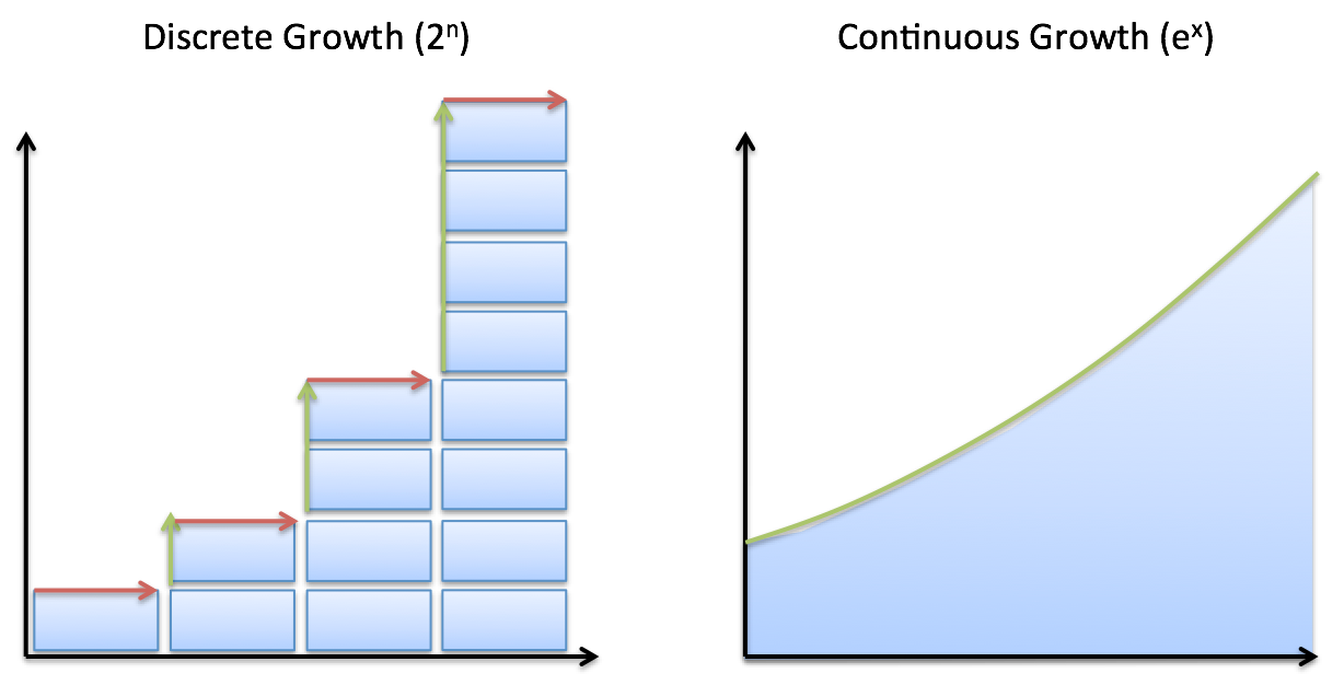\\n\",\n \"\\n\",\n \"## Demo \\n\",\n \"An ODENet approximated this spiral function better than a Recurrent Network. \\n\",\n \"\\n\",\n \"\\n\",\n \"\\n\",\n \"\\n\",\n \"## Why Does this matter? \\n\",\n \"\\n\",\n \"1. Faster testing time than recurrent networks, but slower training time. Perfect for low power edge computing! (precision vs speed)\\n\",\n \"2. More accurate results for time series predictions (!!) i.e continous-time models\\n\",\n \"3. Opens up a whole new realm of mathematics for optimizing neural networks (Diff Equation Solvers, 100+ years of theory)\\n\",\n \"4, Compute gradients with constant memory cost\\n\",\n \"\\n\",\n \"\\n\",\n \"## Concepts we'll learn about in this video\\n\",\n \"1. Basic neural network theory\\n\",\n \"2. \\\"Residual\\\" neural network theory\\n\",\n \"3. Ordinary Differential Equations (ODEs)\\n\",\n \"4. ODE Networks\\n\",\n \"5. Euler's Method to Optimize an ODENet\\n\",\n \"6. Adjoint Method for ODENet Optimization\\n\",\n \"7. ODENet's Applied to time series data\\n\",\n \"8. Future Applications of ODENets\\n\"\n ]\n },\n {\n \"metadata\": {\n \"id\": \"3wiokAO2RJyF\",\n \"colab_type\": \"text\"\n },\n \"cell_type\": \"markdown\",\n \"source\": [\n \"\\n\",\n \"\\n\",\n \"\\n\",\n \"\\n\"\n ]\n },\n {\n \"metadata\": {\n \"id\": \"qIlMUskCSA2Q\",\n \"colab_type\": \"text\"\n },\n \"cell_type\": \"markdown\",\n \"source\": [\n \"## 1 Basic Neural Network Theory\\n\",\n \"\\n\",\n \"- Neural Networks are a popular type of ML model\\n\",\n \"- Neural Networks are built with linear algebra (matrices & matrix operations) & optimized using Calculus (gradient descent & other algorithms)\\n\",\n \"- Neural networks consist of a series of \\\"layers\\\", which are just matrix operations\\n\",\n \"- Each layer introduces a little bit of error that compounds through the network\\n\",\n \"\\n\",\n \"#### Basic Neural Network Diagram \\n\",\n \"\\n\",\n \"\\n\",\n \"#### More Detailed Neural Network Diagram\\n\",\n \"\"\n ]\n },\n {\n \"metadata\": {\n \"id\": \"lheUH8Hh4qBN\",\n \"colab_type\": \"text\"\n },\n \"cell_type\": \"markdown\",\n \"source\": [\n \"## Basic Neural Network Example\"\n ]\n },\n {\n \"metadata\": {\n \"id\": \"bhKidD1YSDOM\",\n \"colab_type\": \"code\",\n \"outputId\": \"4e6b39f8-a51d-4591-f652-5dd29085f593\",\n \"colab\": {\n \"base_uri\": \"https://localhost:8080/\",\n \"height\": 106\n }\n },\n \"cell_type\": \"code\",\n \"source\": [\n \"import numpy as np\\n\",\n \"\\n\",\n \"# compute sigmoid nonlinearity\\n\",\n \"def sigmoid(x):\\n\",\n \" output = 1/(1+np.exp(-x))\\n\",\n \" return output\\n\",\n \"\\n\",\n \"# convert output of sigmoid function to its derivative\\n\",\n \"def sigmoid_output_to_derivative(output):\\n\",\n \" return output*(1-output)\\n\",\n \" \\n\",\n \"# input dataset\\n\",\n \"X = np.array([ [0,1],\\n\",\n \" [0,1],\\n\",\n \" [1,0],\\n\",\n \" [1,0] ])\\n\",\n \" \\n\",\n \"# output dataset \\n\",\n \"y = np.array([[0,0,1,1]]).T\\n\",\n \"\\n\",\n \"# seed random numbers to make calculation\\n\",\n \"# deterministic (just a good practice)\\n\",\n \"np.random.seed(1)\\n\",\n \"\\n\",\n \"# initialize weights randomly with mean 0\\n\",\n \"synapse_0 = 2*np.random.random((2,1)) - 1\\n\",\n \"\\n\",\n \"for iter in range(10000):\\n\",\n \"\\n\",\n \" # forward propagation\\n\",\n \" layer_0 = X\\n\",\n \" layer_1 = sigmoid(np.dot(layer_0,synapse_0))\\n\",\n \"\\n\",\n \" # how much did we miss?\\n\",\n \" layer_1_error = layer_1 - y\\n\",\n \"\\n\",\n \" # multiply how much we missed by the \\n\",\n \" # slope of the sigmoid at the values in l1\\n\",\n \" layer_1_delta = layer_1_error * sigmoid_output_to_derivative(layer_1)\\n\",\n \" synapse_0_derivative = np.dot(layer_0.T,layer_1_delta)\\n\",\n \"\\n\",\n \" # update weights\\n\",\n \" synapse_0 -= synapse_0_derivative\\n\",\n \"\\n\",\n \"print(\\\"Output After Training:\\\")\\n\",\n \"print(layer_1)\\n\"\n ],\n \"execution_count\": 0,\n \"outputs\": [\n {\n \"output_type\": \"stream\",\n \"text\": [\n \"Output After Training:\\n\",\n \"[[0.00505119]\\n\",\n \" [0.00505119]\\n\",\n \" [0.99494905]\\n\",\n \" [0.99494905]]\\n\"\n ],\n \"name\": \"stdout\"\n }\n ]\n },\n {\n \"metadata\": {\n \"id\": \"t8wkkYvbU32u\",\n \"colab_type\": \"text\"\n },\n \"cell_type\": \"markdown\",\n \"source\": [\n \"## Stack More Layers?\\n\",\n \"\\n\",\n \"- To reduce compounded error, add more layers! \\n\",\n \"\\n\",\n \"\\n\",\n \"\\n\",\n \"\\n\",\n \"\\n\",\n \"- The # of layers & # of neurons deeply affec the output of the network\\n\",\n \"- Too few layers could cause underfitting\\n\",\n \"- Too many layers coudl cause overfitting + long training time\\n\",\n \" \\n\",\n \" 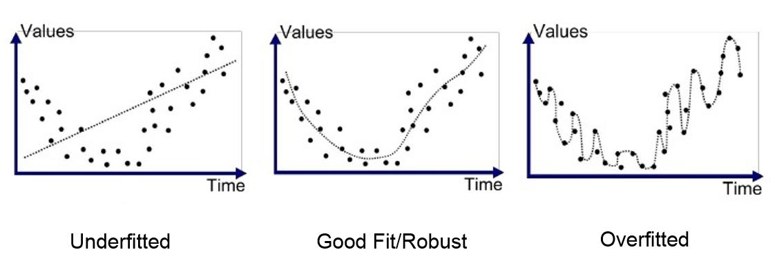\\n\",\n \"\\n\",\n \"#### There are many rule-of-thumb methods for determining the correct number of neurons to use in the hidden layers, such as the following:\\n\",\n \"\\n\",\n \"- The number of hidden neurons should be between the size of the input layer and the size of the output layer.\\n\",\n \"- The number of hidden neurons should be 2/3 the size of the input layer, plus the size of the output layer.\\n\",\n \"- The number of hidden neurons should be less than twice the size of the input layer\"\n ]\n },\n {\n \"metadata\": {\n \"id\": \"HASZaNUw7EKU\",\n \"colab_type\": \"text\"\n },\n \"cell_type\": \"markdown\",\n \"source\": [\n \"## Example: Long-Short Term Memory Neural Network with many layers\"\n ]\n },\n {\n \"metadata\": {\n \"id\": \"0bARtloGVdvF\",\n \"colab_type\": \"code\",\n \"colab\": {}\n },\n \"cell_type\": \"code\",\n \"source\": [\n \"\\n\",\n \"from keras.models import Sequential\\n\",\n \"from keras.layers import LSTM, Dense\\n\",\n \"import numpy as np\\n\",\n \"\\n\",\n \"data_dim = 16\\n\",\n \"timesteps = 8\\n\",\n \"num_classes = 10\\n\",\n \"\\n\",\n \"# expected input data shape: (batch_size, timesteps, data_dim)\\n\",\n \"model = Sequential()\\n\",\n \"model.add(LSTM(32, return_sequences=True,\\n\",\n \" input_shape=(timesteps, data_dim))) # returns a sequence of vectors of dimension 32\\n\",\n \"model.add(LSTM(32, return_sequences=True)) # returns a sequence of vectors of dimension 32\\n\",\n \"model.add(LSTM(32)) # return a single vector of dimension 32\\n\",\n \"\\n\",\n \"\\n\",\n \"\\n\",\n \"model.add(Dense(10, activation='softmax'))\\n\",\n \"\\n\",\n \"model.compile(loss='categorical_crossentropy',\\n\",\n \" optimizer='rmsprop',\\n\",\n \" metrics=['accuracy'])\\n\",\n \"\\n\",\n \"# Generate dummy training data\\n\",\n \"x_train = np.random.random((1000, timesteps, data_dim))\\n\",\n \"y_train = np.random.random((1000, num_classes))\\n\",\n \"\\n\",\n \"# Generate dummy validation data\\n\",\n \"x_val = np.random.random((100, timesteps, data_dim))\\n\",\n \"y_val = np.random.random((100, num_classes))\\n\",\n \"\\n\",\n \"model.fit(x_train, y_train,\\n\",\n \" batch_size=64, epochs=5,\\n\",\n \" validation_data=(x_val, y_val))\"\n ],\n \"execution_count\": 0,\n \"outputs\": []\n },\n {\n \"metadata\": {\n \"id\": \"Hfbs_m7PWrUm\",\n \"colab_type\": \"text\"\n },\n \"cell_type\": \"markdown\",\n \"source\": [\n \"## 2 Residual Neural Network Theory\\n\",\n \"\\n\",\n \"A solution to this was proposed by Microsoft for the 2015 ImageNet competiton (residual networks)\\n\",\n \"- In December of 2015, Microsoft proposed \\\"Residual networks\\\" as a solution to the ImageNet Classification Competition\\n\",\n \"- ResNets had the best accuracy in the competition\\n\",\n \"- ResNets utilize \\\"skip-connections\\\" between layers, which increases accuracy.\\n\",\n \"- They were able to train networks of up to 1000 layers deep while avoiding vanishing gradients (lower accuracy)\\n\",\n \"- 6 months later, their publicatio already had more than 200 references.\\n\",\n \"\\n\",\n \"\\n\",\n \"\\n\",\n \"\\n\",\n \"\\n\",\n \"\\n\",\n \"\\n\",\n \"\\n\",\n \"### How do ResNets work?\\n\",\n \"\\n\",\n \"- Instead of hoping each stack of layers directly fits a desired underlying mapping, we explicitly let these layers fit a residual mapping. \\n\",\n \"- The original mapping is recast into F(x)+x. \\n\",\n \"- Residual neural networks do this by utilizing skip connections or short-cuts to jump over some layers. \\n\",\n \"- The residual layer adds the output of the activation function to the input of the layer.\\n\",\n \"- This seemingly minor change has led to a rethinking of how neural network layers are designed.\\n\",\n \"- In its limit as ResNets it will only skip over a single layer\\n\",\n \"- With an additional weight matrix to learn the skip weights it is referred to as HighwayNets\\n\",\n \"- With several parallel skips it is referred to as DenseNets\\n\",\n \"\\n\",\n \"\\n\",\n \"The residual layer is actually quite simple: add the output of the activation function to the original input to the layer. As a formula, the k+1th layer has the formula:\\n\",\n \"\\n\",\n \"\\\\begin{equation} x_{k+1} = x_{k} + F(x_{k})\\\\end{equation}\\n\",\n \"\\n\",\n \"where F is the function of the kth layer and its activation. For example, F might represent a convolutional layer with a relu activation. This simple formula is a special case of the formula:\\n\",\n \"\\n\",\n \"\\\\begin{equation} x_{k+1} = x_{k} + h F(x_k),\\\\end{equation}\\n\",\n \"\\n\",\n \"which is the formula for the Euler method for solving ordinary differential equations (ODEs) when h=1\\n\",\n \"\\n\",\n \"### Wait, WTF is Euler's method? What does differential equations have to do with anything? Hold that thought, look at this code first.\\n\",\n \"\\n\"\n ]\n },\n {\n \"metadata\": {\n \"id\": \"auyfL0RBBa_C\",\n \"colab_type\": \"code\",\n \"colab\": {}\n },\n \"cell_type\": \"code\",\n \"source\": [\n \"#normal convolutional layer \\n\",\n \"\\n\",\n \"def Unit(x,filters):\\n\",\n \"\\n\",\n \" out = BatchNormalization()(x)\\n\",\n \" out = Activation(\\\"relu\\\")(out)\\n\",\n \" out = Conv2D(filters=filters, kernel_size=[3, 3], strides=[1, 1], padding=\\\"same\\\")(out)\\n\",\n \"\\n\",\n \" out = BatchNormalization()(out)\\n\",\n \" out = Activation(\\\"relu\\\")(out)\\n\",\n \" out = Conv2D(filters=filters, kernel_size=[3, 3], strides=[1, 1], padding=\\\"same\\\")(out)\\n\",\n \"\\n\",\n \" return out\"\n ],\n \"execution_count\": 0,\n \"outputs\": []\n },\n {\n \"metadata\": {\n \"id\": \"xUUXshvvBdim\",\n \"colab_type\": \"code\",\n \"colab\": {}\n },\n \"cell_type\": \"code\",\n \"source\": [\n \"#residual convolutional layer\\n\",\n \"\\n\",\n \"def Unit(x,filters):\\n\",\n \" res = x\\n\",\n \" out = BatchNormalization()(x)\\n\",\n \" out = Activation(\\\"relu\\\")(out)\\n\",\n \" out = Conv2D(filters=filters, kernel_size=[3, 3], strides=[1, 1], padding=\\\"same\\\")(out)\\n\",\n \"\\n\",\n \" out = BatchNormalization()(out)\\n\",\n \" out = Activation(\\\"relu\\\")(out)\\n\",\n \" out = Conv2D(filters=filters, kernel_size=[3, 3], strides=[1, 1], padding=\\\"same\\\")(out)\\n\",\n \"\\n\",\n \" out = keras.layers.add([res,out])\\n\",\n \"\\n\",\n \" return out\"\n ],\n \"execution_count\": 0,\n \"outputs\": []\n },\n {\n \"metadata\": {\n \"id\": \"jQqw9srmBQwA\",\n \"colab_type\": \"text\"\n },\n \"cell_type\": \"markdown\",\n \"source\": [\n \"\\n\",\n \"### Awesome, ok back to the question. What is the significance between residual networks and Ordinary Differential Equations? \\n\",\n \"\\n\",\n \"## 3 Ordinary Differential Equations\\n\",\n \"\\n\",\n \"- A \\\"differential equation\\\" is an equation that just tells us the slope without specifying the original function whose derivative we are taking\\n\",\n \"\\n\",\n \"\\n\",\n \"\\n\",\n \"\\n\",\n \"\\n\",\n \"\\n\",\n \"\\n\",\n \"\\n\",\n \"\\n\",\n \"\\n\",\n \"\\n\",\n \"\\n\"\n ]\n },\n {\n \"metadata\": {\n \"id\": \"aniJJUqACeKg\",\n \"colab_type\": \"text\"\n },\n \"cell_type\": \"markdown\",\n \"source\": [\n \"### Example Differential Equation \"\n ]\n },\n {\n \"metadata\": {\n \"id\": \"d1oTAMYFCYgF\",\n \"colab_type\": \"code\",\n \"outputId\": \"2e3038d1-8c41-40df-95ad-17ef18df37cf\",\n \"colab\": {\n \"base_uri\": \"https://localhost:8080/\",\n \"height\": 361\n }\n },\n \"cell_type\": \"code\",\n \"source\": [\n \"import numpy as np\\n\",\n \"from scipy.integrate import odeint\\n\",\n \"import matplotlib.pyplot as plt\\n\",\n \"\\n\",\n \"# function dy/dx = x + y/5.\\n\",\n \"func = lambda y,x : x + y/5.\\n\",\n \"# Initial condition\\n\",\n \"y0 = -3 # at x=0\\n\",\n \"# values at which to compute the solution (needs to start at x=0)\\n\",\n \"x = np.linspace(0, 4, 101)\\n\",\n \"# solution\\n\",\n \"y = odeint(func, y0, x)\\n\",\n \"# plot the solution, note that y is a column vector\\n\",\n \"plt.plot(x, y[:,0])\\n\",\n \"plt.xlabel('x')\\n\",\n \"plt.ylabel('y')\\n\",\n \"plt.show()\"\n ],\n \"execution_count\": 0,\n \"outputs\": [\n {\n \"output_type\": \"display_data\",\n \"data\": {\n \"image/png\": \"iVBORw0KGgoAAAANSUhEUgAAAe0AAAFYCAYAAAB+s6Q9AAAABHNCSVQICAgIfAhkiAAAAAlwSFlz\\nAAALEgAACxIB0t1+/AAAADl0RVh0U29mdHdhcmUAbWF0cGxvdGxpYiB2ZXJzaW9uIDIuMS4yLCBo\\ndHRwOi8vbWF0cGxvdGxpYi5vcmcvNQv5yAAAIABJREFUeJzt3Xl4lPW99/HPZCaZ7PskLGEL+you\\nFBRBQEBA3LAotp5qtWoPStunp+2x2h7bc57T69LHemxtLWrFKlrFgCIVD5ssLiCbsgSQELYsJJB9\\nzyQzcz9/oCkoJAGT+5578n5dF1dgJpn7++WX5DP39vs5DMMwBAAAgl6Y1QUAAID2IbQBALAJQhsA\\nAJsgtAEAsAlCGwAAmyC0AQCwCZfVBbSlpKSmQ18vKSlaFRX1HfqaVgmVXkKlD4leglWo9BIqfUj0\\n0hqPJ+68z3W5PW2Xy2l1CR0mVHoJlT4keglWodJLqPQh0cvF6nKhDQCAXRHaAADYBKENAIBNENoA\\nANgEoQ0AgE0Q2gAA2IQlod3Y2KipU6fqrbfesmLzAADYkiWh/Ze//EUJCQlWbBoAANsyPbQPHz6s\\n3NxcTZo0yexNAwBga6aH9uOPP66HH37Y7M0CAGB7ps49vnz5co0ePVq9evVq99ckJUV3+BRxrc3r\\najeh0kuo9CHRS7AKlV5CpQ8pNHrZtr9YPkeYupvUi6mhvXHjRuXn52vjxo0qLi5WRESEunXrpquu\\nuuq8X9PRE8p7PHEdvgiJVUKll1DpQ6KXYBUqvYRKH1Jo9PL58Qo98fpnmnFlX912TWaHvW5rb2ZM\\nDe2nn3665e/PPPOMevbs2WpgAwAQjAKGoTfWH5IkTR/b27Ttcp82AAAXaEt2sfJO1urK4eka2CvJ\\ntO1atp72ggULrNo0AAAXzdvk17JNhxXuCtOt1/Q3ddvsaQMAcAFWbctTZW2TrvtWbyXHR5q6bUIb\\nAIB2qqjx6n+3HldCTIRmjTPvXPaXCG0AANrprQ8Oq6k5oFsmZioywvwzzIQ2AADtcLy4Rpv3FivD\\nE6urR3a3pAZCGwCANhiGodfX5ciQNO/aAQoLc1hSB6ENAEAbdh4sUU5BlS4dmKphfZMtq4PQBgCg\\nFc0+v97ckCtnmEO3TR5gaS2ENgAArVizPV+lVY2aekWG0pOjLa2F0AYA4Dwqa716d8txxUWH64ar\\n+lldDqENAMD5vLXpiLxNft0yIVPRkZZNItqC0AYA4ByOFVfr471FyvDEauIlPawuRxKhDQDA1xiG\\nob+vPSRD0h0W3uL1VYQ2AABfsXX/SeUWVunyQR4NtfAWr68itAEAOIO3ya+sjYflcobptinW3uL1\\nVYQ2AABnWPnJcVXUeDVjbC95EqOsLucshDYAAF8oqWzQqq15Sopz6/pxfa0u52sIbQAAvvDm+lz5\\n/AHNndRf7gin1eV8DaENAICkA8fKtTOnRAN6JmjssHSryzknQhsA0OX5/AG9tu6QHJK+M22gHI7g\\nuMXrqwhtAECXt35ngU6U1mni6B7q2y3e6nLOi9AGAHRpVXVNeufjo4qJdGnOxEyry2kVoQ0A6NKW\\nbsxVg9evWyZmKi46wupyWkVoAwC6rMOFVfp4b7F6pcVq0uieVpfTJkIbANAlBQKGXl2bI0n67rRB\\nQTO/eGsIbQBAl/TBnhM6XlyjccPTNahXotXltAuhDQDocmobmrVs42FFRjg1d1JwzS/eGkIbANDl\\nLNt0WHWNPt10dT8lxbmtLqfdCG0AQJdy5ES1Pth1Qj1TY3Tt5RlWl3NBCG0AQJcRCBh6dc1BGZLu\\nnD5ILqe9YtBl5sYaGhr08MMPq6ysTF6vV/Pnz9fkyZPNLAEA0IV9sOeEjn1x8dng3klWl3PBTA3t\\nDRs2aMSIEbrvvvtUWFioe+65h9AGAJiipr6p5eKz2ybb5+KzM5ka2rNmzWr5e1FRkdLTg3MVFQBA\\n6Fm68fTFZ/OmDFBirH0uPjuTqaH9pXnz5qm4uFgLFy60YvMAgC4mt6BKH+4pUoYnVtdeYa+Lz87k\\nMAzDsGLDBw4c0C9+8QutWLGi1SXQfD6/XK7gW4gcAGAPfn9AP/mfTTpWVK3HH7paw/qlWF3SRTN1\\nTzs7O1spKSnq3r27hg4dKr/fr/LycqWknP8/sKKivkNr8HjiVFJS06GvaZVQ6SVU+pDoJViFSi+h\\n0odkbi9rtuXpWFG1JozqLk9sRIdvt6N78Xjizvucqde679ixQ4sWLZIklZaWqr6+XklJ9rt6DwBg\\nD+XVjXr7o9PLbn57Un+ry/nGTA3tefPmqby8XN/5znd0//336z/+4z8UFmave+QAAPbxxvpceZv8\\nmjt5QNAvu9keph4ej4yM1O9//3szNwkA6KKyj5Rpx+enNKBngq4e1d3qcjoEu7kAgJDT1OzX4jUH\\nFeZw6M7pgxTWygXPdkJoAwBCzj82H1NJZaOmj+ml3unnv7DLbghtAEBIKSyp1aqteUqJd+umq/tZ\\nXU6HIrQBACEjYBh6ZfVB+QOGvjttsNwRoTXPB6ENAAgZH+0p0qGCKl02yKPRA1OtLqfDEdoAgJBQ\\nXd+krA25ckc49Z2pA60up1MQ2gCAkLDk/VzVNfp0y4RMJcdHWl1OpyC0AQC2t+9oubbsK1bfbnGa\\nerl9FwRpC6ENALA1b7Nfr6z+XGEOh+6aMURhYaFxT/a5ENoAAFtb8fHR0/dkf6uX+nQLnXuyz4XQ\\nBgDYVt7JGq3emq/UhEjdND607sk+F0IbAGBLgYChl1d9roBh6HvXhd492edCaAMAbOn9nQU6WlSj\\nccPTNSIzxepyTEFoAwBsp7SyQcs+OKyYSJfmTQnNe7LPhdAGANiKYRh6efVBNTUHdMfUgYqPsf86\\n2e1FaAMAbGXLvmLtO1qu4f2SdeXwblaXYypCGwBgG9V1TXp93SG5w52667rBcoTIOtntRWgDAGzj\\n7+tyVNfo05yJmUpNjLK6HNMR2gAAW9iVW6ptB04ps0e8rg3hqUpbQ2gDAIJefWOzXln1uZxhDt09\\nM7SnKm0NoQ0ACHpvbshVZW2TbhjfVxmeWKvLsQyhDQAIavuOleuD3UXK8MRq1rg+VpdjKUIbABC0\\nGpt8evl/T6/gdc/1Q+Rydu3Y6trdAwCC2rJNR1Ra1aiZ43qrb7d4q8uxHKENAAhKOfmVen9ngbqn\\nROvG8X2tLicoENoAgKDjbfZr0XsH5JD0/VlDFe4K/RW82oPQBgAEnbc2HdGpigZNG9NLA3omWF1O\\n0CC0AQBBJSe/Uut25Cs9OVpzJmZaXU5QIbQBAEHjy8PiknTvrKGKCOew+JlcVmz0iSee0M6dO+Xz\\n+fTAAw9o+vTpVpQBAAgyyzYd1qmKBl33rV4akMFh8a8yPbQ/+eQTHTp0SEuWLFFFRYVuueUWQhsA\\ncPpq8R0F6pYcrVsmcFj8XEwP7TFjxmjUqFGSpPj4eDU0NMjv98vp5BAIAHRV3ia/Fq08fVj8nus5\\nLH4+pp/Tdjqdio6OliQtXbpUEydOJLABoIvL2pirU5UNum5sb64Wb4XDMAzDig2vW7dOzz33nBYt\\nWqS4uLjzfp7P55eL+/MAIGTtyjmlXz+3Rb3S4/T0/7mGvexWWHIh2ocffqiFCxfqr3/9a6uBLUkV\\nFfUdum2PJ04lJTUd+ppWCZVeQqUPiV6CVaj0Eip9SP/spb7Rp/95/VOFORz6/szBqqrs2N/5Zujo\\ncfF4zp+Lpod2TU2NnnjiCf3tb39TYmKi2ZsHAASRN94/pPJqr24c35e5xdvB9NB+7733VFFRoZ/8\\n5Cctjz3++OPq0aOH2aUAACy0K7dUH+0tUu/0WM2+qq/V5diC6aF9++236/bbbzd7swCAIFJV69Xf\\n/vdzuZwO/WD2sC6/5GZ78b8EADCVYRj689Ldqq5r0i0TM5XhibW6JNsgtAEAptqcXawte4s0qFei\\nrhvT2+pybIXQBgCYpqyqUX9fl6Mot0s/uH6owsIcVpdkK4Q2AMAUAcPQiyv3q8Hr1/03j1BqYpTV\\nJdkOoQ0AMMW67fn6PK9Slw5M1bUcFr8ohDYAoNMVnKrV0k1HFB8drrtmDJHDwWHxi0FoAwA6VbPP\\nr+f/sU8+f0B3zxqq+JgIq0uyLUIbANCplm06ooKSOk2+tKdGD0i1uhxbI7QBAJ1m37Fyrdmer27J\\n0bptygCry7E9QhsA0ClqG5r14rv75Qxz6P4bh8nN6l3fGKENAOhwhmHo5VWfq7K2STdP6MdiIB2E\\n0AYAdLgP9xRp58ESDcpI0MyxfawuJ2QQ2gCADlVUVtcy69l9Nwxn1rMORGgDADqMzx/Q8yv2q6k5\\noLtmDFZKQqTVJYUUQhsA0GHe+uCIjp+s0dWjuutbQ9OtLifkENoAgA6x71i5Vm3NU3pSlL4zdaDV\\n5YQkQhsA8I1V1zXpr//48vau4YqMcFldUkgitAEA38jp1bsOqKquSXMmZqpfd27v6iyENgDgG1m7\\nPV97j5RpRL9kXTeW1bs6E6ENALhox4qrtXTjYcXHROje2cMUxupdnYrQBgBclAavTwuX75M/YOi+\\n2cOUwOpdnY7QBgBcMMMwtHjNQZ2qbNDMcb01vF+y1SV1CYQ2AOCCfbSnSJ/sO6nMHvG6ZUKm1eV0\\nGYQ2AOCCFJbU6rW1OYp2u/TDG4fL5SRKzML/NACg3bxNfj27PFtNvoDuuX6oUhOjrC6pSyG0AQDt\\n9uragyoqq9fUyzN02SCP1eV0OYQ2AKBdPt5bpI/3FqtPtzjNnTzA6nK6JEIbANCmwtI6LV5zUFFu\\np/715hEKdxEfVuB/HQDQqsYmn559e6+amgP6/syhSuM8tmUsCe2cnBxNnTpVr776qhWbBwC0k2EY\\nemX1F+exr8jQFUPSrC6pSzM9tOvr6/Vf//VfuvLKK83eNADgAm3afaLlfuzbOI9tOdNDOyIiQi+8\\n8ILS0ni3BgDB7Hhxjf6+9pBiIl3615tGcD92EDB9BFwulyIjI83eLADgAtQ3NuvZ5Xvl8wd03w3D\\nlJLA7+1gEPSrlCclRcvlcnboa3o8cR36elYKlV5CpQ+JXoJVqPRiRh+BgKGFL21TSWWj5l47UNeO\\n69cp2wmVMZHM6yXoQ7uior5DX8/jiVNJSU2HvqZVQqWXUOlDopdgFSq9mNXHyi3HtG1/sYb2SdJ1\\nl2d0yjZDZUykju+ltTcAnKAAALTYf6xcb31wRElxbj1w03CFhbE+djAxfU87Oztbjz/+uAoLC+Vy\\nubR69Wo988wzSkxMNLsUAMAZyqsb9dyKfQpzODT/5hGKj2Z97GBjemiPGDFCixcvNnuzAIBW+PwB\\n/eWdbNXUN+u70wapf88Eq0vCOXB4HACg198/pMOF1Ro3PF1TLutpdTk4D0IbALq4j/YUacOnhcrw\\nxOquGUPkcHAeO1gR2gDQhR0tqtYrqw8q2u3SQ7eOlDu8Y2+xRccitAGgi6qub9Kf394rvz+g+28c\\nzkIgNkBoA0AX5A8E9Nw7+1Re7dXNE/ppVP8Uq0tCOxDaANAFZW04rAPHK3TpwFRdf1Vfq8tBOxHa\\nANDFbMku1prt+eqeEq0fzB6mMC48sw1CGwC6kGPF1frbqs8V5XZqwa2jFOUO+tmscQZCGwC6iOq6\\nJv3prb3y+QJ64Mbh6pYcbXVJuECENgB0AT5/QM++vVfl1V7NuSZTo/qnWl0SLgKhDQAhzjAM/X1t\\njnIKqnTFYI9mjetjdUm4SIQ2AIS49Z8WauOuE+qVFqt7rx/GjGc2RmgDQAg7cKxcr687pLjocC24\\ndaTcEcx4ZmeENgCEqFMV9Xp2ebYcDumhOSOVmsCMZ3ZHaANACGrw+vTHZXtV1+jT964brIEZiVaX\\nhA5AaANAiPEHAlr4zj6dKK3TtCt6acIlPawuCR2kzdD+4IMPzKgDANBBlqzP1d4jZRqRmazbpvS3\\nuhx0oDZDe/HixZo2bZr++Mc/qrCw0IyaAAAXaeNnhVq3o0A9UmP0wxtHyBnGAdVQ0ub8dS+88IKq\\nqqq0du1a/eY3v5EkzZkzR9OnT5fTyVWIABAs9h0r16trchQbFa4ff3uUoiOZojTUtOstWEJCgq6/\\n/nrNnj1bNTU1WrRokW666Sbt2rWrs+sDALRDUVmd/vJ2tsLCpAW3jpSHtbFDUptvw7Zv36633npL\\nW7du1bRp0/Tf//3f6t+/vwoKCvTQQw9p+fLlZtQJADiP6vomPZ21W/Ven+69fihXioewNkP7qaee\\n0rx58/Tb3/5WERERLY9nZGRo5syZnVocAKB1zT6//rRsr0oqG3XDVX01fmR3q0tCJ2oztF9//fXz\\nPvfAAw90aDEAgPYLGIZeXHlAuYVVGjssXTdP6Gd1SehkXFYIADa1/MMj2nbglAZkJOieWUOYU7wL\\nILQBwIY+3HNC724+rrTEKC2YM1LhLu7m6QoIbQCwmeyjZXpl1UHFRLr047mjFBcd0fYXISQQ2gBg\\nI3kna/Ts29lyOBxacOsodU+JsbokmIjQBgCbKKlo0NNZu9XY5Nd9NwzToF7c2tXVMF0OANhAfaNP\\n/++N7aqsbdJtkwdozJA0q0uCBUwP7d/97nfavXu3HA6HHnnkEY0aNcrsEgDAVpp9Af3prT06Xlyj\\nay/P0HXf6mV1SbCIqaG9bds2HT9+XEuWLNHhw4f1yCOPaMmSJWaWAAC2cvpe7P36PK9SV47srjuu\\nHcitXV2Yqee0t2zZoqlTp0qS+vfvr6qqKtXW1ppZAgDYypvrc1vuxf63716usDACuyszNbRLS0uV\\nlJTU8u/k5GSVlJSYWQIA2MaqrXlasz1f3VOi9aNbR8kdzr3YXZ2lF6IZhtHm5yQlRcvVwZMGeDxx\\nHfp6VgqVXkKlD4legpXdetn4aYHe3JCrlIRI/d9/Ha+0pGhJ9uujNfRy4UwN7bS0NJWWlrb8+9Sp\\nU/J4PK1+TUVFfYfW4PHEqaSkpkNf0yqh0kuo9CHRS7CyWy97j5Tpj0v3KMrt0o9vHSWHz6+Skhrb\\n9dEaemn99c7H1MPj48eP1+rVqyVJ+/btU1pammJjY80sAQCC2uHCKv357b0KC3Pox98epYw0fkfi\\nn0zd077ssss0fPhwzZs3Tw6HQ4899piZmweAoFZYWqens3bL5zP00JyRTJ6CrzH9nPbPfvYzszcJ\\nAEGvrKpRTy3ZpbpGn+6ZNVSjB6ZaXRKCENOYAoDFquua9OSSXaqo8Wru5P66elR3q0tCkCK0AcBC\\n9Y0+PfXmLp0sr9fMsb01c2wfq0tCECO0AcAi3ma//rB0t/JO1uqa0T307Un9rS4JQY7QBgAL+PwB\\n/fntvTpUUKVvDU3Tv0wfzPSkaBOhDQAmCwQMvfCP/co+Uq6RmSn6wexhTE+KdiG0AcBEAcPQS+8d\\n0PbPT2lQRoLm3zJCLie/itE+fKcAgEkMw9Bra3P0cXax+nWP04/nXsJ84rgghDYAmMAwDGVtPKwN\\nnxYqwxOr/3PbaEW5LV3+ATZEaAOACVZ8fEyrtuapW3K0fjZvtGKjwq0uCTZEaANAJ1u55Zje+eio\\nUhMi9fM7LlV8TITVJcGmCG0A6ESrtuZp2aYjSol36xd3XKqkOLfVJcHGCG0A6CTrduTrzQ25Sopz\\n6+d3XKrUxCirS4LNEdoA0Ak2fFaov687pISYCP38jkuVlhRtdUkIAYQ2AHSwjZ8VavHqg4qLDtfP\\n77hU3ZIJbHQMQhsAOtDGzwr1yhmB3SM1xuqSEEIIbQDoIF8N7AxPrNUlIcQQ2gDQAQhsmIHpeADg\\nG3p/Z4FeW5tDYKPTEdoA8A2s2ZanN9bnKv6Lq8R7cg4bnYjQBoCL9N4nx7V042Elxp4O7O4pBDY6\\nF6ENABdhxcdHtfzDo0qOPz1xSjr3YcMEhDYAXADDMLRs0xG998nxlrnEPcx0BpMQ2gDQTgHD0Ovr\\nDun9nQVKT4rSz++4VMnxkVaXhS6E0AaAdggEDP1t1ef6aE+Renpi9LPbRyshlsU/YC5CGwDa4PMH\\n9Nd392vbgVPq2y1OP72d9bBhDUIbAFrhbfbrL8uztedwmQZkJOgn375E0ZH86oQ1+M4DgPOob/Tp\\nj0t3K6egSiMyk/XgLSPlDndaXRa6MEIbAM6huq5JTy3ZpbxTtRozJE333TBMLiczP8NahDYAfEVp\\nVYN+v2S3TpbX65rRPfQv0wcrLMxhdVmA+QuGbNu2TVdeeaU2bNhg9qYBoE0Fp2r1u8U7dbK8XjPH\\n9db3riOwETxM3dPOy8vTSy+9pMsuu8zMzQJAu+TkV+qPS/eo3uvT7VMG6Lpv9ba6JOAspu5pezwe\\n/elPf1JcXJyZmwWANu06VKrfL9klb7Nf980eRmAjKJm6px0VxVR/AILPB7tP6JVVB+VyObTg1lEa\\n1T/F6pKAc+q00M7KylJWVtZZjy1YsEATJky4oNdJSoqWy9Wxt1h4PKGzpx8qvYRKHxK9BKtz9WIY\\nhv6++qDeWHtQcdER+o8fjNWQPskWVNd+oT4mdmVWL50W2nPnztXcuXO/8etUVNR3QDX/5PHEqaSk\\npkNf0yqh0kuo9CHRS7A6Vy8+f0CvrD6oj/YUKTUhUj+9fbRSosODuudQHxO76uheWnsDwC1fALqc\\nBq9PC9/Zp71HytSnW5x+MvcSJcREWF0W0CZTQ3vjxo168cUXdeTIEe3bt0+LFy/WokWLzCwBQBdX\\nUePVH7J2K+9UrUZkJmv+zSMUGcH+C+zB1O/USZMmadKkSWZuEgBa5J+q1dNZu1VR49U1o3vou9MG\\nMcsZbIW3lwC6hOwjZXp2ebYam/yaO6m/ZoztLYeDSVNgL4Q2gJD3v5uPauFbexUW5tAPbxqubw1N\\nt7ok4KIQ2gBCViBg6I31h7RuR4Fio8K14NaRGpiRaHVZwEUjtAGEpAavT8+t2Kc9h8vUKz1OD90y\\nQp5EJniCvRHaAEJOaWWD/rhsjwpK6jSiX7J+de841dc2Wl0W8I0R2gBCysG8Cv357WzVNjTr2ssy\\nNG/qAMVEhRPaCAmENoCQsXFXoV5bkyNJ+t51gzXp0p4WVwR0LEIbgO35/AEteT9X7396+oKzB28Z\\nocG9k6wuC+hwhDYAW6uua9JflmfrYH6lMjwxWnDrKC44Q8gitAHY1rHiav3prb0qr/bq8kEe3XP9\\nUEW5+bWG0MV3NwBb+nhvkV5edVB+f0C3TMzU7Cv7MMMZQh6hDcBWfP6AlqzP1fs7CxTldunBW0bo\\nkgGpVpcFmILQBmAbFTVePbt8rw4XVqtnaowenDNS3ZKjrS4LMA2hDcAWPj9eoYXvZKu6vlljh6Xr\\nrhmDWVITXQ7f8QCCWsAwtHprnpZtOiKHQ7pj6kBNvTyD89fokghtAEGrtqFZL767X7sPlykhNkLz\\nbx7Bgh/o0ghtAEHp8IkqLVyerbJqr4b1TdL9NwxXfEyE1WUBliK0AQQVwzC0dkeBsjbkKhAwdNPV\\n/XTDVX0VFsbhcIDQBhA0zjwcHhcdrvtvHK7hfZOtLgsIGoQ2gKCQk1+p51bsU0WNV0P7JOm+G4Yp\\nMdZtdVlAUCG0AVjKHwho5ebjeufjo3LIoTkTMzVrXB8OhwPnQGgDsExpVYOe/8d+5RZUKTnerftv\\nGK5Bvbg6HDgfQhuAJbbuP6lXVh9Ug9enK4ak6a4ZgxUTGW51WUBQI7QBmKq+0ae/r8vR5uxiucOd\\n+v6sIbp6ZHcmSwHagdAGYJqDeRX667v7VVbtVd9ucXrgxuFKZ+5woN0IbQCdrtkX0NsfHNHqbXly\\nOBy6cXxfzb6qr1zOMKtLA2yF0AbQqY4X1+ivK/ersKROaUlRum/2MPXvmWB1WYAtEdoAOoXPH9C7\\nm4/p3c3HFTAMTbq0p26b3J+VuYBvgJ8eAB2u4FSt/rpyv/JO1io53q3vzxyq4f2Y2Qz4pkwNbZ/P\\np0cffVR5eXny+/36xS9+oSuuuMLMEgB0Ip8/oJVbjuvdzcfkDxi6elR3zZsyUNGR7B8AHcHUn6R3\\n3nlHUVFRev3113Xo0CH98pe/1NKlS80sAUAnOVpUrZfeO6CCkjolxbl114zBGtU/1eqygJBiamjf\\neOONmj17tiQpOTlZlZWVZm4eQCfwNvu14qOjWrUtT4YhXTO6h+ZOGsDeNdAJTP2pCg//52xHL7/8\\nckuAA7CnfUfL9crqz1VS2ajUhEjdPXOIhrEqF9BpHIZhGJ3xwllZWcrKyjrrsQULFmjChAl67bXX\\ntH79ei1cuPCsID8Xn88vl8vZGSUCuEhVtV69uCJbG3YWKMwh3XTNAH1n+mBFutm7BjpTp4X2+WRl\\nZWnVqlV69tln5Xa3vexeSUlNh27f44nr8Ne0Sqj0Eip9SKHfS8Aw9PGeImVtPKzahmb1SY/T3TOH\\nqE+3OIuqbJ9QGZdQ6UOil7Ze73xMfVucn5+vN954Q6+++mq7AhtA8CgoqdXi1Qd1qKBK7nCnbp8y\\nQFOvyJAzjFnNALOYGtpZWVmqrKzU/fff3/LYiy++qIiICDPLAHABGrw+/WPzMa3dni9/wNDlgzy6\\nY+pAJcdHWl0a0OWYGto//elP9dOf/tTMTQK4SIZh6JP9xXpzfa4qa5uUmhCp704bpEsGcBsXYBWu\\nGgHwNQUltfqfrD3ae7hULmeYbhzfVzPH9ZE7nItCASsR2gBa1DY0a/mHR7TxsxMKGIZGD0jVvGsH\\nKC2J5TOBYEBoA5DPH9CGzwq14qOjqmv0KT0pSg/MGaW+nhirSwNwBkIb6MIMw9Cew2V6c0Ouisrq\\nFeV26fYpA3Tt5Rnq3i0hZG7JAUIFoQ10UXkna7Rkfa4OHK+QwyFNGt1DN0/MVHw0d3MAwYrQBrqY\\nsqpGLf/wiDZnF8uQNDIzRXMn91eGJ9bq0gC0gdAGuojahmat3HJM7+8slM8fUIYnVrdPGcA614CN\\nENpAiPM2+bVuZ77e++S4Grx+pcS7dfOETF05vJvCwhxWlwfgAhDaQIhq9vm18bMTWrnlmKrrmxUb\\nFa55U/pp8mU9Fc4iPIAtEdpAiPH5A/pob5H+8fExVdR4FRnh1I3j+2r6mN6scQ3YHD/BQIj4MqxX\\nbj6msmqvIlxhmjm2t2aM7a04rggHQgKhDdhcsy+gj/cWaeWW02Ed7grTtCt6aea43kqMZTU9IJQQ\\n2oBNeZv82rT7hFZvy1NFDWH1var8AAAOr0lEQVQNdAWENmAz9Y3NWv9podZsz1dtQ7Pc4U5NH9NL\\nM8YS1kCoI7QBmyivbtSa7fnatPuEvE1+RbtdunF8X029opdio8KtLg+ACQhtIMjlnazRmu352rr/\\npPwBQ4mxEbpxfF9NGt1TUW5+hIGuhJ94IAgFvljIY+32fB04XiFJ6p4SrZlj+2jc8HS5nGEWVwjA\\nCoQ2EEQavD5tzi7Wup0FOlleL0ka2idJ08b00qj+KQpzMIMZ0JUR2kAQKCqr0/qdhfoou0jeJr9c\\nTofGj+ymaVf0Uu/0OKvLAxAkCG3AIj5/QJ8dKtXGzwpbDoEnxbk1a1wfTbykhxJimBAFwNkIbcBk\\nJZUN+mD3CX24p0jVdU2SpMG9EnXt5RkaPTCV89UAzovQBkzQ7PNrZ06JPtxd1LJXHe12adoVvXTN\\n6B7qkRpjcYUA7IDQBjqJYRg6WlSjzdlF2rr/pOoafZKkQRkJmnBJD40ZkqaIcFbbAtB+hDbQwcqq\\nGvXJ/mJtzi5WUdnpK8DjYyI0c1xvTRjVQ92Soy2uEIBdEdpAB6ipb9KOgyX69FCp9h0pkyS5nGEa\\nMyRN40d20/B+yXKGca4awDdDaAMXqa6xWZ/mlGjH5yXaf6xc/oAhh0Ma0jtRY4ela8yQNEVHMr0o\\ngI5DaAMXoKa+SbtyS7XzYIn2HT0d1JLUJz1OY4ela+bVmTKafRZXCSBUEdpAG0qrGvTZoVJ9llOi\\ng/mVMk7ntHqnx2rMkDRdMSRN6Umnz1OnJkappKTGwmoBhDJCG/iKQMDQkaJq7c4t1e7cUhWU1LU8\\n179nvC4b5NFlgzwtQQ0AZjE1tMvKyvTv//7v8nq9am5u1i9/+UtdcsklZpYAnFNVXZP2HS1T9pFy\\nZR8tV21Ds6TTF5ONzEzR6AEpGj3Qo6Q41qsGYB1TQ3vFihW66aabdMMNN2jbtm36wx/+oEWLFplZ\\nAiBJ8jb7daigUvuPVWj/sXLlnaxteS4pzq0Jo7pr9IBUDeubLHcE91IDCA6mhvb3v//9lr8XFRUp\\nPT3dzM0rYBhq9vlN3SaCQ1OzX4dPVOtgXoVy8iuVW1gln//0yWmX06GhfZI0MjNFIzKT1TM1Rg5W\\n0wIQhEw/p11SUqIf/vCHqqur08svv2zqtv9nyS59nlepjLRY9e8Rr/49EtSvR7zSkqJY8jDE1DY0\\nK7egSocKK5VbUKWjRdUtIe2Q1Cs9VsP6JmtY3yQNzEiUm5nJANiAwzC+vBa2Y2VlZSkrK+usxxYs\\nWKAJEyZIkjZt2qSXX365zcPjPp9fLlfH/EJdty1Pqz45psMFVfL5Ay2Px0S61D8jUQN7JWpAr0Rl\\n9kxQt+QYhYUR5Hbg8wd07Mu96C/+FJz65+HuMIfUr2eCRmSmamT/FA3PTFFsNCtoAbCfTgvtc9m2\\nbZsGDx6shIQESdLYsWO1devWVr+mo2+f8XjidKKoSnmnanS4sFrHiqp1tLhGJ8vrz/q8KLdTvdLi\\n1DstVhlpscrwxKpnakxQnd/0eOJC4vaiC+mj2efXidJ6HT9Zo2PFNTpeXKOCklo1+/75Jswd4VT/\\nHvEa0DNBAzMSldkjXlFucw4qhcqYSPQSjEKlD4le2nq98zH18PiaNWu0f/9+3X333Tp48KC6d+9u\\n5uZbhLvC1L9Hgvr3SGh5rL6xWceKa5R3slZ5J2t0/GSNDhVUKie/suVzHJI8SVHqkRKjHqkx6pEa\\nre4pMeqWHG1aKHQVgYChkqoGnSit04nSOuWfqlVBSZ2Ky+oVOON9pjPMoZ6eGPXrHq/M7vHK7BGv\\n7ikcJQEQmkxNmvnz5+vhhx/W2rVr1dTUpN/85jdmbr5V0ZHhX5zjTG55zNvkV0FprQpL6lRwqlYF\\nJaeDY1duqXbllp719QmxEeqWFK305GilJUUpLTFKnsQopSVFEejnYRiGahqaVXa8XAePlKq4vEHF\\n5fUqLqtXcXn9WacwJCkywqnMnvHq5YlVn25x6pMepx6pMQp3Mac3gK7B1DRJTk7W888/b+Ymv5HT\\nh1nP3iOXpOr6JhWV1ulEWb1OlNbpZPnpkMnJr9TBM/bMvxTtdik1IVIpCZFKiY9UcnykkuLcLX8S\\nYyMU3kHn7YOJzx9QVW2TKmq9Kq9uVHm1V2XVjSqvblRJZYNKqhrlbfr61fwR4WHq6Yn54ohGtHqk\\nxCgjLVYpCZFcMAigS2MX8CLER0covneEBvdOOuvxZp9fpyoadKqyQSVffDxV2aCyqkYVV9Qr74yL\\no74qyu1SYmyEEmIiFBsdobiocMVFhys2KlwxUeGKdrsUExmu6EiXotwuRUY4FQiYdjmCfP6AGrw+\\nNTT51dDoU31js+oafaprbFZtQ7Nq6ptVXd+kmromVdU1q6rOq5r65vO+njvCKU9ClDyJkerTI0Hx\\nkS6lJ0crPSlKiXFuwhkAzoHQ7kDhLqd6emLV0xP7tedaDgVXNaqyxqvyGq8qaryqqGlUdV2Tquqa\\nVFnb1LL+cnu5w51yh4cpItypcNcXH51hcoY55HI65HSGKczhkMOhlo+GJMM4XZNhSP6AIZ8/IL8/\\nIH/AULMvIK8voKZmv5qa/fI2+1tul2qPyAinEmPd6pkao8RYtxJj3UqKdysl/ssjDW7FRoW33Asd\\nShekAEBnIrRN4nA4Tu+hR0dIrVx/5/MHVNfQrJov9l5r6ptU/8Ue7emPPjU2+dTY5JffkGrqvGpq\\nDqjJ51dNfbOafd7TAXyRe+Eup0MuZ5jcX7wJSIx1KyLcqSi3U1ERLkV+8TEmKlwxkV9+DFd8TLji\\noiIUFx2uCO55BoBOQWgHGZczTAmxbiXEtj3HdWt7qIZhtOxBBwKSodN71YEv1nx2OBw6fYG1Q84w\\nh5zO0x+ZCQwAghehHaIcDkfLXjMAIDTwGx0AAJsgtAEAsAlCGwAAmyC0AQCwCUIbAACbILQBALAJ\\nQhsAAJsgtAEAsAlCGwAAmyC0AQCwCUIbAACbcBiGYd6izAAA4KKxpw0AgE0Q2gAA2AShDQCATRDa\\nAADYBKENAIBNENoAANiEy+oCOsvvfvc77d69Ww6HQ4888ohGjRrV8tzmzZv11FNPyel0auLEiXrw\\nwQctrLRtrfUyZcoUdevWTU6nU5L05JNPKj093apS25STk6P58+fr7rvv1p133nnWc3Ybl9Z6sdO4\\nPPHEE9q5c6d8Pp8eeOABTZ8+veU5u41Ja73YaUwaGhr08MMPq6ysTF6vV/Pnz9fkyZNbnrfLuLTV\\nh53G5EuNjY2aPXu25s+frzlz5rQ8btqYGCFo69atxv33328YhmHk5uYat91221nPz5w50zhx4oTh\\n9/uNO+64wzh06JAVZbZLW71MnjzZqK2ttaK0C1ZXV2fceeedxq9+9Stj8eLFX3veTuPSVi92GZct\\nW7YYP/jBDwzDMIzy8nLjmmuuOet5O41JW73YZUwMwzBWrlxpPP/884ZhGEZBQYExffr0s563y7i0\\n1YedxuRLTz31lDFnzhxj2bJlZz1u1piE5OHxLVu2aOrUqZKk/v37q6qqSrW1tZKk/Px8JSQkqHv3\\n7goLC9M111yjLVu2WFluq1rrxW4iIiL0wgsvKC0t7WvP2W1cWuvFTsaMGaM//OEPkqT4+Hg1NDTI\\n7/dLst+YtNaL3cyaNUv33XefJKmoqOisvU87jUtrfdjR4cOHlZubq0mTJp31uJljEpKHx0tLSzV8\\n+PCWfycnJ6ukpESxsbEqKSlRcnLyWc/l5+dbUWa7tNbLlx577DEVFhbq8ssv17/927/J4XBYUWqb\\nXC6XXK5zf8vZbVxa6+VLdhgXp9Op6OhoSdLSpUs1ceLElkOVdhuT1nr5kh3G5Ezz5s1TcXGxFi5c\\n2PKY3cZFOncfX7LTmDz++OP69a9/reXLl5/1uJljEpKh/VVGCM3U+tVefvSjH2nChAlKSEjQgw8+\\nqNWrV2vGjBkWVYcv2W1c1q1bp6VLl2rRokVWl/KNna8Xu42JJL3xxhs6cOCAfv7zn2vFihVBHWit\\nOV8fdhqT5cuXa/To0erVq5eldYTk4fG0tDSVlpa2/PvUqVPyeDznfO7kyZNBfYiztV4k6eabb1ZK\\nSopcLpcmTpyonJwcK8r8xuw2Lm2x07h8+OGHWrhwoV544QXFxcW1PG7HMTlfL5K9xiQ7O1tFRUWS\\npKFDh8rv96u8vFySvcaltT4ke43Jxo0b9f777+u2225TVlaWnn32WW3evFmSuWMSkqE9fvx4rV69\\nWpK0b98+paWltRxOzsjIUG1trQoKCuTz+bRhwwaNHz/eynJb1VovNTU1uvfee9XU1CRJ2r59uwYO\\nHGhZrd+E3calNXYal5qaGj3xxBN67rnnlJiYeNZzdhuT1nqx05hI0o4dO1qOFJSWlqq+vl5JSUmS\\n7DUurfVhtzF5+umntWzZMr355puaO3eu5s+fr6uuukqSuWMSsqt8Pfnkk9qxY4ccDocee+wx7d+/\\nX3FxcZo2bZq2b9+uJ598UpI0ffp03XvvvRZX27rWenn55Ze1fPlyud1uDRs2TL/+9a+D9hBadna2\\nHn/8cRUWFsrlcik9PV1TpkxRRkaG7calrV7sMi5LlizRM888o379+rU8NnbsWA0ePNh2Y9JWL3YZ\\nE+n0bUWPPvqoioqK1NjYqIceekiVlZW2+x3WVh92GpMzPfPMM+rZs6ckmT4mIRvaAACEmpA8PA4A\\nQCgitAEAsAlCGwAAmyC0AQCwCUIbAACbILQBALAJQhsAAJsgtAG0eOmll/SrX/1KknTkyBHNmDHD\\ntqvKAaGI0AbQ4q677tLRo0e1c+dO/fa3v9V//ud/nrWiHABrMSMagLMcP35cd955p2bMmKFHH33U\\n6nIAnIE9bQBnqaqqUnR0dMvqTACCB6ENoIXX69Vjjz2mhQsXKjw8XMuXL7e6JABn4PA4gBZPPPGE\\nYmJi9OCDD6q0tFS33367XnvtNXXr1s3q0gCI0AYAwDY4PA4AgE0Q2gAA2AShDQCATRDaAADYBKEN\\nAIBNENoAANgEoQ0AgE0Q2gAA2MT/BxLE0LUjCQqWAAAAAElFTkSuQmCC\\n\",\n \"text/plain\": [\n \"\"\n ]\n },\n \"metadata\": {\n \"tags\": []\n }\n }\n ]\n },\n {\n \"metadata\": {\n \"id\": \"Z2DbYdsRCdDq\",\n \"colab_type\": \"text\"\n },\n \"cell_type\": \"markdown\",\n \"source\": [\n \"## 4 ODE (Ordinary Differential Equation) Networks\\n\",\n \"\\n\",\n \"\\n\",\n \"Consider a simplified ODE from physics: we want to model the position x of a marble. Assume we can calculate its velocity x′ (the derivative of position) at any position x. We know that the marble starts at rest x(0)=0 and that its velocity at time t depends on its position through the formula:\\n\",\n \"\\n\",\n \"\\\\begin{equation} x^\\\\prime(t) = f(x) \\\\end{equation}\\n\",\n \"\\n\",\n \"The Euler method solves this problem by following the physical intuition: my position at a time very close to the present depends on my current velocity and position. For example, if you are travelling at a velocity of 5 meters per second, and you travel 1 second, your position changes by 5 meters. If we travel h seconds, we will have travelled 5h meters. As a formula, we said:\\n\",\n \"\\n\",\n \"\\\\begin{equation}x(t+h) = x(t) + h x^\\\\prime(t),\\\\end{equation}\\n\",\n \"\\n\",\n \"but since we know\\n\",\n \"\\n\",\n \"\\\\begin{equation} x^\\\\prime(t) = f(x) \\\\end{equation}\\n\",\n \"\\n\",\n \"we can rewrite this as\\n\",\n \"\\n\",\n \"\\\\begin{equation} x(t+h) = x(t) + h f(x).\\\\end{equation}\\n\",\n \"\\n\",\n \"If you squint at this formula for the Euler method, you can see it looks just like the formula for residual layers!\\n\",\n \"\\n\",\n \"This observation has meant three things for designing neural networks:\\n\",\n \"\\n\",\n \"- New neural network layers can be created through different numerical approaches to solving ODEs\\n\",\n \"- The possibility of arbitrarily deep neural networks\\n\",\n \"- Training of a deep network can be improved by considering the so-called stability of the underlying ODE and its numerical discretization\\n\",\n \"\\n\",\n \"### 2 more points\\n\",\n \"\\n\",\n \"- To create arbitrarily deep networks with a finite memory footprint, design neural networks based on stable ODEs and numerical discretizations.\\n\",\n \"- Gradient descent can be viewed as applying Euler's method for solving ordinary differential equation to gradient flow. \\n\",\n \"\\n\",\n \"\\n\"\n ]\n },\n {\n \"metadata\": {\n \"id\": \"AqolUsWEnrh1\",\n \"colab_type\": \"text\"\n },\n \"cell_type\": \"markdown\",\n \"source\": [\n \"\\n\",\n \"\\n\",\n \"## What Does an ODENet Look like? \\n\",\n \"\\n\",\n \"*An ODE is a function that usually describes the change of some system through time. In this setting, time is a continuous variable. Now imagine a neural network is that system, and time is really something more like the depth of the network. Note that there are usually a discrete number of layers in an ANN. This is a notion of continuous number of layers.*\\n\",\n \"\\n\",\n \"- The team didn't use Euler's method, they computed the exact ODE solution (within a small error tolerance) using adaptive solvers (faster)\\n\",\n \"- The dynamics change smoothly with depth. You can think of this either as having weights that are a function of depth, or as having shared weights across layers but adding the depth as an extra input to f.\\n\",\n \"- Anywhere you can put a resnet you can put an ODEnet.\\n\",\n \"- Each ODEBlock can be used to replace a whole stack of ResBlocks.\\n\",\n \"- In their MNIST example, each ODEBlock replaces 6 ResBlocks.\\n\",\n \"\\n\",\n \"### Traditional Deep Nets\\n\",\n \"\\n\",\n \"\\n\",\n \"```\\n\",\n \"h1 = f1(x)\\n\",\n \"h2 = f2(h1)\\n\",\n \"h3 = f3(h2)\\n\",\n \"h4 = f3(h3)\\n\",\n \"y = f5(h4)\\n\",\n \"```\\n\",\n \"\\n\",\n \"### ResNets\\n\",\n \"\\n\",\n \"```\\n\",\n \"h1 = f1(x) + x\\n\",\n \"h2 = f2(h1) + h1\\n\",\n \"h3 = f3(h2) + h2\\n\",\n \"h4 = f4(h3) + h3\\n\",\n \"y = f5(h4) + h4\\n\",\n \"```\\n\",\n \"\\n\",\n \"\\n\",\n \"- Where f1, f2, etc are neural net layers.\\n\",\n \"- The idea is that it's easier to model a small change to an almost-correct answer than to output the whole improved answer at once.\\n\",\n \"-This looks like a primitive ODE solver (Euler's method) that solves the trajectory of a system by just taking small steps in the direction of the system dynamics and adding them up.\\n\",\n \"-They connection allows for better training methods.\\n\",\n \"- What if we define a deep net as a continuously evolving system? \\n\",\n \"- Instead of updating the hidden units layer by layer, we define their derivative with respect to depth instead\\n\",\n \"- We can use off-the-shelf adaptive ODE solvers to compute the final state of these dynamics, and call that the output of the neural network. \\n\",\n \"\\n\",\n \"## 5 Euler's Method \\n\",\n \"\\n\",\n \"\\n\",\n \"\\n\",\n \"\\n\",\n \"- We want to recover the blue curve, but all we have is an initial point A_0 (think inputs to the network) and a differential equation.\\n\",\n \"- From the differential equation, we can calculate the tangent line. If we take a small step along the tangent line, we arrive at A_1, which will be close to the desired blue line if the step is small enough. \\n\",\n \"- Repeat this process to uncover a polygonal curve A_{0}A_{1}A_{2}...A_{n}.\\n\",\n \"\\n\",\n \"Many neural networks have a composition that looks exactly like the steps of Euler’s method. We start with an initial state \\\\mathbf{z}_0, and apply successive transformations over time (layers):\\n\",\n \"\\n\",\n \"\\n\",\n \"\\n\",\n \"\\n\",\n \"\\n\",\n \"\\n\",\n \"\\n\",\n \"…\\n\",\n \"\\n\",\n \"\\n\",\n \"\\n\",\n \"\\n\",\n \"### In the limit, we parameterize the continuous dynamics of hidden units using an ordinary differential equation (ODE) specified by a neural network:\\n\",\n \"\\n\",\n \"\\n\",\n \"\\n\",\n \"### The equivalent of having T layers in the network, is finding the solution to this ODE at time T.\\n\",\n \"\\n\",\n \"\\n\",\n \"\\n\",\n \"- Euler’s method is perhaps the simplest method for solving ODEs. \\n\",\n \"- There since been more than 120 years of development of efficient and accurate ODE solvers. \\n\",\n \"- Modern ODE solvers provide guarantees about the growth of approximation error, monitor the level of error, and adapt their evaluation strategy on the fly to achieve the requested level of accuracy. \\n\",\n \"- This allows the cost of evaluating a model to scale with problem complexity.\\n\",\n \"\\n\",\n \"\\n\",\n \"### We’ve seen how to feed-forward, but how do you efficiently train a network defined as a differential equation? The answer lies in the adjoint method (which dates back to 1962). Think of the adjoint as the instantaneous analog of the chain rule.\\n\",\n \"\\n\",\n \"## 6 The Adjoint Method\\n\",\n \"\\n\",\n \"- This approach computes gradients by solving a second, augmented ODE backwards in time, and is applicable to all ODE solvers. \\n\",\n \"- This approach scales linearly with problem size, has low memory cost, and explicitly controls numerical error.\\n\",\n \"- The adjoint captures how the loss function L changes with respect to the hidden state.\\n\",\n \"- Starting from the output of the network, we can recompute the hidden state backwards in time together with the adjoint.\\n\",\n \"\\n\",\n \"\\n\",\n \"\\n\",\n \"\\n\",\n \"- A third integral then tells us how the loss changes with the parameters \\\\theta ( dL/d\\\\theta).\\n\",\n \"- All three of these integrals can be computed in a single call to an ODE solver, which concatenates the original state, the adjoint, and the other partial derivatives into a single vector. \\n\",\n \"- Algorithm 1 shows how to construct the necessary dynamics, and call an ODE solver to compute all gradients at once.\\n\",\n \"\\n\",\n \"\\n\",\n \"\\n\",\n \"\\n\"\n ]\n },\n {\n \"metadata\": {\n \"id\": \"BV2evfTpMCo-\",\n \"colab_type\": \"text\"\n },\n \"cell_type\": \"markdown\",\n \"source\": [\n \"## ODE Net Example\"\n ]\n },\n {\n \"metadata\": {\n \"id\": \"Jx1aVJHqqRLv\",\n \"colab_type\": \"code\",\n \"outputId\": \"2cd9a555-cf13-4a48-e59c-939c8c837dc3\",\n \"colab\": {\n \"base_uri\": \"https://localhost:8080/\",\n \"height\": 317\n }\n },\n \"cell_type\": \"code\",\n \"source\": [\n \"## Import the Adjoint Method (ODE Solver)\\n\",\n \"from torchdiffeq import odeint_adjoint as odeint\\n\",\n \"\\n\",\n \"## Normal Residual Block Example\\n\",\n \"\\n\",\n \"class ResBlock(nn.Module):\\n\",\n \"\\n\",\n \" #init a block - Convolve, pool, activate, repeat\\n\",\n \" def __init__(self, inplanes, planes, stride=1, downsample=None):\\n\",\n \" super(ResBlock, self).__init__()\\n\",\n \" self.norm1 = norm(inplanes)\\n\",\n \" self.relu = nn.ReLU(inplace=True)\\n\",\n \" self.downsample = downsample\\n\",\n \" self.conv1 = conv3x3(inplanes, planes, stride)\\n\",\n \" self.norm2 = norm(planes)\\n\",\n \" self.conv2 = conv3x3(planes, planes)\\n\",\n \"\\n\",\n \" #Forward pass - pass output of one layer to the input of the next \\n\",\n \" def forward(self, x):\\n\",\n \" shortcut = x\\n\",\n \" out = self.relu(self.norm1(x))\\n\",\n \" out = self.conv1(out)\\n\",\n \" out = self.norm2(out)\\n\",\n \" out = self.relu(out)\\n\",\n \" out = self.conv2(out)\\n\",\n \"\\n\",\n \" return out + shortcut\\n\",\n \"\\n\",\n \"## Ordinary Differential Equation Definition \\n\",\n \"\\n\",\n \"class ODEfunc(nn.Module):\\n\",\n \"\\n\",\n \" # init ODE variables\\n\",\n \" def __init__(self, dim):\\n\",\n \" super(ODEfunc, self).__init__()\\n\",\n \" self.norm1 = norm(dim)\\n\",\n \" self.relu = nn.ReLU(inplace=True)\\n\",\n \" self.conv1 = conv3x3(dim, dim)\\n\",\n \" self.norm2 = norm(dim)\\n\",\n \" self.conv2 = conv3x3(dim, dim)\\n\",\n \" self.norm3 = norm(dim)\\n\",\n \" self.nfe = 0\\n\",\n \"\\n\",\n \" # init ODE operations \\n\",\n \" def forward(self, t, x):\\n\",\n \" #nfe = number of function evaluations per timestep\\n\",\n \" self.nfe += 1\\n\",\n \" out = self.norm1(x)\\n\",\n \" out = self.relu(out)\\n\",\n \" out = self.conv1(out)\\n\",\n \" out = self.norm2(out)\\n\",\n \" out = self.relu(out)\\n\",\n \" out = self.conv2(out)\\n\",\n \" out = self.norm3(out)\\n\",\n \" return out\\n\",\n \"\\n\",\n \"\\n\",\n \" ## ODE block\\n\",\n \"class ODEBlock(nn.Module):\\n\",\n \"\\n\",\n \" #initialized as an ODE Function\\n\",\n \" #count the time\\n\",\n \" def __init__(self, odefunc):\\n\",\n \" super(ODEBlock, self).__init__()\\n\",\n \" self.odefunc = odefunc\\n\",\n \" self.integration_time = torch.tensor([0, 1]).float()\\n\",\n \"\\n\",\n \" #foorward pass \\n\",\n \" #input the ODE function and input data into the ODE Solver (adjoint method)\\n\",\n \" # to compute a forward pass\\n\",\n \" def forward(self, x):\\n\",\n \" self.integration_time = self.integration_time.type_as(x)\\n\",\n \" out = odeint(self.odefunc, x, self.integration_time, rtol=args.tol, atol=args.tol)\\n\",\n \" return out[1]\\n\",\n \"\\n\",\n \" @property\\n\",\n \" def nfe(self):\\n\",\n \" return self.odefunc.nfe\\n\",\n \"\\n\",\n \" @nfe.setter\\n\",\n \" def nfe(self, value):\\n\",\n \" self.odefunc.nfe = value\\n\",\n \"\\n\",\n \"## Main Method\\n\",\n \"\\n\",\n \"if __name__ == '__main__':\\n\",\n \"\\n\",\n \"\\n\",\n \" \\n\",\n \" #Add Pooling\\n\",\n \" downsampling_layers = [\\n\",\n \" nn.Conv2d(1, 64, 3, 1),\\n\",\n \" ResBlock(64, 64, stride=2, downsample=conv1x1(64, 64, 2)),\\n\",\n \" ResBlock(64, 64, stride=2, downsample=conv1x1(64, 64, 2)),\\n\",\n \" ]\\n\",\n \"\\n\",\n \" # Initialize the network as 1 ODE Block\\n\",\n \" feature_layers = [ODEBlock(ODEfunc(64))] \\n\",\n \" # Fully connected Layer at the end\\n\",\n \" fc_layers = [norm(64), nn.ReLU(inplace=True), nn.AdaptiveAvgPool2d((1, 1)), Flatten(), nn.Linear(64, 10)]\\n\",\n \" \\n\",\n \" #The Model consists of an ODE Block, pooling, and a fully connected block at the end\\n\",\n \" model = nn.Sequential(*downsampling_layers, *feature_layers, *fc_layers).to(device)\\n\",\n \"\\n\",\n \" #Declare Gradient Descent Optimizer\\n\",\n \" optimizer = torch.optim.SGD(model.parameters(), lr=args.lr, momentum=0.9)\\n\",\n \"\\n\",\n \" #Training Loop\\n\",\n \" for itr in range(args.nepochs * batches_per_epoch):\\n\",\n \"\\n\",\n \" \\n\",\n \" #init the optimizer\\n\",\n \" optimizer.zero_grad()\\n\",\n \" \\n\",\n \" #Generate training data\\n\",\n \" x, y = data_gen()\\n\",\n \" #Input Training data to model, get Prediction\\n\",\n \" logits = model(x)\\n\",\n \" #Compute Error using Prediction vs Actual Label\\n\",\n \" loss = CrossEntropyLoss(logits, y)\\n\",\n \" \\n\",\n \" #Backpropagate\\n\",\n \" loss.backward()\\n\",\n \" optimizer.step()\"\n ],\n \"execution_count\": 0,\n \"outputs\": [\n {\n \"output_type\": \"stream\",\n \"text\": [\n \"usage: ipykernel_launcher.py [-h] [--network {resnet,odenet}] [--tol TOL]\\n\",\n \" [--adjoint {True,False}]\\n\",\n \" [--downsampling-method {conv,res}]\\n\",\n \" [--nepochs NEPOCHS] [--data_aug {True,False}]\\n\",\n \" [--lr LR] [--batch_size BATCH_SIZE]\\n\",\n \" [--test_batch_size TEST_BATCH_SIZE] [--save SAVE]\\n\",\n \" [--debug] [--gpu GPU]\\n\",\n \"ipykernel_launcher.py: error: unrecognized arguments: -f /root/.local/share/jupyter/runtime/kernel-6eb8bfd9-302c-4834-ae21-c770d9ec303a.json\\n\"\n ],\n \"name\": \"stderr\"\n },\n {\n \"output_type\": \"error\",\n \"ename\": \"SystemExit\",\n \"evalue\": \"ignored\",\n \"traceback\": [\n \"An exception has occurred, use %tb to see the full traceback.\\n\",\n \"\\u001b[0;31mSystemExit\\u001b[0m\\u001b[0;31m:\\u001b[0m 2\\n\"\n ]\n },\n {\n \"output_type\": \"stream\",\n \"text\": [\n \"/usr/local/lib/python3.6/dist-packages/IPython/core/interactiveshell.py:2890: UserWarning: To exit: use 'exit', 'quit', or Ctrl-D.\\n\",\n \" warn(\\\"To exit: use 'exit', 'quit', or Ctrl-D.\\\", stacklevel=1)\\n\"\n ],\n \"name\": \"stderr\"\n }\n ]\n },\n {\n \"metadata\": {\n \"id\": \"9i-Rc0agBazT\",\n \"colab_type\": \"text\"\n },\n \"cell_type\": \"markdown\",\n \"source\": [\n \"## Closing Summary of Neural Ordinary Differential Equations\\n\",\n \"\\n\",\n \"- A neural network is a popular type of machine learning model\\n\",\n \"- Neural Networks are built with linear algebra and optimized using Calculus\\n\",\n \"\\n\",\n \"- Neural networks consist of a series of \\\"layers\\\", which are just matrix operations\\n\",\n \"- Each layer introduces a little bit of error that compounds through the network\\n\",\n \"- The way to reduce that error is to add more and more layers \\n\",\n \"- The problem is that we see a drop off in performance after a certain # of layers\\n\",\n \"- A solution to this was proposed by Microsoft for the 2015 ImageNet competiton (residual networks)\\n\",\n \"- Residual Networks connect the output of previous layers to the output of new layers\\n\",\n \"- Prof. Duvenaud's team at University of Toronto noticed that that ResNets are similar to a primative \\\"Ordinary Differential Equation\\\" Solver called \\\"Euler's Method\\\"\\n\",\n \"- Ordinary Differential Equations involve one or more ordinary derivatives of unkown functions. 1 independent variable.\\n\",\n \"- Partial Differential Equations involve one or more partial derivatives of unknown functions. 2 or more independnet variables.\\n\",\n \"- Eulers method is a numerical method to sovle 1st order differential equations \\n\",\n \"- More efficient than Eulers method is the adjoint method. And this acts as our optimization strategy\\n\",\n \"- The result? No need to specificy # of layers beforehand, now just specifiy accuracy. it will train itself. \\n\",\n \"- No more discrete layers, instead a continous computational block\\n\",\n \"\\n\",\n \"Applications\\n\",\n \"-Irregular time series data (medical history recorded at random times) , discrete layers are bad at this\\n\",\n \"-Memory Efficiency (constant memory), slower training time, faster test time, \\n\",\n \"\\n\"\n ]\n }\n ]\n}"
},
{
"path": "README.md",
"content": "# Neural_Differential_Equations\nThis is the code for \"Neural DIfferential Equations\" By Siraj Raval on Youtube\n\n## Overview\n\nHere you'll find the slides + code for the video [Neural Differential Equations](https://youtu.be/AD3K8j12EIE) by Siraj Raval on Youtube in the form of a Jupyter Notebook. \n\n## Usage\n\nThe code for the paper can be found in [this](https://github.com/rtqichen/torchdiffeq) repository. \n\n\n"
}
]