Repository: matplotlib/cheatsheets
Branch: main
Commit: 0b77d0350d2c
Files: 71
Total size: 171.2 KB
Directory structure:
gitextract_8xf8tglm/
├── .bumpversion.cfg
├── .circleci/
│ └── config.yml
├── .flake8
├── .github/
│ ├── dependabot.yml
│ └── workflows/
│ └── main.yaml
├── .gitignore
├── .pre-commit-config.yaml
├── LICENSE.txt
├── Makefile
├── README.md
├── cheatsheets.tex
├── check-diffs.py
├── check-links.py
├── check-matplotlib-version.py
├── check-num-pages.sh
├── docs/
│ ├── Makefile
│ ├── conf.py
│ └── index.rst
├── fonts/
│ ├── .gitignore
│ └── Makefile
├── handout-beginner.tex
├── handout-intermediate.tex
├── handout-tips.tex
├── logos/
│ └── mpl-logos2.py
├── requirements/
│ ├── Makefile
│ ├── requirements.in
│ └── requirements.txt
├── scripts/
│ ├── adjustements.py
│ ├── advanced-plots.py
│ ├── anatomy.py
│ ├── animation.py
│ ├── annotate.py
│ ├── annotation-arrow-styles.py
│ ├── annotation-connection-styles.py
│ ├── basic-plots.py
│ ├── colorbar.py
│ ├── colormaps.py
│ ├── colornames.py
│ ├── colors.py
│ ├── extents.py
│ ├── fonts.py
│ ├── interpolations.py
│ ├── layouts.py
│ ├── legend.py
│ ├── linestyles.py
│ ├── markers.py
│ ├── performance-tips.py
│ ├── plot-variations.py
│ ├── projections.py
│ ├── scales.py
│ ├── sine.py
│ ├── styles.py
│ ├── text-alignments.py
│ ├── tick-formatters.py
│ ├── tick-locators.py
│ ├── tick-multiple-locator.py
│ ├── tip-color-range.py
│ ├── tip-colorbar.py
│ ├── tip-dotted.py
│ ├── tip-dual-axis.py
│ ├── tip-font-family.py
│ ├── tip-hatched.py
│ ├── tip-multiline.py
│ ├── tip-outline.py
│ ├── tip-post-processing.py
│ └── tip-transparency.py
└── styles/
├── base.mplstyle
├── plotlet-grid.mplstyle
├── plotlet.mplstyle
├── sine-plot.mplstyle
└── ticks.mplstyle
================================================
FILE CONTENTS
================================================
================================================
FILE: .bumpversion.cfg
================================================
[bumpversion]
current_version = 3.9.4
[bumpversion:file:./check-matplotlib-version.py]
search = __version__ == '{current_version}'
replace = __version__ == '{new_version}'
[bumpversion:glob:./handout-*.tex]
search = Matplotlib {current_version}
replace = Matplotlib {new_version}
[bumpversion:file:./cheatsheets.tex]
search = Version {current_version}
replace = Version {new_version}
[bumpversion:file:./requirements/requirements.in]
search = matplotlib=={current_version}
replace = matplotlib=={new_version}
================================================
FILE: .circleci/config.yml
================================================
version: 2.1
orbs:
python: circleci/python@0.2.1
jobs:
build_docs:
docker:
- image: cimg/python:3.9
steps:
- checkout
- run:
command: echo "placeholder"
workflows:
main:
jobs:
- build_docs
================================================
FILE: .flake8
================================================
[flake8]
ignore = E20,E22,E501,E701,F401,W
[pep8]
select = E12,E231,E241,E251,E26,E30
================================================
FILE: .github/dependabot.yml
================================================
---
version: 2
updates:
- package-ecosystem: "github-actions"
directory: "/"
schedule:
interval: "weekly"
groups:
actions:
patterns:
- "*"
================================================
FILE: .github/workflows/main.yaml
================================================
name: CI
on: [push, pull_request]
jobs:
pre-commit:
permissions:
contents: read
runs-on: ubuntu-latest
steps:
- uses: actions/checkout@v5
with:
persist-credentials: false
- uses: actions/setup-python@v6
- uses: pre-commit/action@2c7b3805fd2a0fd8c1884dcaebf91fc102a13ecd # v3.0.1
build:
runs-on: ubuntu-latest
permissions:
contents: write
steps:
- uses: actions/checkout@v5
with:
persist-credentials: false
- uses: actions/setup-python@v6
with:
python-version: "3.10"
- name: Install dependencies
run: |
sudo apt update
sudo apt install \
fontconfig \
imagemagick \
poppler-utils
python -m pip install --upgrade pip
pip install -r requirements/requirements.txt
- name: Install Tex Live
run: |
sudo apt update
sudo apt install \
texlive-base \
texlive-extra-utils \
texlive-fonts-extra \
texlive-fonts-recommended \
texlive-latex-base \
texlive-latex-extra \
texlive-latex-recommended \
texlive-xetex
- name: Build artifacts
run: |
# adjust the ImageMagick policies to convert PDF to PNG
# remove all policies restricting Ghostscript ability to process files
# https://stackoverflow.com/q/52998331
# https://stackoverflow.com/a/59193253
sudo sed -i '/disable ghostscript format types/,+6d' /etc/ImageMagick-6/policy.xml
#
make -C fonts/
cp -r fonts/ /usr/share/fonts/
fc-cache
make all
- name: Run checks
run: |
make check
- uses: actions/upload-artifact@v5
if: ${{ always() }}
with:
name: build
path: |
cheatsheets.pdf
handout-*.pdf
./docs/_build/html/
- uses: actions/upload-artifact@v5
id: diffs-artifact-upload
if: ${{ always() }}
with:
name: diffs
path: |
diffs/
- name: Publish cheatsheets and handouts
if: ${{ github.event_name == 'push' && github.ref == 'refs/heads/main' }}
uses: peaceiris/actions-gh-pages@4f9cc6602d3f66b9c108549d475ec49e8ef4d45e # v4.0.0
with:
github_token: ${{ secrets.GITHUB_TOKEN }}
publish_dir: ./docs/_build/html/
force_orphan: true
================================================
FILE: .gitignore
================================================
# built cheatsheets and handouts
# ----------------------------------
cheatsheets*.pdf
cheatsheets*.png
handout-*.pdf
handout-*.png
# TeX auxiliary files
# ----------------------------------
*.aux
*.log
*.out
*.upa
# generated figures
# ----------------------------------
figures/*.pdf
fonts/**/*.[ot]tf
# html build
docs/_build/*
# OS specific
.DS_Store
================================================
FILE: .pre-commit-config.yaml
================================================
exclude: |
(?x)^(
.+[.]svg|
)$
repos:
- repo: https://github.com/pre-commit/pre-commit-hooks
rev: v4.0.1
hooks:
- id: check-yaml
- id: end-of-file-fixer
- id: trailing-whitespace
- repo: https://github.com/pycqa/flake8
rev: 7.3.0
hooks:
- id: flake8
================================================
FILE: LICENSE.txt
================================================
Copyright (c) 2020, Nicolas P. Rougier
Redistribution and use in source and binary forms, with or without
modification, are permitted provided that the following conditions are met:
1. Redistributions of source code must retain the above copyright notice, this
list of conditions and the following disclaimer.
2. Redistributions in binary form must reproduce the above copyright notice,
this list of conditions and the following disclaimer in the documentation
and/or other materials provided with the distribution.
THIS SOFTWARE IS PROVIDED BY THE COPYRIGHT HOLDERS AND CONTRIBUTORS "AS IS" AND
ANY EXPRESS OR IMPLIED WARRANTIES, INCLUDING, BUT NOT LIMITED TO, THE IMPLIED
WARRANTIES OF MERCHANTABILITY AND FITNESS FOR A PARTICULAR PURPOSE ARE
DISCLAIMED. IN NO EVENT SHALL THE COPYRIGHT OWNER OR CONTRIBUTORS BE LIABLE FOR
ANY DIRECT, INDIRECT, INCIDENTAL, SPECIAL, EXEMPLARY, OR CONSEQUENTIAL DAMAGES
(INCLUDING, BUT NOT LIMITED TO, PROCUREMENT OF SUBSTITUTE GOODS OR SERVICES;
LOSS OF USE, DATA, OR PROFITS; OR BUSINESS INTERRUPTION) HOWEVER CAUSED AND
ON ANY THEORY OF LIABILITY, WHETHER IN CONTRACT, STRICT LIABILITY, OR TORT
(INCLUDING NEGLIGENCE OR OTHERWISE) ARISING IN ANY WAY OUT OF THE USE OF THIS
SOFTWARE, EVEN IF ADVISED OF THE POSSIBILITY OF SUCH DAMAGE.
================================================
FILE: Makefile
================================================
SRC := $(wildcard *.tex)
CONVERTFLAGS = -density 150 -alpha remove -depth 8
.PHONY: default
default: all
.PHONY: all
all: figures cheatsheets handouts docs
.PHONY: figures
figures:
# generate the figures
cd scripts && for script in *.py; do echo $$script; MPLBACKEND="agg" python $$script; done
# crop some of the figures
cd figures && pdfcrop adjustments.pdf adjustments.pdf
cd figures && pdfcrop annotate.pdf annotate.pdf
cd figures && pdfcrop annotation-arrow-styles.pdf annotation-arrow-styles.pdf
cd figures && pdfcrop anatomy.pdf anatomy.pdf
cd figures && pdfcrop colornames.pdf colornames.pdf
cd figures && pdfcrop fonts.pdf fonts.pdf
cd figures && pdfcrop markers.pdf markers.pdf
cd figures && pdfcrop text-alignments.pdf text-alignments.pdf
cd figures && pdfcrop tick-formatters.pdf tick-formatters.pdf
cd figures && pdfcrop tick-locators.pdf tick-locators.pdf
cd figures && pdfcrop tip-font-family.pdf tip-font-family.pdf
cd figures && pdfcrop tip-hatched.pdf tip-hatched.pdf
.PHONY: cheatsheets
cheatsheets:
xelatex cheatsheets.tex
convert $(CONVERTFLAGS) cheatsheets.pdf -scene 1 cheatsheets.png
.PHONY: handouts
handouts:
xelatex handout-beginner.tex
xelatex handout-intermediate.tex
xelatex handout-tips.tex
convert $(CONVERTFLAGS) handout-tips.pdf handout-tips.png
convert $(CONVERTFLAGS) handout-beginner.pdf handout-beginner.png
convert $(CONVERTFLAGS) handout-intermediate.pdf handout-intermediate.png
.PHONY: check
check:
./check-matplotlib-version.py
./check-num-pages.sh cheatsheets.pdf 2
./check-num-pages.sh handout-tips.pdf 1
./check-num-pages.sh handout-beginner.pdf 1
./check-num-pages.sh handout-intermediate.pdf 1
./check-diffs.py
./check-links.py cheatsheets.pdf
.PHONY: docs
docs:
make -C docs/ html
cp ./cheatsheets*.p* ./docs/_build/html
cp ./handout-*.p* ./docs/_build/html
.PHONY: fonts
fonts:
make -C fonts/
.PHONY: clean
clean: $(SRC)
latexmk -c $^
- rm -rf ./build/
.PHONY: clean-all
clean-all: clean
- rm ./logos/mpl-logo2.pdf
git clean -f -X ./figures/
git clean -f ./scripts/*.pdf
.PHONY: requirements
requirements:
$(MAKE) -C ./requirements/
================================================
FILE: README.md
================================================
# Cheatsheets for Matplotlib users
## Cheatsheets
Cheatsheet [(download pdf)](https://matplotlib.org/cheatsheets/cheatsheets.pdf) | |
:------------------------------------------------------------------------------:|:----------------------------------------------------------:
 | 
## Handouts
Beginner handout [(download pdf)](https://matplotlib.org/cheatsheets/handout-beginner.pdf) | Intermediate handout [(download pdf)](https://matplotlib.org/cheatsheets/handout-intermediate.pdf) | Tips handout [(download pdf)](https://matplotlib.org/cheatsheets/handout-tips.pdf)
:-----------------------------------------------------------------------------------------:|:--------------------------------------------------------------------------------------------------:|:----------------------------------------------------------------------------------:
 |  | 
# For contributors to the cheatsheets
## How to compile
1. You need to create a `fonts` repository with:
* `fonts/roboto/*` : See https://fonts.google.com/specimen/Roboto
or https://github.com/googlefonts/roboto/tree/master/src/hinted
* `fonts/roboto-slab/*` : See https://fonts.google.com/specimen/Roboto+Slab
or https://github.com/googlefonts/robotoslab/tree/master/fonts/static
* `fonts/source-code-pro/*` : See https://fonts.google.com/specimen/Source+Code+Pro
or https://github.com/adobe-fonts/source-code-pro/tree/release/OTF
* `fonts/source-sans-pro/*` : See https://fonts.google.com/specimen/Source+Sans+Pro
or https://github.com/adobe-fonts/source-sans-pro/tree/release/OTF
* `fonts/source-serif-pro/*` : See https://fonts.google.com/specimen/Source+Serif+Pro
or https://github.com/adobe-fonts/source-serif-pro/tree/release/OTF
* `fonts/eb-garamond/*` : See https://bitbucket.org/georgd/eb-garamond/src/master
* `fonts/pacifico/*` : See https://fonts.google.com/download?family=Pacifico
On Linux, with `make` installed, the fonts can be set up with the following command:
```shell
make -C fonts
```
The fonts can be made discoverable by `matplotlib` (through `fontconfig`) by creating the following in `$HOME/.config/fontconfig/fonts.conf` (see [here](https://www.freedesktop.org/software/fontconfig/fontconfig-user.html)):
```xml
/path/to/cheatsheets/fonts/
...
```
2. You need to generate all the figures:
```
$ cd scripts
$ for script in *.py; do python $script; done
$ cd ..
```
3. Compile the sheet
```
$ xelatex cheatsheets.tex
$ xelatex cheatsheets.tex
```
================================================
FILE: cheatsheets.tex
================================================
% -----------------------------------------------------------------------------
% Matplotlib cheat sheet - Released under the BSD License
% -----------------------------------------------------------------------------
\documentclass[10pt,landscape,a4paper]{article}
\usepackage[utf8]{inputenc}
\usepackage[T1]{fontenc}
% --- Page layout -------------------------------------------------------------
\usepackage[right=2.5mm, left=2.5mm, top=2.5mm, bottom=2.5mm]{geometry}
% --- English stuff -----------------------------------------------------------
\usepackage[english]{babel}
\usepackage{xspace}
\usepackage{csquotes}
% --- Graphics ----------------------------------------------------------------
\usepackage{tikz}
\usepackage{graphicx}
\usepackage[percent]{overpic}
\graphicspath{{./figures/}{./icons/}{./logos/}}
\usepackage[export]{adjustbox}
% --- Framed boxes ------------------------------------------------------------
\usepackage[framemethod=TikZ]{mdframed}
\mdfsetup{skipabove=0pt,skipbelow=0pt}
\usepackage{menukeys}
% --- URL, href and colors ----------------------------------------------------
\usepackage{xcolor}
\colorlet{citecolor}{black}
\colorlet{linkcolor}{black}
\colorlet{urlcolor}{black}
\usepackage[
bookmarks=true,
breaklinks=true,
pdfborder={0 0 0},
citecolor=citecolor,
linkcolor=linkcolor,
urlcolor=urlcolor,
colorlinks=true,
linktocpage=false,
hyperindex=true,
colorlinks=true,
linktocpage=false,
linkbordercolor=white]{hyperref}
% --- Tests -------------------------------------------------------------------
\usepackage{etoolbox}
% --- Fonts -------------------------------------------------------------------
\usepackage{fontspec}
\usepackage[fixed]{fontawesome5}
\usepackage[babel=true]{microtype}
\defaultfontfeatures{Ligatures=TeX}
\setmainfont{Source Serif Pro}[
Path = fonts/source-serif-pro/SourceSerifPro-,
Extension = .otf,
UprightFont = Light,
ItalicFont = LightIt,
BoldFont = Regular,
BoldItalicFont = It ]
\setsansfont{Roboto}[
Path = fonts/roboto/Roboto-,
Extension = .ttf,
UprightFont = Light,
ItalicFont = LightItalic,
BoldFont = Regular ]
\setmonofont{Source Code Pro}[
Path = fonts/source-code-pro/SourceCodePro-,
Extension = .otf,
UprightFont = Light,
BoldFont = Regular ]
\newfontfamily\RobotoCon{Roboto Condensed}[
Path = fonts/roboto/RobotoCondensed-,
Extension = .ttf,
UprightFont = Regular,
ItalicFont = Italic,
BoldFont = Bold ]
\newfontfamily\RobotoSlab{Roboto Slab}[
Path = fonts/roboto-slab/RobotoSlab-,
Extension = .ttf,
UprightFont = Light,
BoldFont = Regular ]
\newfontfamily\Roboto{Roboto}[
Path = fonts/roboto/Roboto-,
Extension = .ttf,
UprightFont = Regular,
ItalicFont = Italic,
BoldFont = Black ]
% --- Arrays ------------------------------------------------------------------
\usepackage{multicol}
\usepackage{colortbl}
\usepackage{array, multirow}
% --- Maths -------------------------------------------------------------------
\usepackage{amsmath}
% --- PDF comments ------------------------------------------------------------
\usepackage{pdfcomment}
% --- Default options ---------------------------------------------------------
\setlength\parindent{0pt}
\setlength{\tabcolsep}{2pt}
\baselineskip=0pt
\setlength\columnsep{1.75mm}
% --- Macros ------------------------------------------------------------------
\newcommand{\button}[1]{\tikz[baseline=(X.base)]
\node [fill=orange!40, rectangle, inner sep=2pt,rounded corners=1pt] (X) {#1};}
\newcommand{\API}[1]{\tikz[baseline=(X.base)]
\node [fill=black!40, rectangle, inner sep=2pt,rounded corners=1pt] (X)
{\href{#1}{\color{white}{\tiny \sffamily \textbf{API}}}};}
\newcommand{\READ}[1]{\tikz[baseline=(X.base)]
\node [fill=black!40, rectangle, inner sep=2pt,rounded corners=1pt] (X)
{\href{#1}{\color{white}{\tiny \sffamily \textbf{READ}}}};}
\newcommand{\api}[1]{\tikz[baseline=(X.base)]
\node [fill=orange!40, rectangle, inner sep=2pt,rounded corners=1pt] (X)
{\href{#1}{\color{white}{\tiny \sffamily \textbf{API}}}};}
\newcommand{\plot}[5]{%
\begin{tabular}{@{}p{0.18\columnwidth}p{0.795\columnwidth}@{}}
\adjustimage{width=0.18\columnwidth,valign=t}{#1} &
{\ttfamily \scriptsize #2} \hfill \api{#3} \newline
{\scriptsize #4} \newline
{\scriptsize #5 } \vspace{.7em}\\
\end{tabular}}
\newcommand{\scale}[3]{%
\begin{tabular}{@{}p{0.18\columnwidth}p{0.288\columnwidth}@{}}
\adjustimage{width=0.18\columnwidth,valign=t}{#1} & {\ttfamily #2} \newline
{\scriptsize #3}
\end{tabular}}
\newcommand{\colormap}[1]{%
\adjustimage{width=0.7\columnwidth,valign=c}{colormap-#1.pdf} &
\tiny \ttfamily #1\\ \arrayrulecolor{white}\hline
}
\newcommand{\palette}[2]{%
\adjustimage{width=0.7\columnwidth,valign=c}{colors-#1.pdf} &
\tiny \ttfamily #2\\ \arrayrulecolor{white}\hline
}
\newcommand{\optional}[1]{\textcolor{gray}{#1}}
\newcommand{\mandatory}[1]{\textbf{#1}}
\newcommand{\parameter}[2]{%
\expandafter\ifstrequal\expandafter{#1}{optional}%
{\optional{#2}}{\mandatory{#2}}}
% --- Parameter: interpolation
\newcommand{\paramx}[1]{%
\pdftooltip{\parameter{#1}{X}}
{Horizontal coordinates of data point. 1D array like or scalar. }
}
\newcommand{\paramy}[1]{%
\pdftooltip{\parameter{#1}{Y}}%
{Vertical coordinates of data point. 1D array like or scalar. }
}
\newcommand{\paramfmt}[1]{%
\pdftooltip{\parameter{#1}{fmt}}%
{A format string, e.g. 'ro' for red circles. Format strings are just
an abbreviation for quickly setting basic line properties. All of
these and more can also be controlled by keyword arguments.}
}
\newcommand{\paramcolor}[1]{%
\pdftooltip{\parameter{#1}{color}}%
{Set line color.}
}
\newcommand{\parammarker}[1]{%
\pdftooltip{\parameter{#1}{marker}}%
{Set marker style.}
}
\newcommand{\paramlinestyle}[1]{%
\pdftooltip{\parameter{#1}{linestyle}}%
{Set line style.}
}
\newcommand{\interpolation}[1]{%
\pdftooltip{\parameter{#1}{interpolation}}
{None, 'none', 'nearest', 'bilinear', 'bicubic', 'spline16', 'spline36',
'hanning', 'hamming', 'hermite', 'kaiser', 'quadric', 'catrom', 'gaussian',
'bessel', 'mitchell', 'sinc', 'lanczos'}
}
% --- Parameter: extent
\newcommand{\extent}{\pdftooltip{extent}{[left, right, bottom, top]}}
% --- Parameter: origin
\newcommand{\origin}{\pdftooltip{origin}{'upper', 'lower'}}
% --- Parameter: z
\newcommand{\Z}{\pdftooltip{z}{(M,N): an image with scalar data. The values are mappedto colors using normalization and a colormap.\textCR
(M, N, 3): an image with RGB values (0-1 float or 0-255 int)\textCR
(M, N, 4): an image with RGBA values (0-1 float or 0-255 int)}}
% --- Parameter: cmap
\newcommand{\cmap}{\pdftooltip{cmap}{
Uniform: 'viridis', 'plasma', 'inferno', 'magma', 'cividis'\textCR
\textCR
Sequential: 'Greys', 'Purples', 'Blues', 'Greens', 'Oranges', 'Reds',
'YlOrBr', 'YlOrRd', 'OrRd', 'PuRd', 'RdPu', 'BuPu',
'GnBu', 'PuBu', 'YlGnBu', 'PuBuGn', 'BuGn', 'YlGn'\textCR
\textCR
Diverging: 'PiYG', 'PRGn', 'BrBG', 'PuOr', 'RdGy', 'RdBu',
'RdYlBu', 'RdYlGn', 'Spectral', 'coolwarm', 'bwr',
'seismic'\textCR
\textCR
Cyclic: 'twilight', 'twilight_shifted', 'hsv'\textCR
\textCR
Qualitative: 'Pastel1', 'Pastel2', 'Paired', 'Accent',
'Dark2', 'Set1', 'Set2', 'Set3', 'tab10',
'tab20', 'tab20b', 'tab20c'}}
\newenvironment{myboxed}[1]
{\begin{mdframed}[linecolor=black,
backgroundcolor=white,
outerlinewidth=0.25pt,
%roundcorner=0.25em,
innertopmargin=1ex,
topline=true,
rightline=true,
leftline=true,
bottomline=true,
linecolor=black!0,
frametitleaboveskip=0.5em,
frametitlebelowskip=0.5em,
innerbottommargin=.5\baselineskip,
innerrightmargin=.5em,
innerleftmargin=.5em,
%userdefinedwidth=1\textwidth,
% frametitle={\scshape \bfseries \sffamily #1},
frametitle={\footnotesize \RobotoSlab \bfseries \hspace*{0mm} #1},
% frametitlerule=true,
%frametitlerulecolor=red,
frametitlebackgroundcolor=black!5,
frametitlerulewidth=2pt]}
{\end{mdframed}}
% -----------------------------------------------------------------------------
\begin{document}
\thispagestyle{empty}
% \footnotesize
\scriptsize
\begin{multicols*}{5}
\begin{overpic}[width=\columnwidth,tics=6,trim=12 6 18 6, clip]{logo2.png}
\put (16.5,1.5) {\scriptsize\RobotoCon \textcolor[HTML]{11557c}{Cheat sheet}}
\put (80,1.5) {\tiny\Roboto \textcolor[HTML]{11557c}{Version 3.9.4}}
\end{overpic}
%\textbf{\Large \RobotoCon Matplotlib 3.2 cheat sheet}\\
%{\ttfamily https://matplotlib.org} \hfill CC-BY 4.0
% \bigskip
\vspace{\fill}
%\hspace{1mm} \small \url{https://matplotlib.org/}
%\vspace{\fill}
% --- Quick start -----------------------------------------------------------
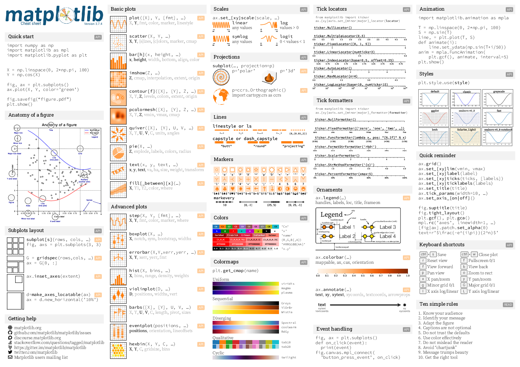
\begin{myboxed}{Quick start \hfill
\API{https://matplotlib.org/tutorials/introductory/pyplot.html}}
{\ttfamily \scriptsize
import numpy as np\\
import matplotlib as mpl\\
import matplotlib.pyplot as plt\\
\\
\\
X = np.linspace(0, 2*np.pi, 100)\\
Y = np.cos(X)\\
\\
fig, ax = plt.subplots()\\
ax.plot(X, Y, color='green')\\
\\
fig.savefig(``figure.pdf'')\\
plt.show() }
\end{myboxed}
\vspace{\fill}
% --- Figure anatomy --------------------------------------------------------
\begin{myboxed}{Anatomy of a figure}
\includegraphics[width=\columnwidth]{anatomy.pdf}
\end{myboxed}
\vspace{\fill}
% --- Layout ---------------------------------------------------------------
\begin{myboxed}{Subplots layout \hfill
\API{https://matplotlib.org/tutorials/intermediate/gridspec.html} }
\plot{layout-subplot.pdf}{\textbf{subplot[s]}(rows, cols, …)}
{https://matplotlib.org/stable/api/_as_gen/matplotlib.pyplot.subplots.html}
{\ttfamily fig, axs = plt.subplots(3, 3)}
{}
\plot{layout-gridspec.pdf}{G = \textbf{gridspec}(rows,cols, …)}
{https://matplotlib.org/stable/api/_as_gen/matplotlib.gridspec.GridSpec.html}
{\ttfamily ax = G[0, :]}{}
\plot{layout-inset.pdf}{ax.\textbf{inset\_axes}(extent)}
{https://matplotlib.org/stable/api/_as_gen/matplotlib.axes.Axes.inset_axes.html}
{}{}
\plot{layout-divider.pdf}{d=\textbf{make\_axes\_locatable}(ax)}
{https://matplotlib.org/mpl_toolkits/axes_grid/users/axes_divider.html}
{\ttfamily ax = d.new\_horizontal('10\%')}{}
\end{myboxed}
\vspace{\fill}
% --- Getting help ----------------------------------------------------------
\begin{myboxed}{Getting help}
\href{https://matplotlib.org}
{\faIcon{globe}\,matplotlib.org}\\
\href{https://github.com/matplotlib/matplotlib/issues}
{\faIcon{github}\,github.com/matplotlib/matplotlib/issues}\\
\href{https://discourse.matplotlib.org}
{\faIcon{discourse}\,discourse.matplotlib.org}\\
\href{https://stackoverflow.com/questions/tagged/matplotlib}
{\faIcon{stack-overflow}\,stackoverflow.com/questions/tagged/matplotlib}\\
\href{https://gitter.im/matplotlib/matplotlib}
{\faIcon{gitter}\,{https://gitter.im/matplotlib/matplotlib}}\\
\href{https://twitter.com/matplotlib}
{\faIcon{twitter}\,twitter.com/matplotlib}\\
\href{https://mail.python.org/mailman/listinfo/matplotlib-users}
{\faIcon[regular]{envelope}\,Matplotlib users mailing list}
\end{myboxed}
% --- Basic plots -----------------------------------------------------------
\begin{myboxed}{Basic plots}
\plot{basic-plot.pdf}{\textbf{plot}([X], Y, [fmt], …)}
{https://matplotlib.org/stable/api/_as_gen/matplotlib.pyplot.plot.html}
{\optional{X},
\mandatory{Y},
\optional{fmt},
\optional{color},
\optional{marker},
\optional{linestyle}}
{}
\plot{basic-scatter.pdf}{\textbf{scatter}(X, Y, …)}
{https://matplotlib.org/stable/api/_as_gen/matplotlib.pyplot.scatter.html}
{\mandatory{X},
\mandatory{Y},
\optional{[s]izes},
\optional{[c]olors},
\optional{marker},
\optional{cmap}}
{}
\plot{basic-bar.pdf}{\textbf{bar[h]}(x, height, …)}
{https://matplotlib.org/stable/api/_as_gen/matplotlib.pyplot.bar.html}
{ \mandatory{x},
\mandatory{height},
\optional{width},
\optional{bottom},
\optional{align},
\optional{color} }{}
\plot{basic-imshow.pdf}{\textbf{imshow}(Z, …)}
{https://matplotlib.org/stable/api/_as_gen/matplotlib.pyplot.imshow.html}
{ \mandatory{Z},
\optional{cmap},
\optional{interpolation},
\optional{extent},
\optional{origin} }
{}
\plot{basic-contour.pdf}{\textbf{contour[f]}([X], [Y], Z, …)}
{https://matplotlib.org/stable/api/_as_gen/matplotlib.pyplot.contour.html}
{ \optional{X},
\optional{Y},
\mandatory{Z},
\optional{levels},
\optional{colors},
\optional{extent},
\optional{origin} }
{}
\plot{basic-pcolormesh.pdf}{\textbf{pcolormesh}([X], [Y], Z, …)}
{https://matplotlib.org/stable/api/_as_gen/matplotlib.pyplot.pcolormesh.html}
{ \optional{X},
\optional{Y},
\mandatory{Z},
\optional{vmin},
\optional{vmax},
\optional{cmap}}
{}
\plot{basic-quiver.pdf}{\textbf{quiver}([X], [Y], U, V, …)}
{https://matplotlib.org/stable/api/_as_gen/matplotlib.pyplot.quiver.html}
{ \optional{X},
\optional{Y},
\mandatory{U},
\mandatory{V},
\optional{C},
\optional{units},
\optional{angles} }
{}
\plot{basic-pie.pdf}{\textbf{pie}(X, …)}
{https://matplotlib.org/stable/api/_as_gen/matplotlib.pyplot.pie.html}
{\mandatory{Z},
\optional{explode},
\optional{labels},
\optional{colors},
\optional{radius}}
{}
\plot{basic-text.pdf}{\textbf{text}(x, y, text, …)}
{https://matplotlib.org/stable/api/_as_gen/matplotlib.pyplot.text.html}
{\mandatory{x},
\mandatory{y},
\mandatory{text},
\optional{va},
\optional{ha},
\optional{size},
\optional{weight},
\optional{transform} }
{}
\plot{basic-fill.pdf}{\textbf{fill[\_between][x]}(…)}
{https://matplotlib.org/stable/api/_as_gen/matplotlib.pyplot.fill.html}
{\mandatory{X},
\optional{Y1},
\optional{Y2},
\optional{color},
\optional{where} }
{}
\end{myboxed}
\vspace{\fill}
% --- Advanced plots --------------------------------------------------------
\begin{myboxed}{Advanced plots}
\plot{advanced-step.pdf}{\textbf{step}(X, Y, [fmt], …)}
{https://matplotlib.org/stable/api/_as_gen/matplotlib.pyplot.step.html}
{\mandatory{X},
\mandatory{Y},
\optional{fmt},
\optional{color},
\optional{marker},
\optional{where} }
{}
\plot{advanced-boxplot.pdf}{\textbf{boxplot}(X, …)}
{https://matplotlib.org/stable/api/_as_gen/matplotlib.pyplot.boxplot.html}
{ \mandatory{X},
\optional{notch},
\optional{sym},
\optional{bootstrap},
\optional{widths} }
{}
\plot{advanced-errorbar.pdf}{\textbf{errorbar}(X,Y,xerr,yerr, …)}
{https://matplotlib.org/stable/api/_as_gen/matplotlib.pyplot.errorbar.html}
{ \mandatory{X},
\mandatory{Y},
\optional{xerr},
\optional{yerr},
\optional{fmt} }
{}
\plot{advanced-hist.pdf}{\textbf{hist}(X, bins, …)}
{https://matplotlib.org/stable/api/_as_gen/matplotlib.pyplot.hist.html}
{\mandatory{X},
\optional{bins},
\optional{range},
\optional{density},
\optional{weights}}
{}
\plot{advanced-violin.pdf}{\textbf{violinplot}(D, …)}
{https://matplotlib.org/stable/api/_as_gen/matplotlib.axes.Axes.violinplot.html}
{\mandatory{D},
\optional{positions},
\optional{widths},
\optional{vert} }
{}
\plot{advanced-barbs.pdf}{\textbf{barbs}([X], [Y], U, V, …)}
{https://matplotlib.org/stable/api/_as_gen/matplotlib.pyplot.barbs.html}
{ \optional{X},
\optional{Y},
\mandatory{U},
\mandatory{V},
\optional{C},
\optional{length},
\optional{pivot},
\optional{sizes} }
{}
\plot{advanced-event.pdf}{\textbf{eventplot}(positions, …)}
{https://matplotlib.org/stable/api/_as_gen/matplotlib.pyplot.eventplot.html}
{\mandatory{positions},
\optional{orientation},
\optional{lineoffsets} }
{}
\plot{advanced-hexbin.pdf}{\textbf{hexbin}(X, Y, C, …)}
{https://matplotlib.org/stable/api/_as_gen/matplotlib.pyplot.hexbin.html}
{\mandatory{X},
\mandatory{Y},
\optional{C},
\optional{gridsize},
\optional{bins} }
{}
\end{myboxed}
% --- Scale ---------------------------------------------------------------
\begin{myboxed}{Scales \hfill
\API{https://matplotlib.org/stable/api/scale_api.html}}
{\ttfamily ax.\textbf{set\_[xy]scale}(scale, …)}
\smallskip
\scale{scale-linear.pdf}{\textbf{linear}}{any values}
\scale{scale-log.pdf}{\textbf{log}}{values > 0}
\scale{scale-symlog.pdf}{\textbf{symlog}}{any values}
\scale{scale-logit.pdf}{\textbf{logit}}{0 < values < 1}
\end{myboxed}
%
\vspace{\fill}
%
% --- Projections -----------------------------------------------------------
\begin{myboxed}{Projections \hfill
\API{https://matplotlib.org/stable/api/projections_api.html}}
{\ttfamily \textbf{subplot}(…, projection=p)}
\smallskip
\scale{projection-polar.pdf}{p='polar'}{}
\scale{projection-3d.pdf}
{p='3d'\hfill\api{https://matplotlib.org/stable/api/toolkits/mplot3d.html}}{}
\plot{projection-cartopy.pdf}{p=ccrs.Orthographic()}
{https://scitools.org.uk/cartopy/docs/latest/reference/projections.html}
{import cartopy.crs as ccrs}
{}
\end{myboxed}
%
\vspace{\fill}
%
% --- Linestyles ---------------------------------------------------------------
\begin{myboxed}{Lines \hfill
\API{https://matplotlib.org/gallery/lines_bars_and_markers/linestyles.html}}
\includegraphics[width=\columnwidth]{linestyles.pdf}
\end{myboxed}
%
\vspace{\fill}
%
% --- Markers ---------------------------------------------------------------
\begin{myboxed}{Markers \hfill
\API{https://matplotlib.org/stable/api/markers_api.html}}
\includegraphics[width=\columnwidth]{markers.pdf}
\end{myboxed}
%
\vspace{\fill}
%
% --- Colors ---------------------------------------------------------------
\begin{myboxed}{Colors \hfill
\API{https://matplotlib.org/tutorials/colors/colors.html}}
% mpl.colors.to\_rbga(\textbf{color})\smallskip\\
\def\arraystretch{0.5}
\begin{tabular}{@{}p{0.7\columnwidth}p{0.25\columnwidth}@{}}
\palette{cycle}{'Cn'}
\palette{raw}{ 'x' }
\palette{name}{'name'}
\palette{rgba}{(R,G,B[,A])}
\palette{HexRGBA}{'\#RRGGBB[AA]'}
\palette{grey}{'x.y'}
\end{tabular}
\end{myboxed}
%
\vspace{\fill}
%
% --- Colormaps -------------------------------------------------------------
\begin{myboxed}{Colormaps \hfill
\API{https://matplotlib.org/tutorials/colors/colormaps.html}}
{\ttfamily plt.\textbf{get\_cmap}(name) \smallskip\\}
\def\arraystretch{0.5}
\begin{tabular}{@{}p{0.7\columnwidth}p{0.25\columnwidth}@{}}
\scriptsize \rule{0pt}{1.25em}Uniform & \\
\colormap{viridis} \colormap{magma} \colormap{plasma}
%
\scriptsize \rule{0pt}{1.25em}Sequential &\\
\colormap{Greys} \colormap{YlOrBr} \colormap{Wistia}
%
\scriptsize \rule{0pt}{1.25em}Diverging &\\
\colormap{Spectral} \colormap{coolwarm} \colormap{RdGy}
%
\scriptsize \rule{0pt}{1.25em}Qualitative &\\
\colormap{tab10} \colormap{tab20}
%
\scriptsize \rule{0pt}{1.25em}Cyclic &\\
\colormap{twilight} % \colormap{hsv}
\end{tabular}
\end{myboxed}
% --- Ticks locators --------------------------------------------------------
\begin{myboxed}{Tick locators \hfill
\API{https://matplotlib.org/stable/api/ticker_api.html}}
{\tiny \ttfamily
from matplotlib import ticker\\
ax.[xy]axis.set\_[minor|major]\_locator(\textbf{locator})\par
\vspace{1em}
\hspace{-1em}\includegraphics[width=\columnwidth]{tick-locators.pdf}
}
\end{myboxed}
%
\vspace{\fill}
%
\begin{myboxed}{Tick formatters \hfill
\API{https://matplotlib.org/stable/api/ticker_api.html}}
{\tiny \ttfamily
from matplotlib import ticker\\
ax.[xy]axis.set\_[minor|major]\_formatter(\textbf{formatter})\par
\vspace{1em}
\hspace{-1em}\includegraphics[width=\columnwidth]{tick-formatters.pdf}
}
\end{myboxed}
%
\vspace{\fill}
%
\begin{myboxed}{Ornaments}
{\ttfamily ax.\textbf{legend}(…) \hfill
\api{https://matplotlib.org/stable/api/_as_gen/matplotlib.pyplot.legend.html}}\\
handles, labels, loc, title, frameon\smallskip\\
\includegraphics[width=0.9\columnwidth]{legend.pdf}
\medskip\\
%
{\ttfamily ax.\textbf{colorbar}(…)} \hfill
\api{https://matplotlib.org/stable/api/_as_gen/matplotlib.pyplot.colorbar.html}\\
mappable, ax, cax, orientation \smallskip\\
\includegraphics[width=\columnwidth]{colorbar.pdf}\\
\medskip\\
%
{\ttfamily ax.\textbf{annotate}(…)} \hfill
\api{https://matplotlib.org/stable/api/_as_gen/matplotlib.pyplot.annotate.html}\\
\mandatory{text},
\mandatory{xy},
\mandatory{xytext},
\optional{xycoords},
\optional{textcoords},
\optional{arrowprops}
\smallskip\\
\includegraphics[width=\columnwidth]{annotate.pdf}\\
%
\end{myboxed}
%
\vspace{\fill}
%
\begin{myboxed}{Event handling \hfill
\API{https://matplotlib.org/users/event_handling.html}}
{\ttfamily \scriptsize
fig, ax = plt.subplots()\par
\par
def on\_click(event):\par
~~print(event)\par
fig.canvas.mpl\_connect(\par
~~'button\_press\_event', on\_click)\par
}
\end{myboxed}
%
% \vspace{\fill}
%
\begin{myboxed}{Animation \hfill
\API{https://matplotlib.org/stable/api/animation_api.html}}
{\ttfamily \scriptsize
import matplotlib.animation as mpla\par
~\par
T = np.linspace(0, 2*np.pi, 100)\par
S = np.sin(T)\par
line, = plt.plot(T, S)\par
def animate(i):\par
~~~~line.set\_ydata(np.sin(T+i/50))\par
anim = mpla.FuncAnimation(\par
~~~~plt.gcf(), animate, interval=5)\par
plt.show()\par
}
\end{myboxed}
%
\vspace{\fill}
%
\begin{myboxed}{Styles \hfill
\API{https://matplotlib.org/tutorials/introductory/customizing.html}}
\setlength{\fboxsep}{0pt}%
\setlength{\fboxrule}{.25pt}%
{\ttfamily plt.style.use(\textbf{style})\medskip}
\fbox{\includegraphics[width=.32\columnwidth]{style-default.pdf}}
\fbox{\includegraphics[width=.32\columnwidth]{style-classic.pdf}}
\fbox{\includegraphics[width=.32\columnwidth]{style-grayscale.pdf}}
\fbox{\includegraphics[width=.32\columnwidth]{style-ggplot.pdf}}
\fbox{\includegraphics[width=.32\columnwidth]{style-seaborn-v0_8.pdf}}
\fbox{\includegraphics[width=.32\columnwidth]{style-fast.pdf}}
\fbox{\includegraphics[width=.32\columnwidth]{style-bmh.pdf}}
\fbox{\includegraphics[width=.32\columnwidth]{style-Solarize_Light2.pdf}}
\fbox{\includegraphics[width=.32\columnwidth]{style-seaborn-v0_8-notebook.pdf}}
\end{myboxed}
%
\vspace{\fill}
%
\begin{myboxed}{Quick reminder}
{\ttfamily
ax.\textbf{grid}()\\
ax.\textbf{set\_[xy]lim}(vmin, vmax)\\
ax.\textbf{set\_[xy]label}(label)\\
ax.\textbf{set\_[xy]ticks}(ticks, [labels])\\
ax.\textbf{set\_[xy]ticklabels}(labels)\\
ax.\textbf{set\_title}(title)\\
ax.\textbf{tick\_params}(width=10, …)\\
ax.\textbf{set\_axis\_[on|off]}()\\
\\
fig.\textbf{suptitle}(title)\\
fig.\textbf{tight\_layout}()\\
plt.\textbf{gcf}(), plt.\textbf{gca}()\\
mpl.\textbf{rc}('axes', linewidth=1, …)\\
{[fig|ax]}.patch.\textbf{set\_alpha}(0)\\
\verb|text=r'$\frac{-e^{i\pi}}{2^n}$'|}
\end{myboxed}
%
\vspace{\fill}
%
%% % --- Toolkits --------------------------------------------------------------
%% \begin{myboxed}{Toolkits and libraries}
%% \href{https://matplotlib.org/basemap/}{Basemap} ---
%% \href{https://scitools.org.uk/cartopy/docs/latest/}{Cartopy} ---
%% \href{https://geopandas.org/}{GeoPandas} ---
%% \href{https://residentmario.github.io/geoplot/index.html}{Geoplot} ---
%% \href{https://github.com/yhat/ggpy}{GGPlot} ---
%% \href{http://holoviews.org/}{Holoviews} ---
%% \href{https://seaborn.pydata.org/}{Seaborn} ---
%% \href{https://gr-framework.org/}{GR Framework} ---
%% \href{https://www.scikit-yb.org/en/latest/}{Yellowbrick}
%% \end{myboxed}
%% %
%% \vspace{\fill}
%
\begin{myboxed}{Keyboard shortcuts \hfill
\API{https://matplotlib.org/users/navigation_toolbar.html}}
\def\arraystretch{1.25}
\begin{tabular}{ll}
\keys{\ctrl+s} Save & \keys{\ctrl+w} Close plot\\
\keys{r} Reset view & \keys{f} Fullscreen 0/1\\
\keys{f} View forward & \keys{b} View back\\
\keys{p} Pan view & \keys{o} Zoom to rect\\
\keys{x} X pan/zoom & \keys{y} Y pan/zoom\\
\keys{g} Minor grid 0/1 & \keys{G} Major grid 0/1\\
\keys{l} X axis log/linear & \keys{L} Y axis log/linear\\
%\keys{l} & Toggle y linear / log axis\\
\end{tabular}
\end{myboxed}
%
\vspace{\fill}
%
\begin{myboxed}{Ten simple rules \hfill
\READ{https://journals.plos.org/ploscompbiol/article?id=10.1371/journal.pcbi.1003833}}
1. Know your audience\\
2. Identify your message\\
3. Adapt the figure\\
4. Captions are not optional\\
5. Do not trust the defaults\\
6. Use color effectively\\
7. Do not mislead the reader\\
8. Avoid “chartjunk”\\
9. Message trumps beauty\\
10. Get the right tool
\end{myboxed}
\end{multicols*}
\begin{multicols*}{5}
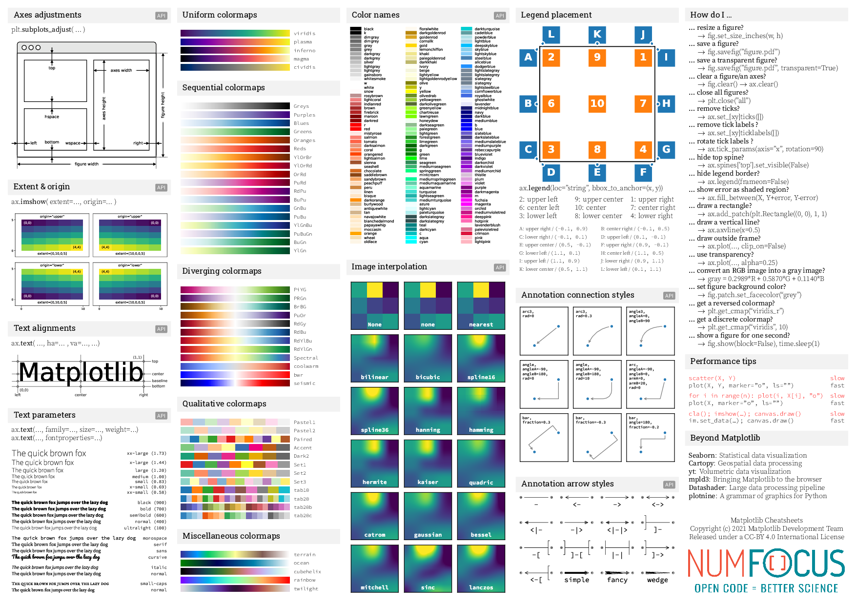
\begin{myboxed}{Axes adjustments\hfill
\API{https://matplotlib.org/stable/api/_as_gen/matplotlib.pyplot.subplots_adjust.html}}
plt.\textbf{subplots\_adjust}( … )\\
\includegraphics[width=\columnwidth]{adjustments.pdf}
\end{myboxed}
%
\vspace{\fill}
%
\begin{myboxed}{Extent \& origin \hfill
\API{https://matplotlib.org/tutorials/intermediate/imshow_extent.html} }
ax.\textbf{imshow}( extent=…, origin=… )\\
\includegraphics[width=\columnwidth]{extents.pdf}
\end{myboxed}
%
\vspace{\fill}
%
\begin{myboxed}{Text alignments \hfill
\API{https://matplotlib.org/tutorials/text/text_props.html} }
ax.\textbf{text}( …, ha=… , va=…, …)\\
\includegraphics[width=\columnwidth]{text-alignments.pdf}
\end{myboxed}
%
\vspace{\fill}
%
\begin{myboxed}{Text parameters \hfill
\API{https://matplotlib.org/tutorials/text/text_props.html}}
ax.\textbf{text}(…, family=…, size=…, weight=…)\\
ax.\textbf{text}(…, fontproperties=…)\\
\includegraphics[width=\columnwidth]{fonts.pdf}
\end{myboxed}
\begin{myboxed}{Uniform colormaps}
\begin{tabular}{@{}p{0.7\columnwidth}p{0.25\columnwidth}@{}}
\scriptsize \rule{0pt}{1.25em}\noindent
\colormap{viridis}
\colormap{plasma}
\colormap{inferno}
\colormap{magma}
\colormap{cividis}
\end{tabular}
\end{myboxed}
%
\vspace{\fill}
%
\begin{myboxed}{Sequential colormaps}
\begin{tabular}{@{}p{0.7\columnwidth}p{0.25\columnwidth}@{}}
\scriptsize \rule{0pt}{1.25em}\noindent
\colormap{Greys}
\colormap{Purples}
\colormap{Blues}
\colormap{Greens}
\colormap{Oranges}
\colormap{Reds}
\colormap{YlOrBr}
\colormap{YlOrRd}
\colormap{OrRd}
\colormap{PuRd}
\colormap{RdPu}
\colormap{BuPu}
\colormap{GnBu}
\colormap{PuBu}
\colormap{YlGnBu}
\colormap{PuBuGn}
\colormap{BuGn}
\colormap{YlGn}
\end{tabular}
\end{myboxed}
%
\vspace{\fill}
%
\begin{myboxed}{Diverging colormaps}
\begin{tabular}{@{}p{0.7\columnwidth}p{0.25\columnwidth}@{}}
\scriptsize \rule{0pt}{1.25em}\noindent
\colormap{PiYG}
\colormap{PRGn}
\colormap{BrBG}
\colormap{PuOr}
\colormap{RdGy}
\colormap{RdBu}
\colormap{RdYlBu}
\colormap{RdYlGn}
\colormap{Spectral}
\colormap{coolwarm}
\colormap{bwr}
\colormap{seismic}
\end{tabular}
\end{myboxed}
%
\vspace{\fill}
%
\begin{myboxed}{Qualitative colormaps}
\begin{tabular}{@{}p{0.7\columnwidth}p{0.25\columnwidth}@{}}
\scriptsize \rule{0pt}{1.25em}\noindent
\colormap{Pastel1}
\colormap{Pastel2}
\colormap{Paired}
\colormap{Accent}
\colormap{Dark2}
\colormap{Set1}
\colormap{Set2}
\colormap{Set3}
\colormap{tab10}
\colormap{tab20}
\colormap{tab20b}
\colormap{tab20c}
\end{tabular}
\end{myboxed}
%
\vspace{\fill}
%
\begin{myboxed}{Miscellaneous colormaps}
\begin{tabular}{@{}p{0.7\columnwidth}p{0.25\columnwidth}@{}}
\scriptsize \rule{0pt}{1.25em}\noindent
\colormap{terrain}
\colormap{ocean}
\colormap{cubehelix}
\colormap{rainbow}
\colormap{twilight}
\end{tabular}
\end{myboxed}
\begin{myboxed}{Color names \hfill
\API{https://matplotlib.org/stable/api/colors_api.html} }
\includegraphics[width=\columnwidth]{colornames.pdf}
\end{myboxed}
%
\vspace{\fill}
%
\begin{myboxed}{Image interpolation
\hfill \API{https://matplotlib.org/gallery/images_contours_and_fields/interpolation_methods.html} }
\smallskip
%% plt.\textbf{imshow}(…, interpolation=…)\\
%% plt.\textbf{contour[f]}(…, interpolation=…)\\
\includegraphics[width=\columnwidth]{interpolations.pdf}
\end{myboxed}
\begin{myboxed}{Legend placement}
\includegraphics[width=\columnwidth]{legend-placement.pdf}
ax.\textbf{legend}(loc="string", bbox\_to\_anchor=(x, y))\\
\begin{tabular}{@{}p{0.33\columnwidth}
p{0.33\columnwidth}
p{0.33\columnwidth}@{}}
\scriptsize \rule{0pt}{1.25em}\noindent
2: upper left & 9: upper center & 1: upper right\\
6: center left & 10: center & 7: center right\\
3: lower left & 8: lower center & 4: lower right\\
\end{tabular}
\begin{tabular}{@{}p{0.495\columnwidth}
p{0.495\columnwidth}@{}}
\scriptsize \rule{0pt}{1.25em}\noindent
\tiny A: upper right / {\ttfamily (-0.1, 0.9)} & \tiny B: center right / {\ttfamily (-0.1, 0.5)}\\
\tiny C: lower right / {\ttfamily (-0.1, 0.1)} & \tiny D: upper left / {\ttfamily (0.1, -0.1)}\\
\tiny E: upper center / {\ttfamily (0.5, -0.1)} & \tiny F: upper right / {\ttfamily (0.9, -0.1)}\\
\tiny G: lower left / {\ttfamily (1.1, 0.1)} & \tiny H: center left / {\ttfamily (1.1, 0.5)}\\
\tiny I: upper left / {\ttfamily (1.1, 0.9)} & \tiny J: lower right / {\ttfamily (0.9, 1.1)}\\
\tiny K: lower center / {\ttfamily (0.5, 1.1)} & \tiny L: lower left / {\ttfamily (0.1, 1.1)}
\end{tabular}
\end{myboxed}
%
\vspace{\fill}
%
\begin{myboxed}{Annotation connection styles \hfill
\API{https://matplotlib.org/tutorials/text/annotations.html} }
\includegraphics[width=\columnwidth]{annotation-connection-styles.pdf}
\end{myboxed}
%
\vspace{\fill}
%
\begin{myboxed}{Annotation arrow styles \hfill
\API{https://matplotlib.org/tutorials/text/annotations.html} }
\includegraphics[width=\columnwidth]{annotation-arrow-styles.pdf}
\end{myboxed}
%
\vspace{\fill}
%
%
\begin{myboxed}{How do I …}
\textbf{… resize a figure?}\\
\hspace*{2.5mm}~$\rightarrow$ fig.set\_size\_inches(w, h)\\
\textbf{… save a figure?}\\
\hspace*{2.5mm}~$\rightarrow$ fig.savefig("figure.pdf")\\
\textbf{… save a transparent figure?}\\
\hspace*{2.5mm}~$\rightarrow$ fig.savefig("figure.pdf", transparent=True)\\
\textbf{… clear a figure/an axes?}\\
\hspace*{2.5mm}~$\rightarrow$ fig.clear() $\rightarrow$ ax.clear()\\
\textbf{… close all figures?}\\
\hspace*{2.5mm}~$\rightarrow$ plt.close("all")\\
\textbf{… remove ticks?}\\
\hspace*{2.5mm}~$\rightarrow$ ax.set\_[xy]ticks([])\\
\textbf{… remove tick labels ?}\\
\hspace*{2.5mm}~$\rightarrow$ ax.set\_[xy]ticklabels([])\\
\textbf{… rotate tick labels ?}\\
\hspace*{2.5mm}~$\rightarrow$ ax.tick\_params(axis="x", rotation=90)\\
\textbf{… hide top spine?}\\
\hspace*{2.5mm}~$\rightarrow$ ax.spines['top'].set\_visible(False)\\
\textbf{… hide legend border?}\\
\hspace*{2.5mm}~$\rightarrow$ ax.legend(frameon=False)\\
\textbf{… show error as shaded region?}\\
\hspace*{2.5mm}~$\rightarrow$ ax.fill\_between(X, Y+error, Y-error)\\
\textbf{… draw a rectangle?}\\
\hspace*{2.5mm}~$\rightarrow$ ax.add\_patch(plt.Rectangle((0, 0), 1, 1)\\
\textbf{… draw a vertical line?}\\
\hspace*{2.5mm}~$\rightarrow$ ax.axvline(x=0.5)\\
\textbf{… draw outside frame?}\\
\hspace*{2.5mm}~$\rightarrow$ ax.plot(…, clip\_on=False)\\
\textbf{… use transparency?}\\
\hspace*{2.5mm}~$\rightarrow$ ax.plot(…, alpha=0.25)\\
\textbf{… convert an RGB image into a gray image? }\\
\hspace*{2.5mm}~$\rightarrow$ gray = 0.2989*R + 0.5870*G + 0.1140*B\\
\textbf{… set figure background color?}\\
\hspace*{2.5mm}~$\rightarrow$ fig.patch.set\_facecolor(``grey'')\\
\textbf{… get a reversed colormap?}\\
\hspace*{2.5mm}~$\rightarrow$ plt.get\_cmap(``viridis\_r'')\\
\textbf{… get a discrete colormap?}\\
\hspace*{2.5mm}~$\rightarrow$ plt.get\_cmap(``viridis'', 10)\\
\textbf{… show a figure for one second?}\\
\hspace*{2.5mm}~$\rightarrow$ fig.show(block=False), time.sleep(1)
\end{myboxed}
%
\vspace{\fill}
%
\begin{myboxed}{Performance tips}
\smallskip
{\ttfamily \fontsize{6pt}{7pt}\selectfont
%
\textcolor{red}{scatter(X, Y) \hfill slow}\\
plot(X, Y, marker="o", ls="") \hfill fast%
\vskip.5\baselineskip
%
\textcolor{red}{for i in range(n): plot(i, X[i], "o") \hfill slow}\\
plot(X, marker="o", ls="") \hfill fast%
\vskip.5\baselineskip
%
\textcolor{red}{cla(); imshow(…); canvas.draw() \hfill slow}\\
im.set\_data(…); canvas.draw() \hfill fast%
\vskip.1\baselineskip
}
\end{myboxed}
%
\vspace{\fill}
%
\begin{myboxed}{Beyond Matplotlib}
\smallskip
\href{https://seaborn.pydata.org/}{\textbf{Seaborn}}: Statistical data visualization\\
\href{https://scitools.org.uk/cartopy/docs/latest/}{\textbf{Cartopy}}: Geospatial data processing\\
\href{https://yt-project.org/doc/index.html}{\textbf{yt}}: Volumetric data visualization\\
\href{https://mpld3.github.io}{\textbf{mpld3}}: Bringing Matplotlib to the browser\\
\href{https://datashader.org/}{\textbf{Datashader}}: Large data processing pipeline\\
\href{https://plotnine.org/}{\textbf{plotnine}}: A grammar of graphics for Python
\end{myboxed}
%
\begin{center}
\href{https://github.com/matplotlib/cheatsheets}{Matplotlib Cheatsheets}\\
Copyright (c) 2021 Matplotlib Development Team\\
Released under a CC-BY 4.0 International License\\
\smallskip
\includegraphics[width=\columnwidth]{numfocus.png}
\end{center}
\end{multicols*}
\end{document}
================================================
FILE: check-diffs.py
================================================
#!/usr/bin/env python
import os
import subprocess
import sys
from pathlib import Path
ROOT_DIR = Path(__file__).parent
if os.environ.get('GITHUB_ACTIONS', '') == '':
print('Not running when not in GitHub Actions.')
sys.exit()
summary_file = os.environ.get('GITHUB_STEP_SUMMARY')
if summary_file is None:
sys.exit('$GITHUB_STEP_SUMMARY is not set')
gh_pages = ROOT_DIR.parent / 'pages'
subprocess.run(['git', 'fetch', 'https://github.com/matplotlib/cheatsheets.git',
'gh-pages:upstream-gh-pages'], check=True)
subprocess.run(['git', 'worktree', 'add', gh_pages, 'upstream-gh-pages'],
check=True)
diff_dir = ROOT_DIR / 'diffs'
diff_dir.mkdir(exist_ok=True)
hashes = {}
for original in gh_pages.glob('*.png'):
result = subprocess.run(
['compare', '-metric', 'PHASH',
original,
ROOT_DIR / 'docs/_build/html' / original.name,
diff_dir / f'{original.stem}-diff.png'],
text=True, stderr=subprocess.PIPE)
if result.returncode == 2: # Some kind of IO or similar error.
hashes[original] = (float('nan'), result.stderr)
elif result.stderr: # Images were different.
hashes[original] = (float(result.stderr), '')
else: # No differences.
hashes[original] = (0.0, '')
with open(summary_file, 'w+') as summary:
print('# Cheatsheet image comparison', file=summary)
print('| Filename | Perceptual Hash Difference | Error message |', file=summary)
print('| -------- | -------------------------- | ------------- |', file=summary)
for filename, (hash, message) in sorted(hashes.items()):
message = message.replace('\n', ' ').replace('|', '\\|')
print(f'| {filename.name} | {hash:.05f} | {message}', file=summary)
print(file=summary)
subprocess.run(['git', 'worktree', 'remove', gh_pages])
================================================
FILE: check-links.py
================================================
#!/usr/bin/env python
import sys
import pdfx
pdf = pdfx.PDFx(sys.argv[1])
refs = [ref for ref in pdf.get_references() if ref.reftype == 'url']
status_codes = [pdfx.downloader.get_status_code(ref.ref) for ref in refs]
broken_links = [(ref.ref, code) for ref, code in zip(refs, status_codes) if code != 200]
# it seems that Twitter does not respond well to the link checker and throws a 400
if all(['twitter.com' in url for url, _ in broken_links]):
sys.exit(0)
else:
print('Broken links:', broken_links)
sys.exit(1)
================================================
FILE: check-matplotlib-version.py
================================================
#!/usr/bin/env python
import matplotlib as mpl
assert mpl.__version__ == '3.9.4'
================================================
FILE: check-num-pages.sh
================================================
#!/bin/bash
#
# Check that a given pdf has a certain number of pages.
# Usage:
# check-num-pages.sh [pdffile] [num_pages]
set -x
pdffile=$1
num_pages=$2
[[ "$(pdfinfo $pdffile | grep Pages | awk '{print $2}')" == "$num_pages" ]] || exit 1
================================================
FILE: docs/Makefile
================================================
# Minimal makefile for Sphinx documentation
#
# You can set these variables from the command line, and also
# from the environment for the first two.
SPHINXOPTS ?= -W
SPHINXBUILD ?= sphinx-build
SOURCEDIR = .
BUILDDIR = _build
# Put it first so that "make" without argument is like "make help".
help:
@$(SPHINXBUILD) -M help "$(SOURCEDIR)" "$(BUILDDIR)" $(SPHINXOPTS) $(O)
show:
@python -c "import webbrowser; webbrowser.open_new_tab('file://$(shell pwd)/build/html/index.html')"
.PHONY: help Makefile
# Catch-all target: route all unknown targets to Sphinx using the new
# "make mode" option. $(O) is meant as a shortcut for $(SPHINXOPTS).
%: Makefile
@$(SPHINXBUILD) -M $@ "$(SOURCEDIR)" "$(BUILDDIR)" $(SPHINXOPTS) $(O)
================================================
FILE: docs/conf.py
================================================
import datetime
# -- Project information -----------------------------------------------------
html_title = 'Visualization with Python'
project = "Matplotlib cheatsheets"
copyright = (
f"2012 - {datetime.datetime.now().year} The Matplotlib development team"
)
author = "Matplotlib Developers"
# -- General configuration ---------------------------------------------------
# Add any Sphinx extension module names here, as strings. They can be
# extensions coming with Sphinx (named 'sphinx.ext.*') or your custom
# ones.
extensions = ["sphinx_design"]
# Add any paths that contain templates here, relative to this directory.
templates_path = []
# List of patterns, relative to source directory, that match files and
# directories to ignore when looking for source files.
# This pattern also affects html_static_path and html_extra_path.
exclude_patterns = ["_build", "Thumbs.db", ".DS_Store"]
# -- Options for HTML output -------------------------------------------------
html_css_files = ['css/normalize.css', 'css/landing.css']
html_theme = "mpl_sphinx_theme"
html_favicon = "_static/favicon.ico"
html_theme_options = {
"navbar_links": ("absolute", "server-stable"),
}
html_sidebars = {
"**": []
}
# Add any paths that contain custom static files (such as style sheets) here,
# relative to this directory. They are copied after the theme static files,
# so a file named "default.css" will overwrite the theme's "default.css".
html_static_path = ["_static"]
================================================
FILE: docs/index.rst
================================================
.. title:: Matplotlib cheatsheets
***********************************
Matplotlib cheatsheets and handouts
***********************************
Cheatsheets
***********
.. grid:: 2
.. grid-item::
.. image:: ../cheatsheets-1.png
:width: 270px
:align: center
:alt: image of first page of cheatsheets
.. grid-item::
.. image:: ../cheatsheets-2.png
:width: 270px
:align: center
:alt: image of second page of cheatsheets
`Cheatsheets [pdf] <./cheatsheets.pdf>`_
Handouts
********
.. grid:: 1 2 3 3
.. grid-item::
.. image:: ../handout-beginner.png
:width: 270px
:align: center
:alt: image of beginner handout
`Beginner [pdf] <./handout-beginner.pdf>`_
.. grid-item::
.. image:: ../handout-intermediate.png
:width: 270px
:align: center
:alt: image of intermediate handout
`Intermediate [pdf] <./handout-intermediate.pdf>`_
.. grid-item::
.. image:: ../handout-tips.png
:width: 270px
:align: center
:alt: image of tips handout
`Tips [pdf] <./handout-tips.pdf>`_
Contribute
**********
Issues, suggestions, or pull-requests gratefully accepted at
`matplotlib/cheatsheets `_
================================================
FILE: fonts/.gitignore
================================================
.uuid
================================================
FILE: fonts/Makefile
================================================
FONT_DIRS := eb-garamond roboto roboto-mono roboto-slab source-code-pro source-sans-pro source-serif-pro pacifico
EB_GARAMOND_ZIP := https://bitbucket.org/georgd/eb-garamond/downloads/EBGaramond-0.016.zip
ROBOTO_ZIP := https://github.com/googlefonts/roboto/releases/download/v2.138/roboto-unhinted.zip
ROBOTO_MONO_ZIP := https://github.com/googlefonts/RobotoMono/archive/8f651634e746da6df6c2c0be73255721d24f2372.zip
ROBOTO_SLAB_ZIP := https://github.com/googlefonts/robotoslab/archive/a65e6d00d8e3e7ee2fabef844e58fa12690384d2.zip
SOURCE_CODE_PRO_ZIP := https://github.com/adobe-fonts/source-code-pro/releases/download/2.038R-ro%2F1.058R-it%2F1.018R-VAR/OTF-source-code-pro-2.038R-ro-1.058R-it.zip
SOURCE_SANS_PRO_ZIP := https://github.com/adobe-fonts/source-sans/releases/download/2.045R-ro%2F1.095R-it/source-sans-pro-2.045R-ro-1.095R-it.zip
SOURCE_SERIF_PRO_ZIP := https://github.com/adobe-fonts/source-serif/releases/download/3.001R/source-serif-pro-3.001R.zip
PACIFICO := https://raw.githubusercontent.com/googlefonts/Pacifico/refs/heads/main/fonts/ttf/Pacifico-Regular.ttf
UNZIP_FLAGS := -x "__MACOSX/*"
.PHONY: default
default: all
.PHONY: all
all: sources
mkdir -p $(FONT_DIRS)
cd eb-garamond && unzip -j /tmp/eb-garamond.zip "EBGaramond-0.016/otf/*.otf" $(UNZIP_FLAGS)
cd roboto && unzip -j /tmp/roboto.zip "*.ttf" $(UNZIP_FLAGS)
cd roboto-mono && unzip -j /tmp/roboto-mono.zip "RobotoMono-8f651634e746da6df6c2c0be73255721d24f2372/fonts/ttf/*.ttf" $(UNZIP_FLAGS)
cd roboto-slab && unzip -j /tmp/roboto-slab.zip "robotoslab-a65e6d00d8e3e7ee2fabef844e58fa12690384d2/fonts/static/*.ttf" $(UNZIP_FLAGS)
cd source-code-pro && unzip -j /tmp/source-code-pro.zip "*.otf" $(UNZIP_FLAGS)
cd source-sans-pro && unzip -j /tmp/source-sans-pro.zip "source-sans-pro-2.045R-ro-1.095R-it/OTF/*.otf" $(UNZIP_FLAGS)
cd source-serif-pro && unzip -j /tmp/source-serif-pro.zip "source-serif-pro-3.001R/OTF/*.otf" $(UNZIP_FLAGS)
cd pacifico && cp /tmp/pacifico.ttf .
.PHONY: sources
sources:
wget $(EB_GARAMOND_ZIP) -O /tmp/eb-garamond.zip
wget $(ROBOTO_ZIP) -O /tmp/roboto.zip
wget $(ROBOTO_MONO_ZIP) -O /tmp/roboto-mono.zip
wget $(ROBOTO_SLAB_ZIP) -O /tmp/roboto-slab.zip
wget $(SOURCE_CODE_PRO_ZIP) -O /tmp/source-code-pro.zip
wget $(SOURCE_SANS_PRO_ZIP) -O /tmp/source-sans-pro.zip
wget $(SOURCE_SERIF_PRO_ZIP) -O /tmp/source-serif-pro.zip
wget $(PACIFICO) -O /tmp/pacifico.ttf
.PHONY: clean
clean:
- rm $(HOME)/.cache/matplotlib/fontlist*
- rm -rf $(FONT_DIRS)
================================================
FILE: handout-beginner.tex
================================================
\documentclass[10pt,landscape,a4paper]{article}
\usepackage[right=10mm, left=10mm, top=10mm, bottom=10mm]{geometry}
\usepackage[utf8]{inputenc}
\usepackage[T1]{fontenc}
\usepackage[english]{babel}
\usepackage[rm,light]{roboto}
\usepackage{xcolor}
\usepackage{graphicx}
\graphicspath{{./figures/}}
\usepackage{multicol}
\usepackage{colortbl}
\usepackage{array}
\setlength\parindent{0pt}
\setlength{\tabcolsep}{2pt}
\baselineskip=0pt
\setlength\columnsep{1em}
\definecolor{Gray}{gray}{0.85}
% --- Listing -----------------------------------------------------------------
\usepackage{listings}
\lstset{
frame=tb, framesep=4pt, framerule=0pt,
backgroundcolor=\color{black!5},
basicstyle=\ttfamily,
commentstyle=\ttfamily\color{black!50},
breakatwhitespace=false,
breaklines=true,
extendedchars=true,
keepspaces=true,
language=Python,
rulecolor=\color{black},
showspaces=false,
showstringspaces=false,
showtabs=false,
tabsize=2,
%
emph = { plot, scatter, imshow, bar, contourf, pie, subplots, show, savefig,
errorbar, boxplot, hist, set_title, set_xlabel, set_ylabel, suptitle, },
emphstyle = {\ttfamily\bfseries}
}
% --- Fonts -------------------------------------------------------------------
\usepackage{fontspec}
\usepackage[babel=true]{microtype}
\defaultfontfeatures{Ligatures = TeX, Mapping = tex-text}
\setsansfont{Roboto} [ Path = fonts/roboto/Roboto-,
Extension = .ttf,
UprightFont = Light,
ItalicFont = LightItalic,
BoldFont = Regular,
BoldItalicFont = Italic ]
\setromanfont{RobotoSlab} [ Path = fonts/roboto-slab/RobotoSlab-,
Extension = .ttf,
UprightFont = Light,
BoldFont = Bold ]
\setmonofont{RobotoMono} [ Path = fonts/roboto-mono/RobotoMono-,
Extension = .ttf,
Scale = 0.90,
UprightFont = Light,
ItalicFont = LightItalic,
BoldFont = Regular,
BoldItalicFont = Italic ]
\renewcommand{\familydefault}{\sfdefault}
% -----------------------------------------------------------------------------
\begin{document}
\thispagestyle{empty}
\section*{\LARGE \rmfamily
Matplotlib \textcolor{orange}{\mdseries for beginners}}
\begin{multicols*}{3}
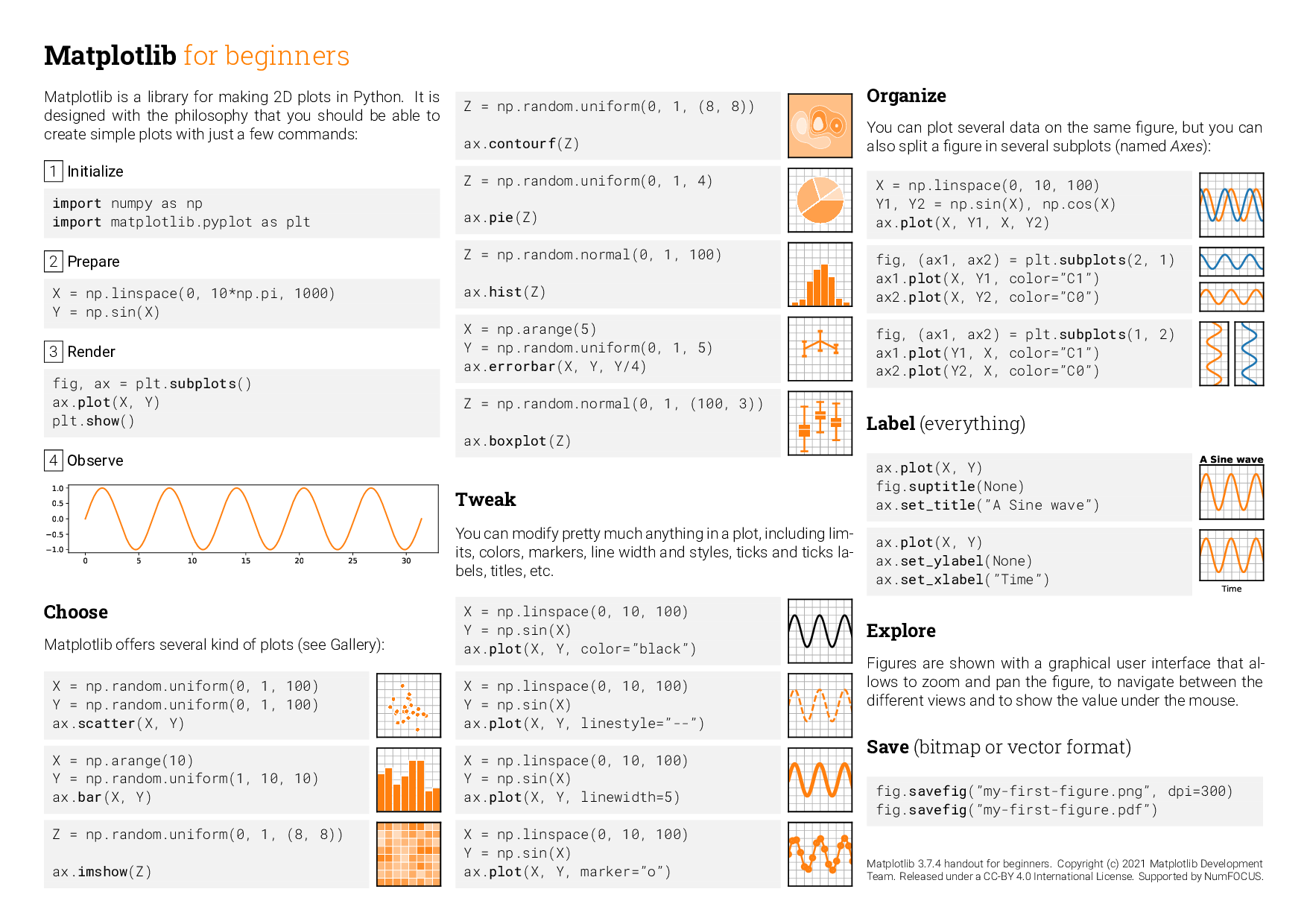
Matplotlib is a library for making 2D plots in Python. It is designed
with the philosophy that you should be able to create simple plots
with just a few commands:\\
\fbox{1} \textbf{Initialize}
\begin{lstlisting}
import numpy as np
import matplotlib.pyplot as plt
\end{lstlisting}
%
\fbox{2} \textbf{Prepare}
\begin{lstlisting}
X = np.linspace(0, 10*np.pi, 1000)
Y = np.sin(X)
\end{lstlisting}
%
\fbox{3} \textbf{Render}
\begin{lstlisting}
fig, ax = plt.subplots()
ax.plot(X, Y)
plt.show()
\end{lstlisting}
%
\fbox{4} \textbf{Observe} \medskip\\
\includegraphics[width=\linewidth]{sine.pdf}
% -----------------------------------------------------------------------------
\subsection*{\rmfamily Choose}
% -----------------------------------------------------------------------------
Matplotlib offers several kind of plots (see Gallery): \medskip
\begin{tabular}{@{}m{.821\linewidth}m{.169\linewidth}}
\begin{lstlisting}[belowskip=-\baselineskip]
X = np.random.uniform(0, 1, 100)
Y = np.random.uniform(0, 1, 100)
ax.scatter(X, Y)
\end{lstlisting}
& \raisebox{-0.75em}{\includegraphics[width=\linewidth]{basic-scatter.pdf}}
\end{tabular}
% -----------------------------------------------------------------------------
\begin{tabular}{@{}m{.821\linewidth}m{.169\linewidth}}
\begin{lstlisting}[belowskip=-\baselineskip]
X = np.arange(10)
Y = np.random.uniform(1, 10, 10)
ax.bar(X, Y)
\end{lstlisting}
& \raisebox{-0.75em}{\includegraphics[width=\linewidth]{basic-bar.pdf}}
\end{tabular}
% -----------------------------------------------------------------------------
\begin{tabular}{@{}m{.821\linewidth}m{.169\linewidth}}
\begin{lstlisting}[belowskip=-\baselineskip]
Z = np.random.uniform(0, 1, (8, 8))
ax.imshow(Z)
\end{lstlisting}
& \raisebox{-0.75em}{\includegraphics[width=\linewidth]{basic-imshow.pdf}}
\end{tabular}
% -----------------------------------------------------------------------------
\begin{tabular}{@{}m{.821\linewidth}m{.169\linewidth}}
\begin{lstlisting}[belowskip=-\baselineskip]
Z = np.random.uniform(0, 1, (8, 8))
ax.contourf(Z)
\end{lstlisting}
& \raisebox{-0.75em}{\includegraphics[width=\linewidth]{basic-contour.pdf}}
\end{tabular}
% -----------------------------------------------------------------------------
\begin{tabular}{@{}m{.821\linewidth}m{.169\linewidth}}
\begin{lstlisting}[belowskip=-\baselineskip]
Z = np.random.uniform(0, 1, 4)
ax.pie(Z)
\end{lstlisting}
& \raisebox{-0.75em}{\includegraphics[width=\linewidth]{basic-pie.pdf}}
\end{tabular}
% -----------------------------------------------------------------------------
\begin{tabular}{@{}m{.821\linewidth}m{.169\linewidth}}
\begin{lstlisting}[belowskip=-\baselineskip]
Z = np.random.normal(0, 1, 100)
ax.hist(Z)
\end{lstlisting}
& \raisebox{-0.75em}{\includegraphics[width=\linewidth]{advanced-hist.pdf}}
\end{tabular}
% -----------------------------------------------------------------------------
\begin{tabular}{@{}m{.821\linewidth}m{.169\linewidth}}
\begin{lstlisting}[belowskip=-\baselineskip]
X = np.arange(5)
Y = np.random.uniform(0, 1, 5)
ax.errorbar(X, Y, Y/4)
\end{lstlisting}
& \raisebox{-0.75em}{\includegraphics[width=\linewidth]{advanced-errorbar.pdf}}
\end{tabular}
% -----------------------------------------------------------------------------
\begin{tabular}{@{}m{.821\linewidth}m{.169\linewidth}}
\begin{lstlisting}[belowskip=-\baselineskip]
Z = np.random.normal(0, 1, (100, 3))
ax.boxplot(Z)
\end{lstlisting}
& \raisebox{-0.75em}{\includegraphics[width=\linewidth]{advanced-boxplot.pdf}}
\end{tabular}
% -----------------------------------------------------------------------------
\subsection*{\rmfamily Tweak}
% -----------------------------------------------------------------------------
You can modify pretty much anything in a plot, including limits,
colors, markers, line width and styles, ticks and ticks labels,
titles, etc. \medskip
% -----------------------------------------------------------------------------
\begin{tabular}{@{}m{.821\linewidth}m{.169\linewidth}}
\begin{lstlisting}[belowskip=-\baselineskip]
X = np.linspace(0, 10, 100)
Y = np.sin(X)
ax.plot(X, Y, color="black")
\end{lstlisting}
& \raisebox{-0.75em}{\includegraphics[width=\linewidth]{plot-color.pdf}}
\end{tabular}
% -----------------------------------------------------------------------------
\begin{tabular}{@{}m{.821\linewidth}m{.169\linewidth}}
\begin{lstlisting}[belowskip=-\baselineskip]
X = np.linspace(0, 10, 100)
Y = np.sin(X)
ax.plot(X, Y, linestyle="--")
\end{lstlisting}
& \raisebox{-0.75em}{\includegraphics[width=\linewidth]{plot-linestyle.pdf}}
\end{tabular}
% -----------------------------------------------------------------------------
\begin{tabular}{@{}m{.821\linewidth}m{.169\linewidth}}
\begin{lstlisting}[belowskip=-\baselineskip]
X = np.linspace(0, 10, 100)
Y = np.sin(X)
ax.plot(X, Y, linewidth=5)
\end{lstlisting}
& \raisebox{-0.75em}{\includegraphics[width=\linewidth]{plot-linewidth.pdf}}
\end{tabular}
% -----------------------------------------------------------------------------
\begin{tabular}{@{}m{.821\linewidth}m{.169\linewidth}}
\begin{lstlisting}[belowskip=-\baselineskip]
X = np.linspace(0, 10, 100)
Y = np.sin(X)
ax.plot(X, Y, marker="o")
\end{lstlisting}
& \raisebox{-0.75em}{\includegraphics[width=\linewidth]{plot-marker.pdf}}
\end{tabular}
% -----------------------------------------------------------------------------
\subsection*{\rmfamily Organize}
% -----------------------------------------------------------------------------
You can plot several data on the same figure, but you can also split a figure
in several subplots (named {\em Axes}): \medskip
% -----------------------------------------------------------------------------
\begin{tabular}{@{}m{.821\linewidth}m{.169\linewidth}}
\begin{lstlisting}[belowskip=-\baselineskip]
X = np.linspace(0, 10, 100)
Y1, Y2 = np.sin(X), np.cos(X)
ax.plot(X, Y1, X, Y2)
\end{lstlisting}
& \raisebox{-0.75em}{\includegraphics[width=\linewidth]{plot-multi.pdf}}
\end{tabular}
% -----------------------------------------------------------------------------
\begin{tabular}{@{}m{.821\linewidth}m{.169\linewidth}}
\begin{lstlisting}[belowskip=-\baselineskip]
fig, (ax1, ax2) = plt.subplots(2, 1)
ax1.plot(X, Y1, color="C1")
ax2.plot(X, Y2, color="C0")
\end{lstlisting}
& \raisebox{-0.75em}{\includegraphics[width=\linewidth]{plot-vsplit.pdf}}
\end{tabular}
% -----------------------------------------------------------------------------
\begin{tabular}{@{}m{.821\linewidth}m{.169\linewidth}}
\begin{lstlisting}[belowskip=-\baselineskip]
fig, (ax1, ax2) = plt.subplots(1, 2)
ax1.plot(Y1, X, color="C1")
ax2.plot(Y2, X, color="C0")
\end{lstlisting}
& \raisebox{-0.75em}{\includegraphics[width=\linewidth]{plot-hsplit.pdf}}
\end{tabular}
% -----------------------------------------------------------------------------
\subsection*{\rmfamily Label \mdseries (everything)}
% -----------------------------------------------------------------------------
% -----------------------------------------------------------------------------
\begin{tabular}{@{}m{.821\linewidth}m{.169\linewidth}}
\begin{lstlisting}[belowskip=-\baselineskip]
ax.plot(X, Y)
fig.suptitle(None)
ax.set_title("A Sine wave")
\end{lstlisting}
& \raisebox{-0.75em}{\includegraphics[width=\linewidth]{plot-title.pdf}}
\end{tabular}
% -----------------------------------------------------------------------------
\begin{tabular}{@{}m{.821\linewidth}m{.169\linewidth}}
\begin{lstlisting}[belowskip=-\baselineskip]
ax.plot(X, Y)
ax.set_ylabel(None)
ax.set_xlabel("Time")
\end{lstlisting}
& \raisebox{-0.75em}{\includegraphics[width=\linewidth]{plot-xlabel.pdf}}
\end{tabular}
% -----------------------------------------------------------------------------
\subsection*{\rmfamily Explore}
% -----------------------------------------------------------------------------
Figures are shown with a graphical user interface that allows to zoom
and pan the figure, to navigate between the different views and to
show the value under the mouse.
% -----------------------------------------------------------------------------
\subsection*{\rmfamily Save \mdseries (bitmap or vector format)}
% -----------------------------------------------------------------------------
\begin{lstlisting}[belowskip=-\baselineskip]
fig.savefig("my-first-figure.png", dpi=300)
fig.savefig("my-first-figure.pdf")
\end{lstlisting}
%
\vfill
%
{\scriptsize
Matplotlib 3.9.4 handout for beginners.
Copyright (c) 2021 Matplotlib Development Team.
Released under a CC-BY 4.0 International License.
Supported by NumFOCUS.
\par}
\end{multicols*}
\end{document}
================================================
FILE: handout-intermediate.tex
================================================
\documentclass[10pt,landscape,a4paper]{article}
\usepackage[right=10mm, left=10mm, top=10mm, bottom=10mm]{geometry}
\usepackage[utf8]{inputenc}
\usepackage[T1]{fontenc}
\usepackage[english]{babel}
\usepackage[rm,light]{roboto}
\usepackage{xcolor}
\usepackage{graphicx}
\graphicspath{{./figures/}}
\usepackage{multicol}
\usepackage{colortbl}
\usepackage{array}
\setlength\parindent{0pt}
\setlength{\tabcolsep}{2pt}
\baselineskip=0pt
\setlength\columnsep{1em}
\definecolor{Gray}{gray}{0.85}
% --- Listing -----------------------------------------------------------------
\usepackage{listings}
\lstset{
frame=tb, framesep=4pt, framerule=0pt,
backgroundcolor=\color{black!5},
basicstyle=\ttfamily,
commentstyle=\ttfamily\color{black!50},
breakatwhitespace=false,
breaklines=true,
extendedchars=true,
keepspaces=true,
language=Python,
rulecolor=\color{black},
showspaces=false,
showstringspaces=false,
showtabs=false,
tabsize=2,
%
emph = { plot, scatter, imshow, bar, contourf, pie, subplots, spines,
add_gridspec, add_subplot, set_xscale, set_minor_locator,
annotate, set_minor_formatter, tick_params, fill_betweenx, text, legend,
errorbar, boxplot, hist, title, xlabel, ylabel, suptitle },
emphstyle = {\ttfamily\bfseries}
}
% --- Fonts -------------------------------------------------------------------
\usepackage{fontspec}
\usepackage[babel=true]{microtype}
\defaultfontfeatures{Ligatures = TeX, Mapping = tex-text}
\setsansfont{Roboto} [ Path = fonts/roboto/Roboto-,
Extension = .ttf,
UprightFont = Light,
ItalicFont = LightItalic,
BoldFont = Regular,
BoldItalicFont = Italic ]
\setromanfont{RobotoSlab} [ Path = fonts/roboto-slab/RobotoSlab-,
Extension = .ttf,
UprightFont = Light,
BoldFont = Bold ]
\setmonofont{RobotoMono} [ Path = fonts/roboto-mono/RobotoMono-,
Extension = .ttf,
Scale = 0.90,
UprightFont = Light,
ItalicFont = LightItalic,
BoldFont = Regular,
BoldItalicFont = Italic ]
\renewcommand{\familydefault}{\sfdefault}
% -----------------------------------------------------------------------------
\begin{document}
\thispagestyle{empty}
\section*{\LARGE \rmfamily
Matplotlib \textcolor{orange}{\mdseries for intermediate users}}
\begin{multicols*}{3}
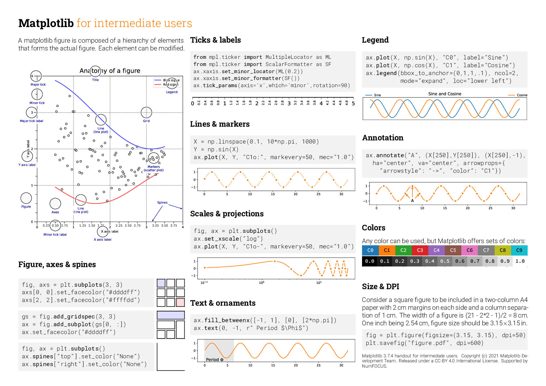
A matplotlib figure is composed of a hierarchy of elements that forms
the actual figure. Each element can be modified. \medskip
\includegraphics[width=\linewidth]{anatomy.pdf}
\subsection*{\rmfamily Figure, axes \& spines}
% -----------------------------------------------------------------------------
\begin{tabular}{@{}m{.821\linewidth}m{.169\linewidth}}
\begin{lstlisting}[belowskip=-\baselineskip]
fig, axs = plt.subplots(3, 3)
axs[0, 0].set_facecolor("#ddddff")
axs[2, 2].set_facecolor("#ffffdd")
\end{lstlisting}
& \raisebox{-0.75em}{\includegraphics[width=\linewidth]{layout-subplot-color.pdf}}
\end{tabular}
% -----------------------------------------------------------------------------
\begin{tabular}{@{}m{.821\linewidth}m{.169\linewidth}}
\begin{lstlisting}[belowskip=-\baselineskip]
gs = fig.add_gridspec(3, 3)
ax = fig.add_subplot(gs[0, :])
ax.set_facecolor("#ddddff")
\end{lstlisting}
& \raisebox{-0.75em}{\includegraphics[width=\linewidth]{layout-gridspec-color.pdf}}
\end{tabular}
% -----------------------------------------------------------------------------
\begin{tabular}{@{}m{.821\linewidth}m{.169\linewidth}}
\begin{lstlisting}[belowskip=-\baselineskip]
fig, ax = plt.subplots()
ax.spines["top"].set_color("None")
ax.spines["right"].set_color("None")
\end{lstlisting}
& \raisebox{-0.75em}{\includegraphics[width=\linewidth]{layout-spines.pdf}}
\end{tabular}
% -----------------------------------------------------------------------------
\subsection*{\rmfamily Ticks \& labels}
\begin{lstlisting}[basicstyle=\ttfamily\small]
from mpl.ticker import MultipleLocator as ML
from mpl.ticker import ScalarFormatter as SF
ax.xaxis.set_minor_locator(ML(0.2))
ax.xaxis.set_minor_formatter(SF())
ax.tick_params(axis='x',which='minor',rotation=90)
\end{lstlisting}
\includegraphics[width=\linewidth]{tick-multiple-locator.pdf}
% -----------------------------------------------------------------------------
\subsection*{\rmfamily Lines \& markers}
\begin{lstlisting}
X = np.linspace(0.1, 10*np.pi, 1000)
Y = np.sin(X)
ax.plot(X, Y, "C1o:", markevery=50, mec="1.0")
\end{lstlisting}
\includegraphics[width=\linewidth]{sine-marker.pdf}
% -----------------------------------------------------------------------------
\subsection*{\rmfamily Scales \& projections}
\begin{lstlisting}
fig, ax = plt.subplots()
ax.set_xscale("log")
ax.plot(X, Y, "C1o-", markevery=50, mec="1.0")
\end{lstlisting}
\includegraphics[width=\linewidth]{sine-logscale.pdf}
\subsection*{\rmfamily Text \& ornaments}
\begin{lstlisting}[]
ax.fill_betweenx([-1, 1], [0], [2*np.pi])
ax.text(0, -1, r" Period $\Phi$")
\end{lstlisting}
\includegraphics[width=\linewidth]{sine-period.pdf}
% -----------------------------------------------------------------------------
\subsection*{\rmfamily Legend}
\begin{lstlisting}[]
ax.plot(X, np.sin(X), "C0", label="Sine")
ax.plot(X, np.cos(X), "C1", label="Cosine")
ax.legend(bbox_to_anchor=(0,1,1,.1), ncol=2,
mode="expand", loc="lower left")
\end{lstlisting}
\includegraphics[width=\linewidth]{sine-legend.pdf}
% -----------------------------------------------------------------------------
\subsection*{\rmfamily Annotation}
\begin{lstlisting}[]
ax.annotate("A", (X[250],Y[250]), (X[250],-1),
ha="center", va="center", arrowprops={
"arrowstyle": "->", "color": "C1"})
\end{lstlisting}
\includegraphics[width=\linewidth]{sine-annotate.pdf}
% -----------------------------------------------------------------------------
\subsection*{\rmfamily Colors}
Any color can be used, but Matplotlib offers sets of colors:\\
\includegraphics[width=\linewidth]{colors-cycle.pdf} \smallskip
\includegraphics[width=\linewidth]{colors-grey.pdf}\\
%As well as nice colormaps (viridis an magma):\\
%\includegraphics[width=\linewidth]{colormap-viridis.pdf} \smallskip
%\includegraphics[width=\linewidth]{colormap-magma.pdf} \medskip
% -----------------------------------------------------------------------------
\vspace{-1em}
\subsection*{\rmfamily Size \& DPI}
Consider a square figure to be included in a two-column A4 paper with
2\,cm margins on each side and a column separation of 1\,cm. The width of
a figure is (21 - 2*2 - 1)/2 = 8\,cm. One inch being 2.54\,cm, figure size
should be 3.15$\times$3.15\,in.
\begin{lstlisting}[]
fig = plt.figure(figsize=(3.15, 3.15), dpi=50)
plt.savefig("figure.pdf", dpi=600)
\end{lstlisting}
\vfill
%
{\scriptsize
Matplotlib 3.9.4 handout for intermediate users.
Copyright (c) 2021 Matplotlib Development Team.
Released under a CC-BY 4.0 International License.
Supported by NumFOCUS.
\par}
\end{multicols*}
\end{document}
================================================
FILE: handout-tips.tex
================================================
\documentclass[10pt,landscape,a4paper]{article}
\usepackage[right=10mm, left=10mm, top=10mm, bottom=10mm]{geometry}
\usepackage[utf8]{inputenc}
\usepackage[T1]{fontenc}
\usepackage[english]{babel}
\usepackage[rm,light]{roboto}
\usepackage{xcolor}
\usepackage{graphicx}
\graphicspath{{./figures/}}
\usepackage{multicol}
\usepackage{colortbl}
\usepackage{array}
\setlength\parindent{0pt}
\setlength{\tabcolsep}{2pt}
\baselineskip=0pt
\setlength\columnsep{1em}
\definecolor{Gray}{gray}{0.85}
% --- Listing -----------------------------------------------------------------
\usepackage{listings}
\lstset{
frame=tb, framesep=4pt, framerule=0pt,
backgroundcolor=\color{black!5},
basicstyle=\ttfamily\footnotesize,
commentstyle=\ttfamily\color{black!50},
breakatwhitespace=false,
breaklines=true,
extendedchars=true,
keepspaces=true,
language=Python,
rulecolor=\color{black},
showspaces=false,
showstringspaces=false,
showtabs=false,
tabsize=2,
%
emph = {
plot, scatter, imshow, bar, contourf, pie, subplots, spines,
add_gridspec, add_subplot, set_xscale, set_minor_locator, linestyle,
dash_capstyle, projection, Stroke, Normal, add_axes, label, savefig,
get_cmap, histtype, annotate, set_minor_formatter, tick_params,
fill_betweenx, text, legend, errorbar, boxplot, hist, title, xlabel,
ylabel, suptitle, fraction, pad, set_fontname, get_xticklabels},
emphstyle = {\ttfamily\bfseries}
}
% --- Fonts -------------------------------------------------------------------
\usepackage{fontspec}
\usepackage[babel=true]{microtype}
\defaultfontfeatures{Ligatures = TeX, Mapping = tex-text}
\setsansfont{Roboto} [ Path = fonts/roboto/Roboto-,
Extension = .ttf,
UprightFont = Light,
ItalicFont = LightItalic,
BoldFont = Regular,
BoldItalicFont = Italic ]
\setromanfont{RobotoSlab} [ Path = fonts/roboto-slab/RobotoSlab-,
Extension = .ttf,
UprightFont = Light,
BoldFont = Bold ]
\setmonofont{RobotoMono} [ Path = fonts/roboto-mono/RobotoMono-,
Extension = .ttf,
Scale = 0.90,
UprightFont = Light,
ItalicFont = LightItalic,
BoldFont = Regular,
BoldItalicFont = Italic ]
\renewcommand{\familydefault}{\sfdefault}
% -----------------------------------------------------------------------------
\begin{document}
\thispagestyle{empty}
\section*{\LARGE \rmfamily
Matplotlib \textcolor{orange}{\mdseries tips \& tricks}}
\begin{multicols*}{3}
% -----------------------------------------------------------------------------
\subsection*{\rmfamily Transparency}
Scatter plots can be enhanced by using transparency (alpha) in order
to show area with higher density. Multiple scatter plots can be
used to delineate a frontier.
\begin{tabular}{@{}m{.774\linewidth}m{.216\linewidth}}
\begin{lstlisting}[belowskip=-\baselineskip]
X = np.random.normal(-1, 1, 500)
Y = np.random.normal(-1, 1, 500)
ax.scatter(X, Y, 50, "0.0", lw=2) # optional
ax.scatter(X, Y, 50, "1.0", lw=0) # optional
ax.scatter(X, Y, 40, "C1", lw=0, alpha=0.1)
\end{lstlisting} &
\raisebox{-0.75em}{\includegraphics[width=\linewidth]{tip-transparency.pdf}}
\end{tabular}
% -----------------------------------------------------------------------------
\subsection*{\rmfamily Rasterization}
If your figure has many graphical elements, such as a huge
scatter, you can rasterize them to save memory and keep other elements
in vector format.
\begin{lstlisting}
X = np.random.normal(-1, 1, 10_000)
Y = np.random.normal(-1, 1, 10_000)
ax.scatter(X, Y, rasterized=True)
fig.savefig("rasterized-figure.pdf", dpi=600)
\end{lstlisting}
% -----------------------------------------------------------------------------
\subsection*{\rmfamily Offline rendering}
Use the Agg backend to render a figure directly in an array.
\begin{lstlisting}
from matplotlib.backends.backend_agg import FigureCanvas
canvas = FigureCanvas(Figure()))
... # draw some stuff
canvas.draw()
Z = np.array(canvas.renderer.buffer_rgba())
\end{lstlisting}
% -----------------------------------------------------------------------------
\subsection*{\rmfamily Range of continuous colors}
You can use colormap to pick from a range of continuous colors.
\begin{tabular}{@{}m{.774\linewidth}m{.216\linewidth}}
\begin{lstlisting}[belowskip=-\baselineskip]
X = np.random.randn(1000, 4)
cmap = plt.get_cmap("Oranges")
colors = cmap([0.2, 0.4, 0.6, 0.8])
ax.hist(X, 2, histtype='bar', color=colors)
\end{lstlisting} &
\raisebox{-0.75em}{\includegraphics[width=\linewidth]{tip-color-range.pdf}}
\end{tabular}
% -----------------------------------------------------------------------------
\subsection*{\rmfamily Text outline}
Use text outline to make text more visible.
\begin{tabular}{@{}m{.774\linewidth}m{.216\linewidth}}
\begin{lstlisting}[belowskip=-\baselineskip]
import matplotlib.patheffects as fx
text = ax.text(0.5, 0.1, "Label")
text.set_path_effects([
fx.Stroke(linewidth=3, foreground='1.0'),
fx.Normal()])
\end{lstlisting} &
\raisebox{-0.75em}{\includegraphics[width=\linewidth]{tip-outline.pdf}}
\end{tabular}
% -----------------------------------------------------------------------------
\subsection*{\rmfamily Multiline plot}
You can plot several lines at once using {\em None} as separator.
\begin{lstlisting}
X,Y = [], []
for x in np.linspace(0, 10*np.pi, 100):
X.extend([x, x, None]), Y.extend([0, sin(x), None])
ax.plot(X, Y, "black")
\end{lstlisting}
\includegraphics[width=\linewidth]{tip-multiline.pdf}
% -----------------------------------------------------------------------------
\subsection*{\rmfamily Dotted lines}
To have rounded dotted lines, use a custom {\ttfamily linestyle} and
modify {\ttfamily dash\_capstyle}.
\begin{lstlisting}
ax.plot([0, 1], [0, 0], "C1",
linestyle=(0, (0.01, 1)), dash_capstyle="round")
ax.plot([0, 1], [1, 1], "C1",
linestyle=(0, (0.01, 2)), dash_capstyle="round")
\end{lstlisting}
\includegraphics[width=\linewidth]{tip-dotted.pdf}
% -----------------------------------------------------------------------------
\subsection*{\rmfamily Combining axes}
You can use overlaid axes with different projections.
\begin{tabular}{@{}m{.774\linewidth}m{.216\linewidth}}
\begin{lstlisting}[belowskip=-\baselineskip]
ax1 = fig.add_axes([0, 0, 1, 1],
label="cartesian")
ax2 = fig.add_axes([0, 0, 1, 1],
label="polar",
projection="polar")
\end{lstlisting} &
\raisebox{-0.75em}{\includegraphics[width=\linewidth]{tip-dual-axis.pdf}}
\end{tabular}
\subsection*{\rmfamily Colorbar adjustment}
You can adjust a colorbar's size when adding it.
\begin{tabular}{@{}m{.754\linewidth}m{.236\linewidth}}
\begin{lstlisting}[belowskip=-\baselineskip]
im = ax.imshow(Z)
cb = plt.colorbar(im,
fraction=0.046, pad=0.04)
cb.set_ticks([])
\end{lstlisting} &
\raisebox{-0.75em}{\includegraphics[width=\linewidth]{tip-colorbar.pdf}}
\end{tabular}
\subsection*{\rmfamily Taking advantage of typography}
You can use a condensed font such as Roboto
Condensed to save space on tick labels.
\begin{lstlisting}
for tick in ax.get_xticklabels(which='both'):
tick.set_fontname("Roboto Condensed")
\end{lstlisting}
\includegraphics[width=\linewidth]{tip-font-family.pdf}
\subsection*{\rmfamily Getting rid of margins}
Once your figure is finished, you can call {\ttfamily tight\_layout()}
to remove white margins. If there are remaining margins, you can use
the {\ttfamily pdfcrop} utility (comes with TeX live).
\subsection*{\rmfamily Hatching}
You can achieve a nice visual effect with thick hatch patterns.
\begin{tabular}{@{}m{.774\linewidth}m{.216\linewidth}}
\begin{lstlisting}[belowskip=-\baselineskip]
cmap = plt.get_cmap("Oranges")
plt.rcParams['hatch.color'] = cmap(0.2)
plt.rcParams['hatch.linewidth'] = 8
ax.bar(X, Y, color=cmap(0.6), hatch="/")
\end{lstlisting} &
\raisebox{-0.75em}{\includegraphics[width=\linewidth]{tip-hatched.pdf}}
\end{tabular}
\subsection*{\rmfamily Read the documentation}
Matplotlib comes with an extensive documentation explaining the
details of each command and is generally accompanied by examples.
Together with the huge online gallery, this documentation is a
gold-mine.
\vfill
%
{\scriptsize
Matplotlib 3.9.4 handout for tips \& tricks.
Copyright (c) 2021 Matplotlib Development Team.
Released under a CC-BY 4.0 International License.
Supported by NumFOCUS.
\par}
\end{multicols*}
\end{document}
================================================
FILE: logos/mpl-logos2.py
================================================
"""
===============
Matplotlib logo
===============
This example generates the current matplotlib logo.
"""
import numpy as np
import matplotlib.pyplot as plt
import matplotlib.cm as cm
import matplotlib.font_manager
from matplotlib.patches import Rectangle, PathPatch
from matplotlib.textpath import TextPath
import matplotlib.transforms as mtrans
MPL_BLUE = '#11557c'
def get_font_properties():
# The original font is Calibri, if that is not installed, we fall back
# to Carlito, which is metrically equivalent.
if 'Calibri' in matplotlib.font_manager.findfont('Calibri:bold'):
return matplotlib.font_manager.FontProperties(family='Calibri',
weight='bold')
if 'Carlito' in matplotlib.font_manager.findfont('Carlito:bold'):
print('Original font not found. Falling back to Carlito. '
'The logo text will not be in the correct font.')
return matplotlib.font_manager.FontProperties(family='Carlito',
weight='bold')
print('Original font not found. '
'The logo text will not be in the correct font.')
return None
def create_icon_axes(fig, ax_position, lw_bars, lw_grid, lw_border, rgrid):
"""
Create a polar axes containing the matplotlib radar plot.
Parameters
----------
fig : matplotlib.figure.Figure
The figure to draw into.
ax_position : (float, float, float, float)
The position of the created Axes in figure coordinates as
(x, y, width, height).
lw_bars : float
The linewidth of the bars.
lw_grid : float
The linewidth of the grid.
lw_border : float
The linewidth of the Axes border.
rgrid : array-like
Positions of the radial grid.
Returns
-------
ax : matplotlib.axes.Axes
The created Axes.
"""
with plt.rc_context({'axes.edgecolor': MPL_BLUE,
'axes.linewidth': lw_border}):
ax = fig.add_axes(ax_position, projection='polar')
ax.set_axisbelow(True)
N = 7
arc = 2. * np.pi
theta = np.arange(0.0, arc, arc / N)
radii = np.array([2, 6, 8, 7, 4, 5, 8])
width = np.pi / 4 * np.array([0.4, 0.4, 0.6, 0.8, 0.2, 0.5, 0.3])
bars = ax.bar(theta, radii, width=width, bottom=0.0, align='edge',
edgecolor='0.3', lw=lw_bars)
for r, bar in zip(radii, bars):
color = *cm.jet(r / 10.)[:3], 0.6 # color from jet with alpha=0.6
bar.set_facecolor(color)
ax.tick_params(labelbottom=False, labeltop=False,
labelleft=False, labelright=False)
ax.grid(lw=lw_grid, color='0.9')
ax.set_rmax(9)
ax.set_yticks(rgrid)
# the actual visible background - extends a bit beyond the axis
ax.add_patch(Rectangle((0, 0), arc, 9.58,
facecolor='white', zorder=0,
clip_on=False, in_layout=False))
return ax
def create_text_axes(fig, height_px):
"""Create an axes in *fig* that contains 'matplotlib' as Text."""
ax = fig.add_axes((0, 0, 1, 1))
ax.set_aspect("equal")
ax.set_axis_off()
path = TextPath((0, 0), "matplotlib", size=height_px * 0.8,
prop=get_font_properties())
fp = get_font_properties()
fp.set_weight('light')
path1 = TextPath((80, -13), 'Cheat sheet', size=height_px * 0.12,
prop=fp)
path2 = TextPath((310, -13), f'Version {matplotlib. __version__}',
size=height_px * 0.12,
prop=fp)
angle = 4.25 # degrees
trans = mtrans.Affine2D().skew_deg(angle, 0)
patch = PathPatch(path, transform=trans + ax.transData, color=MPL_BLUE,
lw=0)
patch1 = PathPatch(path1, transform=trans + ax.transData, color=MPL_BLUE,
lw=0)
patch2 = PathPatch(path2, color=MPL_BLUE,
lw=0)
ax.add_patch(patch)
ax.add_patch(patch1)
ax.add_patch(patch2)
ax.autoscale()
def make_logo(height_px, lw_bars, lw_grid, lw_border, rgrid, with_text=False):
"""
Create a full figure with the Matplotlib logo.
Parameters
----------
height_px : int
Height of the figure in pixel.
lw_bars : float
The linewidth of the bar border.
lw_grid : float
The linewidth of the grid.
lw_border : float
The linewidth of icon border.
rgrid : sequence of float
The radial grid positions.
with_text : bool
Whether to draw only the icon or to include 'matplotlib' as text.
"""
dpi = 100
height = height_px / dpi
figsize = (5 * height, height) if with_text else (height, height)
fig = plt.figure(figsize=figsize, dpi=dpi)
fig.patch.set_alpha(0)
if with_text:
create_text_axes(fig, height_px)
ax_pos = (0.535, 0.12, .17, 0.75) if with_text else (0.03, 0.03, .94, .94)
ax = create_icon_axes(fig, ax_pos, lw_bars, lw_grid, lw_border, rgrid)
fig.savefig('mpl-logo2.pdf')
return fig, ax
##############################################################################
# A large logo:
make_logo(height_px=110, lw_bars=0.7, lw_grid=0.5, lw_border=1,
rgrid=[1, 3, 5, 7])
##############################################################################
# A small 32px logo:
make_logo(height_px=32, lw_bars=0.3, lw_grid=0.3, lw_border=0.3, rgrid=[5])
##############################################################################
# A large logo including text, as used on the matplotlib website.
make_logo(height_px=110, lw_bars=0.7, lw_grid=0.5, lw_border=1,
rgrid=[1, 3, 5, 7], with_text=True)
# plt.show()
================================================
FILE: requirements/Makefile
================================================
.PHONY: default
default: all
.PHONY: all
all: requirements.txt
.PHONY: install
install: requirements.txt
pip-sync $^
%.txt: %.in
pip-compile $<
================================================
FILE: requirements/requirements.in
================================================
autopep8
bump2version
cartopy==0.22.0
flake8
matplotlib==3.9.4
pillow>=9
pdfx
pip-tools
pre-commit
scipy
# Docs
mpl-sphinx-theme~=3.9.0
pydata-sphinx-theme==0.13.3
sphinx
sphinx-design
================================================
FILE: requirements/requirements.txt
================================================
#
# This file is autogenerated by pip-compile with Python 3.10
# by the following command:
#
# pip-compile requirements.in
#
accessible-pygments==0.0.4
# via pydata-sphinx-theme
alabaster==0.7.16
# via sphinx
autopep8==2.0.4
# via -r requirements.in
babel==2.14.0
# via
# pydata-sphinx-theme
# sphinx
beautifulsoup4==4.12.3
# via pydata-sphinx-theme
build==1.0.3
# via pip-tools
bump2version==1.0.1
# via -r requirements.in
cartopy==0.22.0
# via -r requirements.in
certifi==2024.7.4
# via
# pyproj
# requests
cffi==1.16.0
# via cryptography
cfgv==3.4.0
# via pre-commit
chardet==4.0.0
# via
# pdfminer-six
# pdfx
charset-normalizer==3.3.2
# via requests
click==8.1.7
# via pip-tools
contourpy==1.2.0
# via matplotlib
cryptography==44.0.1
# via pdfminer-six
cycler==0.12.1
# via matplotlib
distlib==0.3.8
# via virtualenv
docutils==0.20.1
# via
# pydata-sphinx-theme
# sphinx
filelock==3.13.1
# via virtualenv
flake8==7.0.0
# via -r requirements.in
fonttools==4.47.2
# via matplotlib
identify==2.5.33
# via pre-commit
idna==3.7
# via requests
imagesize==1.4.1
# via sphinx
jinja2==3.1.5
# via sphinx
kiwisolver==1.4.5
# via matplotlib
markupsafe==2.1.4
# via jinja2
matplotlib==3.9.4
# via
# -r requirements.in
# cartopy
# mpl-sphinx-theme
mccabe==0.7.0
# via flake8
mpl-sphinx-theme==3.9.0
# via -r requirements.in
nodeenv==1.8.0
# via pre-commit
numpy==1.26.3
# via
# cartopy
# contourpy
# matplotlib
# scipy
# shapely
packaging==23.2
# via
# build
# cartopy
# matplotlib
# pydata-sphinx-theme
# sphinx
pdfminer-six==20201018
# via pdfx
pdfx==1.4.1
# via -r requirements.in
pillow==10.3.0
# via
# -r requirements.in
# matplotlib
pip-tools==7.3.0
# via -r requirements.in
platformdirs==4.2.0
# via virtualenv
pre-commit==3.6.0
# via -r requirements.in
pycodestyle==2.11.1
# via
# autopep8
# flake8
pycparser==2.21
# via cffi
pydata-sphinx-theme==0.13.3
# via
# -r requirements.in
# mpl-sphinx-theme
pyflakes==3.2.0
# via flake8
pygments==2.17.2
# via
# accessible-pygments
# pydata-sphinx-theme
# sphinx
pyparsing==3.1.1
# via matplotlib
pyproj==3.6.1
# via cartopy
pyproject-hooks==1.0.0
# via build
pyshp==2.3.1
# via cartopy
python-dateutil==2.8.2
# via matplotlib
pyyaml==6.0.1
# via pre-commit
requests==2.32.4
# via sphinx
scipy==1.12.0
# via -r requirements.in
shapely==2.0.2
# via cartopy
six==1.16.0
# via python-dateutil
snowballstemmer==2.2.0
# via sphinx
sortedcontainers==2.4.0
# via pdfminer-six
soupsieve==2.5
# via beautifulsoup4
sphinx==7.2.6
# via
# -r requirements.in
# pydata-sphinx-theme
# sphinx-design
sphinx-design==0.5.0
# via -r requirements.in
sphinxcontrib-applehelp==1.0.8
# via sphinx
sphinxcontrib-devhelp==1.0.6
# via sphinx
sphinxcontrib-htmlhelp==2.0.5
# via sphinx
sphinxcontrib-jsmath==1.0.1
# via sphinx
sphinxcontrib-qthelp==1.0.7
# via sphinx
sphinxcontrib-serializinghtml==1.1.10
# via sphinx
tomli==2.0.1
# via
# autopep8
# build
# pip-tools
# pyproject-hooks
typing-extensions==4.9.0
# via pydata-sphinx-theme
urllib3==2.5.0
# via requests
virtualenv==20.26.6
# via pre-commit
wheel==0.42.0
# via pip-tools
# The following packages are considered to be unsafe in a requirements file:
# pip
# setuptools
================================================
FILE: scripts/adjustements.py
================================================
# -----------------------------------------------------------------------------
# Matplotlib cheat sheet
# Released under the BSD License
# -----------------------------------------------------------------------------
import pathlib
import numpy as np
import matplotlib as mpl
import matplotlib.pyplot as plt
import matplotlib.patches as mpatches
from matplotlib.collections import PatchCollection
ROOT_DIR = pathlib.Path(__file__).parent.parent
mpl.style.use([
ROOT_DIR / 'styles/base.mplstyle',
])
mpl.rc('font', size=4)
mpl.rc('lines', linewidth=0.5)
mpl.rc('patch', linewidth=0.5)
subplots_kw = dict(
figsize=(5.7/2.54, 5.7/2.54 * 95/115),
subplot_kw=dict(
frameon=False,
aspect=1,
xlim=(0-5, 100+10),
ylim=(-10, 80+5),
xticks=[],
yticks=[],
),
)
(fig, ax) = plt.subplots(**subplots_kw)
box = mpatches.FancyBboxPatch(
(0, 0), 100, 83, mpatches.BoxStyle("Round", pad=0, rounding_size=2),
facecolor="0.9", edgecolor="black")
ax.add_artist(box)
box = mpatches.FancyBboxPatch(
(0, 0), 100, 75, mpatches.BoxStyle("Round", pad=0, rounding_size=0),
facecolor="white", edgecolor="black")
ax.add_artist(box)
box = mpatches.Rectangle(
(5, 5), 45, 30, zorder=10,
facecolor="white", edgecolor="black")
ax.add_artist(box)
box = mpatches.Rectangle(
(5, 40), 45, 30, zorder=10,
facecolor="white", edgecolor="black")
ax.add_artist(box)
box = mpatches.Rectangle(
(55, 5), 40, 65, zorder=10,
facecolor="white", edgecolor="black")
ax.add_artist(box)
# Window button
X, Y = [5, 10, 15], [79, 79, 79]
plt.scatter(X, Y, s=20, zorder=10,
edgecolor="black", facecolor="white")
# Window size extension
X, Y = [0, 0], [0, -8]
plt.plot(X, Y, color="black", linestyle=":", clip_on=False)
X, Y = [100, 100], [0, -8]
plt.plot(X, Y, color="black", linestyle=":", clip_on=False)
X, Y = [100, 108], [0, 0]
plt.plot(X, Y, color="black", linestyle=":", clip_on=False)
X, Y = [100, 108], [75, 75]
plt.plot(X, Y, color="black", linestyle=":", clip_on=False)
def ext_arrow(p0, p1, p2, p3):
p0, p1 = np.asarray(p0), np.asarray(p1)
p2, p3 = np.asarray(p2), np.asarray(p3)
ax.arrow(*p0, *(p1-p0), zorder=20, linewidth=0,
length_includes_head=True, width=.4,
head_width=2, head_length=2, color="black")
ax.arrow(*p3, *(p2-p3), zorder=20, linewidth=0,
length_includes_head=True, width=.4,
head_width=2, head_length=2, color="black")
plt.plot([p1[0], p2[0]], [p1[1], p2[1]], linewidth=.5, color="black")
def int_arrow(p0, p1):
p0, p1 = np.asarray(p0), np.asarray(p1)
ax.arrow(*((p0+p1)/2), *((p1-p0)/2), zorder=20, linewidth=0,
length_includes_head=True, width=.4,
head_width=2, head_length=2, color="black")
ax.arrow(*((p0+p1)/2), *(-(p1-p0)/2), zorder=20, linewidth=0,
length_includes_head=True, width=.4,
head_width=2, head_length=2, color="black")
x = 0
y = 10
ext_arrow( (x-4, y), (x, y), (x+5, y), (x+9, y) )
ax.text(x+9.5, y, "left", ha="left", va="center", zorder=20)
x += 50
ext_arrow( (x-4, y), (x, y), (x+5, y), (x+9, y) )
ax.text(x-4.5, y, "wspace", ha="right", va="center", zorder=20)
x += 45
ext_arrow( (x-4, y), (x, y), (x+5, y), (x+9, y) )
ax.text(x-4.5, y, "right", ha="right", va="center", zorder=20)
y = 0
x = 25
ext_arrow( (x, y-4), (x, y), (x, y+5), (x, y+9) )
ax.text(x, y+9.5, "bottom", ha="center", va="bottom", zorder=20)
y += 35
ext_arrow( (x, y-4), (x, y), (x, y+5), (x, y+9) )
ax.text(x, y-4.5, "hspace", ha="center", va="top", zorder=20)
y += 35
ext_arrow( (x, y-4), (x, y), (x, y+5), (x, y+9) )
ax.text(x, y-4.5, "top", ha="center", va="top", zorder=20)
int_arrow((0, -5), (100, -5))
ax.text(50, -5, "figure width", backgroundcolor="white", zorder=30,
ha="center", va="center")
int_arrow((105, 0), (105, 75))
ax.text(105, 75/2, "figure height", backgroundcolor="white", zorder=30,
rotation="vertical", ha="center", va="center")
int_arrow((55, 62.5), (95, 62.5))
ax.text(75, 62.5, "axes width", backgroundcolor="white", zorder=30,
ha="center", va="center")
int_arrow((62.5, 5), (62.5, 70))
ax.text(62.5, 35, "axes height", backgroundcolor="white", zorder=30,
rotation="vertical", ha="center", va="center")
fig.savefig(ROOT_DIR / "figures/adjustments.pdf")
================================================
FILE: scripts/advanced-plots.py
================================================
# -----------------------------------------------------------------------------
# Matplotlib cheat sheet
# Released under the BSD License
# -----------------------------------------------------------------------------
# Script to generate all the advanced plots
import pathlib
import numpy as np
import matplotlib as mpl
import matplotlib.pyplot as plt
ROOT_DIR = pathlib.Path(__file__).parent.parent
mpl.style.use([
ROOT_DIR / 'styles/base.mplstyle',
ROOT_DIR / 'styles/plotlet.mplstyle',
])
subplot_kw = dict(
xlim=(0, 8), xticks=np.arange(1, 8),
ylim=(0, 8), yticks=np.arange(1, 8),
)
# Step plot
# -----------------------------------------------------------------------------
(fig, ax) = plt.subplots(subplot_kw=subplot_kw)
X = np.linspace(0, 10, 16)
Y = 4 + 2*np.sin(2*X)
ax.step(X, Y, color="C1")
ax.grid()
fig.savefig(ROOT_DIR / "figures/advanced-step.pdf")
# Violin plot
# -----------------------------------------------------------------------------
(fig, ax) = plt.subplots(subplot_kw=subplot_kw)
np.random.seed(10)
D = np.random.normal((3, 5, 4), (0.75, 1.00, 0.75), (200, 3))
VP = ax.violinplot(D, [2, 4, 6], widths=1.5,
showmeans=False, showmedians=False, showextrema=False)
for body in VP['bodies']:
body.set_facecolor('C1')
body.set_alpha(1)
ax.set_axisbelow(True)
ax.grid()
fig.savefig(ROOT_DIR / "figures/advanced-violin.pdf")
# Boxplot
# -----------------------------------------------------------------------------
(fig, ax) = plt.subplots(subplot_kw=subplot_kw)
np.random.seed(10)
D = np.random.normal((3, 5, 4), (1.25, 1.00, 1.25), (100, 3))
VP = ax.boxplot(D, positions=[2, 4, 6], widths=1.5, patch_artist=True,
showmeans=False, showfliers=False,
medianprops={"color": "white",
"linewidth": 0.25},
boxprops={"facecolor": "C1",
"edgecolor": "white",
"linewidth": 0.25},
whiskerprops={"color": "C1",
"linewidth": 0.75},
capprops={"color": "C1",
"linewidth": 0.75})
ax.set_axisbelow(True)
ax.grid()
fig.savefig(ROOT_DIR / "figures/advanced-boxplot.pdf")
# Barbs plot
# -----------------------------------------------------------------------------
(fig, ax) = plt.subplots(subplot_kw=subplot_kw)
np.random.seed(1)
X = [[2, 4, 6]]
Y = [[1.5, 3, 2]]
U = -np.ones((1, 3)) * 0
V = -np.ones((1, 3)) * np.linspace(50, 100, 3)
ax.barbs(X, Y, U, V, barbcolor="C1", flagcolor="C1", length=5, linewidth=0.5)
ax.set_axisbelow(True)
ax.grid()
fig.savefig(ROOT_DIR / "figures/advanced-barbs.pdf")
# Event plot
# -----------------------------------------------------------------------------
(fig, ax) = plt.subplots(subplot_kw=subplot_kw)
np.random.seed(1)
X = [2, 4, 6]
D = np.random.gamma(4, size=(3, 50))
ax.eventplot(D, colors="C1", orientation="vertical", lineoffsets=X,
linewidth=0.25)
ax.set_axisbelow(True)
ax.grid()
fig.savefig(ROOT_DIR / "figures/advanced-event.pdf")
# Errorbar plot
# -----------------------------------------------------------------------------
(fig, ax) = plt.subplots(subplot_kw=subplot_kw)
np.random.seed(1)
X = [2, 4, 6]
Y = [4, 5, 4]
E = np.random.uniform(0.5, 1.5, 3)
ax.errorbar(X, Y, E, color="C1", linewidth=0.75, capsize=1)
ax.set_axisbelow(True)
ax.grid()
fig.savefig(ROOT_DIR / "figures/advanced-errorbar.pdf")
# Hexbin plot
# -----------------------------------------------------------------------------
(fig, ax) = plt.subplots(subplot_kw=subplot_kw)
np.random.seed(1)
X = np.random.uniform(1.5, 6.5, 100)
Y = np.random.uniform(1.5, 6.5, 100)
C = np.random.uniform(0, 1, 10000)
ax.hexbin(X, Y, C, gridsize=4, linewidth=0.25, edgecolor="white",
cmap=plt.get_cmap("Wistia"), alpha=1.0)
ax.set_axisbelow(True)
ax.grid()
fig.savefig(ROOT_DIR / "figures/advanced-hexbin.pdf")
# Hist plot
# -----------------------------------------------------------------------------
(fig, ax) = plt.subplots(subplot_kw=subplot_kw)
np.random.seed(1)
X = 4 + np.random.normal(0, 1.5, 200)
ax.hist(X, bins=8, facecolor="C1", linewidth=0.25, edgecolor="white")
ax.set_ylim(0, 80), ax.set_yticks(np.arange(1, 80, 10))
ax.set_axisbelow(True)
ax.grid()
fig.savefig(ROOT_DIR / "figures/advanced-hist.pdf")
# Xcorr plot
# -----------------------------------------------------------------------------
(fig, ax) = plt.subplots(subplot_kw=subplot_kw)
np.random.seed(3)
Y = np.random.uniform(-4, 4, 250)
X = np.random.uniform(-4, 4, 250)
ax.xcorr(X, Y, usevlines=True, maxlags=6, normed=True, lw=1,
color="C1")
ax.set_xlim(-8, 8), ax.set_xticks(np.arange(-8, 8, 2))
ax.set_ylim(-.25, .25), ax.set_yticks(np.linspace(-.25, .25, 9))
ax.set_axisbelow(True)
ax.grid()
fig.savefig(ROOT_DIR / "figures/advanced-xcorr.pdf")
================================================
FILE: scripts/anatomy.py
================================================
# ----------------------------------------------------------------------------
# Title: Scientific Visualisation - Python & Matplotlib
# Author: Nicolas P. Rougier
# License: BSD
# ----------------------------------------------------------------------------
import pathlib
import numpy as np
import matplotlib as mpl
import matplotlib.pyplot as plt
from matplotlib.ticker import AutoMinorLocator, MultipleLocator, FuncFormatter
ROOT_DIR = pathlib.Path(__file__).parent.parent
mpl.style.use([
ROOT_DIR / 'styles/base.mplstyle',
])
np.random.seed(123)
X = np.linspace(0.5, 3.5, 100)
Y1 = 3+np.cos(X)
Y2 = 1+np.cos(1+X/0.75)/2
Y3 = np.random.uniform(Y1, Y2, len(X))
(fig, ax) = plt.subplots(figsize=(8, 8), subplot_kw=dict(aspect=1))
def minor_tick(x, pos):
if not x % 1.0:
return ""
return "%.2f" % x
ax.xaxis.set_major_locator(MultipleLocator(1.000))
ax.xaxis.set_minor_locator(AutoMinorLocator(4))
ax.yaxis.set_major_locator(MultipleLocator(1.000))
ax.yaxis.set_minor_locator(AutoMinorLocator(4))
ax.xaxis.set_minor_formatter(FuncFormatter(minor_tick))
ax.set_xlim(0, 4)
ax.set_ylim(0, 4)
ax.tick_params(which='major', width=1.0)
ax.tick_params(which='major', length=10)
ax.tick_params(which='minor', width=1.0, labelsize=10)
ax.tick_params(which='minor', length=5, labelsize=10, labelcolor='0.25')
ax.grid(linestyle="--", linewidth=0.5, color='.25', zorder=-10)
ax.plot(X, Y1, c=(0.25, 0.25, 1.00), lw=2, label="Blue signal", zorder=10)
ax.plot(X, Y2, c=(1.00, 0.25, 0.25), lw=2, label="Red signal")
ax.plot(X, Y3, linewidth=0,
marker='o', markerfacecolor='w', markeredgecolor='k')
ax.set_title("Anatomy of a figure", fontsize=20, verticalalignment='bottom')
ax.set_xlabel("X axis label")
ax.set_ylabel("Y axis label")
ax.legend(loc="upper right")
def circle(x, y, radius=0.15):
from matplotlib.patches import Circle
from matplotlib.patheffects import withStroke
circle = Circle((x, y), radius, clip_on=False, zorder=10, linewidth=1,
edgecolor='black', facecolor=(0, 0, 0, .0125),
path_effects=[withStroke(linewidth=5, foreground='w')])
ax.add_artist(circle)
def text(x, y, text):
ax.text(x, y, text, backgroundcolor="white",
# fontname="Yanone Kaffeesatz", fontsize="large",
ha='center', va='top', weight="regular", color='#000099')
# Minor tick
circle(0.50, -0.10)
text(0.50, -0.32, "Minor tick label")
# Major tick
circle(-0.03, 4.00)
text(0.03, 3.80, "Major tick")
# Minor tick
circle(0.00, 3.50)
text(0.00, 3.30, "Minor tick")
# Major tick label
circle(-0.15, 3.00)
text(-0.15, 2.80, "Major tick label")
# X Label
circle(1.80, -0.27)
text(1.80, -0.45, "X axis label")
# Y Label
circle(-0.27, 1.80)
text(-0.27, 1.6, "Y axis label")
# Title
circle(1.60, 4.13)
text(1.60, 3.93, "Title")
# Blue plot
circle(1.75, 2.80)
text(1.75, 2.60, "Line\n(line plot)")
# Red plot
circle(1.20, 0.60)
text(1.20, 0.40, "Line\n(line plot)")
# Scatter plot
circle(3.20, 1.75)
text(3.20, 1.55, "Markers\n(scatter plot)")
# Grid
circle(3.00, 3.00)
text(3.00, 2.80, "Grid")
# Legend
circle(3.70, 3.80)
text(3.70, 3.60, "Legend")
# Axes
circle(0.5, 0.5)
text(0.5, 0.3, "Axes")
# Figure
circle(-0.3, 0.65)
text(-0.3, 0.45, "Figure")
color = '#000099'
ax.annotate('Spines', xy=(4.0, 0.35), xytext=(3.3, 0.5), color=color,
weight='regular', # fontsize="large", fontname="Yanone Kaffeesatz",
arrowprops=dict(arrowstyle='->',
connectionstyle="arc3",
color=color))
ax.annotate('', xy=(3.15, 0.0), xytext=(3.45, 0.45), color=color,
weight='regular', # fontsize="large", fontname="Yanone Kaffeesatz",
arrowprops=dict(arrowstyle='->',
connectionstyle="arc3",
color=color))
fig.savefig(ROOT_DIR / "figures/anatomy.pdf")
# plt.show()
================================================
FILE: scripts/animation.py
================================================
import numpy as np
import matplotlib.pyplot as plt
import matplotlib.animation as animation
T = np.linspace(0, 2*np.pi, 100)
S = np.sin(T)
line, = plt.plot(T, S)
def animate(i):
line.set_ydata(np.sin(T+i/50))
a=animation.FuncAnimation(
plt.gcf(), animate, interval=5)
# plt.show()
================================================
FILE: scripts/annotate.py
================================================
# -----------------------------------------------------------------------------
# Matplotlib cheat sheet
# Released under the BSD License
# -----------------------------------------------------------------------------
import pathlib
import numpy as np
import matplotlib as mpl
import matplotlib.pyplot as plt
ROOT_DIR = pathlib.Path(__file__).parent.parent
fig = plt.figure(figsize=(6, 1))
# ax = plt.subplot(111, frameon=False, aspect=.1)
# b = 0.0
ax = fig.add_axes([0, 0, 1, 1], frameon=False, aspect=1)
plt.scatter([5.5], [0.75], s=100, c="k")
plt.xlim(0, 6), plt.ylim(0, 1)
plt.xticks([]), plt.yticks([])
plt.annotate("text", (5.5, .75), (0.75, .75), size=16, va="center", ha="center",
arrowprops=dict(facecolor='black', shrink=0.05))
plt.text( 5.5, 0.6, "xy\nxycoords", size=10, va="top", ha="center", color=".5")
plt.text( .75, 0.6, "xytext\ntextcoords", size=10, va="top", ha="center", color=".5")
fig.savefig(ROOT_DIR / "figures/annotate.pdf")
# plt.show()
================================================
FILE: scripts/annotation-arrow-styles.py
================================================
import pathlib
import matplotlib.pyplot as plt
import matplotlib.patches as mpatches
ROOT_DIR = pathlib.Path(__file__).parent.parent
styles = mpatches.ArrowStyle.get_styles()
def demo_con_style(ax, connectionstyle):
ax.text(.05, .95, connectionstyle.replace(",", ",\n"),
family="Source Code Pro",
transform=ax.transAxes, ha="left", va="top", size="x-small")
(fig, axes) = plt.subplots(4, 4, figsize=(4, 2.5), frameon=False)
for ax in axes.flatten():
ax.axis("off")
for i, (ax, style) in enumerate(zip(axes.flatten(), mpatches.ArrowStyle.get_styles())):
x0, y0 = 0.8, 0.5
x1, y1 = 0.2, 0.5
ax.plot([x0, x1], [y0, y1], ".", color="0.25")
ax.annotate("",
xy=(x0, y0), xycoords='data',
xytext=(x1, y1), textcoords='data',
arrowprops=dict(arrowstyle=style,
color="black",
shrinkA=5, shrinkB=5,
patchA=None, patchB=None,
connectionstyle="arc3,rad=0"))
ax.text( (x1+x0)/2, y0-0.2, style,
transform=ax.transAxes,
family="Source Code Pro", ha="center", va="top")
fig.savefig(ROOT_DIR / "figures/annotation-arrow-styles.pdf")
# plt.show()
================================================
FILE: scripts/annotation-connection-styles.py
================================================
import pathlib
import matplotlib as mpl
import matplotlib.pyplot as plt
ROOT_DIR = pathlib.Path(__file__).parent.parent
mpl.style.use([
ROOT_DIR / 'styles/base.mplstyle',
ROOT_DIR / 'styles/plotlet-grid.mplstyle',
])
mpl.rc('lines', markersize=3)
def demo_con_style(ax, connectionstyle):
x1, y1 = 0.3, 0.2
x2, y2 = 0.8, 0.6
ax.plot([x1, x2], [y1, y2], ".")
ax.annotate("",
xy=(x1, y1), xycoords='data',
xytext=(x2, y2), textcoords='data',
arrowprops=dict(arrowstyle="->", lw=0.5, color="0.5",
shrinkA=3, shrinkB=3,
patchA=None, patchB=None,
connectionstyle=connectionstyle),
)
ax.text(.05, .95, connectionstyle.replace(",", ",\n"),
transform=ax.transAxes, ha="left", va="top", size=4)
fig, axs = plt.subplots(3, 3, figsize=(5.7/2.54, 5.7/2.54))
demo_con_style(axs[0, 0], "arc3,rad=0")
demo_con_style(axs[0, 1], "arc3,rad=0.3")
demo_con_style(axs[0, 2], "angle3,angleA=0,angleB=90")
demo_con_style(axs[1, 0], "angle,angleA=-90,angleB=180,rad=0")
demo_con_style(axs[1, 1], "angle,angleA=-90,angleB=180,rad=10")
demo_con_style(axs[1, 2], "arc,angleA=-90,angleB=0,armA=0,armB=20,rad=0")
demo_con_style(axs[2, 0], "bar,fraction=0.3")
demo_con_style(axs[2, 1], "bar,fraction=-0.3")
demo_con_style(axs[2, 2], "bar,angle=180,fraction=-0.2")
for ax in axs.flat:
ax.set(xlim=(0, 1), ylim=(0, 1), xticks=[], yticks=[], aspect=1)
fig.savefig(ROOT_DIR / "figures/annotation-connection-styles.pdf")
================================================
FILE: scripts/basic-plots.py
================================================
# -----------------------------------------------------------------------------
# Matplotlib cheat sheet
# Released under the BSD License
# -----------------------------------------------------------------------------
# Script to generate all the basic plots
import pathlib
import numpy as np
import matplotlib as mpl
import matplotlib.pyplot as plt
ROOT_DIR = pathlib.Path(__file__).parent.parent
mpl.style.use([
ROOT_DIR / 'styles/base.mplstyle',
ROOT_DIR / 'styles/plotlet.mplstyle',
])
subplot_kw = dict(
xlim=(0, 8), xticks=np.arange(1, 8),
ylim=(0, 8), yticks=np.arange(1, 8),
)
# Basic line plot
# -----------------------------------------------------------------------------
(fig, ax) = plt.subplots(subplot_kw=subplot_kw)
X = np.linspace(0, 10, 100)
Y = 4 + 2*np.sin(2*X)
ax.plot(X, Y, color="C1")
ax.grid()
fig.savefig(ROOT_DIR / "figures/basic-plot.pdf")
# Basic line plot (color)
# -----------------------------------------------------------------------------
(fig, ax) = plt.subplots(subplot_kw=subplot_kw)
X = np.linspace(0, 10, 100)
Y = 4 + 2*np.sin(2*X)
ax.plot(X, Y, color="black")
ax.grid()
fig.savefig(ROOT_DIR / "figures/basic-plot-color.pdf")
# Basic scatter plot
# -----------------------------------------------------------------------------
(fig, ax) = plt.subplots(subplot_kw=subplot_kw)
np.random.seed(3)
X = 4 + np.random.normal(0, 1.25, 24)
Y = 4 + np.random.normal(0, 1.25, len(X))
ax.scatter(X, Y, 5, zorder=10,
edgecolor="white", facecolor="C1", linewidth=0.25)
ax.grid()
fig.savefig(ROOT_DIR / "figures/basic-scatter.pdf")
# Basic bar plot
# -----------------------------------------------------------------------------
(fig, ax) = plt.subplots(subplot_kw=subplot_kw)
np.random.seed(3)
X = 0.5 + np.arange(8)
Y = np.random.uniform(2, 7, len(X))
ax.bar(X, Y, bottom=0, width=1,
edgecolor="white", facecolor="C1", linewidth=0.25)
ax.set_axisbelow(True)
ax.grid()
fig.savefig(ROOT_DIR / "figures/basic-bar.pdf")
# Basic imshow plot
# -----------------------------------------------------------------------------
(fig, ax) = plt.subplots(subplot_kw=subplot_kw)
np.random.seed(3)
Z = np.zeros((8, 8, 4))
Z[:, :] = mpl.colors.to_rgba("C1")
Z[..., 3] = np.random.uniform(0.25, 1.0, (8, 8))
ax.imshow(Z, extent=[0, 8, 0, 8], interpolation="nearest")
ax.grid(linewidth=0.25, color="white")
fig.savefig(ROOT_DIR / "figures/basic-imshow.pdf")
# Basic pcolormesh plot
# -----------------------------------------------------------------------------
(fig, ax) = plt.subplots(subplot_kw=subplot_kw)
np.random.seed(1)
X, Y = np.meshgrid(np.linspace(-3, 3, 256), np.linspace(-3, 3, 256))
Z = (1 - X/2. + X**5 + Y**3) * np.exp(-X**2 - Y**2)
Z = Z - Z.min()
plt.pcolormesh(X, Y, Z, cmap='Oranges', shading='auto')
ax.set_xlim(-3, 3), ax.set_xticks(np.arange(-3, 4))
ax.set_ylim(-3, 3), ax.set_yticks(np.arange(-3, 4))
fig.savefig(ROOT_DIR / "figures/basic-pcolormesh.pdf")
# Basic contour plot
# -----------------------------------------------------------------------------
(fig, ax) = plt.subplots(subplot_kw=subplot_kw)
colors = np.zeros((5, 4))
colors[:] = mpl.colors.to_rgba("C1")
colors[:, 3] = np.linspace(0.15, 0.85, len(colors))
plt.contourf(Z, len(colors), extent=[0, 8, 0, 8], colors=colors)
plt.contour(Z, len(colors), extent=[0, 8, 0, 8], colors="white",
linewidths=0.125, nchunk=10)
fig.savefig(ROOT_DIR / "figures/basic-contour.pdf")
# Basic pie plot
# -----------------------------------------------------------------------------
(fig, ax) = plt.subplots(subplot_kw=subplot_kw)
X = [1, 2, 3, 4]
colors = np.zeros((len(X), 4))
colors[:] = mpl.colors.to_rgba("C1")
colors[:, 3] = np.linspace(0.25, 0.75, len(X))
ax.set_axisbelow(True)
ax.grid(linewidth=0.25, color="0.75")
ax.pie(X, colors=["white"] * len(X), radius=3, center=(4, 4),
wedgeprops={"linewidth": 0.25, "edgecolor": "white"}, frame=True)
ax.pie(X, colors=colors, radius=3, center=(4, 4),
wedgeprops={"linewidth": 0.25, "edgecolor": "white"}, frame=True)
fig.savefig(ROOT_DIR / "figures/basic-pie.pdf")
# Basic text plot
# -----------------------------------------------------------------------------
(fig, ax) = plt.subplots(subplot_kw=subplot_kw)
ax.set_axisbelow(True)
ax.grid(linewidth=0.25, color="0.75")
ax.text(4, 4, "TEXT", color="C1", size=8, weight="bold",
ha="center", va="center", rotation=25)
fig.savefig(ROOT_DIR / "figures/basic-text.pdf")
# Basic fill plot
# -----------------------------------------------------------------------------
(fig, ax) = plt.subplots(subplot_kw=subplot_kw)
np.random.seed(1)
X = np.linspace(0, 8, 16)
Y1 = 3 + 4*X/8 + np.random.uniform(0.0, 0.5, len(X))
Y2 = 1 + 2*X/8 + np.random.uniform(0.0, 0.5, len(X))
plt.fill_between(X, Y1, Y2, color="C1", alpha=.5, linewidth=0)
plt.plot(X, (Y1+Y2)/2, color="C1", linewidth=0.5)
ax.set_axisbelow(True)
ax.grid(color="0.75")
fig.savefig(ROOT_DIR / "figures/basic-fill.pdf")
# Basic quiver plot
# -----------------------------------------------------------------------------
(fig, ax) = plt.subplots(subplot_kw=subplot_kw)
np.random.seed(1)
T = np.linspace(0, 2*np.pi, 8)
X, Y = 4 + np.cos(T), 4 + np.sin(T)
U, V = 1.5*np.cos(T), 1.5*np.sin(T)
plt.quiver(X, Y, U, V, color="C1",
angles='xy', scale_units='xy', scale=0.5, width=.05)
ax.set_axisbelow(True)
ax.grid(color="0.75")
fig.savefig(ROOT_DIR / "figures/basic-quiver.pdf")
================================================
FILE: scripts/colorbar.py
================================================
# -----------------------------------------------------------------------------
# Matplotlib cheat sheet
# Released under the BSD License
# -----------------------------------------------------------------------------
import pathlib
import numpy as np
import matplotlib as mpl
import matplotlib.pyplot as plt
ROOT_DIR = pathlib.Path(__file__).parent.parent
fig = plt.figure(figsize=(6, .65))
# ax = plt.subplot(111, frameon=False, aspect=.1)
b = 0.025
ax = fig.add_axes([b, 10*b, 1-2*b, 1-10*b], frameon=False, aspect=0.05)
cmap = plt.get_cmap("Oranges")
norm = mpl.colors.Normalize(vmin=0, vmax=1)
sm = plt.cm.ScalarMappable(cmap=cmap, norm=norm)
sm.set_array([])
plt.colorbar(sm, cax=ax, ticks=np.linspace(0, 1, 11),
orientation="horizontal")
fig.savefig(ROOT_DIR / "figures/colorbar.pdf")
# plt.show()
================================================
FILE: scripts/colormaps.py
================================================
import pathlib
import numpy as np
import matplotlib.pyplot as plt
ROOT_DIR = pathlib.Path(__file__).parent.parent
figsize = 4.0, 0.25
fig = plt.figure(figsize=figsize)
ax = fig.add_axes([0, 0, 1, 1], frameon=False, aspect=1)
ymin, ymax= 0, 1
xmin, xmax = 0, figsize[0]/figsize[1]
# Uniform colormaps
# -----------------------------------------------------------------------------
cmaps = ('viridis', 'plasma', 'inferno', 'magma', 'cividis',
'PRGn', 'PiYG', 'RdYlGn', 'BrBG', 'RdGy', 'PuOr', 'RdBu',
'RdYlBu', 'Spectral', 'coolwarm', 'bwr', 'seismic',
'tab10', 'tab20', 'tab20b', 'tab20c',
'Pastel1', 'Pastel2', 'Paired',
'Set1', 'Set2', 'Set3', 'Accent', 'Dark2',
'Greys', 'Reds', 'Oranges', 'YlOrBr', 'YlOrRd', 'OrRd',
'PuRd', 'RdPu', 'BuPu', 'Purples', 'YlGnBu', 'Blues',
'PuBu', 'GnBu', 'PuBuGn', 'BuGn', 'Greens', 'YlGn',
'bone', 'gray', 'pink', 'afmhot', 'hot', 'gist_heat', 'copper',
'Wistia', 'autumn', 'summer', 'spring', 'cool', 'winter',
'twilight', 'twilight_shifted', 'hsv',
'terrain', 'ocean', 'gist_earth', 'cubehelix', 'rainbow'
)
for name in cmaps:
# The maximum number of segments in a cmap is 256, and for anything smaller,
# the cmap will map as a suitably discrete set of colours.
Z = np.linspace(0, 1, 256).reshape(1, 256)
ax.imshow(Z, extent=[xmin, xmax, ymin, ymax], cmap=name)
ax.set_xlim(xmin, xmax), ax.set_xticks([])
ax.set_ylim(ymin, ymax), ax.set_yticks([])
fig.savefig(ROOT_DIR / f"figures/colormap-{name}.pdf")
ax.clear()
================================================
FILE: scripts/colornames.py
================================================
"""
========================
Visualizing named colors
========================
Simple plot example with the named colors and its visual representation.
"""
import pathlib
import matplotlib as mpl
import matplotlib.pyplot as plt
ROOT_DIR = pathlib.Path(__file__).parent.parent
mpl.style.use([
ROOT_DIR / 'styles/base.mplstyle',
])
mpl.rc('figure.constrained_layout', h_pad=0, w_pad=0, hspace=0, wspace=0)
colors = dict(mpl.colors.BASE_COLORS, **mpl.colors.CSS4_COLORS)
# Sort colors by hue, saturation, value and name.
by_hsv = sorted((tuple(mpl.colors.rgb_to_hsv(mpl.colors.to_rgba(color)[:3])), name)
for name, color in colors.items())
sorted_names = [name for hsv, name in by_hsv]
n = len(sorted_names)
ncols = 3
nrows = n // ncols
fig, ax = plt.subplots(figsize=(4.5, 6))
# Get height and width
X, Y = fig.get_dpi() * fig.get_size_inches()
h = Y / (nrows + 1)
w = X / ncols
for i, name in enumerate(sorted_names):
col = i // nrows
row = i % nrows
y = Y - (row * h) - h
xi_line = w * (col + 0.05)
xf_line = w * (col + 0.25)
xi_text = w * (col + 0.3)
ax.text(xi_text, y, name, fontsize=7,
horizontalalignment='left',
verticalalignment='center')
ax.hlines(y + h * 0.1, xi_line, xf_line,
color=colors[name], linewidth=(h * 0.6))
ax.set_xlim(0, X)
ax.set_ylim(0, Y)
ax.set_axis_off()
fig.savefig(ROOT_DIR / "figures/colornames.pdf")
================================================
FILE: scripts/colors.py
================================================
# -----------------------------------------------------------------------------
# Matplotlib cheat sheet
# Released under the BSD License
# -----------------------------------------------------------------------------
import pathlib
import numpy as np
import matplotlib as mpl
import matplotlib.pyplot as plt
ROOT_DIR = pathlib.Path(__file__).parent.parent
figsize = 4.0, 0.25
fig = plt.figure(figsize=figsize)
ax = fig.add_axes([0, 0, 1, 1], frameon=False, aspect=1)
ymin, ymax= 0, 1
xmin, xmax = 0, figsize[0]/figsize[1]
ax.set_xlim(xmin, xmax), ax.set_xticks([])
ax.set_ylim(ymin, ymax), ax.set_yticks([])
# Uniform colormaps
# -----------------------------------------------------------------------------
palettes = {
'raw' : ['b', 'g', 'r', 'c', 'm', 'y', 'k', 'w'],
'rgba' : [(1, 0, 0), (1, 0, 0, 0.75), (1, 0, 0, 0.50), (1, 0, 0, 0.25)],
'HexRGBA' : ["#FF0000", "#FF0000BB", "#FF000088", "#FF000044"],
'cycle' : ["C%d" % i for i in range(10)],
'grey' : ["%1.1f" % (i/10) for i in range(11)],
'name' : ["DarkRed", "Firebrick", "Crimson", "IndianRed", "Salmon" ] }
for name, colors in palettes.items():
C = mpl.colors.to_rgba_array(colors).reshape((1, len(colors), 4))
ax.imshow(C, extent=[xmin, xmax, ymin, ymax])
# Drop alpha by assuming we're on a white background PDF.
alpha = C[0, :, 3]
rgb = C[0, :, :3] * alpha[:, np.newaxis] + (1 - alpha[:, np.newaxis])
# Same calculation for luminance as
# https://matplotlib.org/stable/users/explain/colors/colors.html#comparison-between-x11-css4-and-xkcd-colors
luma = 0.299 * rgb[:, 0] + 0.587 * rgb[:, 1] + 0.114 * rgb[:, 2]
dx = (xmax-xmin)/len(colors)
for i in range(len(colors)):
text_color = "black" if luma[i] > 0.5 else "white"
text = str(colors[i]).replace(' ', '')
ax.text((i+0.5)*dx, (ymin+ymax)/2, text, color=text_color, zorder=10,
family="Source Code Pro", size=9, ha="center", va="center")
fig.savefig(ROOT_DIR / f"figures/colors-{name}.pdf")
ax.clear()
================================================
FILE: scripts/extents.py
================================================
# -----------------------------------------------------------------------------
# Matplotlib cheat sheet
# Released under the BSD License
# -----------------------------------------------------------------------------
import pathlib
import numpy as np
import matplotlib as mpl
import matplotlib.pyplot as plt
ROOT_DIR = pathlib.Path(__file__).parent.parent
mpl.style.use([
ROOT_DIR / 'styles/base.mplstyle',
])
mpl.rc('figure.constrained_layout', wspace=0.05)
Z = np.arange(5*5).reshape(5, 5)
(fig, axs) = plt.subplots(figsize=(8, 5), nrows=2, ncols=2)
ax = axs[0, 0]
ax.imshow(Z, extent=[0, 10, 0, 5], interpolation="nearest", origin="upper")
ax.set_xlim(-1, 11), ax.set_xticks([])
ax.set_ylim(-1, 6), ax.set_yticks([0, 5])
ax.text(1, 4.5, "(0,0)", ha="center", va="center", color="white", size="large")
ax.text(9, 0.5, "(4,4)", ha="center", va="center", color="black", size="large")
ax.text(5.0, 5.5, 'origin="upper"',
ha="center", va="center", color="black", size="large")
ax.text(5.0, -0.5, "extent=[0,10,0,5]",
ha="center", va="center", color="black", size="large")
ax = axs[1, 0]
ax.imshow(Z, extent=[0, 10, 0, 5], interpolation="nearest", origin="lower")
ax.set_xlim(-1, 11), ax.set_xticks([0, 10])
ax.set_ylim(-1, 6), ax.set_yticks([0, 5])
ax.text(1, 0.5, "(0,0)", ha="center", va="center", color="white", size="large")
ax.text(9, 4.5, "(4,4)", ha="center", va="center", color="black", size="large")
ax.text(5.0, 5.5, 'origin="lower"',
ha="center", va="center", color="black", size="large")
ax.text(5.0, -0.5, "extent=[0,10,0,5]",
ha="center", va="center", color="black", size="large")
ax = axs[1, 1]
ax.imshow(Z, extent=[10, 0, 0, 5], interpolation="nearest", origin="lower")
ax.set_xlim(-1, 11), ax.set_xticks([0, 10])
ax.set_ylim(-1, 6), ax.set_yticks([])
ax.text(9, 0.5, "(0,0)", ha="center", va="center", color="white", size="large")
ax.text(1, 4.5, "(4,4)", ha="center", va="center", color="black", size="large")
ax.text(5.0, 5.5, 'origin="lower"',
ha="center", va="center", color="black", size="large")
ax.text(5.0, -0.5, "extent=[10,0,0,5]",
ha="center", va="center", color="black", size="large")
ax = axs[0, 1]
ax.imshow(Z, extent=[10, 0, 0, 5], interpolation="nearest", origin="upper")
ax.set_xlim(-1, 11), ax.set_xticks([])
ax.set_ylim(-1, 6), ax.set_yticks([])
ax.text(9, 4.5, "(0,0)", ha="center", va="center", color="white", size="large")
ax.text(1, 0.5, "(4,4)", ha="center", va="center", color="black", size="large")
ax.text(5.0, 5.5, 'origin="upper"',
ha="center", va="center", color="black", size="large")
ax.text(5.0, -0.5, "extent=[10,0,0,5]",
ha="center", va="center", color="black", size="large")
fig.savefig(ROOT_DIR / "figures/extents.pdf", dpi=600)
================================================
FILE: scripts/fonts.py
================================================
# -----------------------------------------------------------------------------
# Matplotlib cheat sheet
# Released under the BSD License
# -----------------------------------------------------------------------------
import pathlib
import matplotlib.pyplot as plt
ROOT_DIR = pathlib.Path(__file__).parent.parent
fig = plt.figure(figsize=(4.25, 3.8))
ax = fig.add_axes([0, 0, 1, 1], frameon=False, xticks=[], yticks=[],
xlim=[0, 40], ylim=[0, 38])
y = 1
# -----------------------------------------------------------------------------
variants = {
"normal" : "../fonts/eb-garamond/EBGaramond08-Regular.otf",
"small-caps" : "../fonts/eb-garamond/EBGaramondSC08-Regular.otf"
}
text = "The quick brown fox jumps over the lazy dog"
for i, (variant, file) in enumerate(variants.items()):
ax.text(1, y, text, size=9, va="center", font=pathlib.Path(file).resolve())
ax.text(39, y, variant,
color="0.25", va="center", ha="right",
size="small", family="Source Code Pro", weight=400)
y += 1.65
y += 1
# -----------------------------------------------------------------------------
styles = ["normal", "italic"]
text = "The quick brown fox jumps over the lazy dog"
for i, style in enumerate(styles):
ax.text(1, y, text, size=9, va="center", style=style,
family="Source Sans Pro")
ax.text(39, y, style,
color="0.25", va="center", ha="right",
size="small", family="Source Code Pro", weight=400)
y += 1.65
y += 1
# -----------------------------------------------------------------------------
families = {
"Pacifico" : "cursive",
"Source Sans Pro" : "sans",
"Source Serif Pro": "serif",
"Source Code Pro" : "monospace" }
text = "The quick brown fox jumps over the lazy dog"
for i, (family, label) in enumerate(families.items()):
ax.text(1, y, text,
va="center", size=9, family=family, weight="regular")
ax.text(39, y, label,
color="0.25", va="center", ha="right",
size="small", family="Source Code Pro", weight=400)
y += 1.65
y += 1
# -----------------------------------------------------------------------------
weights = {
'ultralight' : 100,
'light' : 200,
'normal' : 400, 'regular' : 400, 'book' : 400,
'medium' : 500, 'roman' : 500,
'semibold' : 600, 'demibold' : 600, 'demi' : 600,
'bold' : 700,
'heavy' : 800, 'extra bold' : 800,
'black' : 900 }
text = "The quick brown fox jumps over the lazy dog"
for i, weight in enumerate(["ultralight", "normal", "semibold", "bold", "black"]):
ax.text(1, y, text, size=9,
va="center", family="Source Sans Pro", weight=weight)
ax.text(39, y, f"{weight} ({weights[weight]:d})",
color="0.25", va="center", ha="right",
size="small", family="Source Code Pro", weight=400)
y += 1.65
y += 1
# -----------------------------------------------------------------------------
sizes = { "xx-small" : 0.579,
"x-small" : 0.694,
"small" : 0.833,
"medium" : 1.0,
"large" : 1.200,
"x-large" : 1.440,
"xx-large" : 1.728 }
text = "The quick brown fox"
for i, (size, scaling) in enumerate(sizes.items()):
ax.text(1, y, text, size=size,
ha="left", va="center", family="Source Sans Pro", weight="light")
ax.text(39, y, f"{size} ({scaling:.2f})",
color="0.25", va="center", ha="right",
size="small", family="Source Code Pro", weight=400)
y += 1.65* max(sizes[size], sizes["small"])
fig.savefig(ROOT_DIR / "figures/fonts.pdf")
# plt.show()
================================================
FILE: scripts/interpolations.py
================================================
import pathlib
import matplotlib as mpl
import matplotlib.pyplot as plt
import numpy as np
ROOT_DIR = pathlib.Path(__file__).parent.parent
mpl.style.use([
ROOT_DIR / 'styles/base.mplstyle',
ROOT_DIR / 'styles/plotlet-grid.mplstyle',
])
methods = [None, 'none', 'nearest', 'bilinear', 'bicubic', 'spline16',
'spline36', 'hanning', 'hamming', 'hermite', 'kaiser', 'quadric',
'catrom', 'gaussian', 'bessel', 'mitchell', 'sinc', 'lanczos']
np.random.seed(1)
Z = np.random.uniform(0, 1, (3, 3))
fig, axs = plt.subplots(nrows=6, ncols=3, figsize=(5.7/2.54, 5.7/2.54*2),
# fig, axs = plt.subplots(nrows=6, ncols=3, figsize=(4.5,9),
subplot_kw={'xticks': [], 'yticks': []})
for ax, interp_method in zip(axs.flat, methods):
ax.imshow(Z, interpolation=interp_method, cmap='viridis',
extent=[0, 1, 0, 1], rasterized=True)
ax.text(0.5, 0.1, str(interp_method), weight="bold", color="white", size=6,
ha="center", va="center")
fig.savefig(ROOT_DIR / "figures/interpolations.pdf", dpi=600)
# plt.show()
================================================
FILE: scripts/layouts.py
================================================
# -----------------------------------------------------------------------------
# Matplotlib cheat sheet
# Released under the BSD License
# -----------------------------------------------------------------------------
import pathlib
import numpy as np
import matplotlib as mpl
import matplotlib.pyplot as plt
from mpl_toolkits.axes_grid1 import make_axes_locatable
ROOT_DIR = pathlib.Path(__file__).parent.parent
fig = plt.figure(figsize=(0.4, 0.4))
margin = 0.01
fig.subplots_adjust(left=margin, right=1-margin, top=1-margin, bottom=margin)
mpl.rc('axes', linewidth=.5)
# Subplots
# -----------------------------------------------------------------------------
nrows, ncols = 3, 3
for i in range(nrows*ncols):
ax = plt.subplot(ncols, nrows, i+1)
ax.set_xticks([]), ax.set_yticks([])
fig.savefig(ROOT_DIR / "figures/layout-subplot.pdf")
fig.clear()
# Subplots (colored)
# -----------------------------------------------------------------------------
nrows, ncols = 3, 3
for i in range(nrows*ncols):
ax = plt.subplot(ncols, nrows, i+1)
ax.set_xticks([]), ax.set_yticks([])
if i == 0: ax.set_facecolor("#ddddff")
if i == 8: ax.set_facecolor("#ffdddd")
fig.savefig(ROOT_DIR / "figures/layout-subplot-color.pdf")
fig.clear()
# Spines
# -----------------------------------------------------------------------------
ax = fig.add_subplot(1, 1, 1, xticks=[], yticks=[])
ax.spines["top"].set_color("None")
ax.spines["right"].set_color("None")
fig.savefig(ROOT_DIR / "figures/layout-spines.pdf")
fig.clear()
# Gridspec
# -----------------------------------------------------------------------------
gs = fig.add_gridspec(3, 3)
ax1 = fig.add_subplot(gs[0, :], xticks=[], yticks=[])
ax2 = fig.add_subplot(gs[1, :-1], xticks=[], yticks=[])
ax3 = fig.add_subplot(gs[1:, -1], xticks=[], yticks=[])
ax4 = fig.add_subplot(gs[-1, 0], xticks=[], yticks=[])
ax5 = fig.add_subplot(gs[-1, -2], xticks=[], yticks=[])
fig.savefig(ROOT_DIR / "figures/layout-gridspec.pdf")
fig.clear()
# Gridspec (colored)
# -----------------------------------------------------------------------------
gs = fig.add_gridspec(3, 3)
ax1 = fig.add_subplot(gs[0, :], xticks=[], yticks=[])
ax1.set_facecolor("#ddddff")
ax2 = fig.add_subplot(gs[1, :-1], xticks=[], yticks=[])
ax3 = fig.add_subplot(gs[1:, -1], xticks=[], yticks=[])
ax4 = fig.add_subplot(gs[-1, 0], xticks=[], yticks=[])
ax5 = fig.add_subplot(gs[-1, -2], xticks=[], yticks=[])
fig.savefig(ROOT_DIR / "figures/layout-gridspec-color.pdf")
fig.clear()
# Inset axes
# -----------------------------------------------------------------------------
mpl.rc('axes', linewidth=.5)
margin = 0.0125
ax1 = fig.add_axes([margin, margin, 1-2*margin, 1-2*margin], xticks=[], yticks=[])
ax2 = ax1.inset_axes([0.5, 0.5, 0.4, 0.4], xticks=[], yticks=[])
fig.savefig(ROOT_DIR / "figures/layout-inset.pdf")
fig.clear()
# Axes divider
# -----------------------------------------------------------------------------
margin = 0.0125
ax = fig.add_axes([margin, margin, 1-2*margin, 1-2*margin], xticks=[], yticks=[])
divider = make_axes_locatable(ax)
cax = divider.new_horizontal(size="10%", pad=0.025)
fig.add_axes(cax)
cax.set_xticks([]), cax.set_yticks([])
fig.savefig(ROOT_DIR / "figures/layout-divider.pdf")
================================================
FILE: scripts/legend.py
================================================
# -----------------------------------------------------------------------------
# Matplotlib cheat sheet
# Released under the BSD License
# -----------------------------------------------------------------------------
import pathlib
import numpy as np
import matplotlib as mpl
import matplotlib.pyplot as plt
ROOT_DIR = pathlib.Path(__file__).parent.parent
mpl.style.use([
ROOT_DIR / 'styles/base.mplstyle',
])
mpl.rc('font', size=6)
mpl.rc('lines', markersize=4)
subplots_kw = dict(
figsize=(5.7/2.54, 5.7/2.54),
subplot_kw=dict(
aspect=1, frameon=True,
xlim=(0, 1), ylim=(0, 1),
xticks=[], yticks=[],
),
)
(fig, ax) = plt.subplots(**subplots_kw)
def text(x, y, _text):
color= "C1"
if not 0 < x < 1 or not 0 < y < 1: color = "C0"
size = 0.15
ax.text(x, y, _text, color="white", # bbox={"color": "C1"},
size="xx-large", weight="bold", ha="center", va="center")
rect = plt.Rectangle((x-size/2, y-size/2), size, size, facecolor=color,
zorder=-10, clip_on=False)
ax.add_patch(rect)
def point(x, y):
ax.scatter([x], [y], facecolor="C0", edgecolor="white",
zorder=10, clip_on=False)
d = .1
e = .15/2
text( d, d, "3"), text( 0.5, d, "8"), text(1-d, d, "4")
text( d, 0.5, "6"), text( 0.5, 0.5, "10"), text(1-d, 0.5, "7")
text( d, 1-d, "2"), text( 0.5, 1-d, "9"), text(1-d, 1-d, "1")
text( -d, 1-d, "A"), text( -d, 0.5, "B"), text( -d, d, "C")
point(-d+e, 1-d+e), point(-d+e, 0.5), point(-d+e, d-e),
text( d, -d, "D"), text(0.5, -d, "E"), text( 1-d, -d, "F")
point(d-e, -d+e), point(0.5, -d+e), point(1-d+e, -d+e),
text(1+d, d, "G"), text(1+d, 0.5, "H"), text( 1+d, 1-d, "I")
point(1+d-e, d-e), point(1+d-e, .5), point(1+d-e, 1-d+e),
text(1-d, 1+d, "J"), text(0.5, 1+d, "K"), text( d, 1+d, "L")
point(1-d+e, 1+d-e), point(0.5, 1+d-e), point(d-e, 1+d-e),
fig.savefig(ROOT_DIR / "figures/legend-placement.pdf")
================================================
FILE: scripts/linestyles.py
================================================
# -----------------------------------------------------------------------------
# Matplotlib cheat sheet
# Released under the BSD License
# -----------------------------------------------------------------------------
import pathlib
import numpy as np
import matplotlib.pyplot as plt
ROOT_DIR = pathlib.Path(__file__).parent.parent
fig = plt.figure(figsize=(4.25, 2*.55))
ax = fig.add_axes([0, 0, 1, 1], xlim=[0.75, 10.25], ylim=[0.5, 2.5], frameon=False,
xticks=[], yticks=[])
y = 2
def split(n_segment):
width = 9
segment_width = 0.75*(width/n_segment)
segment_pad = (width - n_segment*segment_width)/(n_segment-1)
X0 = 1+np.arange(n_segment)*(segment_width+segment_pad)
X1 = X0 + segment_width
return X0, X1
# Line style
# ----------------------------------------------------------------------------
X0, X1 = split(5)
styles = "-", ":", "--", "-.", (0, (0.01, 2))
for x0, x1, style in zip(X0, X1, styles):
ax.plot([x0, x1], [y, y], color="C1", linestyle=style,
solid_capstyle="round", dash_capstyle="round", linewidth=3)
if isinstance(style, str): text = '"%s"' % style
else: text = '%s' % str(style)
text = text.replace(' ', '')
ax.text((x0+x1)/2, y-0.2, text,
size=8, ha="center", va="top", family="Source Code Pro")
ax.text(X0[0]-0.25, y+0.2, "linestyle or ls", family="Source Code Pro",
size=14, ha="left", va="baseline")
y -= 1
# Dash capstyle
# ----------------------------------------------------------------------------
X0, X1 = split(3)
styles = "butt", "round", "projecting"
for x0, x1, style in zip(X0, X1, styles):
ax.plot([x0, x1], [y, y], color="C1", dash_capstyle="projecting",
linewidth=7, linestyle="--", alpha=.25)
ax.plot([x0, x1], [y, y], color="C1", linewidth=7,
linestyle="--", dash_capstyle=style)
ax.text((x0+x1)/2, y-0.2, '"%s"' % style, family="Source Code Pro",
size=10, ha="center", va="top")
ax.text(X0[0]-0.25, y+0.2, "capstyle or dash_capstyle", family="Source Code Pro",
size=14, ha="left", va="baseline")
fig.savefig(ROOT_DIR / "figures/linestyles.pdf", dpi=200)
# plt.show()
================================================
FILE: scripts/markers.py
================================================
# -----------------------------------------------------------------------------
# Matplotlib cheat sheet
# Released under the BSD License
# -----------------------------------------------------------------------------
import pathlib
import numpy as np
import matplotlib.pyplot as plt
ROOT_DIR = pathlib.Path(__file__).parent.parent
# Markers
# -----------------------------------------------------------------------------
fig = plt.figure(figsize=(3.5, 1.5))
ax = fig.add_axes([0, 0, 1, 1], frameon=False,
xlim=[0.5, 10.5], ylim=[0.0, 4.35], xticks=[], yticks=[])
X = np.linspace(1, 10, 12)
Y = np.arange(1, 4)
X, Y = np.meshgrid(X, Y)
X , Y = X.ravel(), Y.ravel()
plt.scatter(X, 1+Y, s=256, marker="s", fc="C1", ec="none", alpha=.25)
markers = [
"$♠$", "$♣$", "$♥$", "$♦$", "$→$", "$←$", "$↑$", "$↓$", "$◐$", "$◑$", "$◒$", "$◓$",
"1", "2", "3", "4", "+", "x", "|", "_", 4, 5, 6, 7,
".", "o", "s", "P", "X", "*", "p", "D", "<", ">", "^", "v", ]
for x, y, marker in zip(X, Y, markers):
if y == 3: fc = "white"
else: fc = "C1"
plt.scatter(x, 1+y, s=100, marker=marker, fc=fc, ec="C1", lw=0.5)
if y == 1: marker = "\$%s\$" % marker
if isinstance(marker, str): text = "'%s'" % marker
else: text = '%s' % marker
plt.text(x, 1+y-0.4, text,
size="x-small", ha="center", va="top", family="Monospace")
# Spacing
n_segment = 4
width = 9
segment_width = 0.75*(width/n_segment)
segment_pad = (width - n_segment*segment_width)/(n_segment-1)
X0 = 1+np.arange(n_segment)*(segment_width+segment_pad)
marks = [ 10, [0, -1], (25, 5), [0, 25, -1] ]
y = .6
for x0, mark in zip(X0, marks):
X = np.linspace(x0, x0+segment_width, 50)
Y = y*np.ones(len(X))
ax.plot(X, Y, linewidth=1, color="black",
marker=".", mfc="white", mec="black", mew="1", markevery=mark)
ax.text((X[0]+X[-1])/2, y-0.2, '%s' % str(mark),
size="x-small", ha="center", va="top")
plt.text(.7, 1, "markevery",
size="medium", ha="left", va="center", family="Source Code Pro")
fig.savefig(ROOT_DIR / "figures/markers.pdf", dpi=600)
================================================
FILE: scripts/performance-tips.py
================================================
# -----------------------------------------------------------------------------
# Matplotlib cheat sheet
# Released under the BSD License
# -----------------------------------------------------------------------------
import time
import numpy as np
import matplotlib.pyplot as plt
fig, ax = plt.subplots()
n = 10_000_000
np.random.seed(1)
X = np.random.uniform(0, 1, n)
Y = np.random.uniform(0, 1, n)
start = time.perf_counter()
ax.plot(X, Y, marker="o", ls="")
end = time.perf_counter()
print(f"Time: {end-start}s")
ax.clear()
start = time.perf_counter()
ax.scatter(X, Y)
end = time.perf_counter()
print(f"Time: {end-start}s")
ax.clear()
n = 1_000
np.random.seed(1)
X = []
for i in range(n):
X.append(np.random.uniform(0, 1, 10))
# np.random.uniform(0,1,n)
# Y = np.random.uniform(0,1,n)
start = time.perf_counter()
# for i in range(0,n,2): plt.plot(X[i:i+2], Y[i:i+2])
for i in range(n): plt.plot(X[i])
end = time.perf_counter()
print(f"Time: {end-start}s")
ax.clear()
start = time.perf_counter()
ax.plot(sum([list(x)+[None] for x in X], []))
# X0,Y0 = X[0::2], Y[0::2]
# X1,Y1 = X[1::2], Y[1::2]
# S = [None]*len(X)
# X = [v for t in zip(X0,X1,S) for v in t]
# Y = [v for t in zip(Y0,Y1,S) for v in t]
# plt.plot(X,Y)
end = time.perf_counter()
print(f"Time: {end-start}s")
================================================
FILE: scripts/plot-variations.py
================================================
# -----------------------------------------------------------------------------
# Matplotlib cheat sheet
# Released under the BSD License
# -----------------------------------------------------------------------------
import pathlib
# Scripts to generate all the basic plots
import numpy as np
import matplotlib as mpl
import matplotlib.pyplot as plt
ROOT_DIR = pathlib.Path(__file__).parent.parent
mpl.style.use([
ROOT_DIR / 'styles/base.mplstyle',
ROOT_DIR / 'styles/plotlet.mplstyle',
])
mpl.rc('axes', titlepad=1)
subplot_kw = dict(
xlim=(0, 8), xticks=np.arange(1, 8),
ylim=(0, 8), yticks=np.arange(1, 8),
)
# Basic line plot (color)
# -----------------------------------------------------------------------------
(fig, ax) = plt.subplots(subplot_kw=subplot_kw)
X = np.linspace(0, 10, 100)
Y = 4+2*np.sin(2*X)
ax.plot(X, Y, color="black", linewidth=0.75)
ax.grid()
fig.savefig(ROOT_DIR / "figures/plot-color.pdf")
# Basic line plot (linestyle)
# -----------------------------------------------------------------------------
(fig, ax) = plt.subplots(subplot_kw=subplot_kw)
X = np.linspace(0, 10, 100)
Y = 4+2*np.sin(2*X)
ax.plot(X, Y, color="C1", linewidth=0.75, linestyle="--")
ax.grid()
fig.savefig(ROOT_DIR / "figures/plot-linestyle.pdf")
# Basic line plot (linewidth)
# -----------------------------------------------------------------------------
(fig, ax) = plt.subplots(subplot_kw=subplot_kw)
X = np.linspace(0, 10, 100)
Y = 4+2*np.sin(2*X)
ax.plot(X, Y, color="C1", linewidth=1.5)
ax.grid()
fig.savefig("../figures/plot-linewidth.pdf")
fig.savefig(ROOT_DIR / "figures/plot-linewidth.pdf")
# Basic line plot (marker)
# -----------------------------------------------------------------------------
(fig, ax) = plt.subplots(subplot_kw=subplot_kw)
X = np.linspace(0, 10, 100)
Y = 4+2*np.sin(2*X)
ax.plot(X, Y, color="C1", linewidth=0.75, marker="o", markevery=5, markersize=2)
ax.grid()
fig.savefig(ROOT_DIR / "figures/plot-marker.pdf")
# Basic line plot (multi)
# -----------------------------------------------------------------------------
(fig, ax) = plt.subplots(subplot_kw=subplot_kw)
X = np.linspace(0, 10, 100)
Y1 = 4+2*np.sin(2*X)
Y2 = 4+2*np.cos(2*X)
ax.plot(X, Y1, color="C1", linewidth=0.75)
ax.plot(X, Y2, color="C0", linewidth=0.75)
ax.grid()
fig.savefig(ROOT_DIR / "figures/plot-multi.pdf")
# Basic line plot (vsplit)
# -----------------------------------------------------------------------------
(fig, [ax2, ax1]) = plt.subplots(nrows=2, gridspec_kw=dict(hspace=0.2), subplot_kw=subplot_kw)
X = np.linspace(0, 10, 100)
Y1 = 2+1*np.sin(2*X)
ax1.plot(X, Y1, color="C1", linewidth=0.75)
ax1.set_ylim(0, 4), ax1.set_yticks(np.arange(1, 4))
ax1.grid()
ax1.tick_params(axis=u'both', which=u'both', length=0)
Y2 = 2+1*np.cos(2*X)
ax2.plot(X, Y2, color="C0", linewidth=0.75)
ax2.set_ylim(0, 4), ax2.set_yticks(np.arange(1, 4))
ax2.grid()
ax2.tick_params(axis=u'both', which=u'both', length=0)
fig.savefig(ROOT_DIR / "figures/plot-vsplit.pdf")
# Basic line plot (hsplit)
# -----------------------------------------------------------------------------
(fig, [ax1, ax2]) = plt.subplots(ncols=2, gridspec_kw=dict(wspace=0.2), subplot_kw=subplot_kw)
X = np.linspace(0, 10, 100)
Y1 = 2+1*np.sin(2*X)
ax1.plot(Y1, X, color="C1", linewidth=0.75)
ax1.set_xlim(0, 4), ax1.set_xticks(np.arange(1, 4))
ax1.grid()
ax1.tick_params(axis=u'both', which=u'both', length=0)
Y2 = 2+1*np.cos(2*X)
ax2.plot(Y2, X, color="C0", linewidth=0.75)
ax2.set_xlim(0, 4), ax2.set_xticks(np.arange(1, 4))
ax2.grid()
ax2.tick_params(axis=u'both', which=u'both', length=0)
fig.savefig(ROOT_DIR / "figures/plot-hsplit.pdf")
# Basic line plot (title)
# -----------------------------------------------------------------------------
(fig, ax) = plt.subplots(subplot_kw=subplot_kw)
X = np.linspace(0, 10, 100)
Y = 3+2*np.sin(2*X)
ax.plot(X, Y, color="C1", linewidth=0.75)
ax.set_ylim(0, 6), ax.set_yticks(np.arange(1, 6))
ax.grid()
ax.set_title("A Sine wave", size=4, weight="bold")
fig.savefig(ROOT_DIR / "figures/plot-title.pdf")
# Basic line plot (xlabel)
# -----------------------------------------------------------------------------
(fig, ax) = plt.subplots(subplot_kw=subplot_kw)
X = np.linspace(0, 10, 100)
Y = 3+2*np.sin(2*X)
ax.plot(X, Y, color="C1", linewidth=0.75), ax.set_xticklabels([])
ax.set_ylim(0, 6), ax.set_yticks(np.arange(1, 6)), ax.set_yticklabels([])
ax.grid()
ax.text(4, -1, "Time", transform=ax.transData, clip_on=False,
size=3.5, ha="center", va="center")
fig.savefig(ROOT_DIR / "figures/plot-xlabel.pdf")
================================================
FILE: scripts/projections.py
================================================
# -----------------------------------------------------------------------------
# Matplotlib cheat sheet
# Released under the BSD License
# -----------------------------------------------------------------------------
import pathlib
import numpy as np
import cartopy
import matplotlib as mpl
import matplotlib.pyplot as plt
ROOT_DIR = pathlib.Path(__file__).parent.parent
mpl.style.use([
ROOT_DIR / 'styles/base.mplstyle',
ROOT_DIR / 'styles/plotlet.mplstyle',
])
CARTOPY_SOURCE_TEMPLATE = 'https://naturalearth.s3.amazonaws.com/{resolution}_{category}/ne_{resolution}_{name}.zip'
# Configures cartopy to download NaturalEarth shapefiles from S3 instead of naciscdn
# Taken from https://github.com/SciTools/cartopy/issues/1325#issuecomment-904343657
target_path_template = cartopy.io.shapereader.NEShpDownloader.default_downloader().target_path_template
downloader = cartopy.io.shapereader.NEShpDownloader(url_template=CARTOPY_SOURCE_TEMPLATE,
target_path_template=target_path_template)
cartopy.config['downloaders'][('shapefiles', 'natural_earth')] = downloader
# Polar plot
# -----------------------------------------------------------------------------
(fig, ax) = plt.subplots(subplot_kw={'projection': 'polar'})
T = np.linspace(0, 3*2*np.pi, 500)
R = np.linspace(0, 2, len(T))
ax.plot(T, R, color="C1")
ax.set_xticks(np.linspace(0, 2*np.pi, 2*8))
ax.set_xticklabels([])
ax.set_yticks(np.linspace(0, 2, 8))
ax.set_yticklabels([])
ax.set_ylim(0, 2)
ax.grid(linewidth=0.2)
fig.savefig(ROOT_DIR / "figures/projection-polar.pdf")
fig.clear()
# 3D plot
# -----------------------------------------------------------------------------
(fig, ax) = plt.subplots(subplot_kw={'projection': '3d'})
r = np.linspace(0, 1.25, 50)
p = np.linspace(0, 2*np.pi, 50)
R, P = np.meshgrid(r, p)
Z = ((R**2 - 1)**2)
X, Y = R*np.cos(P), R*np.sin(P)
# Plot the surface.
ax.plot_surface(X, Y, Z, color="C1", antialiased=False)
ax.set_zlim(0, 1)
ax.set_xticks([])
ax.set_yticks([])
ax.set_zticks([])
fig.savefig(ROOT_DIR / "figures/projection-3d.pdf")
fig.clear()
# Cartopy plot
# -----------------------------------------------------------------------------
fig = plt.figure()
ax = fig.add_subplot(frameon=False,
projection=cartopy.crs.Orthographic())
ax.add_feature(cartopy.feature.LAND, zorder=0,
facecolor="C1", edgecolor="0.0", linewidth=0)
fig.savefig(ROOT_DIR / "figures/projection-cartopy.pdf")
================================================
FILE: scripts/scales.py
================================================
import pathlib
import numpy as np
import matplotlib.pyplot as plt
ROOT_DIR = pathlib.Path(__file__).parent.parent
fig = plt.figure(figsize=(0.4, 2/3*0.4))
ax = fig.add_axes([0, 0, 1, 1], frameon=False)
ax.tick_params(axis='both', which='both', length=0)
ax.set_xlim(-2, 2)
X = np.linspace(-2, +2, 1001)
Y = np.sin(X*2.5*2*np.pi)
# Linear scale
# -----------------------------------------------------------------------------
ax.set_xlim(X.min(), X.max())
ax.set_xscale("linear")
ax.plot(X, Y, color="C1", linewidth=0.75)
ax.set_ylim(-2.5, 1.5)
ax.text(0, 0.12, "-∞", ha="left", va="bottom", size=3, transform=ax.transAxes)
ax.text(0, 0.15, "⇤", ha="left", va="top", size=4, transform=ax.transAxes)
ax.text(1, 0.12, "+∞", ha="right", va="bottom", size=3, transform=ax.transAxes)
ax.text(1, 0.15, "⇥", ha="right", va="top", size=4, transform=ax.transAxes)
fig.savefig(ROOT_DIR / "figures/scale-linear.pdf")
ax.clear()
# Log scale
# -----------------------------------------------------------------------------
ax.set_xscale("log", base=10)
ax.plot(X, Y, color="C1", linewidth=0.75)
ax.set_ylim(-2.5, 1.5)
ax.text(0, 0.12, "0", ha="left", va="bottom", size=3, transform=ax.transAxes)
ax.text(0, 0.15, "⇤", ha="left", va="top", size=4, transform=ax.transAxes)
ax.text(1, 0.12, "+∞", ha="right", va="bottom", size=3, transform=ax.transAxes)
ax.text(1, 0.15, "⇥", ha="right", va="top", size=4, transform=ax.transAxes)
fig.savefig(ROOT_DIR / "figures/scale-log.pdf")
ax.clear()
# Symlog scale
# -----------------------------------------------------------------------------
ax.set_xscale("symlog", base=10, linthresh=1)
ax.plot(X, Y, color="C1", linewidth=0.75)
ax.set_ylim(-2.5, 1.5)
ax.text(0, 0.12, "-∞", ha="left", va="bottom", size=3, transform=ax.transAxes)
ax.text(0, 0.15, "⇤", ha="left", va="top", size=4, transform=ax.transAxes)
ax.text(1, 0.12, "+∞", ha="right", va="bottom", size=3, transform=ax.transAxes)
ax.text(1, 0.15, "⇥", ha="right", va="top", size=4, transform=ax.transAxes)
fig.savefig(ROOT_DIR / "figures/scale-symlog.pdf")
ax.clear()
# Symlog scale
# -----------------------------------------------------------------------------
ax.set_xscale("logit")
ax.plot(X, Y, color="C1", linewidth=0.75)
ax.set_ylim(-2.5, 1.5)
ax.text(0, 0.12, "0", ha="left", va="bottom", size=3, transform=ax.transAxes)
ax.text(0, 0.15, "⇤", ha="left", va="top", size=4, transform=ax.transAxes)
ax.text(1, 0.12, "1", ha="right", va="bottom", size=3, transform=ax.transAxes)
ax.text(1, 0.15, "⇥", ha="right", va="top", size=4, transform=ax.transAxes)
fig.savefig(ROOT_DIR / "figures/scale-logit.pdf")
ax.clear()
================================================
FILE: scripts/sine.py
================================================
# ----------------------------------------------------------------------------
# Author: Nicolas P. Rougier
# License: BSD
# ----------------------------------------------------------------------------
import pathlib
import numpy as np
import matplotlib as mpl
import matplotlib.pyplot as plt
ROOT_DIR = pathlib.Path(__file__).parent.parent
mpl.style.use([
ROOT_DIR / 'styles/base.mplstyle',
ROOT_DIR / 'styles/sine-plot.mplstyle',
])
X = np.linspace(0, 10*np.pi, 1000)
Y = np.sin(X)
fig, ax = plt.subplots(figsize=(5.7/2.54, 1.2/2.54))
ax.set_yticks(np.linspace(-1, 1, 5))
ax.plot(X, Y, color="C1")
fig.savefig(ROOT_DIR / "figures/sine.pdf")
X = np.linspace(0.1, 10*np.pi, 1000)
Y = np.sin(X)
fig, ax = plt.subplots(figsize=(5.7/2.54, 1.0/2.54))
ax.plot(X, Y, "C1o:", markevery=50, mec="1.0")
ax.set_ylim(-1.5, 1.5)
fig.savefig(ROOT_DIR / "figures/sine-marker.pdf")
fig, ax = plt.subplots(figsize=(5.7/2.54, 1.0/2.54))
ax.set_xscale("log")
ax.plot(X, Y, "C1o-", markevery=50, mec="1.0")
ax.set_ylim(-1.5, 1.5)
fig.savefig(ROOT_DIR / "figures/sine-logscale.pdf")
fig, ax = plt.subplots(figsize=(5.7/2.54, 1.0/2.54))
ax.plot(X, Y, "C1")
ax.fill_betweenx([-1.5, 1.5], [0], [2*np.pi], color=".9")
ax.text(0, -1, r" Period $\Phi$", va="top")
ax.set_ylim(-1.5, 1.5)
fig.savefig(ROOT_DIR / "figures/sine-period.pdf")
fig, ax = plt.subplots(figsize=(5.7/2.54, 1.0/2.54))
ax.plot(X, np.sin(X), "C0", label="Sine")
ax.plot(X, np.cos(X), "C1", label="Cosine")
ax.legend(bbox_to_anchor=(0.0, .9, 1.02, 0.1),
frameon=False, mode="expand", ncol=2, loc="lower left")
ax.set_title("Sine and Cosine")
ax.set_xticks([]), ax.set_yticks([])
ax.set_ylim(-1.25, 1.25)
fig.savefig(ROOT_DIR / "figures/sine-legend.pdf")
fig, ax = plt.subplots(figsize=(5.7/2.54, 1.0/2.54))
X = np.linspace(0, 10*np.pi, 1000)
Y = np.sin(X)
ax.plot(X, Y, "C1o-", markevery=50, mec="1.0")
ax.set_ylim(-1.5, 1.5)
ax.annotate(" ", (X[200], Y[200]), (X[250], -1), ha="center", va="center",
arrowprops=dict(arrowstyle="->", color="C1", linewidth=0.5, patchA=None, shrinkA=4, shrinkB=0.5))
ax.annotate("A", (X[250], Y[250]), (X[250], -1), ha="center", va="center",
arrowprops=dict(arrowstyle="->", color="C1", linewidth=0.5, patchA=None, shrinkA=4, shrinkB=0.5))
ax.annotate(" ", (X[300], Y[300]), (X[250], -1), ha="center", va="center",
arrowprops=dict(arrowstyle="->", color="C1", linewidth=0.5, patchA=None, shrinkA=4, shrinkB=0.5))
fig.savefig(ROOT_DIR / "figures/sine-annotate.pdf")
================================================
FILE: scripts/styles.py
================================================
# -----------------------------------------------------------------------------
# Matplotlib cheat sheet
# Released under the BSD License
# -----------------------------------------------------------------------------
import pathlib
import numpy as np
import matplotlib as mpl
import matplotlib.pyplot as plt
ROOT_DIR = pathlib.Path(__file__).parent.parent
for style in ['default'] + plt.style.available:
with plt.style.context(style):
fig = plt.figure(figsize=(5, 3), dpi=100)
ax = plt.subplot(1, 1, 1)
X = np.linspace(0, 2*np.pi, 256)
Y = np.cos(X)
ax.plot(X, Y)
plt.title(style, family="Source Serif Pro", size=32)
plt.tight_layout()
fig.savefig(ROOT_DIR / f"figures/style-{style}.pdf")
plt.close(fig)
================================================
FILE: scripts/text-alignments.py
================================================
# -----------------------------------------------------------------------------
# Matplotlib cheat sheet
# Released under the BSD License
# -----------------------------------------------------------------------------
import pathlib
import numpy as np
import matplotlib.pyplot as plt
ROOT_DIR = pathlib.Path(__file__).parent.parent
dpi = 100
fig = plt.figure(figsize=(4.25, 1.5), dpi=dpi)
ax = fig.add_axes([0, 0, 1, 1], frameon=False,
xlim=(0, 4.25), ylim=(0, 1.5), xticks=[], yticks=[])
fontsize = 48
renderer = fig.canvas.get_renderer()
horizontalalignment = "left"
verticalalignment = "center"
position = (0.25, 1.5/2)
color = "0.25"
# Compute vertical and horizontal alignment offsets
text = ax.text(0, 0, "Matplotlib", fontsize=fontsize)
yoffset = {}
for alignment in ["top", "center", "baseline", "bottom"]:
text.set_verticalalignment(alignment)
y = text.get_window_extent(renderer).y0/dpi
yoffset[alignment] = y
xoffset = {}
for alignment in ["left", "center", "right"]:
text.set_horizontalalignment(alignment)
x = text.get_window_extent(renderer).x0/dpi
xoffset[alignment] = x
# Actual positioning of the text
text.set_horizontalalignment(horizontalalignment)
text.set_verticalalignment(verticalalignment)
text.set_position(position)
for name, y in yoffset.items():
y = position[1] - y + yoffset[verticalalignment]
plt.plot([0.1, 3.75], [y, y], linewidth=0.5, color=color)
plt.text(3.75, y, " "+name, color=color,
ha="left", va="center", size="x-small")
for name, x in xoffset.items():
x = position[0] - x + xoffset[horizontalalignment]
plt.plot([x, x], [0.25, 1.25], linewidth=0.5, color=color)
plt.text(x, 0.24, name, color=color,
ha="center", va="top", size="x-small")
P = []
for x in xoffset.values():
x = position[0] - x + xoffset[horizontalalignment]
for y in yoffset.values():
y = position[1] - y + yoffset[verticalalignment]
P.append((x, y))
P = np.array(P)
ax.scatter(P[:, 0], P[:, 1], s=10, zorder=10,
facecolor="white", edgecolor=color, linewidth=0.75)
epsilon = 0.05
plt.text(P[3, 0]+epsilon, P[3, 1]-epsilon, "(0,0)",
color=color, ha="left", va="top", size="x-small")
plt.text(P[8, 0]-epsilon, P[8, 1]+epsilon, "(1,1)",
color=color, ha="right", va="bottom", size="x-small")
fig.savefig(ROOT_DIR / "figures/text-alignments.pdf")
# plt.show()
================================================
FILE: scripts/tick-formatters.py
================================================
# ----------------------------------------------------------------------------
# Title: Scientific Visualisation - Python & Matplotlib
# Author: Nicolas P. Rougier
# License: BSD
# ----------------------------------------------------------------------------
import pathlib
import matplotlib.pyplot as plt
import matplotlib.ticker as ticker
ROOT_DIR = pathlib.Path(__file__).parent.parent
# Setup a plot such that only the bottom spine is shown
def setup(ax):
"""Set up Axes with just an x-Axis."""
ax.spines['right'].set_color('none')
ax.spines['left'].set_color('none')
ax.yaxis.set_major_locator(ticker.NullLocator())
ax.spines['top'].set_color('none')
ax.xaxis.set_ticks_position('bottom')
ax.tick_params(which='major', width=1.00, length=5)
ax.tick_params(which='minor', width=0.75, length=2.5, labelsize=10)
ax.set_xlim(0, 5)
ax.set_ylim(0, 1)
ax.patch.set_alpha(0.0)
fig = plt.figure(figsize=(8, 5))
fig.patch.set_alpha(0.0)
n = 7
fontsize = 18
family = "Source Code Pro"
# Null formatter
ax = fig.add_subplot(n, 1, 1)
setup(ax)
ax.xaxis.set_major_locator(ticker.MultipleLocator(1.00))
ax.xaxis.set_minor_locator(ticker.MultipleLocator(0.25))
ax.xaxis.set_major_formatter(ticker.NullFormatter())
ax.xaxis.set_minor_formatter(ticker.NullFormatter())
ax.text(0.0, 0.1, "ticker.NullFormatter()", family=family,
fontsize=fontsize, transform=ax.transAxes)
# Fixed formatter
ax = fig.add_subplot(n, 1, 2)
setup(ax)
ax.xaxis.set_minor_locator(ticker.MultipleLocator(0.25))
ax.xaxis.set_major_locator(ticker.FixedLocator(range(6)))
majors = ["zero", "one", "two", "three", "four", "five"]
ax.xaxis.set_major_formatter(ticker.FixedFormatter(majors))
ax.text(0.0, 0.1, "ticker.FixedFormatter(['zero', 'one', 'two', …])",
family=family, fontsize=fontsize, transform=ax.transAxes)
# FuncFormatter can be used as a decorator
@ticker.FuncFormatter
def major_formatter(x, pos):
"""Return formatted value with 2 decimal places."""
return "[%.2f]" % x
ax = fig.add_subplot(n, 1, 3)
setup(ax)
ax.xaxis.set_major_locator(ticker.MultipleLocator(1.00))
ax.xaxis.set_minor_locator(ticker.MultipleLocator(0.25))
ax.xaxis.set_major_formatter(major_formatter)
ax.text(0.0, 0.1, 'ticker.FuncFormatter(lambda x, pos: "[%.2f]" % x)',
family=family, fontsize=fontsize, transform=ax.transAxes)
# FormatStr formatter
ax = fig.add_subplot(n, 1, 4)
setup(ax)
ax.xaxis.set_major_locator(ticker.MultipleLocator(1.00))
ax.xaxis.set_minor_locator(ticker.MultipleLocator(0.25))
ax.xaxis.set_major_formatter(ticker.FormatStrFormatter(">%d<"))
ax.text(0.0, 0.1, "ticker.FormatStrFormatter('>%d<')",
family=family, fontsize=fontsize, transform=ax.transAxes)
# Scalar formatter
ax = fig.add_subplot(n, 1, 5)
setup(ax)
ax.xaxis.set_major_locator(ticker.AutoLocator())
ax.xaxis.set_minor_locator(ticker.AutoMinorLocator())
ax.xaxis.set_major_formatter(ticker.ScalarFormatter(useMathText=True))
ax.text(0.0, 0.1, "ticker.ScalarFormatter()",
family=family, fontsize=fontsize, transform=ax.transAxes)
# StrMethod formatter
ax = fig.add_subplot(n, 1, 6)
setup(ax)
ax.xaxis.set_major_locator(ticker.MultipleLocator(1.00))
ax.xaxis.set_minor_locator(ticker.MultipleLocator(0.25))
ax.xaxis.set_major_formatter(ticker.StrMethodFormatter("{x}"))
ax.text(0.0, 0.1, "ticker.StrMethodFormatter('{x}')",
family=family, fontsize=fontsize, transform=ax.transAxes)
# Percent formatter
ax = fig.add_subplot(n, 1, 7)
setup(ax)
ax.xaxis.set_major_locator(ticker.MultipleLocator(1.00))
ax.xaxis.set_minor_locator(ticker.MultipleLocator(0.25))
ax.xaxis.set_major_formatter(ticker.PercentFormatter(xmax=5))
ax.text(0.0, 0.1, "ticker.PercentFormatter(xmax=5)",
family=family, fontsize=fontsize, transform=ax.transAxes)
# Push the top of the top axes outside the figure because we only show the
# bottom spine.
fig.subplots_adjust(left=0.05, right=0.95, bottom=0.05, top=1.05)
fig.savefig(ROOT_DIR / "figures/tick-formatters.pdf", transparent=True)
# plt.show()
================================================
FILE: scripts/tick-locators.py
================================================
# ----------------------------------------------------------------------------
# Title: Scientific Visualisation - Python & Matplotlib
# Author: Nicolas P. Rougier
# License: BSD
# ----------------------------------------------------------------------------
import pathlib
import numpy as np
import matplotlib.pyplot as plt
import matplotlib.ticker as ticker
ROOT_DIR = pathlib.Path(__file__).parent.parent
# Setup a plot such that only the bottom spine is shown
def setup(ax):
ax.spines['right'].set_color('none')
ax.spines['left'].set_color('none')
ax.yaxis.set_major_locator(ticker.NullLocator())
ax.spines['top'].set_color('none')
ax.xaxis.set_ticks_position('bottom')
ax.tick_params(which='major', width=1.00)
ax.tick_params(which='major', length=5)
ax.tick_params(which='minor', width=0.75)
ax.tick_params(which='minor', length=2.5)
ax.set_xlim(0, 5)
ax.set_ylim(0, 1)
ax.patch.set_alpha(0.0)
fig = plt.figure(figsize=(8, 5))
fig.patch.set_alpha(0.0)
n = 8
fontsize = 18
family = "Source Code Pro"
# Null Locator
ax = plt.subplot(n, 1, 1)
setup(ax)
ax.xaxis.set_major_locator(ticker.NullLocator())
ax.xaxis.set_minor_locator(ticker.NullLocator())
ax.text(0.0, 0.1, "ticker.NullLocator()",
family=family, fontsize=fontsize, transform=ax.transAxes)
# Multiple Locator
ax = plt.subplot(n, 1, 2)
setup(ax)
ax.xaxis.set_major_locator(ticker.MultipleLocator(0.5))
ax.xaxis.set_minor_locator(ticker.MultipleLocator(0.1))
ax.text(0.0, 0.1, "ticker.MultipleLocator(0.5)",
family=family, fontsize=fontsize, transform=ax.transAxes)
# Fixed Locator
ax = plt.subplot(n, 1, 3)
setup(ax)
majors = [0, 1, 5]
ax.xaxis.set_major_locator(ticker.FixedLocator(majors))
minors = np.linspace(0, 1, 11)[1:-1]
ax.xaxis.set_minor_locator(ticker.FixedLocator(minors))
ax.text(0.0, 0.1, "ticker.FixedLocator([0, 1, 5])",
family=family, fontsize=fontsize, transform=ax.transAxes)
# Linear Locator
ax = plt.subplot(n, 1, 4)
setup(ax)
ax.xaxis.set_major_locator(ticker.LinearLocator(3))
ax.xaxis.set_minor_locator(ticker.LinearLocator(31))
ax.text(0.0, 0.1, "ticker.LinearLocator(numticks=3)",
family=family, fontsize=fontsize, transform=ax.transAxes)
# Index Locator
ax = plt.subplot(n, 1, 5)
setup(ax)
ax.plot(range(0, 5), [0]*5, color='white')
ax.xaxis.set_major_locator(ticker.IndexLocator(base=.5, offset=.25))
ax.text(0.0, 0.1, "ticker.IndexLocator(base=0.5, offset=0.25)",
family=family, fontsize=fontsize, transform=ax.transAxes)
# Auto Locator
ax = plt.subplot(n, 1, 6)
setup(ax)
ax.xaxis.set_major_locator(ticker.AutoLocator())
ax.xaxis.set_minor_locator(ticker.AutoMinorLocator())
ax.text(0.0, 0.1, "ticker.AutoLocator()",
family=family, fontsize=fontsize, transform=ax.transAxes)
# MaxN Locator
ax = plt.subplot(n, 1, 7)
setup(ax)
ax.xaxis.set_major_locator(ticker.MaxNLocator(4))
ax.xaxis.set_minor_locator(ticker.MaxNLocator(40))
ax.text(0.0, 0.1, "ticker.MaxNLocator(n=4)",
family=family, fontsize=fontsize, transform=ax.transAxes)
# Log Locator
ax = plt.subplot(n, 1, 8)
setup(ax)
ax.set_xlim(10**3, 10**10)
ax.set_xscale('log')
ax.xaxis.set_major_locator(ticker.LogLocator(base=10.0, numticks=15))
ax.text(0.0, 0.1, "ticker.LogLocator(base=10, numticks=15)",
family=family, fontsize=fontsize, transform=ax.transAxes)
# Push the top of the top axes outside the figure because we only show the
# bottom spine.
plt.subplots_adjust(left=0.05, right=0.95, bottom=0.05, top=1.05)
fig.savefig(ROOT_DIR / "figures/tick-locators.pdf", transparent=True)
# plt.show()
================================================
FILE: scripts/tick-multiple-locator.py
================================================
# ----------------------------------------------------------------------------
# Title: Scientific Visualisation - Python & Matplotlib
# Author: Nicolas P. Rougier
# License: BSD
# ----------------------------------------------------------------------------
import pathlib
import numpy as np
import matplotlib as mpl
import matplotlib.pyplot as plt
import matplotlib.ticker as ticker
ROOT_DIR = pathlib.Path(__file__).parent.parent
mpl.style.use([
ROOT_DIR / 'styles/base.mplstyle',
ROOT_DIR / 'styles/ticks.mplstyle',
])
subplots_kw = dict(
figsize=(5.7/2.54, 0.4/2.54),
subplot_kw=dict(xlim=(0, 5), ylim=(0, 1)),
)
(fig, ax) = plt.subplots(**subplots_kw)
ax.xaxis.set_major_locator(ticker.MultipleLocator(1.0))
ax.xaxis.set_minor_locator(ticker.MultipleLocator(0.2))
ax.xaxis.set_major_formatter(ticker.ScalarFormatter())
ax.xaxis.set_minor_formatter(ticker.ScalarFormatter())
ax.tick_params(axis='both', which='major', labelsize=5)
ax.tick_params(axis='x', which='minor', rotation=90)
fig.savefig(ROOT_DIR / "figures/tick-multiple-locator.pdf", transparent=True)
================================================
FILE: scripts/tip-color-range.py
================================================
# -----------------------------------------------------------------------------
# Matplotlib cheat sheet
# Released under the BSD License
# -----------------------------------------------------------------------------
# Scripts to generate all the basic plots
import pathlib
import numpy as np
import matplotlib as mpl
import matplotlib.pyplot as plt
ROOT_DIR = pathlib.Path(__file__).parent.parent
fig = plt.figure(figsize=(2, 2))
mpl.rcParams['axes.linewidth'] = 1.5
d = 0.01
ax = fig.add_axes([d, d, 1-2*d, 1-2*d], xticks=[], yticks=[])
X = np.random.seed(1)
X = np.random.randn(1000, 4)
cmap = plt.get_cmap("Oranges")
colors = [cmap(i) for i in [.1, .3, .5, .7]]
ax.hist(X, 2, density=True, histtype='bar', color=colors)
fig.savefig(ROOT_DIR / "figures/tip-color-range.pdf")
# plt.show()
================================================
FILE: scripts/tip-colorbar.py
================================================
# -----------------------------------------------------------------------------
# Matplotlib cheat sheet
# Released under the BSD License
# -----------------------------------------------------------------------------
# Scripts to generate all the basic plots
import pathlib
import numpy as np
import matplotlib as mpl
import matplotlib.pyplot as plt
import matplotlib.patheffects as path_effects
ROOT_DIR = pathlib.Path(__file__).parent.parent
fig = plt.figure(figsize=(2.15, 2))
mpl.rcParams['axes.linewidth'] = 1.5
d = 0.01
ax = fig.add_axes([d, d, 1-2*d, 1-2*d], xticks=[], yticks=[])
np.random.seed(1)
Z = np.random.uniform(0, 1, (8, 8))
cmap = plt.get_cmap("Oranges")
im = ax.imshow(Z, interpolation="nearest", cmap=cmap, vmin=0, vmax=2)
cb = fig.colorbar(im, fraction=0.046, pad=0.04)
cb.set_ticks([])
fig.savefig(ROOT_DIR / "figures/tip-colorbar.pdf")
# plt.show()
================================================
FILE: scripts/tip-dotted.py
================================================
# -----------------------------------------------------------------------------
# Matplotlib cheat sheet
# Released under the BSD License
# -----------------------------------------------------------------------------
# Scripts to generate all the basic plots
import pathlib
import numpy as np
import matplotlib as mpl
import matplotlib.pyplot as plt
ROOT_DIR = pathlib.Path(__file__).parent.parent
fig = plt.figure(figsize=(5, .25))
ax = fig.add_axes([0, 0, 1, 1], frameon=False,
xticks=[], yticks=[], xlim=[0, 1], ylim=[-.5, 1.5])
epsilon=1e-12
plt.plot([0, 1], [0, 0], "black", clip_on=False, lw=8,
ls=(.5, (epsilon, 1)), dash_capstyle="round")
plt.plot([0, 1], [1, 1], "black", clip_on=False, lw=8,
ls=(-.5, (epsilon, 2)), dash_capstyle="round")
fig.savefig(ROOT_DIR / "figures/tip-dotted.pdf")
# plt.show()
================================================
FILE: scripts/tip-dual-axis.py
================================================
import pathlib
import numpy as np
import matplotlib as mpl
import matplotlib.pyplot as plt
ROOT_DIR = pathlib.Path(__file__).parent.parent
mpl.rcParams['axes.linewidth'] = 1.5
fig = plt.figure(figsize=(2, 2))
d = 0.01
ax1 = fig.add_axes([d, d, 1-2*d, 1-2*d], label="cartesian")
ax2 = fig.add_axes([d, d, 1-2*d, 1-2*d], projection="polar", label="polar")
ax1.set_xticks([]) # np.linspace(0.0, 0.4, 5))
ax1.set_yticks([]) # np.linspace(0.0, 1.0, 11))
ax2.set_rorigin(0)
ax2.set_thetamax(90)
ax2.set_ylim(0.5, 1.0)
ax2.set_xticks(np.linspace(0, np.pi/2, 10))
ax2.set_yticks(np.linspace(0.5, 1.0, 5))
ax2.set_xticklabels([])
ax2.set_yticklabels([])
fig.savefig(ROOT_DIR / "figures/tip-dual-axis.pdf")
# plt.show()
================================================
FILE: scripts/tip-font-family.py
================================================
# ----------------------------------------------------------------------------
# Title: Scientific Visualisation - Python & Matplotlib
# Author: Nicolas P. Rougier
# License: BSD
# ----------------------------------------------------------------------------
import pathlib
import numpy as np
import matplotlib.pyplot as plt
import matplotlib.ticker as ticker
ROOT_DIR = pathlib.Path(__file__).parent.parent
# Setup a plot such that only the bottom spine is shown
def setup(ax):
ax.spines['right'].set_color('none')
ax.spines['left'].set_color('none')
ax.yaxis.set_major_locator(ticker.NullLocator())
ax.spines['top'].set_color('none')
ax.spines['bottom'].set_position("center")
ax.xaxis.set_ticks_position('bottom')
ax.tick_params(which='major', width=1.00)
ax.tick_params(which='major', length=5)
ax.tick_params(which='minor', width=0.75)
ax.tick_params(which='minor', length=2.5)
ax.set_xlim(0, 5)
ax.set_ylim(0, 1)
ax.patch.set_alpha(0.0)
fig = plt.figure(figsize=(5, .5))
fig.patch.set_alpha(0.0)
n = 1
fontsize = 18
ax = plt.subplot(n, 1, 1)
ax.tick_params(axis='both', which='minor', labelsize=6)
setup(ax)
ax.xaxis.set_major_locator(ticker.MultipleLocator(1.0))
ax.xaxis.set_minor_locator(ticker.MultipleLocator(0.2))
ax.xaxis.set_major_formatter(ticker.ScalarFormatter())
ax.xaxis.set_minor_formatter(ticker.ScalarFormatter())
ax.tick_params(axis='x', which='minor', rotation=0)
for tick in ax.get_xticklabels(which='both'):
tick.set_fontname("Roboto Condensed")
plt.tight_layout()
fig.savefig(ROOT_DIR / "figures/tip-font-family.pdf", transparent=True)
# plt.show()
================================================
FILE: scripts/tip-hatched.py
================================================
import pathlib
import numpy as np
import matplotlib.pyplot as plt
ROOT_DIR = pathlib.Path(__file__).parent.parent
cmap = plt.get_cmap("Oranges")
color1, color2 = cmap(0.3), cmap(0.5)
plt.rcParams['hatch.color'] = color1
plt.rcParams['hatch.linewidth'] = 8
fig = plt.figure(figsize=(2, 2))
ax = plt.subplot()
np.random.seed(123)
x1, y1 = 3*np.arange(2), np.random.randint(25, 50, 2)
x2, y2 = x1+1, np.random.randint(25, 75, 2)
ax.bar(x1, y1, color=color2)
for x, y in zip(x1, y1):
plt.annotate(f"{y:d}%", (x, y), xytext=(0, 1),
fontsize="x-small", color=color2,
textcoords="offset points", va="bottom", ha="center")
ax.bar(x2, y2, color=color2, hatch="/" )
for x, y in zip(x2, y2):
plt.annotate(f"{y:d}%", (x, y), xytext=(0, 1),
fontsize="x-small", color=color2,
textcoords="offset points", va="bottom", ha="center")
ax.set_yticks([])
ax.set_xticks(0.5+np.arange(0, 6, 3))
ax.set_xticklabels(["2018", "2019"])
ax.tick_params('x', length=0, labelsize="small", which='major')
ax.spines['right'].set_visible(False)
ax.spines['left'].set_visible(False)
ax.spines['top'].set_visible(False)
plt.tight_layout()
fig.savefig(ROOT_DIR / "figures/tip-hatched.pdf")
# plt.show()
================================================
FILE: scripts/tip-multiline.py
================================================
# ----------------------------------------------------------------------------
# Author: Nicolas P. Rougier
# License: BSD
# ----------------------------------------------------------------------------
import pathlib
import numpy as np
import matplotlib as mpl
import matplotlib.pyplot as plt
ROOT_DIR = pathlib.Path(__file__).parent.parent
mpl.rcParams['axes.linewidth'] = 1.5
fig = plt.figure(figsize=(8, 1.5))
dx, dy = 0.0025, 0.01
ax = fig.add_axes([dx, dy, 1-2*dx, 1-2*dy], frameon=False)
X, Y = [], []
for x in np.linspace(0.01, 10*np.pi-0.01, 100):
X.extend([x, x, None])
Y.extend([0, np.sin(x), None])
print(X[:10], Y[:10])
plt.plot(X, Y, "black")
plt.xticks([]), plt.yticks([])
plt.xlim(-0.25, 10*np.pi+.25)
plt.ylim(-1.5, 1.5)
plt.tight_layout()
fig.savefig(ROOT_DIR / "figures/tip-multiline.pdf", dpi=100)
# plt.show()
================================================
FILE: scripts/tip-outline.py
================================================
# -----------------------------------------------------------------------------
# Matplotlib cheat sheet
# Released under the BSD License
# -----------------------------------------------------------------------------
# Scripts to generate all the basic plots
import pathlib
import numpy as np
import matplotlib as mpl
import matplotlib.pyplot as plt
import matplotlib.patheffects as path_effects
ROOT_DIR = pathlib.Path(__file__).parent.parent
fig = plt.figure(figsize=(2, 2))
mpl.rcParams['axes.linewidth'] = 1.5
d = 0.01
ax = fig.add_axes([d, d, 1-2*d, 1-2*d], xticks=[], yticks=[])
np.random.seed(1)
Z = np.random.uniform(0, 1, (8, 8))
cmap = plt.get_cmap("Oranges")
ax.imshow(Z, interpolation="nearest", cmap=cmap, vmin=0, vmax=2)
text = ax.text(0.5, 0.1, "Label", transform=ax.transAxes,
color=cmap(0.9), size=32, weight="bold", ha="center", va="bottom")
text.set_path_effects([path_effects.Stroke(linewidth=5, foreground='white'),
path_effects.Normal()])
fig.savefig(ROOT_DIR / "figures/tip-outline.pdf")
================================================
FILE: scripts/tip-post-processing.py
================================================
import pathlib
import numpy as np
import matplotlib.pyplot as plt
from matplotlib.figure import Figure
from matplotlib.backends.backend_agg import FigureCanvas
from scipy.ndimage import gaussian_filter
ROOT_DIR = pathlib.Path(__file__).parent.parent
# First pass for drop-shadow
fig = Figure(figsize=(6, 1.5))
canvas = FigureCanvas(fig)
ax = fig.add_axes([0, 0, 1, 1], frameon=False,
xlim=[0, 1], xticks=[], ylim=[0, 1], yticks=[])
ax.text(0.5, 0.5, "Matplotlib", transform=ax.transAxes,
ha="center", va="center", size=64, color="black")
canvas.draw()
Z = np.array(canvas.renderer.buffer_rgba())[:, :, 0]
Z = gaussian_filter(Z, sigma=9)
# Second pass for text + drop-shadow
fig = plt.figure(figsize=(6, 1.5))
ax = fig.add_axes([0, 0, 1, 1], frameon=False,
xlim=[0, 1], xticks=[], ylim=[0, 1], yticks=[])
ax.imshow(Z, extent=[0, 1, 0, 1], cmap=plt.cm.gray, alpha=0.65, aspect='auto')
ax.text(0.5, 0.5, "Matplotlib", transform=ax.transAxes,
ha="center", va="center", size=64, color="black")
fig.savefig(ROOT_DIR / "figures/tip-post-processing.pdf", dpi=600)
# plt.show()
================================================
FILE: scripts/tip-transparency.py
================================================
# -----------------------------------------------------------------------------
# Matplotlib cheat sheet
# Released under the BSD License
# -----------------------------------------------------------------------------
import pathlib
import numpy as np
import matplotlib as mpl
import matplotlib.pyplot as plt
ROOT_DIR = pathlib.Path(__file__).parent.parent
mpl.rc('axes', linewidth=1.5)
np.random.seed(123)
fig = plt.figure(figsize=(2, 2), dpi=100)
margin = 0.01
ax = fig.add_axes([margin, margin, 1-2*margin, 1-2*margin])
n = 500
X = np.random.normal(0, 0.25, n)
Y = np.random.normal(0, 0.25, n)
ax.scatter(X, Y, s=50, c="k", lw=2)
ax.scatter(X, Y, s=50, c="w", lw=0)
ax.scatter(X, Y, s=40, c="C1", lw=0, alpha=0.1)
ax.set_xlim([-1, 1]), ax.set_xticks([]),
ax.set_ylim([-1, 1]), ax.set_yticks([])
fig.savefig(ROOT_DIR / "figures/tip-transparency.pdf")
# plt.show()
================================================
FILE: styles/base.mplstyle
================================================
figure.constrained_layout.use: True
figure.constrained_layout.h_pad: 0.01
figure.constrained_layout.w_pad: 0.01
figure.constrained_layout.hspace: 0.1
figure.constrained_layout.wspace: 0.1
================================================
FILE: styles/plotlet-grid.mplstyle
================================================
font.family: Source Code Pro
font.size: 5
axes.linewidth: 0.5
xtick.major.size: 0.0
ytick.major.size: 0.0
================================================
FILE: styles/plotlet.mplstyle
================================================
figure.figsize: 0.4, 0.4
figure.constrained_layout.h_pad: 0.01
figure.constrained_layout.w_pad: 0.01
figure.constrained_layout.hspace: 0.01
figure.constrained_layout.wspace: 0.01
axes.linewidth: 0.5
grid.linewidth: 0.2
lines.linewidth: 0.75
xtick.major.size: 0.0
ytick.major.size: 0.0
xtick.labeltop: False
xtick.labelbottom: False
ytick.labelleft: False
ytick.labelright: False
================================================
FILE: styles/sine-plot.mplstyle
================================================
font.size: 4
axes.titlesize: 4
axes.titlepad: 2
axes.linewidth: 0.2
lines.linewidth: 0.5
lines.markersize: 3
xtick.labelsize: 3
xtick.major.pad: 1
xtick.major.width: 0.2
xtick.major.size: 1
xtick.minor.width: 0.1
xtick.minor.size: 0.5
ytick.labelsize: 3
ytick.major.pad: 1
ytick.major.width: 0.2
ytick.major.size: 1
ytick.minor.width: 0.1
ytick.minor.size: 0.5
legend.fontsize: 3
================================================
FILE: styles/ticks.mplstyle
================================================
savefig.transparent: True
font.size: 5
axes.linewidth: 0.5
axes.spines.right: False
axes.spines.top: False
axes.spines.left: False
axes.spines.bottom: True
xtick.labelsize: 3
xtick.major.size: 2
xtick.major.width: 0.2
xtick.major.pad: 2
xtick.minor.size: 1
xtick.minor.width: 0.2
xtick.minor.pad: 2
ytick.left: False
ytick.labelleft: False