Showing preview only (7,978K chars total). Download the full file or copy to clipboard to get everything.
Repository: trekhleb/homemade-machine-learning
Branch: master
Commit: 963d77f17f66
Files: 57
Total size: 35.6 MB
Directory structure:
gitextract_5ot4huh7/

├── .gitignore
├── .travis.yml
├── CODE_OF_CONDUCT.md
├── CONTRIBUTING.md
├── LICENSE
├── README.es-ES.md
├── README.md
├── data/
│   ├── README.md
│   ├── fashion-mnist-demo.csv
│   ├── iris.csv
│   ├── microchips-tests.csv
│   ├── mnist-demo.csv
│   ├── non-linear-regression-x-y.csv
│   ├── server-operational-params.csv
│   └── world-happiness-report-2017.csv
├── homemade/
│   ├── __init__.py
│   ├── anomaly_detection/
│   │   ├── README.md
│   │   ├── __init__.py
│   │   └── gaussian_anomaly_detection.py
│   ├── k_means/
│   │   ├── README.md
│   │   ├── __init__.py
│   │   └── k_means.py
│   ├── linear_regression/
│   │   ├── README.md
│   │   ├── __init__.py
│   │   └── linear_regression.py
│   ├── logistic_regression/
│   │   ├── README.md
│   │   ├── __init__.py
│   │   └── logistic_regression.py
│   ├── neural_network/
│   │   ├── README.md
│   │   ├── __init__.py
│   │   └── multilayer_perceptron.py
│   └── utils/
│       ├── __init__.py
│       ├── features/
│       │   ├── __init__.py
│       │   ├── generate_polynomials.py
│       │   ├── generate_sinusoids.py
│       │   ├── normalize.py
│       │   └── prepare_for_training.py
│       └── hypothesis/
│           ├── __init__.py
│           ├── sigmoid.py
│           └── sigmoid_gradient.py
├── images/
│   ├── machine-learning-map.xml
│   └── neural_network/
│       ├── multi-class-network.xml
│       ├── neuron-network.xml
│       └── neuron.xml
├── notebooks/
│   ├── anomaly_detection/
│   │   └── anomaly_detection_gaussian_demo.ipynb
│   ├── k_means/
│   │   └── k_means_demo.ipynb
│   ├── linear_regression/
│   │   ├── multivariate_linear_regression_demo.ipynb
│   │   ├── non_linear_regression_demo.ipynb
│   │   └── univariate_linear_regression_demo.ipynb
│   ├── logistic_regression/
│   │   ├── logistic_regression_with_linear_boundary_demo.ipynb
│   │   ├── logistic_regression_with_non_linear_boundary_demo.ipynb
│   │   ├── multivariate_logistic_regression_demo.ipynb
│   │   └── multivariate_logistic_regression_fashion_demo.ipynb
│   └── neural_network/
│       ├── multilayer_perceptron_demo.ipynb
│       └── multilayer_perceptron_fashion_demo.ipynb
├── pylintrc
└── requirements.txt
================================================
FILE CONTENTS
================================================
================================================
FILE: .gitignore
================================================
.idea
env
.ipynb_checkpoints
================================================
FILE: .travis.yml
================================================
language: python
python:
- "3.6"
# Install dependencies.
install:
- pip install -r requirements.txt
# Run linting and tests.
script:
- pylint ./homemade
# Turn email notifications off.
notifications:
email: false
================================================
FILE: CODE_OF_CONDUCT.md
================================================
# Contributor Covenant Code of Conduct
## Our Pledge
In the interest of fostering an open and welcoming environment, we as
contributors and maintainers pledge to making participation in our project and
our community a harassment-free experience for everyone, regardless of age, body
size, disability, ethnicity, sex characteristics, gender identity and expression,
level of experience, education, socio-economic status, nationality, personal
appearance, race, religion, or sexual identity and orientation.
## Our Standards
Examples of behavior that contributes to creating a positive environment
include:
* Using welcoming and inclusive language
* Being respectful of differing viewpoints and experiences
* Gracefully accepting constructive criticism
* Focusing on what is best for the community
* Showing empathy towards other community members
Examples of unacceptable behavior by participants include:
* The use of sexualized language or imagery and unwelcome sexual attention or
advances
* Trolling, insulting/derogatory comments, and personal or political attacks
* Public or private harassment
* Publishing others' private information, such as a physical or electronic
address, without explicit permission
* Other conduct which could reasonably be considered inappropriate in a
professional setting
## Our Responsibilities
Project maintainers are responsible for clarifying the standards of acceptable
behavior and are expected to take appropriate and fair corrective action in
response to any instances of unacceptable behavior.
Project maintainers have the right and responsibility to remove, edit, or
reject comments, commits, code, wiki edits, issues, and other contributions
that are not aligned to this Code of Conduct, or to ban temporarily or
permanently any contributor for other behaviors that they deem inappropriate,
threatening, offensive, or harmful.
## Scope
This Code of Conduct applies both within project spaces and in public spaces
when an individual is representing the project or its community. Examples of
representing a project or community include using an official project e-mail
address, posting via an official social media account, or acting as an appointed
representative at an online or offline event. Representation of a project may be
further defined and clarified by project maintainers.
## Attribution
This Code of Conduct is adapted from the [Contributor Covenant][homepage], version 1.4,
available at https://www.contributor-covenant.org/version/1/4/code-of-conduct.html
[homepage]: https://www.contributor-covenant.org
For answers to common questions about this code of conduct, see
https://www.contributor-covenant.org/faq
================================================
FILE: CONTRIBUTING.md
================================================
## Contributing
### General Rules
- As much as possible, try to follow the existing format of markdown and code.
- Don't forget to run `pylint ./homemade` before submitting pull requests.
### Contributing New Translation
- Create new `README.xx-XX.md` file with translation alongside with main `README.md` file where `xx-XX` is [locale and country/region codes](http://www.lingoes.net/en/translator/langcode.htm). For example `en-US`, `zh-CN`, `zh-TW`, `ko-KR` etc.
- You may also translate all other sub-folders by creating related `README.xx-XX.md` files in each of them.
### Contributing New Algorithms
- Make your pull requests to be **specific** and **focused**. Instead of contributing "several algorithms" all at once contribute them all one by one separately (i.e. one pull request for "Logistic Regression", another one for "K-Means" and so on).
- Every new algorithm must have:
- **Source code** with comments and readable namings
- **Math** being explained in README.md along with the code
- **Jupyter demo notebook** with example of how this new algorithm may be applied
If you're adding new **datasets** they need to be saved in the `/data` folder. CSV files are preferable. The size of the file should not be greater than `30Mb`.
================================================
FILE: LICENSE
================================================
MIT License
Copyright (c) 2018 Oleksii Trekhleb
Permission is hereby granted, free of charge, to any person obtaining a copy
of this software and associated documentation files (the "Software"), to deal
in the Software without restriction, including without limitation the rights
to use, copy, modify, merge, publish, distribute, sublicense, and/or sell
copies of the Software, and to permit persons to whom the Software is
furnished to do so, subject to the following conditions:
The above copyright notice and this permission notice shall be included in all
copies or substantial portions of the Software.
THE SOFTWARE IS PROVIDED "AS IS", WITHOUT WARRANTY OF ANY KIND, EXPRESS OR
IMPLIED, INCLUDING BUT NOT LIMITED TO THE WARRANTIES OF MERCHANTABILITY,
FITNESS FOR A PARTICULAR PURPOSE AND NONINFRINGEMENT. IN NO EVENT SHALL THE
AUTHORS OR COPYRIGHT HOLDERS BE LIABLE FOR ANY CLAIM, DAMAGES OR OTHER
LIABILITY, WHETHER IN AN ACTION OF CONTRACT, TORT OR OTHERWISE, ARISING FROM,
OUT OF OR IN CONNECTION WITH THE SOFTWARE OR THE USE OR OTHER DEALINGS IN THE
SOFTWARE.
================================================
FILE: README.es-ES.md
================================================
# Homemade Machine Learning (Aprendizaje automatico casero)
> UA UCRANIA [ESTÁ SIENDO ATACADA](https://war.ukraine.ua/) POR EL EJERCITO RUSO. CIVILES ESTAN SIENDO ASESINADOS. AREAS RESIDENCIALES ESTAN SIENDO BOMBARDEADAS.
> Ayuda a Ucrania via [National Bank of Ukraine](https://bank.gov.ua/en/news/all/natsionalniy-bank-vidkriv-spetsrahunok-dlya-zboru-koshtiv-na-potrebi-armiyi)
> - Ayuda a Ucrania via [SaveLife](https://savelife.in.ua/en/donate-en/) fund
> - Más información en [war.ukraine.ua](https://war.ukraine.ua/) y [MFA of Ukraine](https://twitter.com/MFA_Ukraine)
<hr/>
[](https://mybinder.org/v2/gh/trekhleb/homemade-machine-learning/master?filepath=notebooks)
> _También te podría interesar 🤖 [Interactive Machine Learning Experiments](https://github.com/trekhleb/machine-learning-experiments)_
_Para la versión en Octave/MatLab de este repositiorio, visita [machine-learning-octave](https://github.com/trekhleb/machine-learning-octave) project._
> Este repositorio contiene ejemplos de algoritmos populares en machine learning implementados en **Python** con los racionales matemáticos explicados. Cada algoritmo tiene un **Jupiter Notebook** interactive asociado que te permite jugar con la data, la configuración de los algoritmos e inmediatamente ver los resultados, gráficas y predicciones **directamente en tu explorador**. En la mayoría de los casos las explicaciones están basadas en [this great machine learning course](https://www.coursera.org/learn/machine-learning) por Andrew Ng.
El propósito de este repositorio _no_ es de implementar algoritmos de machine learning utilizando bibliotecas desarrolladas por 3<sup>eros</sup> que consisten en comandos de una linea. El propósito es practicar la implementación de estos algoritmos desde zero y por consiguiente mejorar el entendimieno de la matematica detrás de cada algoritmo. Es por esto que todas las implementaciones son llamadas "caseras" y no están hachas para ser utilizadas fuera de un contexto didáctico.
## Supervised Learning (Aprendizaje supervisado)
En este tipo de algoritmos contamos con un set de data de entrenamiento (training data) como entrada y un set de etiquetas o "respuestas correctas" correspondiente con ladata de entrada que serviran como salida. El propósito es entrenar nuestro modelo (parametros del algoritmo) para emparejar los datos de entrada con los de salida correctamente (hacer predicciones correctas). Esto con el fin de encontrar los parametros del modelo que continuaran este emparejamiento (correcto) de _entrada+salida_ con nuevos datos.
### Regression (Regresión)
En problemas de regresión hacemos predicciones de datos reales. Básicamente intentamos dibujar una linea/plano através de los ejemplos de entrenamiento.
_Ejemplos de uso: pronostico de precios de acciones, análisis de ventas, dependencias numericas, etc..._
#### 🤖 Linear Regression (Regresión linear)
- 📗 [Math | Linear Regression](homemade/linear_regression) - teoría y más para leer (en inglés)
- ⚙️ [Code | Linear Regression](homemade/linear_regression/linear_regression.py) - ejemplo de implementación
- ▶️ [Demo | Univariate Linear Regression (Regresión univariable)](https://nbviewer.jupyter.org/github/trekhleb/homemade-machine-learning/blob/master/notebooks/linear_regression/univariate_linear_regression_demo.ipynb) - predecir la evaluacion de `country happiness (felicidad en el país)` usando `economy GDP (producto interno bruto)`
- ▶️ [Demo | Multivariate Linear Regression(Regresión multivariable)](https://nbviewer.jupyter.org/github/trekhleb/homemade-machine-learning/blob/master/notebooks/linear_regression/multivariate_linear_regression_demo.ipynb) - predecir la evaluacion de `country happiness (felicidad en el país)` usando `economy GDP (producto interno bruto)` y `freedom index (índice de libertad)`
- ▶️ [Demo | Non-linear Regression](https://nbviewer.jupyter.org/github/trekhleb/homemade-machine-learning/blob/master/notebooks/linear_regression/non_linear_regression_demo.ipynb) - usar regresión linear con caracteristicas _polinimiales_ y _sinusoidales_ para predecir dependencias no-lineales
### Classification (Clasificación)
En problemas de clasificación no contamos con etiquetas o "respuestas correctas". En este tipo de problemas dividimos la data de entrada en grupos dependiendo sus características.
_Ejemplos de uso: filtros de spam, detección de lenguaje, encontrar documentos similares, reconocimiento de letras escritas a mano, etc..._
#### 🤖 Logistic Regression (Regresión logística)
- 📗 [Math | Logistic Regression](homemade/logistic_regression) - teoría y más para leer (en inglés)
- ⚙️ [Code | Logistic Regression](homemade/logistic_regression/logistic_regression.py) - ejemplo de implementación
- ▶️ [Demo | Logistic Regression (Linear Boundary)](https://nbviewer.jupyter.org/github/trekhleb/homemade-machine-learning/blob/master/notebooks/logistic_regression/logistic_regression_with_linear_boundary_demo.ipynb) - predecir la `class (clase)` de flor basado en `petal_length (longitud del pétalo)` y `petal_width (ancho del pétalo)`
- ▶️ [Demo | Logistic Regression (Non-Linear Boundary)](https://nbviewer.jupyter.org/github/trekhleb/homemade-machine-learning/blob/master/notebooks/logistic_regression/logistic_regression_with_non_linear_boundary_demo.ipynb) - predicir la `validity (validez)` de un microchip basado en `param_1` y `param_2`
- ▶️ [Demo | Multivariate Logistic Regression | MNIST](https://nbviewer.jupyter.org/github/trekhleb/homemade-machine-learning/blob/master/notebooks/logistic_regression/multivariate_logistic_regression_demo.ipynb) - reconocer números escritos a mano en imagenes de `28x28` pixeles
- ▶️ [Demo | Multivariate Logistic Regression | Fashion MNIST](https://nbviewer.jupyter.org/github/trekhleb/homemade-machine-learning/blob/master/notebooks/logistic_regression/multivariate_logistic_regression_fashion_demo.ipynb) - reconocer artículos de ropa en imagenes de `28x28` pixeles
## Unsupervised Learning (Aprendizaje no supervisado)
Aprendizaje no supervisado es una rama del machine learning que aprende de data que no ha sido etiquetada, clasificada o categorizada. En lugar de aprender de retoralimentación, unsupervised learning identifica caracteristicas en común de la data y reacciona de acuerdo a la presencia (o ausencia) de estas caracteristicas en data nueva.
### Clustering (Clústering)
En problemas de clústering dividimos los ejemplos de entrenamiento por caracteristicas desconocidas. El algoritmo en si decide que caracteristicas usa para hacer esta división.
_Ejemplos de uso: segmentación de mercados, analysis de redes sociales, organizar clústers de cómputo, análisis de data astronómica, compresión de imagenes, etc..._
#### 🤖 K-means Algorithm (Algoritmo K-means)
- 📗 [Math | K-means Algorithm](homemade/k_means) - teoría y más para leer (en inglés)
- ⚙️ [Code | K-means Algorithm](homemade/k_means/k_means.py) - ejemplo de implementación
- ▶️ [Demo | K-means Algorithm](https://nbviewer.jupyter.org/github/trekhleb/homemade-machine-learning/blob/master/notebooks/k_means/k_means_demo.ipynb) - dividir flores en clústers basandonos en `petal_length (longitud del pétalo)` y `petal_width (ancho del pétalo)`
### Anomaly Detection (Detección de anomalías)
La detección de anomalías es la identificación de articulos, eventos o observaciones raras que levantan sospechas ya que difieren significativamente de la mayoría de la data.
_Ejemplos de uso: detección de intrusos, detección de fraude, monitoreo de la salud del sistema, remover data anómala de un set, etc..._
#### 🤖 Anomaly Detection using Gaussian Distribution (Detección de anomalías utilizando la Distribución Normal)
- 📗 [Math | Anomaly Detection using Gaussian Distribution](homemade/anomaly_detection) - teoría y más para leer (en inglés)
- ⚙️ [Code | Anomaly Detection using Gaussian Distribution](homemade/anomaly_detection/gaussian_anomaly_detection.py) - ejemplo de implementación
- ▶️ [Demo | Anomaly Detection](https://nbviewer.jupyter.org/github/trekhleb/homemade-machine-learning/blob/master/notebooks/anomaly_detection/anomaly_detection_gaussian_demo.ipynb) - encontrar anomalías en los parametros de servicio de un servidor como `latency` y `threshold`
## Neural Network (NN) (Redes Neurales)
Las NN en si no son un algoritmo, más bien son un marke de referencia para el uso de varios algoritmos juntos y el procesamiento de data compleja.
_Ejemplos de uso: como un substituto sobre todos los demás algoritmos en general, reconocimiento de imagenes, procesamiento de imagened (aplicando cierts estilos), traducciones, etc..._
#### 🤖 Multilayer Perceptron (MLP) (Perceptrón de multiples capas)
- 📗 [Math | Multilayer Perceptron](homemade/neural_network) - teoría y más para leer (en inglés)
- ⚙️ [Code | Multilayer Perceptron](homemade/neural_network/multilayer_perceptron.py) - ejemplo de implementación
- ▶️ [Demo | Multilayer Perceptron | MNIST](https://nbviewer.jupyter.org/github/trekhleb/homemade-machine-learning/blob/master/notebooks/neural_network/multilayer_perceptron_demo.ipynb) - reconocer números escritos a mano en imagenes de `28x28` pixeles
- ▶️ [Demo | Multilayer Perceptron | Fashion MNIST](https://nbviewer.jupyter.org/github/trekhleb/homemade-machine-learning/blob/master/notebooks/neural_network/multilayer_perceptron_fashion_demo.ipynb) - reconocer artículos de ropa en imagenes de `28x28` pixeles
## Mapa de Machine Learning (inglés)

La fuente de este mapa es [este maravilloso blog post](https://vas3k.ru/blog/machine_learning/)
## Prerequisitos
#### Instalación de Python
Asegura de tener [Python instalado](https://realpython.com/installing-python/) en tu computadora.
Recomendamos utilizar la biblioteca estándar de Pyton [venv](https://docs.python.org/3/library/venv.html) para crear un ambiente virtual y tener Python, `pip` y todos los paquetes dependientes instalados y entregados desde el directorio del proyecto directamente para evitar problemas con cambios globales de los paquetes y sus versiones.
#### Instalar las dependencias
Instala todas las dependencias requeridas para el proyecto ejecutando:
```bash
pip install -r requirements.txt
```
#### Lanzar Jupyter Localmente
Todas las demonstraciones en este proyecto pueden ser ejecutadas directamnte en tu navegador sin necesidad de instalar Jypyter localmente. Sin embargo, si queres lanzar [Jupyter Notebook](http://jupyter.org/) localmente, es probable que lo quieras hacer utilizando el siguiente comando desde la carpeta raíz del proyecto:
```bash
jupyter notebook
```
Después de esto, el Jupyter Notebook se puede accesar a través de `http://localhost:8888`.
#### Lanzar Jupyter de manera remota
Cada sección dedicada a un algoritmo contiene enlaces a [Jupyter NBViewer](http://nbviewer.jupyter.org/). Esta es una herramienta onlina muy veloz para pre-vizualisar el código, los graficos y la data desde tu navegador sin necesidad de instalar nada localmente. En el caso que quieras _camnbiar_ el código y _experimentar_ con el notebook, tienes que lanzarlo desde [Binder](https://mybinder.org/). Puedes hacerlo simplemente con hacer clock en _"Execute on Binder"_ en la esquina superior derecha de NBViewer.

## Datasets
La lista de los datasets que son utilizados en los demos se encuentra ubicada en [data folder](data).
## Apoyo al proyecto
Puedes apoyar el proyecto vía ❤️️ [GitHub](https://github.com/sponsors/trekhleb) o ❤️️ [Patreon](https://www.patreon.com/trekhleb).
## Autor
- [@trekhleb](https://trekhleb.dev)
================================================
FILE: README.md
================================================
# Homemade Machine Learning
> 🇺🇦 UKRAINE [IS BEING ATTACKED](https://war.ukraine.ua/) BY RUSSIAN ARMY. CIVILIANS ARE GETTING KILLED. RESIDENTIAL AREAS ARE GETTING BOMBED.
> - Help Ukraine via:
> - [Serhiy Prytula Charity Foundation](https://prytulafoundation.org/en/)
> - [Come Back Alive Charity Foundation](https://savelife.in.ua/en/donate-en/)
> - [National Bank of Ukraine](https://bank.gov.ua/en/news/all/natsionalniy-bank-vidkriv-spetsrahunok-dlya-zboru-koshtiv-na-potrebi-armiyi)
> - More info on [war.ukraine.ua](https://war.ukraine.ua/) and [MFA of Ukraine](https://twitter.com/MFA_Ukraine)
<hr/>
[](https://mybinder.org/v2/gh/trekhleb/homemade-machine-learning/master?filepath=notebooks)
> _Read this in other languages:_ [_Español_](README.es-ES.md)
> _You might be interested in:_
> - _[Homemade GPT • JS](https://github.com/trekhleb/homemade-gpt-js)_
> - _[Interactive Machine Learning Experiments](https://github.com/trekhleb/machine-learning-experiments)_
_For Octave/MatLab version of this repository please check [machine-learning-octave](https://github.com/trekhleb/machine-learning-octave) project._
> This repository contains examples of popular machine learning algorithms implemented in **Python** with mathematics behind them being explained. Each algorithm has interactive **Jupyter Notebook** demo that allows you to play with training data, algorithms configurations and immediately see the results, charts and predictions **right in your browser**. In most cases the explanations are based on [this great machine learning course](https://www.coursera.org/learn/machine-learning) by Andrew Ng.
The purpose of this repository is _not_ to implement machine learning algorithms by using 3<sup>rd</sup> party library one-liners _but_ rather to practice implementing these algorithms from scratch and get better understanding of the mathematics behind each algorithm. That's why all algorithms implementations are called "homemade" and not intended to be used for production.
## Supervised Learning
In supervised learning we have a set of training data as an input and a set of labels or "correct answers" for each training set as an output. Then we're training our model (machine learning algorithm parameters) to map the input to the output correctly (to do correct prediction). The ultimate purpose is to find such model parameters that will successfully continue correct _input→output_ mapping (predictions) even for new input examples.
### Regression
In regression problems we do real value predictions. Basically we try to draw a line/plane/n-dimensional plane along the training examples.
_Usage examples: stock price forecast, sales analysis, dependency of any number, etc._
#### 🤖 Linear Regression
- 📗 [Math | Linear Regression](homemade/linear_regression) - theory and links for further readings
- ⚙️ [Code | Linear Regression](homemade/linear_regression/linear_regression.py) - implementation example
- ▶️ [Demo | Univariate Linear Regression](https://nbviewer.jupyter.org/github/trekhleb/homemade-machine-learning/blob/master/notebooks/linear_regression/univariate_linear_regression_demo.ipynb) - predict `country happiness` score by `economy GDP`
- ▶️ [Demo | Multivariate Linear Regression](https://nbviewer.jupyter.org/github/trekhleb/homemade-machine-learning/blob/master/notebooks/linear_regression/multivariate_linear_regression_demo.ipynb) - predict `country happiness` score by `economy GDP` and `freedom index`
- ▶️ [Demo | Non-linear Regression](https://nbviewer.jupyter.org/github/trekhleb/homemade-machine-learning/blob/master/notebooks/linear_regression/non_linear_regression_demo.ipynb) - use linear regression with _polynomial_ and _sinusoid_ features to predict non-linear dependencies
### Classification
In classification problems we split input examples by certain characteristic.
_Usage examples: spam-filters, language detection, finding similar documents, handwritten letters recognition, etc._
#### 🤖 Logistic Regression
- 📗 [Math | Logistic Regression](homemade/logistic_regression) - theory and links for further readings
- ⚙️ [Code | Logistic Regression](homemade/logistic_regression/logistic_regression.py) - implementation example
- ▶️ [Demo | Logistic Regression (Linear Boundary)](https://nbviewer.jupyter.org/github/trekhleb/homemade-machine-learning/blob/master/notebooks/logistic_regression/logistic_regression_with_linear_boundary_demo.ipynb) - predict Iris flower `class` based on `petal_length` and `petal_width`
- ▶️ [Demo | Logistic Regression (Non-Linear Boundary)](https://nbviewer.jupyter.org/github/trekhleb/homemade-machine-learning/blob/master/notebooks/logistic_regression/logistic_regression_with_non_linear_boundary_demo.ipynb) - predict microchip `validity` based on `param_1` and `param_2`
- ▶️ [Demo | Multivariate Logistic Regression | MNIST](https://nbviewer.jupyter.org/github/trekhleb/homemade-machine-learning/blob/master/notebooks/logistic_regression/multivariate_logistic_regression_demo.ipynb) - recognize handwritten digits from `28x28` pixel images
- ▶️ [Demo | Multivariate Logistic Regression | Fashion MNIST](https://nbviewer.jupyter.org/github/trekhleb/homemade-machine-learning/blob/master/notebooks/logistic_regression/multivariate_logistic_regression_fashion_demo.ipynb) - recognize clothes types from `28x28` pixel images
## Unsupervised Learning
Unsupervised learning is a branch of machine learning that learns from test data that has not been labeled, classified or categorized. Instead of responding to feedback, unsupervised learning identifies commonalities in the data and reacts based on the presence or absence of such commonalities in each new piece of data.
### Clustering
In clustering problems we split the training examples by unknown characteristics. The algorithm itself decides what characteristic to use for splitting.
_Usage examples: market segmentation, social networks analysis, organize computing clusters, astronomical data analysis, image compression, etc._
#### 🤖 K-means Algorithm
- 📗 [Math | K-means Algorithm](homemade/k_means) - theory and links for further readings
- ⚙️ [Code | K-means Algorithm](homemade/k_means/k_means.py) - implementation example
- ▶️ [Demo | K-means Algorithm](https://nbviewer.jupyter.org/github/trekhleb/homemade-machine-learning/blob/master/notebooks/k_means/k_means_demo.ipynb) - split Iris flowers into clusters based on `petal_length` and `petal_width`
### Anomaly Detection
Anomaly detection (also outlier detection) is the identification of rare items, events or observations which raise suspicions by differing significantly from the majority of the data.
_Usage examples: intrusion detection, fraud detection, system health monitoring, removing anomalous data from the dataset etc._
#### 🤖 Anomaly Detection using Gaussian Distribution
- 📗 [Math | Anomaly Detection using Gaussian Distribution](homemade/anomaly_detection) - theory and links for further readings
- ⚙️ [Code | Anomaly Detection using Gaussian Distribution](homemade/anomaly_detection/gaussian_anomaly_detection.py) - implementation example
- ▶️ [Demo | Anomaly Detection](https://nbviewer.jupyter.org/github/trekhleb/homemade-machine-learning/blob/master/notebooks/anomaly_detection/anomaly_detection_gaussian_demo.ipynb) - find anomalies in server operational parameters like `latency` and `threshold`
## Neural Network (NN)
The neural network itself isn't an algorithm, but rather a framework for many different machine learning algorithms to work together and process complex data inputs.
_Usage examples: as a substitute of all other algorithms in general, image recognition, voice recognition, image processing (applying specific style), language translation, etc._
#### 🤖 Multilayer Perceptron (MLP)
- 📗 [Math | Multilayer Perceptron](homemade/neural_network) - theory and links for further readings
- ⚙️ [Code | Multilayer Perceptron](homemade/neural_network/multilayer_perceptron.py) - implementation example
- ▶️ [Demo | Multilayer Perceptron | MNIST](https://nbviewer.jupyter.org/github/trekhleb/homemade-machine-learning/blob/master/notebooks/neural_network/multilayer_perceptron_demo.ipynb) - recognize handwritten digits from `28x28` pixel images
- ▶️ [Demo | Multilayer Perceptron | Fashion MNIST](https://nbviewer.jupyter.org/github/trekhleb/homemade-machine-learning/blob/master/notebooks/neural_network/multilayer_perceptron_fashion_demo.ipynb) - recognize the type of clothes from `28x28` pixel images
## Machine Learning Map

The source of the following machine learning topics map is [this wonderful blog post](https://vas3k.ru/blog/machine_learning/)
## Prerequisites
#### Installing Python
Make sure that you have [Python installed](https://realpython.com/installing-python/) on your machine.
You might want to use [venv](https://docs.python.org/3/library/venv.html) standard Python library
to create virtual environments and have Python, `pip` and all dependent packages to be installed and
served from the local project directory to avoid messing with system wide packages and their
versions.
#### Installing Dependencies
Install all dependencies that are required for the project by running:
```bash
pip install -r requirements.txt
```
#### Launching Jupyter Locally
All demos in the project may be run directly in your browser without installing Jupyter locally. But if you want to launch [Jupyter Notebook](http://jupyter.org/) locally you may do it by running the following command from the root folder of the project:
```bash
jupyter notebook
```
After this Jupyter Notebook will be accessible by `http://localhost:8888`.
#### Launching Jupyter Remotely
Each algorithm section contains demo links to [Jupyter NBViewer](http://nbviewer.jupyter.org/). This is fast online previewer for Jupyter notebooks where you may see demo code, charts and data right in your browser without installing anything locally. In case if you want to _change_ the code and _experiment_ with demo notebook you need to launch the notebook in [Binder](https://mybinder.org/). You may do it by simply clicking the _"Execute on Binder"_ link in top right corner of the NBViewer.

## Datasets
The list of datasets that is being used for Jupyter Notebook demos may be found in [data folder](data).
## Supporting the project
You may support this project via ❤️️ [GitHub](https://github.com/sponsors/trekhleb) or ❤️️ [Patreon](https://www.patreon.com/trekhleb).
## Author
- [@trekhleb](https://trekhleb.dev)
================================================
FILE: data/README.md
================================================
# Datasets
This is a list of datasets that are used for Jupyter Notebook demos in this repository.
### MNIST (Handwritten Digits)
> [mnist-demo.csv](mnist-demo.csv)
_Source: [Kaggle](https://www.kaggle.com/oddrationale/mnist-in-csv/home)_
A sample of original MNIST dataset in a CSV format. Instead of using full dataset with 60000 training examples the dataset consists of just 10000 examples.
Each row in the dataset consists of 785 values: the first value is the label (a number from 0 to 9) and the remaining 784 values (28x28 pixels image) are the pixel values (a number from 0 to 255).
### Fashion MNIST
> [fashion-mnist-demo.csv](fashion-mnist-demo.csv)
_Source: [Kaggle](https://www.kaggle.com/zalando-research/fashionmnist)_
Fashion-MNIST is a dataset of Zalando's article images—consisting of a training set. Each example is a 28x28 grayscale image, associated with a label from 10 classes. Zalando intends Fashion-MNIST to serve as a direct drop-in replacement for the original MNIST dataset for benchmarking machine learning algorithms. It shares the same image size and structure of training and testing splits.
Instead of using full dataset with 60000 training examples we will use cut dataset of just 5000 examples that we will also split into training and testing sets.
### World Happiness Report 2017
> [world-happiness-report-2017.csv](world-happiness-report-2017.csv)
_Source: [Kaggle](https://www.kaggle.com/unsdsn/world-happiness#2017.csv)_
Happiness rank and scores by country, 2017.
### Iris Flowers
> [iris.csv](iris.csv)
_Source: [ics.uci.edu](http://archive.ics.uci.edu/ml/datasets/Iris)_
Iris data set data set consists of several samples from each of three species of Iris (`Iris setosa`, `Iris virginica` and `Iris versicolor`). Four features were measured from each sample: the length and the width of the sepals and petals, in centimeters.
### Microchips Tests (Artificial)
> [microchips-tests.csv](microchips-tests.csv)
_Source: [Machine Learning at Coursera](https://www.coursera.org/learn/machine-learning)_
Artificial dataset in which `param_1` and `param_2` produce non-linear decision boundary.
### Non-Linear Y(X) Dependency (Artificial)
> [non-linear-regression-x-y.csv](non-linear-regression-x-y.csv)
_Source: [Machine Learning at Coursera](https://www.coursera.org/learn/machine-learning)_
Artificial dataset that contains non-linear y(x) dependency.
### Server Operational Parameters
> [server-operational-params.csv](server-operational-params.csv)
_Source: [Machine Learning at Coursera](https://www.coursera.org/learn/machine-learning)_
Dataset of server operational parameters containing the `Latency(Throughput)` dependency.
================================================
FILE: data/fashion-mnist-demo.csv
================================================
[File too large to display: 10.6 MB]
================================================
FILE: data/iris.csv
================================================
sepal_length,sepal_width,petal_length,petal_width,class
5.1,3.5,1.4,0.2,SETOSA
4.9,3.0,1.4,0.2,SETOSA
4.7,3.2,1.3,0.2,SETOSA
4.6,3.1,1.5,0.2,SETOSA
5.0,3.6,1.4,0.2,SETOSA
5.4,3.9,1.7,0.4,SETOSA
4.6,3.4,1.4,0.3,SETOSA
5.0,3.4,1.5,0.2,SETOSA
4.4,2.9,1.4,0.2,SETOSA
4.9,3.1,1.5,0.1,SETOSA
5.4,3.7,1.5,0.2,SETOSA
4.8,3.4,1.6,0.2,SETOSA
4.8,3.0,1.4,0.1,SETOSA
4.3,3.0,1.1,0.1,SETOSA
5.8,4.0,1.2,0.2,SETOSA
5.7,4.4,1.5,0.4,SETOSA
5.4,3.9,1.3,0.4,SETOSA
5.1,3.5,1.4,0.3,SETOSA
5.7,3.8,1.7,0.3,SETOSA
5.1,3.8,1.5,0.3,SETOSA
5.4,3.4,1.7,0.2,SETOSA
5.1,3.7,1.5,0.4,SETOSA
4.6,3.6,1.0,0.2,SETOSA
5.1,3.3,1.7,0.5,SETOSA
4.8,3.4,1.9,0.2,SETOSA
5.0,3.0,1.6,0.2,SETOSA
5.0,3.4,1.6,0.4,SETOSA
5.2,3.5,1.5,0.2,SETOSA
5.2,3.4,1.4,0.2,SETOSA
4.7,3.2,1.6,0.2,SETOSA
4.8,3.1,1.6,0.2,SETOSA
5.4,3.4,1.5,0.4,SETOSA
5.2,4.1,1.5,0.1,SETOSA
5.5,4.2,1.4,0.2,SETOSA
4.9,3.1,1.5,0.1,SETOSA
5.0,3.2,1.2,0.2,SETOSA
5.5,3.5,1.3,0.2,SETOSA
4.9,3.1,1.5,0.1,SETOSA
4.4,3.0,1.3,0.2,SETOSA
5.1,3.4,1.5,0.2,SETOSA
5.0,3.5,1.3,0.3,SETOSA
4.5,2.3,1.3,0.3,SETOSA
4.4,3.2,1.3,0.2,SETOSA
5.0,3.5,1.6,0.6,SETOSA
5.1,3.8,1.9,0.4,SETOSA
4.8,3.0,1.4,0.3,SETOSA
5.1,3.8,1.6,0.2,SETOSA
4.6,3.2,1.4,0.2,SETOSA
5.3,3.7,1.5,0.2,SETOSA
5.0,3.3,1.4,0.2,SETOSA
7.0,3.2,4.7,1.4,VERSICOLOR
6.4,3.2,4.5,1.5,VERSICOLOR
6.9,3.1,4.9,1.5,VERSICOLOR
5.5,2.3,4.0,1.3,VERSICOLOR
6.5,2.8,4.6,1.5,VERSICOLOR
5.7,2.8,4.5,1.3,VERSICOLOR
6.3,3.3,4.7,1.6,VERSICOLOR
4.9,2.4,3.3,1.0,VERSICOLOR
6.6,2.9,4.6,1.3,VERSICOLOR
5.2,2.7,3.9,1.4,VERSICOLOR
5.0,2.0,3.5,1.0,VERSICOLOR
5.9,3.0,4.2,1.5,VERSICOLOR
6.0,2.2,4.0,1.0,VERSICOLOR
6.1,2.9,4.7,1.4,VERSICOLOR
5.6,2.9,3.6,1.3,VERSICOLOR
6.7,3.1,4.4,1.4,VERSICOLOR
5.6,3.0,4.5,1.5,VERSICOLOR
5.8,2.7,4.1,1.0,VERSICOLOR
6.2,2.2,4.5,1.5,VERSICOLOR
5.6,2.5,3.9,1.1,VERSICOLOR
5.9,3.2,4.8,1.8,VERSICOLOR
6.1,2.8,4.0,1.3,VERSICOLOR
6.3,2.5,4.9,1.5,VERSICOLOR
6.1,2.8,4.7,1.2,VERSICOLOR
6.4,2.9,4.3,1.3,VERSICOLOR
6.6,3.0,4.4,1.4,VERSICOLOR
6.8,2.8,4.8,1.4,VERSICOLOR
6.7,3.0,5.0,1.7,VERSICOLOR
6.0,2.9,4.5,1.5,VERSICOLOR
5.7,2.6,3.5,1.0,VERSICOLOR
5.5,2.4,3.8,1.1,VERSICOLOR
5.5,2.4,3.7,1.0,VERSICOLOR
5.8,2.7,3.9,1.2,VERSICOLOR
6.0,2.7,5.1,1.6,VERSICOLOR
5.4,3.0,4.5,1.5,VERSICOLOR
6.0,3.4,4.5,1.6,VERSICOLOR
6.7,3.1,4.7,1.5,VERSICOLOR
6.3,2.3,4.4,1.3,VERSICOLOR
5.6,3.0,4.1,1.3,VERSICOLOR
5.5,2.5,4.0,1.3,VERSICOLOR
5.5,2.6,4.4,1.2,VERSICOLOR
6.1,3.0,4.6,1.4,VERSICOLOR
5.8,2.6,4.0,1.2,VERSICOLOR
5.0,2.3,3.3,1.0,VERSICOLOR
5.6,2.7,4.2,1.3,VERSICOLOR
5.7,3.0,4.2,1.2,VERSICOLOR
5.7,2.9,4.2,1.3,VERSICOLOR
6.2,2.9,4.3,1.3,VERSICOLOR
5.1,2.5,3.0,1.1,VERSICOLOR
5.7,2.8,4.1,1.3,VERSICOLOR
6.3,3.3,6.0,2.5,VIRGINICA
5.8,2.7,5.1,1.9,VIRGINICA
7.1,3.0,5.9,2.1,VIRGINICA
6.3,2.9,5.6,1.8,VIRGINICA
6.5,3.0,5.8,2.2,VIRGINICA
7.6,3.0,6.6,2.1,VIRGINICA
4.9,2.5,4.5,1.7,VIRGINICA
7.3,2.9,6.3,1.8,VIRGINICA
6.7,2.5,5.8,1.8,VIRGINICA
7.2,3.6,6.1,2.5,VIRGINICA
6.5,3.2,5.1,2.0,VIRGINICA
6.4,2.7,5.3,1.9,VIRGINICA
6.8,3.0,5.5,2.1,VIRGINICA
5.7,2.5,5.0,2.0,VIRGINICA
5.8,2.8,5.1,2.4,VIRGINICA
6.4,3.2,5.3,2.3,VIRGINICA
6.5,3.0,5.5,1.8,VIRGINICA
7.7,3.8,6.7,2.2,VIRGINICA
7.7,2.6,6.9,2.3,VIRGINICA
6.0,2.2,5.0,1.5,VIRGINICA
6.9,3.2,5.7,2.3,VIRGINICA
5.6,2.8,4.9,2.0,VIRGINICA
7.7,2.8,6.7,2.0,VIRGINICA
6.3,2.7,4.9,1.8,VIRGINICA
6.7,3.3,5.7,2.1,VIRGINICA
7.2,3.2,6.0,1.8,VIRGINICA
6.2,2.8,4.8,1.8,VIRGINICA
6.1,3.0,4.9,1.8,VIRGINICA
6.4,2.8,5.6,2.1,VIRGINICA
7.2,3.0,5.8,1.6,VIRGINICA
7.4,2.8,6.1,1.9,VIRGINICA
7.9,3.8,6.4,2.0,VIRGINICA
6.4,2.8,5.6,2.2,VIRGINICA
6.3,2.8,5.1,1.5,VIRGINICA
6.1,2.6,5.6,1.4,VIRGINICA
7.7,3.0,6.1,2.3,VIRGINICA
6.3,3.4,5.6,2.4,VIRGINICA
6.4,3.1,5.5,1.8,VIRGINICA
6.0,3.0,4.8,1.8,VIRGINICA
6.9,3.1,5.4,2.1,VIRGINICA
6.7,3.1,5.6,2.4,VIRGINICA
6.9,3.1,5.1,2.3,VIRGINICA
5.8,2.7,5.1,1.9,VIRGINICA
6.8,3.2,5.9,2.3,VIRGINICA
6.7,3.3,5.7,2.5,VIRGINICA
6.7,3.0,5.2,2.3,VIRGINICA
6.3,2.5,5.0,1.9,VIRGINICA
6.5,3.0,5.2,2.0,VIRGINICA
6.2,3.4,5.4,2.3,VIRGINICA
5.9,3.0,5.1,1.8,VIRGINICA
================================================
FILE: data/microchips-tests.csv
================================================
param_1,param_2,validity
0.051267,0.69956,1
-0.092742,0.68494,1
-0.21371,0.69225,1
-0.375,0.50219,1
-0.51325,0.46564,1
-0.52477,0.2098,1
-0.39804,0.034357,1
-0.30588,-0.19225,1
0.016705,-0.40424,1
0.13191,-0.51389,1
0.38537,-0.56506,1
0.52938,-0.5212,1
0.63882,-0.24342,1
0.73675,-0.18494,1
0.54666,0.48757,1
0.322,0.5826,1
0.16647,0.53874,1
-0.046659,0.81652,1
-0.17339,0.69956,1
-0.47869,0.63377,1
-0.60541,0.59722,1
-0.62846,0.33406,1
-0.59389,0.005117,1
-0.42108,-0.27266,1
-0.11578,-0.39693,1
0.20104,-0.60161,1
0.46601,-0.53582,1
0.67339,-0.53582,1
-0.13882,0.54605,1
-0.29435,0.77997,1
-0.26555,0.96272,1
-0.16187,0.8019,1
-0.17339,0.64839,1
-0.28283,0.47295,1
-0.36348,0.31213,1
-0.30012,0.027047,1
-0.23675,-0.21418,1
-0.06394,-0.18494,1
0.062788,-0.16301,1
0.22984,-0.41155,1
0.2932,-0.2288,1
0.48329,-0.18494,1
0.64459,-0.14108,1
0.46025,0.012427,1
0.6273,0.15863,1
0.57546,0.26827,1
0.72523,0.44371,1
0.22408,0.52412,1
0.44297,0.67032,1
0.322,0.69225,1
0.13767,0.57529,1
-0.0063364,0.39985,1
-0.092742,0.55336,1
-0.20795,0.35599,1
-0.20795,0.17325,1
-0.43836,0.21711,1
-0.21947,-0.016813,1
-0.13882,-0.27266,1
0.18376,0.93348,0
0.22408,0.77997,0
0.29896,0.61915,0
0.50634,0.75804,0
0.61578,0.7288,0
0.60426,0.59722,0
0.76555,0.50219,0
0.92684,0.3633,0
0.82316,0.27558,0
0.96141,0.085526,0
0.93836,0.012427,0
0.86348,-0.082602,0
0.89804,-0.20687,0
0.85196,-0.36769,0
0.82892,-0.5212,0
0.79435,-0.55775,0
0.59274,-0.7405,0
0.51786,-0.5943,0
0.46601,-0.41886,0
0.35081,-0.57968,0
0.28744,-0.76974,0
0.085829,-0.75512,0
0.14919,-0.57968,0
-0.13306,-0.4481,0
-0.40956,-0.41155,0
-0.39228,-0.25804,0
-0.74366,-0.25804,0
-0.69758,0.041667,0
-0.75518,0.2902,0
-0.69758,0.68494,0
-0.4038,0.70687,0
-0.38076,0.91886,0
-0.50749,0.90424,0
-0.54781,0.70687,0
0.10311,0.77997,0
0.057028,0.91886,0
-0.10426,0.99196,0
-0.081221,1.1089,0
0.28744,1.087,0
0.39689,0.82383,0
0.63882,0.88962,0
0.82316,0.66301,0
0.67339,0.64108,0
1.0709,0.10015,0
-0.046659,-0.57968,0
-0.23675,-0.63816,0
-0.15035,-0.36769,0
-0.49021,-0.3019,0
-0.46717,-0.13377,0
-0.28859,-0.060673,0
-0.61118,-0.067982,0
-0.66302,-0.21418,0
-0.59965,-0.41886,0
-0.72638,-0.082602,0
-0.83007,0.31213,0
-0.72062,0.53874,0
-0.59389,0.49488,0
-0.48445,0.99927,0
-0.0063364,0.99927,0
0.63265,-0.030612,0
================================================
FILE: data/mnist-demo.csv
================================================
[File too large to display: 17.4 MB]
================================================
FILE: data/non-linear-regression-x-y.csv
================================================
y,x
97.58776,1.000000
97.76344,2.000000
96.56705,3.000000
92.52037,4.000000
91.15097,5.000000
95.21728,6.000000
90.21355,7.000000
89.29235,8.000000
91.51479,9.000000
89.60966,10.000000
86.56187,11.00000
85.55316,12.00000
87.13054,13.00000
85.67940,14.00000
80.04851,15.00000
82.18925,16.00000
87.24081,17.00000
80.79407,18.00000
81.28570,19.00000
81.56940,20.00000
79.22715,21.00000
79.43275,22.00000
77.90195,23.00000
76.75468,24.00000
77.17377,25.00000
74.27348,26.00000
73.11900,27.00000
73.84826,28.00000
72.47870,29.00000
71.92292,30.00000
66.92176,31.00000
67.93835,32.00000
69.56207,33.00000
69.07066,34.00000
66.53983,35.00000
63.87883,36.00000
69.71537,37.00000
63.60588,38.00000
63.37154,39.00000
60.01835,40.00000
62.67481,41.00000
65.80666,42.00000
59.14304,43.00000
56.62951,44.00000
61.21785,45.00000
54.38790,46.00000
62.93443,47.00000
56.65144,48.00000
57.13362,49.00000
58.29689,50.00000
58.91744,51.00000
58.50172,52.00000
55.22885,53.00000
58.30375,54.00000
57.43237,55.00000
51.69407,56.00000
49.93132,57.00000
53.70760,58.00000
55.39712,59.00000
52.89709,60.00000
52.31649,61.00000
53.98720,62.00000
53.54158,63.00000
56.45046,64.00000
51.32276,65.00000
53.11676,66.00000
53.28631,67.00000
49.80555,68.00000
54.69564,69.00000
56.41627,70.00000
54.59362,71.00000
54.38520,72.00000
60.15354,73.00000
59.78773,74.00000
60.49995,75.00000
65.43885,76.00000
60.70001,77.00000
63.71865,78.00000
67.77139,79.00000
64.70934,80.00000
70.78193,81.00000
70.38651,82.00000
77.22359,83.00000
79.52665,84.00000
80.13077,85.00000
85.67823,86.00000
85.20647,87.00000
90.24548,88.00000
93.61953,89.00000
95.86509,90.00000
93.46992,91.00000
105.8137,92.00000
107.8269,93.00000
114.0607,94.00000
115.5019,95.00000
118.5110,96.00000
119.6177,97.00000
122.1940,98.00000
126.9903,99.00000
125.7005,100.00000
123.7447,101.00000
130.6543,102.00000
129.7168,103.00000
131.8240,104.00000
131.8759,105.00000
131.9994,106.0000
132.1221,107.0000
133.4414,108.0000
133.8252,109.0000
133.6695,110.0000
128.2851,111.0000
126.5182,112.0000
124.7550,113.0000
118.4016,114.0000
122.0334,115.0000
115.2059,116.0000
118.7856,117.0000
110.7387,118.0000
110.2003,119.0000
105.17290,120.0000
103.44720,121.0000
94.54280,122.0000
94.40526,123.0000
94.57964,124.0000
88.76605,125.0000
87.28747,126.0000
92.50443,127.0000
86.27997,128.0000
82.44307,129.0000
80.47367,130.0000
78.36608,131.0000
78.74307,132.0000
76.12786,133.0000
79.13108,134.0000
76.76062,135.0000
77.60769,136.0000
77.76633,137.0000
81.28220,138.0000
79.74307,139.0000
81.97964,140.0000
80.02952,141.0000
85.95232,142.0000
85.96838,143.0000
79.94789,144.0000
87.17023,145.0000
90.50992,146.0000
93.23373,147.0000
89.14803,148.0000
93.11492,149.0000
90.34337,150.0000
93.69421,151.0000
95.74256,152.0000
91.85105,153.0000
96.74503,154.0000
87.60996,155.0000
90.47012,156.0000
88.11690,157.0000
85.70673,158.0000
85.01361,159.0000
78.53040,160.0000
81.34148,161.0000
75.19295,162.0000
72.66115,163.0000
69.85504,164.0000
66.29476,165.0000
63.58502,166.0000
58.33847,167.0000
57.50766,168.0000
52.80498,169.0000
50.79319,170.0000
47.03490,171.0000
46.47090,172.0000
43.09016,173.0000
34.11531,174.0000
39.28235,175.0000
32.68386,176.0000
30.44056,177.0000
31.98932,178.0000
23.63330,179.0000
23.69643,180.0000
20.26812,181.0000
19.07074,182.0000
17.59544,183.0000
16.08785,184.0000
18.94267,185.0000
18.61354,186.0000
17.25800,187.0000
16.62285,188.0000
13.48367,189.0000
15.37647,190.0000
13.47208,191.0000
15.96188,192.0000
12.32547,193.0000
16.33880,194.0000
10.438330,195.0000
9.628715,196.0000
13.12268,197.0000
8.772417,198.0000
11.76143,199.0000
12.55020,200.0000
11.33108,201.0000
11.20493,202.0000
7.816916,203.0000
6.800675,204.0000
14.26581,205.0000
10.66285,206.0000
8.911574,207.0000
11.56733,208.0000
11.58207,209.0000
11.59071,210.0000
9.730134,211.0000
11.44237,212.0000
11.22912,213.0000
10.172130,214.0000
12.50905,215.0000
6.201493,216.0000
9.019605,217.0000
10.80607,218.0000
13.09625,219.0000
3.914271,220.0000
9.567886,221.0000
8.038448,222.0000
10.231040,223.0000
9.367410,224.0000
7.695971,225.0000
6.118575,226.0000
8.793207,227.0000
7.796692,228.0000
12.45065,229.0000
10.61601,230.0000
6.001003,231.0000
6.765098,232.0000
8.764653,233.0000
4.586418,234.0000
8.390783,235.0000
7.209202,236.0000
10.012090,237.0000
7.327461,238.0000
6.525136,239.0000
2.840065,240.0000
10.323710,241.0000
4.790035,242.0000
8.376431,243.0000
6.263980,244.0000
2.705892,245.0000
8.362109,246.0000
8.983507,247.0000
3.362469,248.0000
1.182678,249.0000
4.875312,250.0000
================================================
FILE: data/server-operational-params.csv
================================================
Latency (ms),Throughput (mb/s),Anomaly
13.04681516870484,14.7411524132184,0
13.4085201853932,13.76326960024047,0
14.19591481245491,15.85318112982812,0
14.91470076531303,16.17425986715807,0
13.5766996051752,14.04284943755652,0
13.92240250750028,13.40646893666083,0
12.82213163903098,14.22318782380161,0
15.6763661470048,15.89169137219994,0
16.16287532482238,16.20299807446642,0
12.66645094909174,14.8990837351338,1
13.98454962300191,12.95800821585463,0
14.06146043109355,14.54908874282629,0
13.38988671215899,15.56202141787754,0
13.39350474623341,15.62698794188875,0
13.97900926099814,13.28061494266342,0
14.16791258723419,14.46583828507579,0
13.96176145283657,14.75182421254904,0
14.45899735355037,15.07018562997125,0
14.58476371878708,15.82743423785702,0
12.07427073619131,13.06711089796514,0
13.54912940444922,15.53827676982062,0
13.98625041879221,14.78776303583677,0
14.96991942049244,16.51830493015889,0
14.2557659665841,15.29427277420701,0
15.33425000108006,16.12469988952639,0
15.63504869777692,16.49094476663806,0
13.62081291712303,15.45947525058772,0
14.81548484709227,15.33956526603583,0
14.59318972857327,14.61238105671215,0
14.48906754712418,15.64087368177291,0
15.52704801171451,14.63568031226173,0
13.97506707358789,14.76531532927648,0
12.95364954381841,14.82328512087584,0
12.88787444214799,15.07607810133002,0
16.02178960565569,16.25746991816081,0
14.9262927071427,16.29725072434191,0
12.46559400363085,14.18321211753596,0
14.08466278107714,14.44192203204038,0
14.53717522545769,14.24224248113181,0
14.22250851601845,15.42386187610343,0
14.51908495978717,13.99871698993444,0
13.11971433616167,14.66081845898369,0
14.5108889424642,15.30465148682366,0
14.18262426407451,15.3938896849634,0
14.71651844926282,15.73369667477785,0
13.83454699853918,16.17138034441191,0
16.00076179182642,14.69232970320203,0
14.12702715242892,15.91462774747984,0
13.84578546855034,14.34139348861173,0
15.41426110064101,16.24243182463628,1
13.25273726696165,15.00861363933526,0
13.66840226015763,14.35886035673854,0
13.77534773921765,14.73808512203812,0
14.12582342640922,14.92980922624493,0
14.54724604324321,15.6333944514067,0
14.15258077112493,14.53622696521789,0
14.12648161131633,15.34467591276852,0
14.26324658304056,14.98556918087115,0
14.77324331862399,15.25299473774317,0
14.20969933686442,16.14572569071713,0
13.260655152992,15.48016214411599,0
14.25273350867239,15.03134360663839,0
12.92124446791387,13.19321540142361,0
13.852431292546,13.33213110580615,0
13.96856800302965,13.19821236714215,0
13.25206981975186,15.36846390294601,0
13.70449633962696,13.21431301976872,0
14.5087472134072,15.46051652161006,0
15.69042695638351,16.48168851978138,0
12.95598191982515,12.43703005897334,0
13.59312604041728,14.84189902611636,0
15.12874638631439,17.14981222613881,0
14.26705036670259,15.67551973639503,0
15.6614505451442,14.81146451457414,0
14.33962672797097,15.49202297710026,0
14.2761765458781,14.70590693250814,0
14.86049072335336,15.59000779027686,0
14.10414479623351,15.1805045637764,0
15.98828286381979,15.62105187028486,0
13.47473582792461,15.59307141917535,0
13.77637601475249,14.99194426684731,0
12.82770875129005,15.67136906874635,0
13.67165486007913,15.11954159126301,0
15.38704283906103,15.56936935237784,0
15.54320933642332,15.51543150058866,0
13.85306094119846,15.60672436869602,0
13.62525245784644,14.45209462876985,0
15.0157784412311,14.91664093008973,0
13.83645753449745,15.24940725360926,0
14.22694438547307,14.3479843622948,0
13.23742625416296,14.61058751286003,0
13.38482919115422,14.7331933025011,0
13.87130103241151,14.97399468636979,0
12.39445846815594,14.64448216946588,0
14.32186557845068,14.52890629439163,0
15.82965092460402,15.71619455432355,0
15.80177302202355,16.01808914480403,0
14.69751200330076,14.11198748714029,0
14.70598656653535,16.46040295414171,0
13.59156859810395,14.91975097196414,0
12.29984538869378,14.77119467910275,0
13.3990474777037,16.11912910518291,0
15.13112869806696,15.90031130320181,0
15.38581197702793,15.71453967469415,0
15.45487421920634,15.4404224240544,0
13.74951530855867,15.26803135994583,0
15.69914333094722,16.05595814533895,0
14.80580490719942,14.33258926354469,0
15.17222942648117,16.70624397729834,0
11.24915511828765,15.13295896107001,0
13.88773906521638,14.48548132472444,0
15.3258701791002,16.58524064023295,0
12.97517063349011,15.1605677140184,0
14.07427780835002,17.21973519125371,0
14.1820256369139,17.83351945487566,0
12.23970014041095,14.72866833837743,0
14.82555960703615,15.94500684833057,0
13.09763368416417,16.23036500469445,0
13.85758877756093,15.03526838191721,0
15.52502523459987,16.78653607805479,0
15.31499528329094,14.56835427536349,0
14.03034873517879,15.6633618769716,0
14.42312994571211,14.94109334872472,0
13.63615118835241,14.96411634434718,0
14.53477942776931,13.35611764012331,0
14.61566223678644,14.15241034694619,0
13.08085544352481,14.0284594118694,0
14.93928677902786,14.54933745884242,0
16.0271266262212,15.70965830468461,0
14.31925037139242,15.11762658185582,0
14.86153307492049,14.28458412390706,0
14.01432032507764,16.77971266133154,0
13.40765469906171,14.60041190939531,0
13.0795973186072,14.19389917316378,0
12.68820688788819,13.81109597020173,0
14.19232756586644,15.36498178724437,0
14.86589365075524,14.47138789706538,0
13.39350297747264,14.34389892642248,0
13.58659142682796,14.39148496395445,0
13.10219289551651,14.3760326021477,0
14.54176555566262,16.37233995317341,0
14.25602703003231,15.0423494965284,0
16.18754760471493,16.36145253974863,0
13.63292362573135,13.62886893815872,0
14.65349334618363,14.97649220824924,0
12.61911799757794,16.77214314245786,0
13.03427729514449,14.25689090988086,0
10.85940051666349,14.47914434225415,0
12.93486070587027,14.60746677979927,0
13.9922676551586,14.96212808248882,0
12.57248704338531,15.1972734968139,0
15.68266703007037,16.22123922102406,0
13.2125815156299,14.3518273677709,0
13.98975002194823,14.52445650352669,0
13.4662664096024,13.65765529406475,0
13.13166385488746,15.79882584075226,0
14.35439254719252,15.02329268379058,0
13.55329410888779,13.73218768633878,0
12.98628429130503,14.80983707085099,0
14.37264883162727,14.95148191190331,0
13.58869050224715,15.19778174710474,0
12.26002251889708,15.61364103922988,0
13.66602493759934,16.44517365387813,0
14.34554567080519,15.44883765222099,0
14.60667497581217,15.77655361118647,0
14.15369523977195,16.57440586446113,0
14.04899502017924,14.39078838248393,0
14.06857464220482,14.62364257375797,0
15.88890082127304,16.33705609429303,0
13.97601419894874,15.84206442894244,0
10.88221341356124,13.46166188373757,0
13.90920312008345,14.97657577218348,0
12.36776146202978,15.14204982137499,0
15.16765639256333,15.51933856946829,0
15.3376951724287,14.23319145087297,0
13.55057689653119,15.73044061233337,0
13.57918656724497,15.47264441338775,0
14.24479089854792,15.0850911865811,0
15.33086296717245,15.71142599198902,0
15.91714892779239,15.15651432878437,0
13.85421253890297,15.32125758133508,0
14.08736591098981,14.30728373787297,0
12.63610997338858,15.65066101888946,0
14.36282756033598,13.87195409310256,0
14.50066606012271,14.61759024545319,0
13.96984547008964,16.17341605305203,0
15.13133128099397,15.28924849061305,0
15.15300231315136,14.01362830007739,0
13.31011939341444,14.39060274697614,0
14.25712172586539,14.29705004451436,0
13.71613134707139,13.52733470384027,0
15.70094057818437,15.99611428697285,0
13.38943515399727,14.36513422537798,0
14.14088666467278,13.97440554314796,0
14.84487049785213,14.01695105963744,0
12.70489590338878,14.27293037161499,0
14.95353525235777,14.73218902472499,0
14.28114117782965,14.61262377516035,0
13.06799073973982,14.83286345035982,0
13.60279699846308,12.20295198971654,0
12.68816488185228,15.81141680713469,0
13.88291727981215,14.11808370066965,0
14.016482216113,14.33509982485053,0
15.36576550135049,15.82610475260424,0
13.57764756126836,14.88045533202498,0
13.3918924208501,14.34497756139911,0
13.69362090262048,15.92189939882443,0
12.87853442397187,13.20174479842375,0
13.69916365173765,15.41800069841461,0
14.01609081001448,15.82165925226776,0
14.5899650464961,16.38090675134464,0
15.00784342040606,15.50954333819685,0
14.05950746445452,13.75788684204651,0
14.46114683681014,13.34425721343066,0
14.64474777063343,15.03905866347516,0
13.85478898285457,15.86614260965412,0
14.2814175097121,14.02340696081207,0
14.93304554162803,14.32639552072927,0
13.7693080678919,16.51310530416839,0
13.44404345182867,15.07922662749323,0
14.0317928593353,14.40986664465888,0
13.81946840229293,15.58676798397279,0
16.50656640573653,15.22029747467542,0
12.20423230665472,14.32106064914233,0
14.8819298948981,16.36162230554352,0
15.16030999546341,15.14972042192441,0
11.78759609450762,14.55034168613148,0
12.88388298331717,14.57250347912669,0
13.62023705917705,16.42369250161395,0
14.53049363223479,15.44664319460541,0
12.64616608049998,15.10838775257841,0
15.54763373107359,16.43238820991158,0
14.4007699774828,15.21258204276164,0
15.21058389990948,14.93547994178749,0
15.06173440367518,15.11740665636805,0
14.86214589875373,14.70177771082854,0
15.40451989437227,15.34490711864667,0
13.79430574831448,14.68727111247282,0
14.63390271757003,16.30082803685785,0
12.45687580804446,15.54617986485219,0
13.99759772841731,16.73594542008409,0
12.93253733568772,12.62389976814524,0
13.70345190616539,14.71480993356161,0
13.12395594125503,15.44848980937747,0
13.81691009423219,14.09233539217894,0
13.02489337092878,14.25050251544228,0
14.53425534561566,15.76596516545384,0
13.25186260458783,16.3225231885698,0
13.23657554891477,15.33696609589177,0
12.1297131595538,12.66688846478064,0
14.3808873556303,16.03087164666765,0
15.98239721601976,15.52399453253037,0
13.75107909980303,13.64320737566979,0
13.35730012174231,13.42431786138274,0
13.08559089708043,14.86775905977197,0
13.6117330216296,14.86806413838196,0
15.1776173709485,14.15354188009321,0
14.15456588767872,15.28746897631645,0
13.22531906267953,13.9598546965538,0
13.94151500958564,14.76023193066396,0
15.39066478902675,15.71412823472551,0
13.17642606705518,13.67395694240669,0
13.38689005901117,14.66536821990745,0
15.15888821036137,14.78211270885843,0
14.55599224830758,14.04946255637684,0
14.62692885570043,14.29592015439668,0
13.28624407169681,15.6581260669439,0
13.8154823515179,14.1716943145893,0
14.3109896419094,16.25419059506493,0
13.53597112272297,15.77020127180871,0
14.80103055297733,13.81813140471321,0
13.77274485542839,14.64955360893938,0
13.76510156692244,15.02311286948475,0
14.05349835921094,13.93946896423697,0
15.30905390162218,16.04190604522437,0
13.15523771144825,16.9212211680188,0
12.69940390796505,13.99916733869651,0
14.3679922537568,16.75782353966251,0
13.2632541853177,14.09898705600851,0
11.91253508924009,14.61325734486844,0
13.37000592461161,15.18268143261131,0
15.99450697482097,15.4532938283601,0
14.15764860588238,13.77083846575649,0
14.96982662482653,15.59222552688896,0
14.75068711060737,15.46889187883478,0
13.33027919659259,14.34699591207669,0
13.05002153442813,14.68726188711367,0
13.77642646984253,14.23618563920568,0
15.17426585206286,15.5095749119089,0
14.21251759323552,15.08270517066944,0
13.82089482923982,15.61146315929325,0
14.12355955034152,14.95509753853501,0
14.54752171050364,14.85861945287413,0
14.09944359402792,16.03131199865159,0
14.57730180008498,14.25667659137451,0
14.52331832390665,14.2300499886642,0
14.30044704017983,15.26643299159799,0
14.55839285912062,15.48691913661183,0
14.22494186934392,15.86117827216267,0
12.04029344338111,13.34483350304919,0
13.07931049306772,9.347878119065356,1
21.7271340215587,4.126232224310076,1
12.4766288158932,14.4593696654036,1
19.5825727723877,10.4116189967773,1
23.33986752737173,16.29887355272053,1
18.2611884383863,17.9783089957873,1
4.752612823293772,24.35040724802435,1
================================================
FILE: data/world-happiness-report-2017.csv
================================================
"Country","Happiness.Rank","Happiness.Score","Whisker.high","Whisker.low","Economy..GDP.per.Capita.","Family","Health..Life.Expectancy.","Freedom","Generosity","Trust..Government.Corruption.","Dystopia.Residual"
"Norway",1,7.53700017929077,7.59444482058287,7.47955553799868,1.61646318435669,1.53352355957031,0.796666502952576,0.635422587394714,0.36201223731041,0.315963834524155,2.27702665328979
"Denmark",2,7.52199983596802,7.58172806486487,7.46227160707116,1.48238301277161,1.55112159252167,0.792565524578094,0.626006722450256,0.355280488729477,0.40077006816864,2.31370735168457
"Iceland",3,7.50400018692017,7.62203047305346,7.38596990078688,1.480633020401,1.6105740070343,0.833552122116089,0.627162635326385,0.475540220737457,0.153526559472084,2.32271528244019
"Switzerland",4,7.49399995803833,7.56177242040634,7.42622749567032,1.56497955322266,1.51691174507141,0.858131289482117,0.620070576667786,0.290549278259277,0.367007285356522,2.2767162322998
"Finland",5,7.4689998626709,7.52754207581282,7.41045764952898,1.44357192516327,1.5402467250824,0.80915766954422,0.617950856685638,0.24548277258873,0.38261154294014,2.4301815032959
"Netherlands",6,7.3769998550415,7.42742584124207,7.32657386884093,1.50394463539124,1.42893922328949,0.810696125030518,0.585384488105774,0.470489829778671,0.282661825418472,2.29480409622192
"Canada",7,7.31599998474121,7.38440283536911,7.24759713411331,1.47920441627502,1.48134899139404,0.83455765247345,0.611100912094116,0.435539722442627,0.287371516227722,2.18726444244385
"New Zealand",8,7.31400012969971,7.3795104418695,7.24848981752992,1.40570604801178,1.54819512367249,0.816759705543518,0.614062130451202,0.500005125999451,0.382816702127457,2.0464563369751
"Sweden",9,7.28399991989136,7.34409487739205,7.22390496239066,1.49438726902008,1.47816216945648,0.830875158309937,0.612924098968506,0.385399252176285,0.384398728609085,2.09753799438477
"Australia",10,7.28399991989136,7.35665122494102,7.2113486148417,1.484414935112,1.51004195213318,0.84388679265976,0.601607382297516,0.477699249982834,0.301183730363846,2.06521081924438
"Israel",11,7.21299982070923,7.27985325649381,7.14614638492465,1.37538242340088,1.37628996372223,0.83840399980545,0.405988603830338,0.330082654953003,0.0852421000599861,2.80175733566284
"Costa Rica",12,7.0789999961853,7.16811166629195,6.98988832607865,1.10970628261566,1.41640365123749,0.759509265422821,0.580131649971008,0.214613229036331,0.100106589496136,2.89863920211792
"Austria",13,7.00600004196167,7.07066981211305,6.94133027181029,1.48709726333618,1.4599449634552,0.815328419208527,0.567766189575195,0.316472321748734,0.221060365438461,2.1385064125061
"United States",14,6.99300003051758,7.07465674757957,6.91134331345558,1.54625928401947,1.41992056369781,0.77428662776947,0.505740523338318,0.392578780651093,0.135638788342476,2.2181134223938
"Ireland",15,6.97700023651123,7.04335166752338,6.91064880549908,1.53570663928986,1.55823111534119,0.80978262424469,0.573110342025757,0.42785832285881,0.29838815331459,1.77386903762817
"Germany",16,6.95100021362305,7.00538156926632,6.89661885797977,1.48792338371277,1.47252035140991,0.798950731754303,0.562511384487152,0.336269170045853,0.276731938123703,2.01576995849609
"Belgium",17,6.89099979400635,6.95582075044513,6.82617883756757,1.46378076076508,1.46231269836426,0.818091869354248,0.539770722389221,0.231503337621689,0.251343131065369,2.12421035766602
"Luxembourg",18,6.86299991607666,6.92368609987199,6.80231373228133,1.74194359779358,1.45758366584778,0.845089495182037,0.59662789106369,0.283180981874466,0.31883442401886,1.61951208114624
"United Kingdom",19,6.71400022506714,6.78379176110029,6.64420868903399,1.44163393974304,1.49646008014679,0.805335938930511,0.508190035820007,0.492774158716202,0.265428066253662,1.70414352416992
"Chile",20,6.65199995040894,6.73925056010485,6.56474934071302,1.25278460979462,1.28402495384216,0.819479703903198,0.376895278692245,0.326662421226501,0.0822879821062088,2.50958585739136
"United Arab Emirates",21,6.64799976348877,6.72204730376601,6.57395222321153,1.62634336948395,1.26641023159027,0.726798236370087,0.60834527015686,0.3609419465065,0.324489563703537,1.734703540802
"Brazil",22,6.63500022888184,6.72546950161457,6.5445309561491,1.10735321044922,1.43130600452423,0.616552352905273,0.437453746795654,0.16234989464283,0.111092761158943,2.76926708221436
"Czech Republic",23,6.60900020599365,6.68386246263981,6.5341379493475,1.35268235206604,1.43388521671295,0.754444003105164,0.490946173667908,0.0881067588925362,0.0368729270994663,2.45186185836792
"Argentina",24,6.59899997711182,6.69008508607745,6.50791486814618,1.18529546260834,1.44045114517212,0.695137083530426,0.494519203901291,0.109457060694695,0.059739887714386,2.61400532722473
"Mexico",25,6.57800006866455,6.67114890769124,6.48485122963786,1.15318381786346,1.210862159729,0.709978997707367,0.412730008363724,0.120990432798862,0.132774114608765,2.83715486526489
"Singapore",26,6.57200002670288,6.63672306910157,6.50727698430419,1.69227766990662,1.35381436347961,0.949492394924164,0.549840569496155,0.345965981483459,0.46430778503418,1.21636199951172
"Malta",27,6.52699995040894,6.59839677289128,6.45560312792659,1.34327983856201,1.48841166496277,0.821944236755371,0.588767051696777,0.574730575084686,0.153066068887711,1.55686283111572
"Uruguay",28,6.4539999961853,6.54590621769428,6.36209377467632,1.21755969524384,1.41222786903381,0.719216823577881,0.57939225435257,0.175096929073334,0.178061872720718,2.17240953445435
"Guatemala",29,6.4539999961853,6.56687397271395,6.34112601965666,0.872001945972443,1.25558519363403,0.540239989757538,0.531310617923737,0.283488392829895,0.0772232785820961,2.89389109611511
"Panama",30,6.4520001411438,6.55713071614504,6.34686956614256,1.23374843597412,1.37319254875183,0.706156134605408,0.550026834011078,0.21055693924427,0.070983923971653,2.30719995498657
"France",31,6.44199991226196,6.51576780244708,6.36823202207685,1.43092346191406,1.38777685165405,0.844465851783752,0.470222115516663,0.129762306809425,0.172502428293228,2.00595474243164
"Thailand",32,6.42399978637695,6.50911685571074,6.33888271704316,1.12786877155304,1.42579245567322,0.647239029407501,0.580200731754303,0.572123110294342,0.0316127352416515,2.03950834274292
"Taiwan Province of China",33,6.42199993133545,6.49459602192044,6.34940384075046,1.43362653255463,1.38456535339355,0.793984234333038,0.361466586589813,0.258360475301743,0.0638292357325554,2.1266074180603
"Spain",34,6.40299987792969,6.4710548453033,6.33494491055608,1.38439786434174,1.53209090232849,0.888960599899292,0.408781230449677,0.190133571624756,0.0709140971302986,1.92775774002075
"Qatar",35,6.375,6.56847681432962,6.18152318567038,1.87076568603516,1.27429687976837,0.710098087787628,0.604130983352661,0.330473870038986,0.439299255609512,1.1454644203186
"Colombia",36,6.35699987411499,6.45202005416155,6.26197969406843,1.07062232494354,1.4021829366684,0.595027923583984,0.477487415075302,0.149014472961426,0.0466687418520451,2.61606812477112
"Saudi Arabia",37,6.3439998626709,6.44416661202908,6.24383311331272,1.53062355518341,1.28667759895325,0.590148329734802,0.449750572443008,0.147616013884544,0.27343225479126,2.0654296875
"Trinidad and Tobago",38,6.16800022125244,6.38153389066458,5.95446655184031,1.36135590076447,1.3802285194397,0.519983291625977,0.518630743026733,0.325296461582184,0.00896481610834599,2.05324745178223
"Kuwait",39,6.10500001907349,6.1919569888711,6.01804304927588,1.63295245170593,1.25969874858856,0.632105708122253,0.496337592601776,0.228289797902107,0.215159550309181,1.64042520523071
"Slovakia",40,6.09800004959106,6.1773484121263,6.01865168705583,1.32539355754852,1.50505924224854,0.712732911109924,0.295817464590073,0.136544480919838,0.0242108516395092,2.09777665138245
"Bahrain",41,6.08699989318848,6.17898906782269,5.99501071855426,1.48841226100922,1.32311046123505,0.653133034706116,0.536746919155121,0.172668486833572,0.257042169570923,1.65614938735962
"Malaysia",42,6.08400011062622,6.17997963652015,5.98802058473229,1.29121541976929,1.28464603424072,0.618784427642822,0.402264982461929,0.416608929634094,0.0656007081270218,2.00444889068604
"Nicaragua",43,6.07100009918213,6.18658360034227,5.95541659802198,0.737299203872681,1.28721570968628,0.653095960617065,0.447551846504211,0.301674216985703,0.130687981843948,2.51393055915833
"Ecuador",44,6.00799989700317,6.10584767535329,5.91015211865306,1.00082039833069,1.28616881370544,0.685636222362518,0.4551981985569,0.150112465023994,0.140134647488594,2.29035258293152
"El Salvador",45,6.00299978256226,6.108635122329,5.89736444279552,0.909784495830536,1.18212509155273,0.596018552780151,0.432452529668808,0.0782579854130745,0.0899809598922729,2.7145938873291
"Poland",46,5.97300004959106,6.05390834122896,5.89209175795317,1.29178786277771,1.44571197032928,0.699475347995758,0.520342111587524,0.158465966582298,0.0593078061938286,1.79772281646729
"Uzbekistan",47,5.97100019454956,6.06553757295012,5.876462816149,0.786441087722778,1.54896914958954,0.498272627592087,0.658248662948608,0.415983647108078,0.246528223156929,1.81691360473633
"Italy",48,5.96400022506714,6.04273690596223,5.88526354417205,1.39506661891937,1.44492328166962,0.853144347667694,0.256450712680817,0.17278964817524,0.0280280914157629,1.81331205368042
"Russia",49,5.96299982070923,6.03027490749955,5.89572473391891,1.28177809715271,1.46928238868713,0.547349333763123,0.373783111572266,0.0522638224065304,0.0329628810286522,2.20560741424561
"Belize",50,5.95599985122681,6.19724231779575,5.71475738465786,0.907975316047668,1.08141779899597,0.450191766023636,0.547509372234344,0.240015640854836,0.0965810716152191,2.63195562362671
"Japan",51,5.92000007629395,5.99071944460273,5.84928070798516,1.41691517829895,1.43633782863617,0.913475871086121,0.505625545978546,0.12057276815176,0.163760736584663,1.36322355270386
"Lithuania",52,5.90199995040894,5.98266964137554,5.82133025944233,1.31458234786987,1.47351610660553,0.62894994020462,0.234231784939766,0.010164656676352,0.0118656428530812,2.22844052314758
"Algeria",53,5.87200021743774,5.97828643366694,5.76571400120854,1.09186446666718,1.1462174654007,0.617584645748138,0.233335807919502,0.0694366469979286,0.146096110343933,2.56760382652283
"Latvia",54,5.84999990463257,5.92026353821158,5.77973627105355,1.26074862480164,1.40471494197845,0.638566970825195,0.325707912445068,0.153074786067009,0.0738427266478539,1.99365520477295
"South Korea",55,5.83799982070923,5.92255902826786,5.7534406131506,1.40167844295502,1.12827444076538,0.900214076042175,0.257921665906906,0.206674367189407,0.0632826685905457,1.88037800788879
"Moldova",56,5.83799982070923,5.90837083846331,5.76762880295515,0.728870630264282,1.25182557106018,0.589465200901031,0.240729048848152,0.208779126405716,0.0100912861526012,2.80780839920044
"Romania",57,5.82499980926514,5.91969415679574,5.73030546173453,1.21768391132355,1.15009129047394,0.685158312320709,0.457003742456436,0.133519917726517,0.00438790069893003,2.17683148384094
"Bolivia",58,5.82299995422363,5.9039769025147,5.74202300593257,0.833756566047668,1.22761905193329,0.473630249500275,0.558732926845551,0.22556072473526,0.0604777261614799,2.44327902793884
"Turkmenistan",59,5.82200002670288,5.88518087550998,5.75881917789578,1.13077676296234,1.49314916133881,0.437726080417633,0.41827192902565,0.24992498755455,0.259270340204239,1.83290982246399
"Kazakhstan",60,5.81899976730347,5.90364177465439,5.73435775995255,1.28455626964569,1.38436901569366,0.606041550636292,0.437454283237457,0.201964423060417,0.119282886385918,1.78489255905151
"North Cyprus",61,5.80999994277954,5.89736646488309,5.72263342067599,1.3469113111496,1.18630337715149,0.834647238254547,0.471203625202179,0.266845703125,0.155353352427483,1.54915761947632
"Slovenia",62,5.75799989700317,5.84222516000271,5.67377463400364,1.3412059545517,1.45251882076263,0.790828227996826,0.572575807571411,0.242649093270302,0.0451289787888527,1.31331729888916
"Peru",63,5.71500015258789,5.81194677859545,5.61805352658033,1.03522527217865,1.21877038478851,0.630166113376617,0.450002878904343,0.126819714903831,0.0470490865409374,2.20726943016052
"Mauritius",64,5.62900018692017,5.72986219167709,5.52813818216324,1.18939554691315,1.20956099033356,0.638007462024689,0.491247326135635,0.360933750867844,0.0421815551817417,1.6975839138031
"Cyprus",65,5.62099981307983,5.71469269931316,5.5273069268465,1.35593807697296,1.13136327266693,0.84471470117569,0.355111539363861,0.271254301071167,0.0412379764020443,1.62124919891357
"Estonia",66,5.61100006103516,5.68813987419009,5.53386024788022,1.32087934017181,1.47667109966278,0.695168316364288,0.479131430387497,0.0988908112049103,0.183248922228813,1.35750865936279
"Belarus",67,5.56899976730347,5.64611424401402,5.49188529059291,1.15655755996704,1.44494521617889,0.637714266777039,0.295400261878967,0.15513750910759,0.156313821673393,1.72323298454285
"Libya",68,5.52500009536743,5.67695380687714,5.37304638385773,1.10180306434631,1.35756433010101,0.520169019699097,0.465733230113983,0.152073666453362,0.0926102101802826,1.83501124382019
"Turkey",69,5.5,5.59486496329308,5.40513503670692,1.19827437400818,1.33775317668915,0.637605607509613,0.300740599632263,0.0466930419206619,0.0996715798974037,1.87927794456482
"Paraguay",70,5.49300003051758,5.57738126963377,5.40861879140139,0.932537317276001,1.50728487968445,0.579250693321228,0.473507791757584,0.224150657653809,0.091065913438797,1.6853334903717
"Hong Kong S.A.R., China",71,5.47200012207031,5.54959417313337,5.39440607100725,1.55167484283447,1.26279091835022,0.943062424659729,0.490968644618988,0.374465793371201,0.293933749198914,0.554633140563965
"Philippines",72,5.42999982833862,5.54533505424857,5.31466460242867,0.85769921541214,1.25391757488251,0.468009054660797,0.585214674472809,0.193513423204422,0.0993318930268288,1.97260475158691
"Serbia",73,5.39499998092651,5.49156965613365,5.29843030571938,1.06931757926941,1.25818979740143,0.65078467130661,0.208715528249741,0.220125883817673,0.0409037806093693,1.94708442687988
"Jordan",74,5.33599996566772,5.44841002240777,5.22358990892768,0.991012394428253,1.23908889293671,0.604590058326721,0.418421149253845,0.172170460224152,0.11980327218771,1.79117655754089
"Hungary",75,5.32399988174438,5.40303970918059,5.24496005430818,1.2860119342804,1.34313309192657,0.687763452529907,0.175863519310951,0.0784016624093056,0.0366369374096394,1.71645927429199
"Jamaica",76,5.31099987030029,5.58139872848988,5.04060101211071,0.925579309463501,1.36821806430817,0.641022384166718,0.474307239055634,0.233818337321281,0.0552677810192108,1.61232566833496
"Croatia",77,5.29300022125244,5.39177720457315,5.19422323793173,1.22255623340607,0.96798300743103,0.701288521289825,0.255772292613983,0.248002976179123,0.0431031100451946,1.85449242591858
"Kosovo",78,5.27899980545044,5.36484799548984,5.19315161541104,0.951484382152557,1.13785350322723,0.541452050209045,0.260287940502167,0.319931447505951,0.0574716180562973,2.01054072380066
"China",79,5.27299976348877,5.31927808977663,5.2267214372009,1.08116579055786,1.16083741188049,0.741415500640869,0.472787708044052,0.0288068410009146,0.0227942746132612,1.76493859291077
"Pakistan",80,5.26900005340576,5.35998364135623,5.17801646545529,0.72688353061676,0.672690689563751,0.402047783136368,0.23521526157856,0.315446019172668,0.124348066747189,2.79248929023743
"Indonesia",81,5.26200008392334,5.35288859814405,5.17111156970263,0.995538592338562,1.27444469928741,0.492345720529556,0.443323463201523,0.611704587936401,0.0153171354904771,1.42947697639465
"Venezuela",82,5.25,5.3700319455564,5.1299680544436,1.12843120098114,1.43133759498596,0.617144227027893,0.153997123241425,0.0650196298956871,0.0644911229610443,1.78946375846863
"Montenegro",83,5.23699998855591,5.34104444056749,5.13295553654432,1.12112903594971,1.23837649822235,0.667464673519135,0.194989055395126,0.197911024093628,0.0881741940975189,1.72919154167175
"Morocco",84,5.2350001335144,5.31834096476436,5.15165930226445,0.878114581108093,0.774864435195923,0.59771066904068,0.408158332109451,0.0322099551558495,0.0877631828188896,2.45618939399719
"Azerbaijan",85,5.23400020599365,5.29928653523326,5.16871387675405,1.15360176563263,1.15240025520325,0.540775775909424,0.398155838251114,0.0452693402767181,0.180987507104874,1.76248168945312
"Dominican Republic",86,5.23000001907349,5.34906088516116,5.11093915298581,1.07937383651733,1.40241670608521,0.574873745441437,0.55258983373642,0.186967849731445,0.113945253193378,1.31946516036987
"Greece",87,5.22700023651123,5.3252461694181,5.12875430360436,1.28948748111725,1.23941457271576,0.810198903083801,0.0957312509417534,0,0.04328977689147,1.74922156333923
"Lebanon",88,5.22499990463257,5.31888228848577,5.13111752077937,1.07498753070831,1.12962424755096,0.735081076622009,0.288515985012054,0.264450758695602,0.037513829767704,1.69507384300232
"Portugal",89,5.19500017166138,5.28504173308611,5.10495861023665,1.3151752948761,1.36704301834106,0.795843541622162,0.498465299606323,0.0951027125120163,0.0158694516867399,1.10768270492554
"Bosnia and Herzegovina",90,5.18200016021729,5.27633568674326,5.08766463369131,0.982409417629242,1.0693359375,0.705186307430267,0.204403176903725,0.328867495059967,0,1.89217257499695
"Honduras",91,5.18100023269653,5.30158279687166,5.0604176685214,0.730573117733002,1.14394497871399,0.582569479942322,0.348079860210419,0.236188873648643,0.0733454525470734,2.06581115722656
"Macedonia",92,5.17500019073486,5.27217263966799,5.07782774180174,1.06457793712616,1.20789301395416,0.644948184490204,0.325905978679657,0.25376096367836,0.0602777935564518,1.6174693107605
"Somalia",93,5.15100002288818,5.24248370990157,5.0595163358748,0.0226431842893362,0.721151351928711,0.113989137113094,0.602126955986023,0.291631311178207,0.282410323619843,3.11748456954956
"Vietnam",94,5.07399988174438,5.14728076457977,5.000718998909,0.788547575473785,1.27749133110046,0.652168989181519,0.571055591106415,0.234968051314354,0.0876332372426987,1.46231865882874
"Nigeria",95,5.07399988174438,5.20950013548136,4.93849962800741,0.783756256103516,1.21577048301697,0.0569157302379608,0.394952565431595,0.230947196483612,0.0261215660721064,2.36539053916931
"Tajikistan",96,5.04099988937378,5.11142559587956,4.970574182868,0.524713635444641,1.27146327495575,0.529235124588013,0.471566706895828,0.248997643589973,0.146377146244049,1.84904932975769
"Bhutan",97,5.01100015640259,5.07933456212282,4.94266575068235,0.885416388511658,1.34012651443481,0.495879292488098,0.501537680625916,0.474054545164108,0.173380389809608,1.14018440246582
"Kyrgyzstan",98,5.00400018692017,5.08991990312934,4.91808047071099,0.596220076084137,1.39423859119415,0.553457796573639,0.454943388700485,0.42858037352562,0.0394391790032387,1.53672313690186
"Nepal",99,4.96199989318848,5.06735607936978,4.85664370700717,0.479820191860199,1.17928326129913,0.504130780696869,0.440305948257446,0.394096165895462,0.0729755461215973,1.8912410736084
"Mongolia",100,4.95499992370605,5.0216795091331,4.88832033827901,1.02723586559296,1.4930112361908,0.557783484458923,0.394143968820572,0.338464230298996,0.0329022891819477,1.11129236221313
"South Africa",101,4.8289999961853,4.92943518772721,4.72856480464339,1.05469870567322,1.38478863239288,0.187080070376396,0.479246735572815,0.139362379908562,0.0725094974040985,1.51090860366821
"Tunisia",102,4.80499982833862,4.88436700701714,4.72563264966011,1.00726580619812,0.868351459503174,0.613212049007416,0.289680689573288,0.0496933571994305,0.0867231488227844,1.89025115966797
"Palestinian Territories",103,4.77500009536743,4.88184834256768,4.66815184816718,0.716249227523804,1.15564715862274,0.565666973590851,0.25471106171608,0.114173173904419,0.0892826020717621,1.8788902759552
"Egypt",104,4.7350001335144,4.82513378962874,4.64486647740006,0.989701807498932,0.997471392154694,0.520187258720398,0.282110154628754,0.128631442785263,0.114381365478039,1.70216107368469
"Bulgaria",105,4.71400022506714,4.80369470641017,4.62430574372411,1.1614590883255,1.43437945842743,0.708217680454254,0.289231717586517,0.113177694380283,0.0110515309497714,0.996139287948608
"Sierra Leone",106,4.70900011062622,4.85064333498478,4.56735688626766,0.36842092871666,0.984136044979095,0.00556475389748812,0.318697690963745,0.293040901422501,0.0710951760411263,2.66845989227295
"Cameroon",107,4.69500017166138,4.79654085725546,4.5934594860673,0.564305365085602,0.946018218994141,0.132892116904259,0.430388748645782,0.236298456788063,0.0513066314160824,2.3336455821991
"Iran",108,4.69199991226196,4.79822470769286,4.58577511683106,1.15687310695648,0.711551249027252,0.639333188533783,0.249322608113289,0.387242913246155,0.048761073499918,1.49873495101929
"Albania",109,4.64400005340576,4.75246400639415,4.53553610041738,0.996192753314972,0.803685247898102,0.731159746646881,0.381498634815216,0.201312944293022,0.0398642159998417,1.49044156074524
"Bangladesh",110,4.60799980163574,4.68982165828347,4.52617794498801,0.586682975292206,0.735131740570068,0.533241033554077,0.478356659412384,0.172255352139473,0.123717859387398,1.97873616218567
"Namibia",111,4.57399988174438,4.77035474091768,4.37764502257109,0.964434325695038,1.0984708070755,0.33861181139946,0.520303547382355,0.0771337449550629,0.0931469723582268,1.4818902015686
"Kenya",112,4.55299997329712,4.65569159060717,4.45030835598707,0.560479462146759,1.06795072555542,0.309988349676132,0.452763766050339,0.444860309362411,0.0646413192152977,1.6519021987915
"Mozambique",113,4.55000019073486,4.77410232633352,4.3258980551362,0.234305649995804,0.870701014995575,0.106654435396194,0.480791091918945,0.322228103876114,0.179436385631561,2.35565090179443
"Myanmar",114,4.54500007629395,4.61473994642496,4.47526020616293,0.367110550403595,1.12323594093323,0.397522568702698,0.514492034912109,0.838075160980225,0.188816204667091,1.11529040336609
"Senegal",115,4.53499984741211,4.6016037812829,4.46839591354132,0.479309022426605,1.17969191074371,0.409362852573395,0.377922266721725,0.183468893170357,0.115460447967052,1.78964614868164
"Zambia",116,4.51399993896484,4.64410550147295,4.38389437645674,0.636406779289246,1.00318729877472,0.257835894823074,0.461603492498398,0.249580144882202,0.0782135501503944,1.82670545578003
"Iraq",117,4.49700021743774,4.62259140968323,4.37140902519226,1.10271048545837,0.978613197803497,0.501180469989777,0.288555532693863,0.19963726401329,0.107215754687786,1.31890726089478
"Gabon",118,4.46500015258789,4.5573617656529,4.37263853952289,1.1982102394104,1.1556202173233,0.356578588485718,0.312328577041626,0.0437853783369064,0.0760467872023582,1.32291626930237
"Ethiopia",119,4.46000003814697,4.54272867664695,4.377271399647,0.339233845472336,0.86466920375824,0.353409707546234,0.408842742443085,0.312650740146637,0.165455713868141,2.01574373245239
"Sri Lanka",120,4.44000005722046,4.55344719231129,4.32655292212963,1.00985014438629,1.25997638702393,0.625130832195282,0.561213254928589,0.490863561630249,0.0736539661884308,0.419389247894287
"Armenia",121,4.37599992752075,4.46673461228609,4.28526524275541,0.900596737861633,1.00748372077942,0.637524425983429,0.198303267359734,0.0834880918264389,0.0266744215041399,1.5214991569519
"India",122,4.31500005722046,4.37152201749384,4.25847809694707,0.792221248149872,0.754372596740723,0.455427616834641,0.469987004995346,0.231538489460945,0.0922268852591515,1.5191171169281
"Mauritania",123,4.29199981689453,4.37716361626983,4.20683601751924,0.648457288742065,1.2720308303833,0.285349279642105,0.0960980430245399,0.201870024204254,0.136957004666328,1.65163731575012
"Congo (Brazzaville)",124,4.29099988937378,4.41005350500345,4.17194627374411,0.808964252471924,0.832044363021851,0.28995743393898,0.435025870800018,0.120852127671242,0.0796181336045265,1.72413563728333
"Georgia",125,4.28599977493286,4.37493396580219,4.19706558406353,0.950612664222717,0.57061493396759,0.649546980857849,0.309410035610199,0.0540088154375553,0.251666635274887,1.50013780593872
"Congo (Kinshasa)",126,4.28000020980835,4.35781083270907,4.20218958690763,0.0921023488044739,1.22902345657349,0.191407024860382,0.235961347818375,0.246455833315849,0.0602413564920425,2.22495865821838
"Mali",127,4.19000005722046,4.26967071101069,4.11032940343022,0.476180493831635,1.28147339820862,0.169365674257278,0.306613743305206,0.183354198932648,0.104970246553421,1.66819095611572
"Ivory Coast",128,4.17999982833862,4.27518256321549,4.08481709346175,0.603048920631409,0.904780030250549,0.0486421696841717,0.447706192731857,0.201237469911575,0.130061775445938,1.84496426582336
"Cambodia",129,4.16800022125244,4.27851781353354,4.05748262897134,0.601765096187592,1.00623834133148,0.429783403873444,0.633375823497772,0.385922968387604,0.0681059509515762,1.04294109344482
"Sudan",130,4.13899993896484,4.34574716508389,3.9322527128458,0.65951669216156,1.21400856971741,0.290920823812485,0.0149958552792668,0.182317450642586,0.089847519993782,1.68706583976746
"Ghana",131,4.11999988555908,4.22270720854402,4.01729256257415,0.667224824428558,0.873664736747742,0.295637726783752,0.423026293516159,0.256923943758011,0.0253363698720932,1.57786750793457
"Ukraine",132,4.09600019454956,4.18541010454297,4.00659028455615,0.89465194940567,1.39453756809235,0.575903952121735,0.122974775731564,0.270061463117599,0.0230294708162546,0.814382314682007
"Uganda",133,4.08099985122681,4.19579996705055,3.96619973540306,0.381430715322495,1.12982773780823,0.217632606625557,0.443185955286026,0.325766056776047,0.057069718837738,1.526362657547
"Burkina Faso",134,4.03200006484985,4.12405906438828,3.93994106531143,0.3502277135849,1.04328000545502,0.215844258666039,0.324367851018906,0.250864684581757,0.120328105986118,1.72721290588379
"Niger",135,4.02799987792969,4.11194681972265,3.94405293613672,0.161925330758095,0.993025004863739,0.26850500702858,0.36365869641304,0.228673845529556,0.138572946190834,1.87398338317871
"Malawi",136,3.97000002861023,4.07747881740332,3.86252123981714,0.233442038297653,0.512568831443787,0.315089583396912,0.466914653778076,0.287170469760895,0.0727116540074348,2.08178615570068
"Chad",137,3.93600010871887,4.0347115239501,3.83728869348764,0.438012987375259,0.953855872154236,0.0411347150802612,0.16234202682972,0.216113850474358,0.0535818822681904,2.07123804092407
"Zimbabwe",138,3.875,3.97869964271784,3.77130035728216,0.375846534967422,1.08309590816498,0.196763753890991,0.336384207010269,0.189143493771553,0.0953753814101219,1.59797024726868
"Lesotho",139,3.80800008773804,4.04434397548437,3.5716561999917,0.521021246910095,1.19009518623352,0,0.390661299228668,0.157497271895409,0.119094640016556,1.42983531951904
"Angola",140,3.79500007629395,3.95164193540812,3.63835821717978,0.858428180217743,1.10441195964813,0.0498686656355858,0,0.097926490008831,0.0697203353047371,1.61448240280151
"Afghanistan",141,3.79399991035461,3.87366141527891,3.71433840543032,0.401477217674255,0.581543326377869,0.180746778845787,0.106179520487785,0.311870932579041,0.0611578300595284,2.15080118179321
"Botswana",142,3.76600003242493,3.87412266626954,3.65787739858031,1.12209415435791,1.22155499458313,0.341755509376526,0.505196332931519,0.0993484482169151,0.0985831990838051,0.3779137134552
"Benin",143,3.65700006484985,3.74578355133533,3.56821657836437,0.431085407733917,0.435299843549728,0.209930211305618,0.425962775945663,0.207948461174965,0.0609290152788162,1.88563096523285
"Madagascar",144,3.64400005340576,3.71431910589337,3.57368100091815,0.305808693170547,0.913020372390747,0.375223308801651,0.189196765422821,0.208732530474663,0.0672319754958153,1.58461260795593
"Haiti",145,3.6029999256134,3.73471479773521,3.47128505349159,0.368610262870789,0.640449821949005,0.277321130037308,0.0303698573261499,0.489203780889511,0.0998721495270729,1.69716763496399
"Yemen",146,3.59299993515015,3.69275031983852,3.49324955046177,0.591683447360992,0.93538224697113,0.310080915689468,0.249463722109795,0.104125209152699,0.0567674227058887,1.34560060501099
"South Sudan",147,3.59100008010864,3.72553858578205,3.45646157443523,0.39724862575531,0.601323127746582,0.163486003875732,0.147062435746193,0.285670816898346,0.116793513298035,1.87956738471985
"Liberia",148,3.53299999237061,3.65375626087189,3.41224372386932,0.119041793048382,0.872117936611176,0.229918196797371,0.332881182432175,0.26654988527298,0.0389482490718365,1.67328596115112
"Guinea",149,3.50699996948242,3.58442812889814,3.4295718100667,0.244549930095673,0.791244685649872,0.194129139184952,0.348587512969971,0.264815092086792,0.110937617719173,1.55231189727783
"Togo",150,3.49499988555908,3.59403811171651,3.39596165940166,0.305444717407227,0.431882530450821,0.247105568647385,0.38042613863945,0.196896150708199,0.0956650152802467,1.83722925186157
"Rwanda",151,3.47099995613098,3.54303023353219,3.39896967872977,0.368745893239975,0.945707023143768,0.326424807310104,0.581843852996826,0.252756029367447,0.455220013856888,0.540061235427856
"Syria",152,3.46199989318848,3.66366855680943,3.26033122956753,0.777153134346008,0.396102607250214,0.50053334236145,0.0815394446253777,0.493663728237152,0.151347130537033,1.06157350540161
"Tanzania",153,3.34899997711182,3.46142975538969,3.23657019883394,0.511135876178741,1.04198980331421,0.364509284496307,0.390017777681351,0.354256361722946,0.0660351067781448,0.621130466461182
"Burundi",154,2.90499997138977,3.07469033300877,2.73530960977077,0.091622568666935,0.629793584346771,0.151610791683197,0.0599007532000542,0.204435184597969,0.0841479450464249,1.68302416801453
"Central African Republic",155,2.69300007820129,2.86488426923752,2.52111588716507,0,0,0.0187726859003305,0.270842045545578,0.280876487493515,0.0565650761127472,2.06600475311279
================================================
FILE: homemade/__init__.py
================================================
================================================
FILE: homemade/anomaly_detection/README.md
================================================
# Anomaly Detection Using Gaussian Distribution
## Jupyter Demos
▶️ [Demo | Anomaly Detection](https://nbviewer.jupyter.org/github/trekhleb/homemade-machine-learning/blob/master/notebooks/anomaly_detection/anomaly_detection_gaussian_demo.ipynb) - find anomalies in server operational parameters like `latency` and `threshold`
## Gaussian (Normal) Distribution
The **normal** (or **Gaussian**) **distribution** is a very common continuous probability distribution. Normal distributions are important in statistics and are often used in the natural and social sciences to represent real-valued random variables whose distributions are not known. A random variable with a Gaussian distribution is said to be normally distributed and is called a normal deviate.
Let's say:

If _x_ is normally distributed then it may be displayed as follows.

 - mean value,
 - variance.
 - "~" means that _"x is distributed as ..."_
Then Gaussian distribution (probability that some _x_ may be a part of distribution with certain mean and variance) is given by:

## Estimating Parameters for a Gaussian
We may use the following formulas to estimate Gaussian parameters (mean and variation) for _i<sup>th</sup>_ feature:


 - number of training examples.
 - number of features.
## Density Estimation
So we have a training set:


We assume that each feature of the training set is normally distributed:


Then:


## Anomaly Detection Algorithm
1. Choose features  that might be indicative of anomalous examples ().
2. Fit parameters  using formulas:


3. Given new example _x_, compute _p(x)_:

Anomaly if 
 - probability threshold.
## Algorithm Evaluation
The algorithm may be evaluated using _F1_ score.
The F1 score is the harmonic average of the precision and recall, where an F1 score reaches its best value at _1_ (perfect precision and recall) and worst at _0_.


Where:


_tp_ - number of true positives.
_fp_ - number of false positives.
_fn_ - number of false negatives.
## References
- [Machine Learning on Coursera](https://www.coursera.org/learn/machine-learning)
- [Normal Distribution on Wikipedia](https://en.wikipedia.org/wiki/Normal_distribution)
- [F1 Score on Wikipedia](https://en.wikipedia.org/wiki/F1_score)
- [Precision and Recall on Wikipedia](https://en.wikipedia.org/wiki/Precision_and_recall)
================================================
FILE: homemade/anomaly_detection/__init__.py
================================================
"""Anomaly Detection Module"""
from .gaussian_anomaly_detection import GaussianAnomalyDetection
================================================
FILE: homemade/anomaly_detection/gaussian_anomaly_detection.py
================================================
"""Anomaly Detection Module"""
import math
import numpy as np
class GaussianAnomalyDetection:
"""GaussianAnomalyDetection Class"""
def __init__(self, data):
"""GaussianAnomalyDetection constructor"""
# Estimate Gaussian distribution.
(self.mu_param, self.sigma_squared) = GaussianAnomalyDetection.estimate_gaussian(data)
# Save training data.
self.data = data
def multivariate_gaussian(self, data):
"""Computes the probability density function of the multivariate gaussian distribution"""
mu_param = self.mu_param
sigma_squared = self.sigma_squared
# Get number of training sets and features.
(num_examples, num_features) = data.shape
# nit probabilities matrix.
probabilities = np.ones((num_examples, 1))
# Go through all training examples and through all features.
for example_index in range(num_examples):
for feature_index in range(num_features):
# Calculate the power of e.
power_dividend = (data[example_index, feature_index] - mu_param[feature_index]) ** 2
power_divider = 2 * sigma_squared[feature_index]
e_power = -1 * power_dividend / power_divider
# Calculate the prefix multiplier.
probability_prefix = 1 / math.sqrt(2 * math.pi * sigma_squared[feature_index])
# Calculate the probability for the current feature of current example.
probability = probability_prefix * (math.e ** e_power)
probabilities[example_index] *= probability
# Return probabilities for all training examples.
return probabilities
@staticmethod
def estimate_gaussian(data):
"""This function estimates the parameters of a Gaussian distribution using the data in X."""
# Get number of features and number of examples.
num_examples = data.shape[0]
# Estimate Gaussian parameters mu and sigma_squared for every feature.
mu_param = (1 / num_examples) * np.sum(data, axis=0)
sigma_squared = (1 / num_examples) * np.sum((data - mu_param) ** 2, axis=0)
# Return Gaussian parameters.
return mu_param, sigma_squared
@staticmethod
def select_threshold(labels, probabilities):
# pylint: disable=R0914
"""Finds the best threshold (epsilon) to use for selecting outliers"""
best_epsilon = 0
best_f1 = 0
# History data to build the plots.
precision_history = []
recall_history = []
f1_history = []
# Calculate the epsilon steps.
min_probability = np.min(probabilities)
max_probability = np.max(probabilities)
step_size = (max_probability - min_probability) / 1000
# Go through all possible epsilons and pick the one with the highest f1 score.
for epsilon in np.arange(min_probability, max_probability, step_size):
predictions = probabilities < epsilon
# The number of false positives: the ground truth label says it’s not
# an anomaly, but our algorithm incorrectly classified it as an anomaly.
false_positives = np.sum((predictions == 1) & (labels == 0))
# The number of false negatives: the ground truth label says it’s an anomaly,
# but our algorithm incorrectly classified it as not being anomalous.
false_negatives = np.sum((predictions == 0) & (labels == 1))
# The number of true positives: the ground truth label says it’s an
# anomaly and our algorithm correctly classified it as an anomaly.
true_positives = np.sum((predictions == 1) & (labels == 1))
# Prevent division by zero.
if (true_positives + false_positives) == 0 or (true_positives + false_negatives) == 0:
continue
# Precision.
precision = true_positives / (true_positives + false_positives)
# Recall.
recall = true_positives / (true_positives + false_negatives)
# F1.
f1_score = 2 * precision * recall / (precision + recall)
# Save history data.
precision_history.append(precision)
recall_history.append(recall)
f1_history.append(f1_score)
if f1_score > best_f1:
best_epsilon = epsilon
best_f1 = f1_score
return best_epsilon, best_f1, precision_history, recall_history, f1_history
================================================
FILE: homemade/k_means/README.md
================================================
# K-Means Algorithm
## Jupyter Demos
▶️ [Demo | K-means Algorithm](https://nbviewer.jupyter.org/github/trekhleb/homemade-machine-learning/blob/master/notebooks/k_means/k_means_demo.ipynb) - split Iris flowers into clusters based on `petal_length` and `petal_width`
## Definition
**K-means clustering** aims to partition n observations into _K_ clusters in which each observation belongs to the cluster with the nearest mean, serving as a prototype of the cluster.
The result of a cluster analysis shown below as the coloring of the squares into three clusters.

## Description
Given a training set of observations:


Where each observation is a _d_-dimensional real vector, k-means clustering aims to partition the _m_ observations into _K_ (_≤ m_) clusters:

... so as to minimize the within-cluster sum of squares (i.e. variance).
Below you may find an example of 4 random cluster centroids initialization and further clusters convergence:
[Picture Source](http://shabal.in/visuals/kmeans/6.html)
Another illustration of k-means convergence:

## Cost Function (Distortion)
 - index of cluster _(1, 2, ..., K)_ to which example _x<sup>(i)</sup>_ is currently assigned.
 - cluster centroid _k_ () and .
 - cluster centroid of a cluster to which the example _x<sup>(i)</sup>_ has been assigned.
For example:

In this case optimization objective will look like the following:


## The Algorithm
Randomly initialize _K_ cluster centroids (randomly pick _K_ training examples and set _K_ cluster centroids to that examples).


## References
- [Machine Learning on Coursera](https://www.coursera.org/learn/machine-learning)
- [K-means on Wikipedia](https://en.wikipedia.org/wiki/K-means_clustering)
================================================
FILE: homemade/k_means/__init__.py
================================================
"""KMeans Module"""
from .k_means import KMeans
================================================
FILE: homemade/k_means/k_means.py
================================================
"""KMeans Module"""
import numpy as np
class KMeans:
"""K-Means Class"""
def __init__(self, data, num_clusters):
"""K-Means class constructor.
:param data: training dataset.
:param num_clusters: number of cluster into which we want to break the dataset.
"""
self.data = data
self.num_clusters = num_clusters
def train(self, max_iterations):
"""Function performs data clustering using K-Means algorithm
:param max_iterations: maximum number of training iterations.
"""
# Generate random centroids based on training set.
centroids = KMeans.centroids_init(self.data, self.num_clusters)
# Init default array of closest centroid IDs.
num_examples = self.data.shape[0]
closest_centroids_ids = np.empty((num_examples, 1))
# Run K-Means.
for _ in range(max_iterations):
# Find the closest centroids for training examples.
closest_centroids_ids = KMeans.centroids_find_closest(self.data, centroids)
# Compute means based on the closest centroids found in the previous part.
centroids = KMeans.centroids_compute(
self.data,
closest_centroids_ids,
self.num_clusters
)
return centroids, closest_centroids_ids
@staticmethod
def centroids_init(data, num_clusters):
"""Initializes num_clusters centroids that are to be used in K-Means on the dataset X
:param data: training dataset.
:param num_clusters: number of cluster into which we want to break the dataset.
"""
# Get number of training examples.
num_examples = data.shape[0]
# Randomly reorder indices of training examples.
random_ids = np.random.permutation(num_examples)
# Take the first K examples as centroids.
centroids = data[random_ids[:num_clusters], :]
# Return generated centroids.
return centroids
@staticmethod
def centroids_find_closest(data, centroids):
"""Computes the centroid memberships for every example.
Returns the closest centroids in closest_centroids_ids for a dataset X where each row is
a single example. closest_centroids_ids = m x 1 vector of centroid assignments (i.e. each
entry in range [1..K]).
:param data: training dataset.
:param centroids: list of centroid points.
"""
# Get number of training examples.
num_examples = data.shape[0]
# Get number of centroids.
num_centroids = centroids.shape[0]
# We need to return the following variables correctly.
closest_centroids_ids = np.zeros((num_examples, 1))
# Go over every example, find its closest centroid, and store
# the index inside closest_centroids_ids at the appropriate location.
# Concretely, closest_centroids_ids(i) should contain the index of the centroid
# closest to example i. Hence, it should be a value in the range 1...num_centroids.
for example_index in range(num_examples):
distances = np.zeros((num_centroids, 1))
for centroid_index in range(num_centroids):
distance_difference = data[example_index, :] - centroids[centroid_index, :]
distances[centroid_index] = np.sum(distance_difference ** 2)
closest_centroids_ids[example_index] = np.argmin(distances)
return closest_centroids_ids
@staticmethod
def centroids_compute(data, closest_centroids_ids, num_clusters):
"""Compute new centroids.
Returns the new centroids by computing the means of the data points assigned to
each centroid.
:param data: training dataset.
:param closest_centroids_ids: list of closest centroid ids per each training example.
:param num_clusters: number of clusters.
"""
# Get number of features.
num_features = data.shape[1]
# We need to return the following variables correctly.
centroids = np.zeros((num_clusters, num_features))
# Go over every centroid and compute mean of all points that
# belong to it. Concretely, the row vector centroids(i, :)
# should contain the mean of the data points assigned to
# centroid i.
for centroid_id in range(num_clusters):
closest_ids = closest_centroids_ids == centroid_id
centroids[centroid_id] = np.mean(data[closest_ids.flatten(), :], axis=0)
return centroids
================================================
FILE: homemade/linear_regression/README.md
================================================
# Linear Regression
## Jupyter Demos
▶️ [Demo | Univariate Linear Regression](https://nbviewer.jupyter.org/github/trekhleb/homemade-machine-learning/blob/master/notebooks/linear_regression/univariate_linear_regression_demo.ipynb) - predict `country happiness` score by `economy GDP`
▶️ [Demo | Multivariate Linear Regression](https://nbviewer.jupyter.org/github/trekhleb/homemade-machine-learning/blob/master/notebooks/linear_regression/multivariate_linear_regression_demo.ipynb) - predict `country happiness` score by `economy GDP` and `freedom index`
▶️ [Demo | Non-linear Regression](https://nbviewer.jupyter.org/github/trekhleb/homemade-machine-learning/blob/master/notebooks/linear_regression/non_linear_regression_demo.ipynb) - use linear regression with _polynomial_ and _sinusoid_ features to predict non-linear dependencies.
## Definition
**Linear regression** is a linear model, e.g. a model that assumes a linear relationship between the input variables (_x_) and the single output variable (_y_). More specifically, that output variable (_y_) can be calculated from a linear combination of the input variables (_x_).

On the image above there is an example of dependency between input variable _x_ and output variable _y_. The red line in the above graph is referred to as the best fit straight line. Based on the given data points (training examples), we try to plot a line that models the points the best. In the real world scenario we normally have more than one input variable.
## Features (variables)
Each training example consists of features (variables) that describe this example (i.e. number of rooms, the square of the apartment etc.)

_n_ - number of features
_R<sup>n+1</sup>_ - vector of _n+1_ real numbers
## Parameters
Parameters of the hypothesis we want our algorithm to learn in order to be able to do predictions (i.e. predict the price of the apartment).

## Hypothesis
The equation that gets features and parameters as an input and predicts the value as an output (i.e. predict the price of the apartment based on its size and number of rooms).

For convenience of notation, define _X<sub>0</sub> = 1_
## Cost Function
Function that shows how accurate the predictions of the hypothesis are with current set of parameters.

_x<sup>i</sup>_ - input (features) of _i<sup>th</sup>_ training example
_y<sup>i</sup>_ - output of _i<sup>th</sup>_ training example
_m_ - number of training examples
## Batch Gradient Descent
Gradient descent is an iterative optimization algorithm for finding the minimum of a cost function described above. To find a local minimum of a function using gradient descent, one takes steps proportional to the negative of the gradient (or approximate gradient) of the function at the current point.
Picture below illustrates the steps we take going down of the hill to find local minimum.
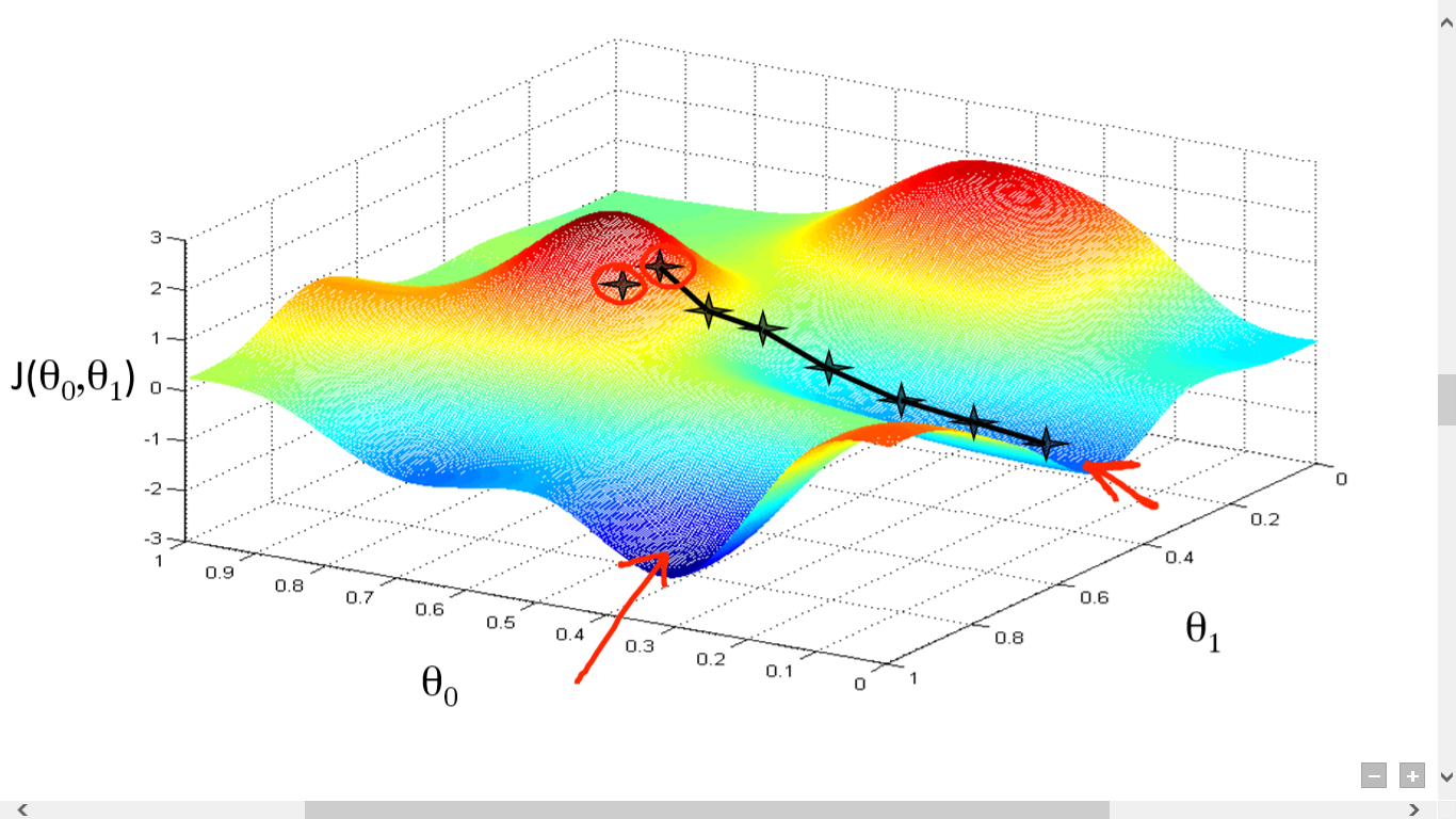
The direction of the step is defined by derivative of the cost function in current point.
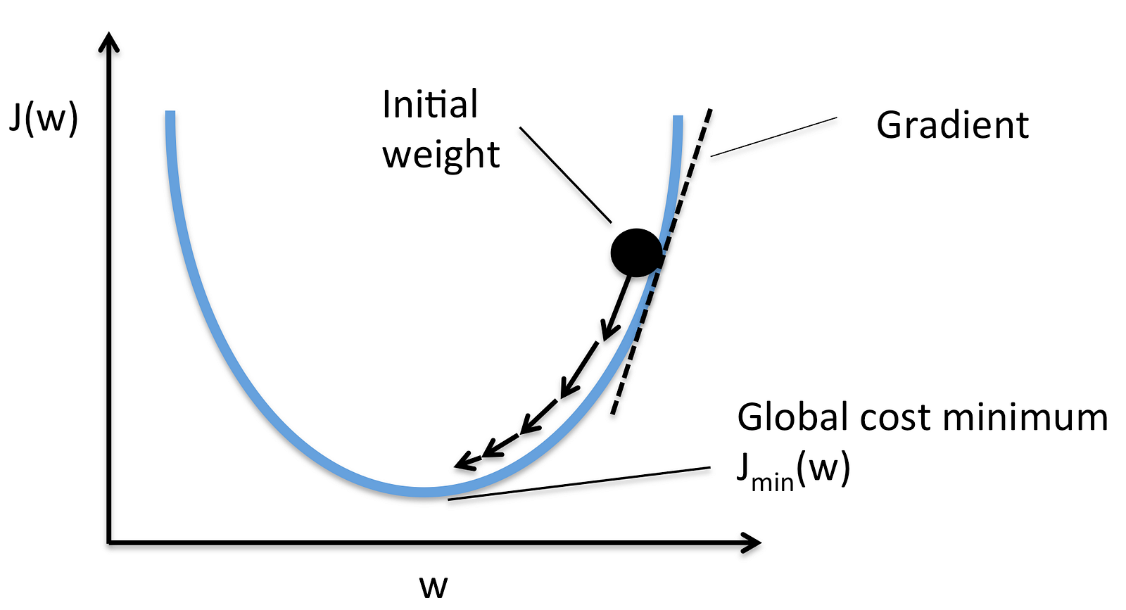
Once we decided what direction we need to go we need to decide what the size of the step we need to take.
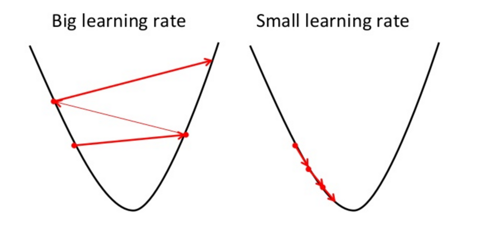
We need to simultaneously update  for _j = 0, 1, ..., n_


 - the learning rate, the constant that defines the size of the gradient descent step
 - _j<sup>th</sup>_ feature value of the _i<sup>th</sup>_ training example
 - input (features) of _i<sup>th</sup>_ training example
_y<sup>i</sup>_ - output of _i<sup>th</sup>_ training example
_m_ - number of training examples
_n_ - number of features
> When we use term "batch" for gradient descent it means that each step of gradient descent uses **all** the training examples (as you might see from the formula above).
## Feature Scaling
To make linear regression and gradient descent algorithm work correctly we need to make sure that features are on a similar scale.

For example "apartment size" feature (e.g. 120 m<sup>2</sup>) is much bigger than the "number of rooms" feature (e.g. 2).
In order to scale the features we need to do **mean normalization**

 - _j<sup>th</sup>_ feature value of the _i<sup>th</sup>_ training example
 - average value of _j<sup>th</sup>_ feature in training set
 - the range (_max - min_) of _j<sup>th</sup>_ feature in training set.
## Polynomial Regression
Polynomial regression is a form of regression analysis in which the relationship between the independent variable _x_ and the dependent variable _y_ is modelled as an _n<sup>th</sup>_ degree polynomial in _x_.
Although polynomial regression fits a nonlinear model to the data, as a statistical estimation problem it is linear, in the sense that the hypothesis function is linear in the unknown parameters that are estimated from the data. For this reason, polynomial regression is considered to be a special case of multiple linear regression.

Example of a cubic polynomial regression, which is a type of linear regression.
You may form polynomial regression by adding new polynomial features.
For example if the price of the apartment is in non-linear dependency of its size then you might add several new size-related features.

## Normal Equation
There is a closed-form solution to linear regression exists and it looks like the following:

Using this formula does not require any feature scaling, and you will get an exact solution in one calculation: there is no “loop until convergence” like in gradient descent.
## Regularization
### Overfitting Problem
If we have too many features, the learned hypothesis may fit the **training** set very well:

**But** it may fail to generalize to **new** examples (let's say predict prices on new example of detecting if new messages are spam).
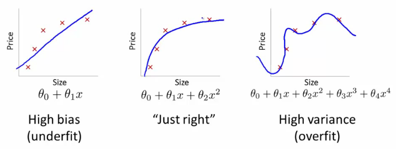
### Solution to Overfitting
Here are couple of options that may be addressed:
- Reduce the number of features
- Manually select which features to keep
- Model selection algorithm
- Regularization
- Keep all the features, but reduce magnitude/values of model parameters (thetas).
- Works well when we have a lot of features, each of which contributes a bit to predicting _y_.
Regularization works by adding regularization parameter to the **cost function**:

> Note that you should not regularize the parameter .
 - regularization parameter
In this case the **gradient descent** formula will look like the following:

## References
- [Machine Learning on Coursera](https://www.coursera.org/learn/machine-learning)
- [Linear Regression on Wikipedia](https://en.wikipedia.org/wiki/Linear_regression)
- [Gradient Descent on Wikipedia](https://en.wikipedia.org/wiki/Gradient_descent)
- [Gradient Descent by Suryansh S.](https://hackernoon.com/gradient-descent-aynk-7cbe95a778da)
- [Gradient Descent by Niklas Donges](https://towardsdatascience.com/gradient-descent-in-a-nutshell-eaf8c18212f0)
- [Overfitting on GeeksForGeeks](https://www.geeksforgeeks.org/underfitting-and-overfitting-in-machine-learning/)
================================================
FILE: homemade/linear_regression/__init__.py
================================================
"""Linear Regression Module"""
from .linear_regression import LinearRegression
================================================
FILE: homemade/linear_regression/linear_regression.py
================================================
"""Linear Regression Module"""
# Import dependencies.
import numpy as np
from ..utils.features import prepare_for_training
class LinearRegression:
# pylint: disable=too-many-instance-attributes
"""Linear Regression Class"""
def __init__(self, data, labels, polynomial_degree=0, sinusoid_degree=0, normalize_data=True):
# pylint: disable=too-many-arguments
"""Linear regression constructor.
:param data: training set.
:param labels: training set outputs (correct values).
:param polynomial_degree: degree of additional polynomial features.
:param sinusoid_degree: multipliers for sinusoidal features.
:param normalize_data: flag that indicates that features should be normalized.
"""
# Normalize features and add ones column.
(
data_processed,
features_mean,
features_deviation
) = prepare_for_training(data, polynomial_degree, sinusoid_degree, normalize_data)
self.data = data_processed
self.labels = labels
self.features_mean = features_mean
self.features_deviation = features_deviation
self.polynomial_degree = polynomial_degree
self.sinusoid_degree = sinusoid_degree
self.normalize_data = normalize_data
# Initialize model parameters.
num_features = self.data.shape[1]
self.theta = np.zeros((num_features, 1))
def train(self, alpha, lambda_param=0, num_iterations=500):
"""Trains linear regression.
:param alpha: learning rate (the size of the step for gradient descent)
:param lambda_param: regularization parameter
:param num_iterations: number of gradient descent iterations.
"""
# Run gradient descent.
cost_history = self.gradient_descent(alpha, lambda_param, num_iterations)
return self.theta, cost_history
def gradient_descent(self, alpha, lambda_param, num_iterations):
"""Gradient descent.
It calculates what steps (deltas) should be taken for each theta parameter in
order to minimize the cost function.
:param alpha: learning rate (the size of the step for gradient descent)
:param lambda_param: regularization parameter
:param num_iterations: number of gradient descent iterations.
"""
# Initialize J_history with zeros.
cost_history = []
for _ in range(num_iterations):
# Perform a single gradient step on the parameter vector theta.
self.gradient_step(alpha, lambda_param)
# Save the cost J in every iteration.
cost_history.append(self.cost_function(self.data, self.labels, lambda_param))
return cost_history
def gradient_step(self, alpha, lambda_param):
"""Gradient step.
Function performs one step of gradient descent for theta parameters.
:param alpha: learning rate (the size of the step for gradient descent)
:param lambda_param: regularization parameter
"""
# Calculate the number of training examples.
num_examples = self.data.shape[0]
# Predictions of hypothesis on all m examples.
predictions = LinearRegression.hypothesis(self.data, self.theta)
# The difference between predictions and actual values for all m examples.
delta = predictions - self.labels
# Calculate regularization parameter.
reg_param = 1 - alpha * lambda_param / num_examples
# Create theta shortcut.
theta = self.theta
# Vectorized version of gradient descent.
theta = theta * reg_param - alpha * (1 / num_examples) * (delta.T @ self.data).T
# We should NOT regularize the parameter theta_zero.
theta[0] = theta[0] - alpha * (1 / num_examples) * (self.data[:, 0].T @ delta).T
self.theta = theta
def get_cost(self, data, labels, lambda_param):
"""Get the cost value for specific data set.
:param data: the set of training or test data.
:param labels: training set outputs (correct values).
:param lambda_param: regularization parameter
"""
data_processed = prepare_for_training(
data,
self.polynomial_degree,
self.sinusoid_degree,
self.normalize_data,
)[0]
return self.cost_function(data_processed, labels, lambda_param)
def cost_function(self, data, labels, lambda_param):
"""Cost function.
It shows how accurate our model is based on current model parameters.
:param data: the set of training or test data.
:param labels: training set outputs (correct values).
:param lambda_param: regularization parameter
"""
# Calculate the number of training examples and features.
num_examples = data.shape[0]
# Get the difference between predictions and correct output values.
delta = LinearRegression.hypothesis(data, self.theta) - labels
# Calculate regularization parameter.
# Remember that we should not regularize the parameter theta_zero.
theta_cut = self.theta[1:, 0]
reg_param = lambda_param * (theta_cut.T @ theta_cut)
# Calculate current predictions cost.
cost = (1 / 2 * num_examples) * (delta.T @ delta + reg_param)
# Let's extract cost value from the one and only cost numpy matrix cell.
return cost[0][0]
def predict(self, data):
"""Predict the output for data_set input based on trained theta values
:param data: training set of features.
"""
# Normalize features and add ones column.
data_processed = prepare_for_training(
data,
self.polynomial_degree,
self.sinusoid_degree,
self.normalize_data,
)[0]
# Do predictions using model hypothesis.
predictions = LinearRegression.hypothesis(data_processed, self.theta)
return predictions
@staticmethod
def hypothesis(data, theta):
"""Hypothesis function.
It predicts the output values y based on the input values X and model parameters.
:param data: data set for what the predictions will be calculated.
:param theta: model params.
:return: predictions made by model based on provided theta.
"""
predictions = data @ theta
return predictions
================================================
FILE: homemade/logistic_regression/README.md
================================================
# Logistic Regression
## Jupyter Demos
▶️ [Demo | Logistic Regression With Linear Boundary](https://nbviewer.jupyter.org/github/trekhleb/homemade-machine-learning/blob/master/notebooks/logistic_regression/logistic_regression_with_linear_boundary_demo.ipynb) - predict Iris flower `class` based on `petal_length` and `petal_width`
▶️ [Demo | Logistic Regression With Non-Linear Boundary](https://nbviewer.jupyter.org/github/trekhleb/homemade-machine-learning/blob/master/notebooks/logistic_regression/logistic_regression_with_non_linear_boundary_demo.ipynb) - predict microchip `validity` based on `param_1` and `param_2`
▶️ [Demo | Multivariate Logistic Regression | MNIST](https://nbviewer.jupyter.org/github/trekhleb/homemade-machine-learning/blob/master/notebooks/logistic_regression/multivariate_logistic_regression_demo.ipynb) - recognize handwritten digits from `28x28` pixel images.
▶️ [Demo | Multivariate Logistic Regression | Fashion MNIST](https://nbviewer.jupyter.org/github/trekhleb/homemade-machine-learning/blob/master/notebooks/logistic_regression/multivariate_logistic_regression_fashion_demo.ipynb) - recognize clothes types from `28x28` pixel images.
## Definition
**Logistic regression** is the appropriate regression analysis to conduct when the dependent variable is dichotomous (binary). Like all regression analyses, the logistic regression is a predictive analysis. Logistic regression is used to describe data and to explain the relationship between one dependent binary variable and one or more nominal, ordinal, interval or ratio-level independent variables.
Logistic Regression is used when the dependent variable (target) is categorical.
For example:
- To predict whether an email is spam (1) or (0).
- Whether online transaction is fraudulent (1) or not (0).
- Whether the tumor is malignant (1) or not (0).
In other words the dependant variable (output) for logistic regression model may be described as:

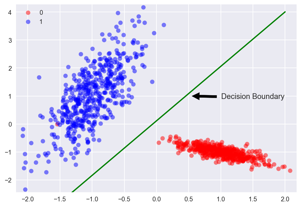
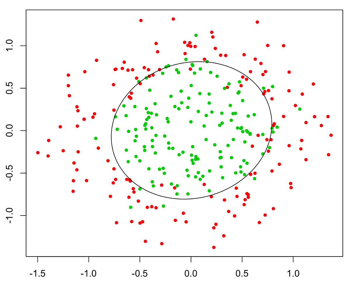
## Training Set
Training set is an input data where for every predefined set of features _x_ we have a correct classification _y_.

_m_ - number of training set examples.

For convenience of notation, define:


## Hypothesis (the Model)
The equation that gets features and parameters as an input and predicts the value as an output (i.e. predict if the email is spam or not based on some email characteristics).

Where _g()_ is a **sigmoid function**.


Now we my write down the hypothesis as follows:


## Cost Function
Function that shows how accurate the predictions of the hypothesis are with current set of parameters.


Cost function may be simplified to the following one-liner:

## Batch Gradient Descent
Gradient descent is an iterative optimization algorithm for finding the minimum of a cost function described above. To find a local minimum of a function using gradient descent, one takes steps proportional to the negative of the gradient (or approximate gradient) of the function at the current point.
Picture below illustrates the steps we take going down of the hill to find local minimum.

The direction of the step is defined by derivative of the cost function in current point.

Once we decided what direction we need to go we need to decide what the size of the step we need to take.

We need to simultaneously update  for _j = 0, 1, ..., n_


 - the learning rate, the constant that defines the size of the gradient descent step
 - _j<sup>th</sup>_ feature value of the _i<sup>th</sup>_ training example
 - input (features) of _i<sup>th</sup>_ training example
_y<sup>i</sup>_ - output of _i<sup>th</sup>_ training example
_m_ - number of training examples
_n_ - number of features
> When we use term "batch" for gradient descent it means that each step of gradient descent uses **all** the training examples (as you might see from the formula above).
## Multi-class Classification (One-vs-All)
Very often we need to do not just binary (0/1) classification but rather multi-class ones, like:
- Weather: Sunny, Cloudy, Rain, Snow
- Email tagging: Work, Friends, Family
To handle these type of issues we may train a logistic regression classifier  several times for each class _i_ to predict the probability that _y = i_.

## Regularization
### Overfitting Problem
If we have too many features, the learned hypothesis may fit the **training** set very well:

**But** it may fail to generalize to **new** examples (let's say predict prices on new example of detecting if new messages are spam).
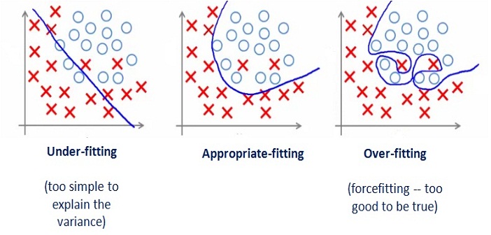
### Solution to Overfitting
Here are couple of options that may be addressed:
- Reduce the number of features
- Manually select which features to keep
- Model selection algorithm
- Regularization
- Keep all the features, but reduce magnitude/values of model parameters (thetas).
- Works well when we have a lot of features, each of which contributes a bit to predicting _y_.
Regularization works by adding regularization parameter to the **cost function**:

 - regularization parameter
> Note that you should not regularize the parameter .
In this case the **gradient descent** formula will look like the following:

## References
- [Machine Learning on Coursera](https://www.coursera.org/learn/machine-learning)
- [Sigmoid Function on Wikipedia](https://en.wikipedia.org/wiki/Sigmoid_function)
- [Gradient Descent on Wikipedia](https://en.wikipedia.org/wiki/Gradient_descent)
- [Gradient Descent by Suryansh S.](https://hackernoon.com/gradient-descent-aynk-7cbe95a778da)
- [Gradient Descent by Niklas Donges](https://towardsdatascience.com/gradient-descent-in-a-nutshell-eaf8c18212f0)
- [One vs All on Stackexchange](https://stats.stackexchange.com/questions/318520/many-binary-classifiers-vs-single-multiclass-classifier)
- [Logistic Regression by Rohan Kapur](https://ayearofai.com/rohan-1-when-would-i-even-use-a-quadratic-equation-in-the-real-world-13f379edab3b)
- [Overfitting on GeeksForGeeks](https://www.geeksforgeeks.org/underfitting-and-overfitting-in-machine-learning/)
================================================
FILE: homemade/logistic_regression/__init__.py
================================================
"""Logistic Regression Module"""
from .logistic_regression import LogisticRegression
================================================
FILE: homemade/logistic_regression/logistic_regression.py
================================================
"""Logistic Regression Module"""
import numpy as np
from scipy.optimize import minimize
from ..utils.features import prepare_for_training
from ..utils.hypothesis import sigmoid
class LogisticRegression:
# pylint: disable=too-many-instance-attributes
"""Logistic Regression Class"""
def __init__(self, data, labels, polynomial_degree=0, sinusoid_degree=0, normalize_data=False):
# pylint: disable=too-many-arguments
"""Logistic regression constructor.
:param data: training set.
:param labels: training set outputs (correct values).
:param polynomial_degree: degree of additional polynomial features.
:param sinusoid_degree: multipliers for sinusoidal features.
:param normalize_data: flag that indicates that features should be normalized.
"""
# Normalize features and add ones column.
(
data_processed,
mean,
deviation
) = prepare_for_training(data, polynomial_degree, sinusoid_degree, normalize_data)
self.data = data_processed
self.labels = labels
self.unique_labels = np.unique(labels)
self.features_mean = mean
self.features_deviation = deviation
self.polynomial_degree = polynomial_degree
self.sinusoid_degree = sinusoid_degree
self.normalize_data = normalize_data
# Initialize model parameters.
num_features = self.data.shape[1]
num_unique_labels = np.unique(labels).shape[0]
self.thetas = np.zeros((num_unique_labels, num_features))
def train(self, lambda_param=0, max_iterations=1000):
"""Trains logistic regression.
:param lambda_param: regularization parameter
:param max_iterations: maximum number of gradient descent iterations.
"""
# Init cost history array.
cost_histories = []
# Use One-vs-All approach and train the model several times for each label class.
num_features = self.data.shape[1]
# Train the model to distinguish each label particularly.
for label_index, unique_label in enumerate(self.unique_labels):
current_initial_theta = np.copy(self.thetas[label_index]).reshape((num_features, 1))
# Convert labels to array of 0s and 1s for current label class.
current_labels = (self.labels == unique_label).astype(float)
# Run gradient descent.
(current_theta, cost_history) = LogisticRegression.gradient_descent(
self.data,
current_labels,
current_initial_theta,
lambda_param,
max_iterations,
)
self.thetas[label_index] = current_theta.T
cost_histories.append(cost_history)
# return self.theta, cost_history
return self.thetas, cost_histories
def predict(self, data):
"""Prediction function"""
num_examples = data.shape[0]
data_processed = prepare_for_training(
data,
self.polynomial_degree,
self.sinusoid_degree,
self.normalize_data
)[0]
probability_predictions = LogisticRegression.hypothesis(data_processed, self.thetas.T)
max_probability_indices = np.argmax(probability_predictions, axis=1)
class_predictions = np.empty(max_probability_indices.shape, dtype=object)
for index, label in enumerate(self.unique_labels):
class_predictions[max_probability_indices == index] = label
return class_predictions.reshape((num_examples, 1))
@staticmethod
def gradient_descent(data, labels, initial_theta, lambda_param, max_iteration):
"""Gradient descent function.
Iteratively optimizes theta model parameters.
:param data: the set of training or test data.
:param labels: training set outputs (0 or 1 that defines the class of an example).
:param initial_theta: initial model parameters.
:param lambda_param: regularization parameter.
:param max_iteration: maximum number of gradient descent steps.
"""
# Initialize cost history list.
cost_history = []
# Calculate the number of features.
num_features = data.shape[1]
# Launch gradient descent.
minification_result = minimize(
# Function that we're going to minimize.
lambda current_theta: LogisticRegression.cost_function(
data, labels, current_theta.reshape((num_features, 1)), lambda_param
),
# Initial values of model parameter.
initial_theta,
# We will use conjugate gradient algorithm.
method='CG',
# Function that will help to calculate gradient direction on each step.
jac=lambda current_theta: LogisticRegression.gradient_step(
data, labels, current_theta.reshape((num_features, 1)), lambda_param
),
# Record gradient descent progress for debugging.
callback=lambda current_theta: cost_history.append(LogisticRegression.cost_function(
data, labels, current_theta.reshape((num_features, 1)), lambda_param
)),
options={'maxiter': max_iteration}
)
# Throw an error in case if gradient descent ended up with error.
if not minification_result.success:
raise ArithmeticError('Can not minimize cost function: ' + minification_result.message)
# Reshape the final version of model parameters.
optimized_theta = minification_result.x.reshape((num_features, 1))
return optimized_theta, cost_history
@staticmethod
def gradient_step(data, labels, theta, lambda_param):
"""GRADIENT STEP function.
It performs one step of gradient descent for theta parameters.
:param data: the set of training or test data.
:param labels: training set outputs (0 or 1 that defines the class of an example).
:param theta: model parameters.
:param lambda_param: regularization parameter.
"""
# Initialize number of training examples.
num_examples = labels.shape[0]
# Calculate hypothesis predictions and difference with labels.
predictions = LogisticRegression.hypothesis(data, theta)
label_diff = predictions - labels
# Calculate regularization parameter.
regularization_param = (lambda_param / num_examples) * theta
# Calculate gradient steps.
gradients = (1 / num_examples) * (data.T @ label_diff)
regularized_gradients = gradients + regularization_param
# We should NOT regularize the parameter theta_zero.
regularized_gradients[0] = (1 / num_examples) * (data[:, [0]].T @ label_diff)
return regularized_gradients.T.flatten()
@staticmethod
def cost_function(data, labels, theta, lambda_param):
"""Cost function.
It shows how accurate our model is based on current model parameters.
:param data: the set of training or test data.
:param labels: training set outputs (0 or 1 that defines the class of an example).
:param theta: model parameters.
:param lambda_param: regularization parameter.
"""
# Calculate the number of training examples and features.
num_examples = data.shape[0]
# Calculate hypothesis.
predictions = LogisticRegression.hypothesis(data, theta)
# Calculate regularization parameter
# Remember that we should not regularize the parameter theta_zero.
theta_cut = theta[1:, [0]]
reg_param = (lambda_param / (2 * num_examples)) * (theta_cut.T @ theta_cut)
# Calculate current predictions cost.
y_is_set_cost = labels[labels == 1].T @ np.log(predictions[labels == 1])
y_is_not_set_cost = (1 - labels[labels == 0]).T @ np.log(1 - predictions[labels == 0])
cost = (-1 / num_examples) * (y_is_set_cost + y_is_not_set_cost) + reg_param
# Let's extract cost value from the one and only cost numpy matrix cell.
return cost[0][0]
@staticmethod
def hypothesis(data, theta):
"""Hypothesis function.
It predicts the output values y based on the input values X and model parameters.
:param data: data set for what the predictions will be calculated.
:param theta: model params.
:return: predictions made by model based on provided theta.
"""
predictions = sigmoid(data @ theta)
return predictions
================================================
FILE: homemade/neural_network/README.md
================================================
# Neural Network
## Jupyter Demos
▶️ [Demo | Multilayer Perceptron | MNIST](https://nbviewer.jupyter.org/github/trekhleb/homemade-machine-learning/blob/master/notebooks/neural_network/multilayer_perceptron_demo.ipynb) - recognize handwritten digits from `28x28` pixel images.
▶️ [Demo | Multilayer Perceptron | Fashion MNIST](https://nbviewer.jupyter.org/github/trekhleb/homemade-machine-learning/blob/master/notebooks/neural_network/multilayer_perceptron_fashion_demo.ipynb) - recognize the type of clothes (Dress, Coat, Sandal, etc.) from `28x28` pixel images.
## Definition
**Artificial neural networks** (ANN) or connectionist systems are computing systems vaguely inspired by the biological neural networks that constitute animal brains. The neural network itself isn't an algorithm, but rather a framework for many different machine learning algorithms to work together and process complex data inputs. Such systems "learn" to perform tasks by considering examples, generally without being programmed with any task-specific rules.
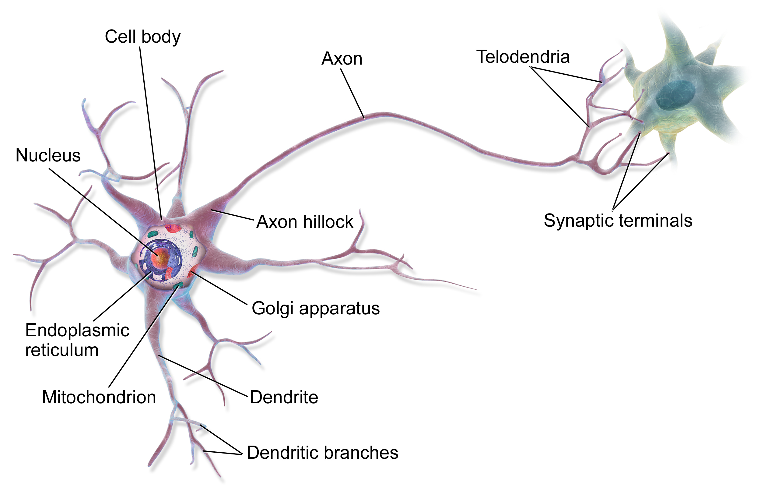
For example, in **image recognition**, they might learn to identify images that contain cats by analyzing example images that have been manually labeled as "cat" or "no cat" and using the results to identify cats in other images. They do this without any prior knowledge about cats, e.g., that they have fur, tails, whiskers and cat-like faces. Instead, they automatically generate identifying characteristics from the learning material that they process.
An ANN is based on a collection of connected units or nodes called **artificial neurons**, which loosely model the neurons in a biological brain. Each connection, like the synapses in a biological brain, can transmit a signal from one artificial neuron to another. An artificial neuron that receives a signal can process it and then signal additional artificial neurons connected to it.

In common ANN implementations, the signal at a connection between artificial neurons is a real number, and the output of each artificial neuron is computed by some non-linear function of the sum of its inputs. The connections between artificial neurons are called **edges**. Artificial neurons and edges typically have a **weight** that adjusts as learning proceeds. The weight increases or decreases the strength of the signal at a connection. Artificial neurons may have a threshold such that the signal is only sent if the aggregate signal crosses that threshold. Typically, artificial neurons are aggregated into layers. Different layers may perform different kinds of transformations on their inputs. Signals travel from the first layer (the **input layer**), to the last layer (the **output layer**), possibly after traversing the **inner layers** multiple times.

A **multilayer perceptron (MLP)** is a class of feedforward artificial neural network. An MLP consists of, at least, three layers of nodes: an input layer, a hidden layer and an output layer. Except for the input nodes, each node is a neuron that uses a nonlinear activation function. MLP utilizes a supervised learning technique called backpropagation for training. Its multiple layers and non-linear activation distinguish MLP from a linear perceptron. It can distinguish data that is not linearly separable.
## Neuron Model (Logistic Unit)
Here is a model of one neuron unit.


Weights:

## Network Model (Set of Neurons)
Neural network consists of the neuron units described in the section above.
Let's take a look at simple example model with one hidden layer.

 - "activation" of unit _i_ in layer _j_.
 - matrix of weights controlling function mapping from layer _j_ to layer _j + 1_. For example for the first layer: .
 - total number of layers in network (3 in our example).
 - number of units (not counting bias unit) in layer _l_.
 - number of output units (1 in our example but could be any real number for multi-class classification).
## Multi-class Classification
In order to make neural network to work with multi-class notification we may use **One-vs-All** approach.
Let's say we want our network to distinguish if there is a _pedestrian_ or _car_ of _motorcycle_ or _truck_ is on the image.
In this case the output layer of our network will have 4 units (input layer will be much bigger and it will have all the pixel from the image. Let's say if all our images will be 20x20 pixels then the input layer will have 400 units each of which will contain the black-white color of the corresponding picture).


In this case we would expect our final hypothesis to have following values:


In this case for the training set:

We would have:

## Forward (or Feedforward) Propagation
Forward propagation is an interactive process of calculating activations for each layer starting from the input layer and going to the output layer.
For the simple network mentioned in a previous section above we're able to calculate activations for second layer based on the input layer and our network parameters:


The output layer activation will be calculated based on the hidden layer activations:

Where _g()_ function may be a sigmoid:


### Vectorized Implementation of Forward Propagation
Now let's convert previous calculations into more concise vectorized form.

To simplify previous activation equations let's introduce a _z_ variable:


> Don't forget to add bias units (activations) before propagating to the next layer.
> 


### Forward Propagation Example
Let's take the following network architecture with 4 layers (input layer, 2 hidden layers and output layer) as an example:

In this case the forward propagation steps would look like the following:

## Cost Function
The cost function for the neuron network is quite similar to the logistic regression cost function.


## Backpropagation
### Gradient Computation
Backpropagation algorithm has the same purpose as gradient descent for linear or logistic regression - it corrects the values of thetas to minimize a cost function.
In other words we need to be able to calculate partial derivative of cost function for each theta.


Let's assume that:
 - "error" of node _j_ in layer _l_.
For each output unit (layer _L = 4_):

Or in vectorized form:


 - sigmoid gradient.

Now we may calculate the gradient step:

### Backpropagation Algorithm
For training set

We need to set:


## Random Initialization
Before starting forward propagation we need to initialize Theta parameters. We can not assign zero to all thetas since this would make our network useless because every neuron of the layer will learn the same as its siblings. In other word we need to **break the symmetry**. In order to do so we need to initialize thetas to some small random initial values:

## References
- [Machine Learning on Coursera](https://www.coursera.org/learn/machine-learning)
- [But what is a Neural Network? By 3Blue1Brown](https://www.youtube.com/watch?v=aircAruvnKk)
- [Neural Network on Wikipedia](https://en.wikipedia.org/wiki/Artificial_neural_network)
- [TensorFlow Neural Network Playground](https://playground.tensorflow.org/)
- [Deep Learning by Carnegie Mellon University](https://insights.sei.cmu.edu/sei_blog/2018/02/deep-learning-going-deeper-toward-meaningful-patterns-in-complex-data.html)
================================================
FILE: homemade/neural_network/__init__.py
================================================
"""Neural Network Module"""
from .multilayer_perceptron import MultilayerPerceptron
================================================
FILE: homemade/neural_network/multilayer_perceptron.py
================================================
"""Neural Network Module"""
import numpy as np
from ..utils.features import prepare_for_training
from ..utils.hypothesis import sigmoid, sigmoid_gradient
class MultilayerPerceptron:
"""Multilayer Perceptron Class"""
# pylint: disable=too-many-arguments
def __init__(self, data, labels, layers, epsilon, normalize_data=False):
"""Multilayer perceptron constructor.
:param data: training set.
:param labels: training set outputs (correct values).
:param layers: network layers configuration.
:param epsilon: Defines the range for initial theta values.
:param normalize_data: flag that indicates that features should be normalized.
"""
# Normalize features and add ones column.
data_processed = prepare_for_training(data, normalize_data=normalize_data)[0]
self.data = data_processed
self.labels = labels
self.layers = layers
self.epsilon = epsilon
self.normalize_data = normalize_data
# Randomly initialize the weights for each neural network layer.
self.thetas = MultilayerPerceptron.thetas_init(layers, epsilon)
def train(self, regularization_param=0, max_iterations=1000, alpha=1):
"""Train the model"""
# Flatten model thetas for gradient descent.
unrolled_thetas = MultilayerPerceptron.thetas_unroll(self.thetas)
# Run gradient descent.
(optimized_thetas, cost_history) = MultilayerPerceptron.gradient_descent(
self.data,
self.labels,
unrolled_thetas,
self.layers,
regularization_param,
max_iterations,
alpha
)
# Memorize optimized theta parameters.
self.thetas = MultilayerPerceptron.thetas_roll(optimized_thetas, self.layers)
return self.thetas, cost_history
def predict(self, data):
"""Predictions function that does classification using trained model"""
data_processed = prepare_for_training(data, normalize_data=self.normalize_data)[0]
num_examples = data_processed.shape[0]
# Do feedforward propagation with trained neural network params.
predictions = MultilayerPerceptron.feedforward_propagation(
data_processed, self.thetas, self.layers
)
# Return the index of the output neuron with the highest probability.
return np.argmax(predictions, axis=1).reshape((num_examples, 1))
@staticmethod
def gradient_descent(
data, labels, unrolled_theta, layers, regularization_param, max_iteration, alpha
):
# pylint: disable=too-many-arguments
"""Gradient descent function.
Iteratively optimizes theta model parameters.
:param data: the set of training or test data.
:param labels: training set outputs (0 or 1 that defines the class of an example).
:param unrolled_theta: initial model parameters.
:param layers: model layers configuration.
:param regularization_param: regularization parameter.
:param max_iteration: maximum number of gradient descent steps.
:param alpha: gradient descent step size.
"""
optimized_theta = unrolled_theta
# Initialize cost history list.
cost_history = []
for _ in range(max_iteration):
# Get current cost.
cost = MultilayerPerceptron.cost_function(
data,
labels,
MultilayerPerceptron.thetas_roll(optimized_theta, layers),
layers,
regularization_param
)
# Save current cost value to build plots later.
cost_history.append(cost)
# Get the next gradient step directions.
theta_gradient = MultilayerPerceptron.gradient_step(
data, labels, optimized_theta, layers, regularization_param
)
# Adjust theta values according to the next gradient step.
optimized_theta = optimized_theta - alpha * theta_gradient
return optimized_theta, cost_history
@staticmethod
def gradient_step(data, labels, unrolled_thetas, layers, regularization_param):
"""Gradient step function.
Computes the cost and gradient of the neural network for unrolled theta parameters.
:param data: training set.
:param labels: training set labels.
:param unrolled_thetas: model parameters.
:param layers: model layers configuration.
:param regularization_param: parameters that fights with model over-fitting.
"""
# Reshape nn_params back into the matrix parameters.
thetas = MultilayerPerceptron.thetas_roll(unrolled_thetas, layers)
# Do backpropagation.
thetas_rolled_gradients = MultilayerPerceptron.back_propagation(
data, labels, thetas, layers, regularization_param
)
# Unroll thetas gradients.
thetas_unrolled_gradients = MultilayerPerceptron.thetas_unroll(thetas_rolled_gradients)
return thetas_unrolled_gradients
# pylint: disable=R0914
@staticmethod
def cost_function(data, labels, thetas, layers, regularization_param):
"""Cost function.
It shows how accurate our model is based on current model parameters.
:param data: the set of training or test data.
:param labels: training set outputs (0 or 1 that defines the class of an example).
:param thetas: model parameters.
:param layers: layers configuration.
:param regularization_param: regularization parameter.
"""
# Get total number of layers.
num_layers = len(layers)
# Get total number of training examples.
num_examples = data.shape[0]
# Get the size of output layer (number of labels).
num_labels = layers[-1]
# Feedforward the neural network.
predictions = MultilayerPerceptron.feedforward_propagation(data, thetas, layers)
# Compute the cost.
# For now the labels vector is just an expected number for each input example.
# We need to convert every result from number to vector that will illustrate
# the output we're expecting. For example instead of having just number 5
# we want to expect [0 0 0 0 1 0 0 0 0 0]. The bit is set for 5th position.
bitwise_labels = np.zeros((num_examples, num_labels))
for example_index in range(num_examples):
bitwise_labels[example_index][labels[example_index][0]] = 1
# Calculate regularization parameter.
theta_square_sum = 0
for layer_index in range(num_layers - 1):
theta = thetas[layer_index]
# Don't try to regularize bias thetas.
theta_square_sum = theta_square_sum + np.sum(theta[:, 1:] ** 2)
regularization = (regularization_param / (2 * num_examples)) * theta_square_sum
# Calculate the cost with regularization.
bit_set_cost = np.sum(np.log(predictions[bitwise_labels == 1]))
bit_not_set_cost = np.sum(np.log(1 - predictions[bitwise_labels == 0]))
cost = (-1 / num_examples) * (bit_set_cost + bit_not_set_cost) + regularization
return cost
@staticmethod
def feedforward_propagation(data, thetas, layers):
"""Feedforward propagation function"""
# Calculate the total number of layers.
num_layers = len(layers)
# Calculate the number of training examples.
num_examples = data.shape[0]
# Input layer (l=1)
in_layer_activation = data
# Propagate to hidden layers.
for layer_index in range(num_layers - 1):
theta = thetas[layer_index]
out_layer_activation = sigmoid(in_layer_activation @ theta.T)
# Add bias units.
out_layer_activation = np.hstack((np.ones((num_examples, 1)), out_layer_activation))
in_layer_activation = out_layer_activation
# Output layer should not contain bias units.
return in_layer_activation[:, 1:]
# pylint: disable=R0914
@staticmethod
def back_propagation(data, labels, thetas, layers, regularization_param):
"""Backpropagation function"""
# Get total number of layers.
num_layers = len(layers)
# Get total number of training examples and features.
(num_examples, num_features) = data.shape
# Get the number of possible output labels.
num_label_types = layers[-1]
# Initialize big delta - aggregated delta values for all training examples that will
# indicate how exact theta need to be changed.
deltas = {}
for layer_index in range(num_layers - 1):
in_count = layers[layer_index]
out_count = layers[layer_index + 1]
deltas[layer_index] = np.zeros((out_count, in_count + 1))
# Let's go through all examples.
for example_index in range(num_examples):
# We will store layers inputs and activations in order to re-use it later.
layers_inputs = {}
layers_activations = {}
# Setup input layer activations.
layer_activation = data[example_index, :].reshape((num_features, 1))
layers_activations[0] = layer_activation
# Perform a feedforward pass for current training example.
for layer_index in range(num_layers - 1):
layer_theta = thetas[layer_index]
layer_input = layer_theta @ layer_activation
layer_activation = np.vstack((np.array([[1]]), sigmoid(layer_input)))
layers_inputs[layer_index + 1] = layer_input
layers_activations[layer_index + 1] = layer_activation
# Remove bias units from the output activations.
output_layer_activation = layer_activation[1:, :]
# Calculate deltas.
# For input layer we don't calculate delta because we do not
# associate error with the input.
delta = {}
# Convert the output from number to vector (i.e. 5 to [0; 0; 0; 0; 1; 0; 0; 0; 0; 0])
bitwise_label = np.zeros((num_label_types, 1))
bitwise_label[labels[example_index][0]] = 1
# Calculate deltas for the output layer for current training example.
delta[num_layers - 1] = output_layer_activation - bitwise_label
# Calculate small deltas for hidden layers for current training example.
# The loops should go for the layers L, L-1, ..., 1.
for layer_index in range(num_layers - 2, 0, -1):
layer_theta = thetas[layer_index]
next_delta = delta[layer_index + 1]
layer_input = layers_inputs[layer_index]
# Add bias row to the layer input.
layer_input = np.vstack((np.array([[1]]), layer_input))
# Calculate row delta and take off the bias row from it.
delta[layer_index] = (layer_theta.T @ next_delta) * sigmoid_gradient(layer_input)
delta[layer_index] = delta[layer_index][1:, :]
# Accumulate the gradient (update big deltas).
for layer_index in range(num_layers - 1):
layer_delta = delta[layer_index + 1] @ layers_activations[layer_index].T
deltas[layer_index] = deltas[layer_index] + layer_delta
# Obtain un-regularized gradient for the neural network cost function.
for layer_index in range(num_layers - 1):
# Remember that we should NOT be regularizing the first column of theta.
current_delta = deltas[layer_index]
current_delta = np.hstack((np.zeros((current_delta.shape[0], 1)), current_delta[:, 1:]))
# Calculate regularization.
regularization = (regularization_param / num_examples) * current_delta
# Regularize deltas.
deltas[layer_index] = (1 / num_examples) * deltas[layer_index] + regularization
return deltas
@staticmethod
def thetas_init(layers, epsilon):
"""Randomly initialize the weights for each neural network layer
Each layer will have its own theta matrix W with L_in incoming connections and L_out
outgoing connections. Note that W will be set to a matrix of size(L_out, 1 + L_in) as the
first column of W handles the "bias" terms.
:param layers:
:param epsilon:
:return:
"""
# Get total number of layers.
num_layers = len(layers)
# Generate initial thetas for each layer.
thetas = {}
# Generate Thetas only for input and hidden layers.
# There is no need to generate Thetas for the output layer.
for layer_index in range(num_layers - 1):
in_count = layers[layer_index]
out_count = layers[layer_index + 1]
thetas[layer_index] = np.random.rand(out_count, in_count + 1) * 2 * epsilon - epsilon
return thetas
@staticmethod
def thetas_unroll(thetas):
"""Unrolls cells of theta matrices into one long vector."""
unrolled_thetas = np.array([])
num_theta_layers = len(thetas)
for theta_layer_index in range(num_theta_layers):
# Unroll cells into vector form.
unrolled_thetas = np.hstack((unrolled_thetas, thetas[theta_layer_index].flatten()))
return unrolled_thetas
@staticmethod
def thetas_roll(unrolled_thetas, layers):
"""Rolls NN params vector into the matrix"""
# Get total numbers of layers.
num_layers = len(layers)
# Init rolled thetas dictionary.
thetas = {}
unrolled_shift = 0
for layer_index in range(num_layers - 1):
in_count = layers[layer_index]
out_count = layers[layer_index + 1]
thetas_width = in_count + 1 # We need to remember about bias unit.
thetas_height = out_count
thetas_volume = thetas_width * thetas_height
# We need to remember about bias units when rolling up params.
start_index = unrolled_shift
end_index = unrolled_shift + thetas_volume
layer_thetas_unrolled = unrolled_thetas[start_index:end_index]
thetas[layer_index] = layer_thetas_unrolled.reshape((thetas_height, thetas_width))
# Shift frame to the right.
unrolled_shift = unrolled_shift + thetas_volume
return thetas
================================================
FILE: homemade/utils/__init__.py
================================================
================================================
FILE: homemade/utils/features/__init__.py
================================================
"""Dataset Features Related Utils"""
from .normalize import normalize
from .generate_polynomials import generate_polynomials
from .generate_sinusoids import generate_sinusoids
from .prepare_for_training import prepare_for_training
================================================
FILE: homemade/utils/features/generate_polynomials.py
================================================
"""Add polynomial features to the features set"""
import numpy as np
from .normalize import normalize
def generate_polynomials(dataset, polynomial_degree, normalize_data=False):
"""Extends data set with polynomial features of certain degree.
Returns a new feature array with more features, comprising of
x1, x2, x1^2, x2^2, x1*x2, x1*x2^2, etc.
:param dataset: dataset that we want to generate polynomials for.
:param polynomial_degree: the max power of new features.
:param normalize_data: flag that indicates whether polynomials need to normalized or not.
"""
# Split features on two halves.
features_split = np.array_split(dataset, 2, axis=1)
dataset_1 = features_split[0]
dataset_2 = features_split[1]
# Extract sets parameters.
(num_examples_1, num_features_1) = dataset_1.shape
(num_examples_2, num_features_2) = dataset_2.shape
# Check if two sets have equal amount of rows.
if num_examples_1 != num_examples_2:
raise ValueError('Can not generate polynomials for two sets with different number of rows')
# Check if at list one set has features.
if num_features_1 == 0 and num_features_2 == 0:
raise ValueError('Can not generate polynomials for two sets with no columns')
# Replace empty set with non-empty one.
if num_features_1 == 0:
dataset_1 = dataset_2
elif num_features_2 == 0:
dataset_2 = dataset_1
# Make sure that sets have the same number of features in order to be able to multiply them.
num_features = num_features_1 if num_features_1 < num_examples_2 else num_features_2
dataset_1 = dataset_1[:, :num_features]
dataset_2 = dataset_2[:, :num_features]
# Create polynomials matrix.
polynomials = np.empty((num_examples_1, 0))
# Generate polynomial features of specified degree.
for i in range(1, polynomial_degree + 1):
for j in range(i + 1):
polynomial_feature = (dataset_1 ** (i - j)) * (dataset_2 ** j)
polynomials = np.concatenate((polynomials, polynomial_feature), axis=1)
# Normalize polynomials if needed.
if normalize_data:
polynomials = normalize(polynomials)[0]
# Return generated polynomial features.
return polynomials
================================================
FILE: homemade/utils/features/generate_sinusoids.py
================================================
"""Add sinusoid features to the features set"""
import numpy as np
def generate_sinusoids(dataset, sinusoid_degree):
"""Extends data set with sinusoid features.
Returns a new feature array with more features, comprising of
sin(x).
:param dataset: data set.
:param sinusoid_degree: multiplier for sinusoid parameter multiplications
"""
# Create sinusoids matrix.
num_examples = dataset.shape[0]
sinusoids = np.empty((num_examples, 0))
# Generate sinusoid features of specified degree.
for degree in range(1, sinusoid_degree + 1):
sinusoid_features = np.sin(degree * dataset)
sinusoids = np.concatenate((sinusoids, sinusoid_features), axis=1)
# Return generated sinusoidal features.
return sinusoids
================================================
FILE: homemade/utils/features/normalize.py
================================================
"""Normalize features"""
import numpy as np
def normalize(features):
"""Normalize features.
Normalizes input features X. Returns a normalized version of X where the mean value of
each feature is 0 and deviation is close to 1.
:param features: set of features.
:return: normalized set of features.
"""
# Copy original array to prevent it from changes.
features_normalized = np.copy(features).astype(float)
# Get average values for each feature (column) in X.
features_mean = np.mean(features, 0)
# Calculate the standard deviation for each feature.
features_deviation = np.std(features, 0)
# Subtract mean values from each feature (column) of every example (row)
# to make all features be spread around zero.
if features.shape[0] > 1:
features_normalized -= features_mean
# Normalize each feature values so that all features are close to [-1:1] boundaries.
# Also prevent division by zero error.
features_deviation[features_deviation == 0] = 1
features_normalized /= features_deviation
return features_normalized, features_mean, features_deviation
================================================
FILE: homemade/utils/features/prepare_for_training.py
================================================
"""Prepares the dataset for training"""
import numpy as np
from .normalize import normalize
from .generate_sinusoids import generate_sinusoids
from .generate_polynomials import generate_polynomials
def prepare_for_training(data, polynomial_degree=0, sinusoid_degree=0, normalize_data=True):
"""Prepares data set for training on prediction"""
# Calculate the number of examples.
num_examples = data.shape[0]
# Prevent original data from being modified.
data_processed = np.copy(data)
# Normalize data set.
features_mean = 0
features_deviation = 0
data_normalized = data_processed
if normalize_data:
(
data_normalized,
features_mean,
features_deviation
) = normalize(data_processed)
# Replace processed data with normalized processed data.
# We need to have normalized data below while we will adding polynomials and sinusoids.
data_processed = data_normalized
# Add sinusoidal features to the dataset.
if sinusoid_degree > 0:
sinusoids = generate_sinusoids(data_normalized, sinusoid_degree)
data_processed = np.concatenate((data_processed, sinusoids), axis=1)
# Add polynomial features to data set.
if polynomial_degree > 0:
polynomials = generate_polynomials(data_normalized, polynomial_degree, normalize_data)
data_processed = np.concatenate((data_processed, polynomials), axis=1)
# Add a column of ones to X.
data_processed = np.hstack((np.ones((num_examples, 1)), data_processed))
return data_processed, features_mean, features_deviation
================================================
FILE: homemade/utils/hypothesis/__init__.py
================================================
"""Dataset Hypothesis Related Utils"""
from .sigmoid import sigmoid
from .sigmoid_gradient import sigmoid_gradient
================================================
FILE: homemade/utils/hypothesis/sigmoid.py
================================================
"""Sigmoid function"""
import numpy as np
def sigmoid(matrix):
"""Applies sigmoid function to NumPy matrix"""
return 1 / (1 + np.exp(-matrix))
================================================
FILE: homemade/utils/hypothesis/sigmoid_gradient.py
================================================
"""Sigmoid gradient function"""
from .sigmoid import sigmoid
def sigmoid_gradient(matrix):
"""Computes the gradient of the sigmoid function evaluated at z."""
return sigmoid(matrix) * (1 - sigmoid(matrix))
================================================
FILE: images/machine-learning-map.xml
================================================
<mxfile userAgent="Mozilla/5.0 (Macintosh; Intel Mac OS X 10_14_0) AppleWebKit/537.36 (KHTML, like Gecko) Chrome/70.0.3538.77 Safari/537.36" version="9.3.1" editor="www.draw.io" type="device"><diagram id="a37446a2-17bc-29cf-618f-55ce1b37ee47" name="Map">7V1Zc6M4EP41qdp9SAoQ56PjHFu1Tipr7zH7SIxss4ORF3CO+fUrDNggyYmTQQ1oZ6pmxojLfN10f31IPkPj9ctt4m9WdyTA0ZmhBS9n6OrMMCzDseh/+chrMYJMzyhGlkkYFGP6YWAWfsPloFaObsMAp40DM0KiLNw0B+ckjvE8a4z5SUKem4ctSNS868ZfYm5gNvcjfvSvMMhW5WMgTTvs+AWHy1V5a7rLK/Y8+vOvy4Rs4/KGZwZa7P4Uu9d+dbHySunKD8hzbQhdn6FxQkhWfFq/jHGUo1vhVpx3c2Tv/osnOM5OOaGUVJq9Vs+OAwpFuUmSbEWWJPaj68Po5e7xcH4BjW6tsnVEP+r0I34Jsy+1z3/nh1xY+VacJa9fmpt/l0f+g7PstdQBf5sROnS474SQTXncgsRZeZi+u0j0uEPuCSdZSGVHh+bb5Gn3xfLjiyfLH+coNuVQSrbJvDyqVNTMT5a4PMrcy4VqPCZrTL88PSTBkZ+FT82r+6XmLffHHcCnH0r8xbKwPyGLxhO/KxiNE8xnwW8NXAQE7qc0/YPoXhhWDWC9rvd6Xet7Ar3uQmEPoNkXR6FnTI7WB+jh1N4BgN45jn0P1b7mZyVjX1ziyY+25UXv/PkqjDEdnGA/icN4yUnnAHcOwvMqzPBs4+8e55myraYIFmEUjUlEkt25COuBhR06nmYJ+YprezzbQb7NoOpW2+Xdy0fO/Sl+eRtkHr2XPUcqTimpn1tuPh9olF5xn1WNQdna9+PtdeA/ZRCbz2k64jXdAVL0irZLRB6GUraGPJRnRZyJmW03OHkKUwqmJCuzWGB7PhdZmcDxHjWNwdWUYGV0vWllzi1AM6MbwGwGnrGYArJ4RCLtGxOzU2PSNWERQQ9FFnUInu6wqt1v7C0g7E3Okv8Rp/8HW27ZXdpyHXVJGgVZARwHozyDSQdiEuNi5CbMn+DTjsD49BvhiByBAWWOdIk5mzfY4wBEABXC6iAuwTjuEoYoHc0Dko7D+YwpXiY4TUMSt+wmFsYRN2E/2habWDjA+V2eYe8JKs+wdwPvuQazFZoPwPMH7BpckV0CyzgY8qOEpnAMBaQDlZXQ4Yst2uClc8wYSpBOx2Fe3336974m5akPJKQ3OWTGPe2CGkjbdDTLdQ1kMr7N0S7M2n4TNW9Q6Ep5TUbY+y95ovwhakIDFz9rOqEonctRunHkU0K3COf0RkrQOsOyuqR1VafOj4hGrP561XDVcE5Q+q+b8mtJH6viDUA6CKpDSTchah8f6qIZgnjA8vdVPrbuPbZphpP288ZdeA4uVUxJE6DnsHpXHumZ8gsK4boFlqq05NPaZuHQeK9yOATxgEWdlnze9bG67hCkA1ZqsXVg6TgqiAeuMA/Bu95o4+RbaIcgHjBazLdhXYVrHOd1GD8Ks/ymUxxs54pE8I7D8DATlIZxYI/SlMzDMj+iTbeRtA7bjvDmeO+pPRJtAO66ALZnwKZHkC90oSyP12m2pP/huEg2UJyqmvP4I81+umyggkUPoO1ryAVKoXCgQkUPurbvvJUDHojHAQtF+ArVFIfxgtCvt8a7gqeqnapmk4WdnHxso1HVhOiokN2Z/XmVr2BtTMuGskemzam8NGH0AFYofmRCFGJlz0xtGXuwacEap9LXcYrXjzJD584NuK13aMERQDjAhWrAKi3IwiEoK40AWOMbpemWVhloGXwoe4KgW8oGgD3UzDEEkZ/7UG2gB+DbUCSmT1Pfe4I9VK+YYPb7Pd4mfn7MPc6eSfI1zW8RB/TfK4w3ClMbdt0NA5LaVMXjPgdI76VwPqf/SNDvZUMlMREP+5jETyTaZrvC4+414N+Hn8b39z+3rP9dVMWYohiC7AWz+fjpisLaNqr5uoECVLXdHzmoMnbEFJR2XQGoRhugdrtEW+/zvkjgbG2obI0tsfmxAwkcjypalM33Rl/lqcxEIoPJYpgu8+4V36uNqUJ2x6vHDfKNhKr9I57+TjEFPymqMELXP1XD9evO+15Kmu9HfAPSLY5xUkjX0EYBfbbUT0IO/duREuizsQYs+nwxZkTfcxzPSUBhVwDevT3vBF6Pg/cBU3u3oQjEKqBreR2GDSYfsc0yf/5VkTZFZr0ODxBZT34S9PQ8XP+arap5e3Wi4kEt1lHdvKb1l/5yqYbSu0ZT6fVTV7xtpRdagyh6DZefm6JpARpYq5QGkdAYcPgkFg/YjDRN/nzOQc95EosHbD6n9mM+54fF40HV3kw++XBJSJqp4dRZJntyNa2V2gJPlyazu7ZR7aC0oDN5A0uw7ou02gKvr5PZ70qgygS0lmBumDRU+VWLb6d/KACqYXWnqg5gNb1fHs32eI8G1slj85mvFP+b/1VAny2N0WcNTp+r69aA/e1c1uzcDrBl0rX736aAgJY3FVe/qdCFwC79qwO2Ibg8/5qNprORCrAydTNdkKKVBivPwPKyWRbO6eAoWpIkzFZrBUHeNwvVgwddFso8IxvlZw0eVft9UGVpridYZ92PA0KVVbshCU4zBfD12NmNSKC1miyEee715XaXT1ABWaZfxwAM0PYSq8e9+S1uL1WIfT2m+IIAuVeZqG623/qZKlrrsu21gAa3LNE0vVjgqwItm11EoAaBN7WTMKbR2JlhR/RGl4/5p2X+Sd6PiXTByvbVuGoRJUMQAzsC2Fsp1Oq8HX4g0WtM1rs2MaWhZ3+sUQS8SN/bAZ6P5qZhnpcybiZ+mhLFsT/XubXDTkxltoM+T51/PVdinoTOrWIPyT0Eq7Dc+0X76aX/iltv1OsCYIMFGJKB6LybnP2pAmWm7IOxxoCptb3tqScs8TwsjC1riH9PsBKajEwWcoGpqCY/tf8zZnyYMiHLMN0l3pT2fZyJNiBdn8FbkF/P77Dffhd1F/UkjtMJ0kXSrEjvVpvoVxl1n7rr5ve7kcDGX87GIxVYn+Wyei/oDJKn9x2vxOv0XvEF0/EBFZ/3tKPlMqJXquaGDV7/bfYnWUV235Om/3xa8Gb77Vv+/cbKuFaTXVxdFFjKg5ivH+bA0pHZKlyokH01OVYoSEdJwxdi0cMzdHyeUu9NuLDpHGopLV3Q1ny9ndO7KKD4nsbablDF5zNW8t6Enqm02alKCzpCNklIklAFnTZYZynIZsnTaT67/b/RaatTneaXYLh5oNu3FCAq9eHrtcNlaQWpK2l6bfERfHY+u79WAFiXDeAFHZDycOUDxIexCn2lHmLUVVCqkYeqwaE6UaJb12MjFchY2+KZ8OzPKxVQZRsdIUHludjkSgVVdfWmqsrTVLqZEJLV9t1SSFZ3JMD5Ef8B</diagram></mxfile>
================================================
FILE: images/neural_network/multi-class-network.xml
================================================
<mxfile userAgent="Mozilla/5.0 (Macintosh; Intel Mac OS X 10_13_6) AppleWebKit/537.36 (KHTML, like Gecko) Chrome/69.0.3497.100 Safari/537.36" version="9.3.0" editor="www.draw.io" type="device"><diagram id="082588be-7dc7-01e0-5c22-f37c9381c6be" name="Page-1">7Z1dc6M2FIZ/jWfamw4gPi+btE0vdmc6k4tuLwnINl1sebAcO/31FUHYxhzvZKaxDvumuUhAAgzPkXXecySRmbhfHR6afLP8rEpZzwKvPMzEL7MgSDLP/G4LXrqC0E+7gkVTlV2Rfyp4rP6RttCet9hVpdwODtRK1braDAsLtV7LQg/K8qZR++Fhc1UPP3WTL+So4LHI63Hpn1Wpl12pEJ53qvhdVoul/WhTlXU1T3nxddGo3dp+4CwQ89efrnqV9xezV9ou81Ltz4rErzNx3yilu63V4V7WLdueW3feb1dqjzfeyLV+ywlBaO9Dv/QP/3r3sq33ZuJuqVe12fTNpjxU+svZ9l/tIT9F7d5aNy9f7BmvO6e6v6XWL9bE+U4rU6QavVQLtc7rT0pt7BXVJi8q3TaYoL3K+EHss23VrinsrQa2beTNQvZHia5MlgMT26d/kGolze2ZAxpZ57p6Hlo8tw1ncTzuxM5sWHxXUEYjlO1NPNrdtVqbP3ffN92IDW6MDzdmg5vgw03Y4Kb4cFM2uBk+XD9ko9td4jmvd7KXM5e069qIshbyfllp+Wgeua3ZG1k4RJ1vN51Sm1eH1hR386qu71WtmtcLiTKX6bww5VvdqK/yrCYuUvk0/xbAZ9loefgmm762V3BWmPqx3d+fZF4vzZbnAs/77zSFN6b3Lm31lu3x3dWUPfUPVZlPPdklvbCLfwG8+0LYsy6YH2/jbWbw/zfDm80Q3c4MRF/yXffcYkKaQwh8uGyaQ4xDZji4fJojvFX3PCG6bIGegBd0gedQ0KElfEKiI2BLpwm0jA9Bly2dJtAyPgRcvl4WLeNDwOWTtrfK+DgA6Dp8C5KbhW/hrZIZE2rjjCIYX6eF7nRaiNYfR+O22h/G0FbRUvAE3YwLboTWzRJw+1QvA120XANFl61jiNAyvBTdgI0uWoqXcmp8dB0KsPl8HhSkACvjpziK30mAXQ7tOBRgEVrGPJ6SAIvQ0pAEXT4BhpaFJOAyCjC0yIyiy9cxoEVmFF02iRCjhWaUU+Ojiy/AUncCLEYLdJMpCbAYLdAl6LIJsBgtziXg8gmwGC0yo+jydQxokRlFl08ioIVmlFNjo5vAC7CjsnIhwNDm26STEmBoaQSCLpsAS9DiXAIunwBL0CIzii5bx5CgRWYUXT6JgBaaUU6NjW6KL8AcLr5M0QLdjOgJ2KaTp2iBLkWXbT55ihboUnTZJpSnaKEZRZdtsWQG58WOXothIk2KFuj2gdc03FiGFuqSeNn8WIYW65J42RxZhhbsknjZPFl/N8iuzOGUhAwtedBnuSbiytDiXRIvnytDC3hJvHyuDC0mI/HyubLeU+C6MpeDuxlcVBZMypWhTWMm8bK5suPKbGy+bL7M9+DCXoovnzML8J2Zw4GyEC6LQLyAjW+qUggX9hJ42eYqhXBRL/VuRrbJSiFc1Evh5esb0MZ5SbwBG164pALl2djw+i5fLsq0ZM/hy0UTOFdGvGGNr7UmcK6MeoEdH144V0bh5ZvXDOfKKLx8k/LhEroEXr4FJXD5XMqzsfUNvsuXh/LoMOFQh/kuXwVWRjItQwpnGjyJ+J1wivBC1jqcwei7fLEHE06Hs2h8l8t0eXC6HMn1XS66YcLpctEN2shiXzaNgfEUbWCRxMu37Ib47uPh5Vt3gzYSRuLl+8+o+HO8XKZjfQ+uNwim5Mt8D647oPgyzvJyO57gc9BlnOOFNpxA8uVzZgG8M3Oa0/LGWZhP+YtsTNE4pjAPpIcEh2Bs4z6naIvyulqszW5hMJmLi7sWT1Xk9c+2YlWVZX3NZMNvyxW+hBWuIu/fUtATJ9Je0c2IjxM1PfFxU4Yh7secyMfJnB75WGvAID9O0mJBPl7u3yMfyw8Y5CJgRE4sS81nQVy3aLe7jdlctJs/+D/2peaSZxW4Zrno7om85+2MMp4LRRol+HBGufQITq0yHhklrSI+nFUunYZTq4wHWEmrhB/OKpd+5XZWMbuNUvqs7sE80/KzKmV7xL8=</diagram></mxfile>
================================================
FILE: images/neural_network/neuron-network.xml
================================================
<mxfile userAgent="Mozilla/5.0 (Macintosh; Intel Mac OS X 10_13_6) AppleWebKit/537.36 (KHTML, like Gecko) Chrome/69.0.3497.100 Safari/537.36" version="9.3.0" editor="www.draw.io" type="device"><diagram id="6862ea30-1ea8-a437-da1a-b414bb20cad7" name="Page-1">7Vxtc6M2EP41nsl9OA9IIMPHJM29zFynncl02n5UQLbpYeSCnNj99RUgGWRhx2fESy62Z+5gJQTss7vPriRnAu9X288pXi9/pSGJJ8AKtxP4ywSAmW/xf3PBrhQ4yCkFizQKS5FdCR6j/4gQiusWmygkmdKRURqzaK0KA5okJGCKDKcpfVG7zWms3nWNF0QTPAY41qV/RiFbllIILatq+EKixVLcmjf5ZcsTDr4vUrpJxA0nAM6LT9m8wnIwMVK2xCF9qYngwwTep5Sy8mi1vSdxrlupt/K6T0da9w+ekoSddYF47ozt5MuTkOtCnNKULemCJjh+qKR3xfuRfASLny3ZKuaHNj8k24j9JcT58d/58dTlZ/8QxnYCaLxhlIuqsb9RuhYjzGnCRDebK+MuYzhltzmkXBLEOMuiQIo/RfH+xkkoOyU0IaVEtOcPU75k/mZH9SREGd2kgegF9oBwQyd0RVi6411SEmMWPatDYWFyi32//aW/04jfBFjCOyAS2AvnEPephuDvtiBMXFVhxw9qj1GJCkSb0QWehu6r2NkadlxF6W4Pa35StSn4CNXXwbFUcCoEK3zsC82jJa48pBR6liC0xFpB6RQkpx1OqPCKUjNKsC+UyiGecbwhMpCjmIl3U+BD/26obPiYFW99yzvYaL0tXl2286NF/v9WjpRtnloNZMuB+MsUY5XimrR8Vik+tLo45nSaW8LLMmLkcY0Lxb9wQldNDmfrkmPn0TY3SQVelJ9zC7mnMU2LgXO+A0EZpFP6ndRaQvSEXLR/mAb8n0nKyLYm0rGWUdRXo6jte1MP+tVnVja/VPztoKnr1L5u2WNZI/IjXVqZkqWrvguGNcSUlxL1ZT7e1p/PZFi/M4aFp9G9hnMV6oFIF8KOUHq7SBh3OheqTrd3wg6c7g2wM7iycz0CI2+KZjV2dsfCzrau+is7i15OL+wMUXfsfBrdKzurUA9UbEFwRelylPrKoZweSFdjRUM3MEXq8Erq9cANvakLRkLkzsx4ELGHDRMVaj8aJtxeEnzgd5bgO/q8tQkwR8oHLYEeiLVdjQ+M1U7WsTDbVzwNMfHmjfEUBR55mncTT225NjB4MLVtDdyOUrRLC5pTrnyW66AjHlf3Jcdqxq9lIEXIn4JZ9YUHYdWe+qiryIrMZHGay2LF98ezQMHDoe7dLvFCp8m7PfAEkaFsyQX+FMHaV/V1f6QTInoaZbjwusDjCxDP8mqgO3Gzo/dAkOZzmIGV2zCDP5hyh1hF71S5DaX9YMq1zS9qvZZ+d6rbhjR5ON0CjYGXe+5c46RxykKI7h8mvvcqqdZHudl+0KDk/MVUwFQeFPDWSVOIcBwtEn4acGUTLr/L2TAKcHwrGlZRGMbHGFu1l3pC58lz8ZDAAP161kG16iGNYV1Lp1TbMYCxvkB1F/EBgfVHErGsA0RiMmfm8ACnHOt8CJB9UN/k6YoOgtcAAjAAgl6gSicJo+fGTDfH4aNQaZ7qCjs/Pp1Y87RveJd3tewjnlgTF7dXpV080c3XZL3JU/ri0T784HO9DxOFnmqijowaNQP1GqIEtNobqExWu6vF2k6nwynkn6ZbNLATmLzxak+zmgbburDaG+/yt6GtFCOxwTGsz4zVBvPVmnHaoE7UN6CLtNUsA1mGQHM8mRTJYGE5GjKyPKxDAUxwkD4f+K507x/qXk7G9qB7p4s59dmI9z1cvs4lZyWNTs6f7SOzq48oROL0F5/g8fWKLos4JZcdtoj7wtEnyU9fxbWzUVtdQmus4ma6hZqo4hzXeBT/KbcqQG/AEC5vXgsj6oLlu9is0LK4OFjAHM1mBfnT65ObFbR91SHOloVD2qr2L7V2XXGvTDRLmeHd1LZ3sHegdEJt74C+K8F7ZSCD27scIzFzVLvsL4+MjqVHxtKE+9jF1dXv194kSXW04Wd2+GuY7n6PKI3pynQXMx1C6HBWAHkNC1cD7XNu2prXfUUEx1MR/bZh72Fdq50NO4c23GtNpGdk72rG5FD3PFduiB+G5kz4afXngkrGqP4mE3z4Hw==</diagram></mxfile>
================================================
FILE: images/neural_network/neuron.xml
================================================
<mxfile userAgent="Mozilla/5.0 (Macintosh; Intel Mac OS X 10_13_6) AppleWebKit/537.36 (KHTML, like Gecko) Chrome/69.0.3497.100 Safari/537.36" version="9.3.0" editor="www.draw.io" type="device"><diagram id="6862ea30-1ea8-a437-da1a-b414bb20cad7" name="Page-1">5VnRjps6EP2aSO3DRWADgcdNdu9tpVaqtKraPjrggG8JpsQ0Sb++NrYTOybbdJd0U22QEjy2h/GcM54xmcD5avtfi5ryPc1xNQF+vp3A2wkA09Tn30Kwk4IwDqWgaEkuRcFBcE9+YCVU84qO5HhtDWSUVow0tjCjdY0zZslQ29KNPWxJK/upDSqwI7jPUOVKP5GclVIKoe8fOt5gUpTq0bwrlT0LlH0tWtrV6oETAJf9R3avkFamNK1LlNONIYJ3EzhvKWXybrWd40r4VvtNzvv3RO/e8BbX7KwJsZzxHVUd1ib3hrGd9oZYT6OG4Zbh7RAGaKGH+64NwX5lnDGYrjBrd3yIUgQ1XRRbAqCcuTF8r9WWpttTjbnCu9jrPiyZ36hVD3sADDggrvgTZkvK7Tc9EX/rqO74Z92z9oYPCOKGr2R26Od3hfjdak3rbvEkRYFWxBfT65JiQypt1eIjAPmCeeTwxmxTEobvG5SJng2PXS4r2Yr75jbgt2jdyHBaki3OlYEqPDlTeJtU1ZxWtO0VC2qDLBMLZC39io2ePF7EUbw3xiJDfIJLLkEUIeLUS2BqfBx6hLEXhcYVuWQ5MeQp1IF/AXXAy6ZOAFMvnhrUSa6EO+Ef4I4D7kgPGIub8GVzE/ipFwVXyM1oHG7+YlOTMv8KOMA3cocDOcLJcpADcZbgxfKpHHh2kINgCGW0En6rF2vxQzvWdOxY6mKQ8+JZNWtaCzD6Cli4+da3YcBbwj4b91/EEC/irf8xYzsFCOoYFc9vWUkLWqPqHaWNmmXGLngQhTXt2kzZqETC1AdhaXGFGPlunwOG3KymfqCkjwgFNj/6eGBqXJFd2cbASyM34vUDGGoLzJTOIyj3Rp6F7lBZP0YIo4EQvobqdDCEI5zk4VAIJ2AB4ydv47pXlBjQvGzMr7UCmTpIPCJqud/a3Wc1o298UY1HxHMP4nnxrE5tMmAuFOLnOjK50I54wreP3S1/w7vwiryb/lHvBhf3bXhFvtXv20Z0bvCMm0J0Ta513yuV+9zZoPqsFAxGOoCd1DO/m8ySX6Zvaa8Uv9q+djjDEyWzmWFnXMUjMz0rEapIUfNmxnHFXD4TaZdkqLpRHSuS59Wp2sAm5nFh2LeVkWCMRA+SyPNT45raiT6aekHoJHcYeuYc/crSTO5BwAsI8/1WOgL/3JdTM8IVAv9jTdgFIKzwko0L4BiYRcCzSrPYhmzqhWY5nk4d+AKd3i8OmHvqflv3x68esfWLgUyUuhZKIIq8xIQpfkaUEgelm4wnDp48qNjTu78ruAb+z3HBe/DkcwSVD58LKt48/G0mT8yH/ybh3U8=</diagram></mxfile>
================================================
FILE: notebooks/anomaly_detection/anomaly_detection_gaussian_demo.ipynb
================================================
{
"cells": [
{
"cell_type": "markdown",
"metadata": {},
"source": [
"# Anomaly Detection Using Gaussian Distribution\n",
"\n",
"_Source: 🤖[Homemade Machine Learning](https://github.com/trekhleb/homemade-machine-learning) repository_\n",
"\n",
"> ☝Before moving on with this demo you might want to take a look at:\n",
"> - 📗[Math behind the Anomaly Detection](https://github.com/trekhleb/homemade-machine-learning/tree/master/homemade/anomaly_detection)\n",
"> - ⚙️[Gaussian Anomaly Detection Source Code](https://github.com/trekhleb/homemade-machine-learning/blob/master/homemade/anomaly_detection/gaussian_anomaly_detection.py)\n",
"\n",
"**Anomaly detection** (also **outlier detection**) is the identification of rare items, events or observations which raise suspicions by differing significantly from the majority of the data.\n",
"\n",
"The **normal** (or **Gaussian**) distribution is a very common continuous probability distribution. Normal distributions are important in statistics and are often used in the natural and social sciences to represent real-valued random variables whose distributions are not known. A random variable with a Gaussian distribution is said to be normally distributed and is called a normal deviate.\n",
"\n",
"> **Demo Project:** In this demo we will build a model that will find anomalies in server operational parameters such as `Latency` and `Throughput`."
]
},
{
"cell_type": "code",
"execution_count": 1,
"metadata": {},
"outputs": [],
"source": [
"# To make debugging of logistic_regression module easier we enable imported modules autoreloading feature.\n",
"# By doing this you may change the code of logistic_regression library and all these changes will be available here.\n",
"%load_ext autoreload\n",
"%autoreload 2\n",
"\n",
"# Add project root folder to module loading paths.\n",
"import sys\n",
"sys.path.append('../..')"
]
},
{
"cell_type": "markdown",
"metadata": {},
"source": [
"### Import Dependencies\n",
"\n",
"- [pandas](https://pandas.pydata.org/) - library that we will use for loading and displaying the data in a table\n",
"- [numpy](http://www.numpy.org/) - library that we will use for linear algebra operations\n",
"- [matplotlib](https://matplotlib.org/) - library that we will use for plotting the data\n",
"- [anomaly_detection](https://github.com/trekhleb/homemade-machine-learning/blob/master/homemade/anomaly_detection/gaussian_anomaly_detection.py) - custom implementation of anomaly detection using Gaussian distribution."
]
},
{
"cell_type": "code",
"execution_count": 2,
"metadata": {},
"outputs": [],
"source": [
"# Import 3rd party dependencies.\n",
"import numpy as np\n",
"import pandas as pd\n",
"import matplotlib.pyplot as plt\n",
"\n",
"# Import custom Gaussian anomaly detection implementation.\n",
"from homemade.anomaly_detection import GaussianAnomalyDetection"
]
},
{
"cell_type": "markdown",
"metadata": {},
"source": [
"### Load the Data\n",
"\n",
"In this demo we will use the dataset with server operational parameters such as `Latency` and `Throughput` and will try to find anomalies in them."
]
},
{
"cell_type": "code",
"execution_count": 3,
"metadata": {},
"outputs": [
{
"data": {
"text/html": [
"<div>\n",
"<style scoped>\n",
" .dataframe tbody tr th:only-of-type {\n",
" vertical-align: middle;\n",
" }\n",
"\n",
" .dataframe tbody tr th {\n",
" vertical-align: top;\n",
" }\n",
"\n",
" .dataframe thead th {\n",
" text-align: right;\n",
" }\n",
"</style>\n",
"<table border=\"1\" class=\"dataframe\">\n",
" <thead>\n",
" <tr style=\"text-align: right;\">\n",
" <th></th>\n",
" <th>Latency (ms)</th>\n",
" <th>Throughput (mb/s)</th>\n",
" <th>Anomaly</th>\n",
" </tr>\n",
" </thead>\n",
" <tbody>\n",
" <tr>\n",
" <th>0</th>\n",
" <td>13.046815</td>\n",
" <td>14.741152</td>\n",
" <td>0</td>\n",
" </tr>\n",
" <tr>\n",
" <th>1</th>\n",
" <td>13.408520</td>\n",
" <td>13.763270</td>\n",
" <td>0</td>\n",
" </tr>\n",
" <tr>\n",
" <th>2</th>\n",
" <td>14.195915</td>\n",
" <td>15.853181</td>\n",
" <td>0</td>\n",
" </tr>\n",
" <tr>\n",
" <th>3</th>\n",
" <td>14.914701</td>\n",
" <td>16.174260</td>\n",
" <td>0</td>\n",
" </tr>\n",
" <tr>\n",
" <th>4</th>\n",
" <td>13.576700</td>\n",
" <td>14.042849</td>\n",
" <td>0</td>\n",
" </tr>\n",
" <tr>\n",
" <th>5</th>\n",
" <td>13.922403</td>\n",
" <td>13.406469</td>\n",
" <td>0</td>\n",
" </tr>\n",
" <tr>\n",
" <th>6</th>\n",
" <td>12.822132</td>\n",
" <td>14.223188</td>\n",
" <td>0</td>\n",
" </tr>\n",
" <tr>\n",
" <th>7</th>\n",
" <td>15.676366</td>\n",
" <td>15.891691</td>\n",
" <td>0</td>\n",
" </tr>\n",
" <tr>\n",
" <th>8</th>\n",
" <td>16.162875</td>\n",
" <td>16.202998</td>\n",
" <td>0</td>\n",
" </tr>\n",
" <tr>\n",
" <th>9</th>\n",
" <td>12.666451</td>\n",
" <td>14.899084</td>\n",
" <td>1</td>\n",
" </tr>\n",
" </tbody>\n",
"</table>\n",
"</div>"
],
"text/plain": [
" Latency (ms) Throughput (mb/s) Anomaly\n",
"0 13.046815 14.741152 0\n",
"1 13.408520 13.763270 0\n",
"2 14.195915 15.853181 0\n",
"3 14.914701 16.174260 0\n",
"4 13.576700 14.042849 0\n",
"5 13.922403 13.406469 0\n",
"6 12.822132 14.223188 0\n",
"7 15.676366 15.891691 0\n",
"8 16.162875 16.202998 0\n",
"9 12.666451 14.899084 1"
]
},
"execution_count": 3,
"metadata": {},
"output_type": "execute_result"
}
],
"source": [
"# Load the data.\n",
"pd_data = pd.read_csv('../../data/server-operational-params.csv')\n",
"\n",
"# Print the data table.\n",
"pd_data.head(10)"
]
},
{
"cell_type": "code",
"execution_count": 4,
"metadata": {},
"outputs": [
{
"data": {
"image/png": "iVBORw0KGgoAAAANSUhEUgAAAlkAAAEICAYAAABswuGIAAAABHNCSVQICAgIfAhkiAAAAAlwSFlzAAALEgAACxIB0t1+/AAAADl0RVh0U29mdHdhcmUAbWF0cGxvdGxpYiB2ZXJzaW9uIDMuMC4xLCBodHRwOi8vbWF0cGxvdGxpYi5vcmcvDW2N/gAAHNJJREFUeJzt3X2UZHV95/H3JwxCEMyAtCMyg0MiYYO6UTIiWV1Dgg+AxiGJS/AYGRP2TLKikY0ngmSzmrgk6BqNxMgJCmEwKBJQYRWNBEXjHkEHRORBwiwOMuM8KfLgs+B3/7h3tGi6p3u66k5XVb9f5/TpW7/7UN/bNfWbT93fvbdSVUiSJGmwfma+C5AkSRpHhixJkqQOGLIkSZI6YMiSJEnqgCFLkiSpA4YsSZKkDhiyNNSSHJZkbZIMeLuXJTl2kNuU1L8kb0zyT/NdB0CSVyT57DzX8NdJTp3jugP5WyZ5dZI397udhciQNWaSrE/y3Dmsd02S/9pFTX16E/DWGvwN3d4M/K8Bb1PSDJJ8u+fnx0m+1/P4ZfNd364ymwCUZAI4CfiHDut4QpINMyz2buBlSR7XVR3jypCloZXkAODXgQ8PettV9XngMUlWDHrbkqZXVXtv/wG+BvxmT9tFO7OtJIu6qXJovAK4sqq+1+FzHAd8fEcLVNX3gY/RBD7tBEPWApFk3yQfSbItybfa6aXtvDOB/wy8s/00+c62/T8kuSrJPUluT3JCz/YuSPL3ST6a5IEk1yX5hZ75T+5Zd0uSM5I8Psl3kzy2Z7nD25p2n6Ls5wE3tG/w7cuvT/KnSW5K8p0k5yVZkuRjbR3/mmTfdtk9k/xTkm8muTfJF5Is6dn+NcALB/IHljRIj0pyYfuevqX3w1DbB5yW5CbgO0kWJfml9mj8ve3yL+5Z/mFH6ScPASZ5ftu/3ZfkXUk+PfmofpK3tv3mV3tPM2i3/ddJPp/k/iSXJ9mvnXfU5CNE20cakhwDnAH8btvnfmmav8OxwKd71j8qyYYkr0uyNcmmJMcnOS7Jv7f97RmTtrFnkg+0f8sbkvzypPnHAVe22z8tycZ22duTHN2z3DXYX+40Q9bC8TPAPwJPBA4Cvge8E6Cq/gz4N+BV7afJVyV5NHAV8D7gccCJwLuSHNazzROBvwD2BdYBZwIk2Qf4V5pPR08AngRcXVWbad6oJ/Rs4+XAxVX1oylqfipw+xTtv0MTwH4R+E2aT1hnABPtfv5xu9wq4OeAZcBjgT9q93u724DJHY6k+fdi4GJgMXAFbV/V46U0/+EvBgL8H+ATNH3Vq4GLkhw605Mk2R+4FHg9TR9xO/CfJi32zLZ9f+AtwHnJw84RPQn4A+AA4EHg7Jmet6o+DvwV8IG2z52uH5qqD3w8sCdwIPA/aYbyfg/4FZoPy3+e5OCe5VcC/wzsR9Off3j7h9r293OAq9q/16uAZ1TVPsALgPU927G/nAND1gJRVd+sqsuq6rtV9QBNIPq1HazyImB9Vf1jVT1YVV8ELgP+S88yH6qqz1fVg8BFwNN61t1cVX9TVd+vqgeq6rp23hqaDoEku9F0lu+dpobFwANTtP9dVW2pqo004fC6qvpie8TrQ8DT2+V+RNNxPqmqHqqq66vq/p7tPNA+h6Th8tmqurKqHqLpHyb/5352Vd3dDqMdCewNnFVVP6yqTwIfoelbZnIccEtVfbDtx84GNk9a5q6qendbyxqaMNV7RPy9VXVzVX0H+HPghLZvG4Sp+sAfAWe2H0wvpgl/72j72VuAW3n43+v6qrq0Xf5tNAHtyHbec4Avtf8nPATsARyWZPeqWl9V/69nOw/QfGjVTjBkLRBJ9kryD0nuSnI/8Blg8Q46gycCz2wPv9+b5F7gZTSforbr7Yy+S9PRQXPkqPfN2etymjfxwTRHo+5rz4+ayreAfaZo39Iz/b0pHm+v473AvwAXJ/l6krdMGpbcB7h3mueWNH8m9y175uHnX93dM/0E4O6q+nFP2100R3pm8oTebbUX2Ew+CXxzz/zvtpN798zvreUuYHea4DMIU/WB32wDH/z0yPx0feDD6mv/Rhto9ht6hgqrah1wKvBGYGuSi5M8oWc7+wD3zXlPFihD1sLxWuBQ4JlV9RiaTzDQHGoHmHz13t3Ap6tqcc/P3lX132bxXHcDPz/VjPZo0yU0R7NezvRHsQBuohkSnJOq+lFV/UVVHUYzBPAiHn7i5i8B050LIWl49fZXXweWJen9/+wgYGM7/R1gr555vR8UNwFLtz9ohwGXsnOWTXreHwHfmPy87QfaiWn2YTp99YGT62v/Rktp/mbQE7IAqup9VfVsmg/ZRXMV9nb2l3NgyBpPu7cnfW//WUTzKeR7wL3tiZlvmLTOFh4ejD4C/GKSlyfZvf15RpJfmsXzfwQ4IMmpSfZIsk+SZ/bMv5DmqpkXs+OQdRVweJI9Z/Gcj5Dk15M8te3c7qfp/Ho/7f4azflckkbXdTRHu17X9lNH0ZyreXE7/0bgt9uj+U8CTu5Z96PAU9uTxxcBp/DwEDYbv5fmfn57AX8JXNoeafp3miNwL2yPoP8PmuG47bYAyyeFw8muZMendczGryT57Xb/TgV+AFzbjibsUVW3ASQ5NMlvJNkD+D7N/xf2l30yZI2nK2neINt/3gj8LfCzNJ+wruWRl+y+A3hJewXN2e0Y/fNpTm7/Os0h8zfz8E5iSu26z6Pp6DYDd9DcimH7/P9L8+a9oaru2sF2tgCfpDlxcy4eT3NS6/00J21+mjbUJXkG8O0dDFVKGgFV9UOavuZYmv7tXcBJVfWVdpG3Az+kCTVraM4f3b7uN2jOM30L8E3gMGAtTRCZrfcCF9D0dXvSXnhTVfcBrwTeQ3NU7Ts8fCjyn9vf30xywzTbvhA4LsnP7kQ9k10O/C7N0OPLgd9uz896IT1HsWj69rNo/oabaS4ieD00V2rTHPVa00cdC1IGf49HaWZJPgm8r6reM8Nyh9G8sY8Y5A1Jk1wGnFdVV864sKQFoT2qtAF4WVV9ahbLXwP800z9WJ81/RWwtar+dsDbvRJ452z6wCSvBpZV1esGWcNCMO43ctMQao8iHc4sjlBV1a3AMwZdQ1X9zqC3KWn0JHkBzZDj94A/pTlP9dp5LapHVU2+79WgXAPMGCTbGv6uoxrGnsOF2qWSrKG5h9ap7bCiJM2nX6W5GvobNMOOx3d8h/WhUFVvWQj7Od8cLpQkSeqAR7IkSZI6MBTnZO2///61fPny+S5DUp+uv/76b1TVxMxLLlz2d9Lom21fNxQha/ny5axdu3a+y5DUpyTT3pJDDfs7afTNtq9zuFCSJKkDhixJkqQOGLIkSZI6YMiSJEnqgCFLkiSpA4YsSZKkDhiyJEmSOmDIkiRJ6sCMISvJ+Um2Jrl5inmvTVJJ9m8fJ8nZSdYluSnJ4V0ULUmSNOxmc8f3C4B3Ahf2NiZZBjwf+FpP87HAIe3PM4Fz2t8aEctP/+h8l7DT1p/1wvkuQZJ+oqt+1L5u9Mx4JKuqPgPcM8WstwOvA6qnbSVwYTWuBRYnOWAglUqSJI2QOZ2TlWQlsLGqvjRp1oHA3T2PN7RtkiRJC8pOf0F0kr2AM2iGCucsyWpgNcBBBx3Uz6YkSZKGzlyOZP0CcDDwpSTrgaXADUkeD2wElvUsu7Rte4SqOreqVlTViomJiTmUIUmSNLx2OmRV1Zer6nFVtbyqltMMCR5eVZuBK4CT2qsMjwTuq6pNgy1ZkiRp+M3mFg7vBz4HHJpkQ5KTd7D4lcCdwDrg3cArB1KlJEnSiJnxnKyqeukM85f3TBdwSv9lSZIkjTbv+C5JktQBQ5YkSVIHDFmSJEkdMGRJkiR1wJAlSZLUAUOWJElSBwxZkiRJHTBkSRKQZFmSTyW5NcktSV7Ttu+X5Kokd7S/923bk+TsJOuS3JTk8PndA0nDxpAlSY0HgddW1WHAkcApSQ4DTgeurqpDgKvbxwDHAoe0P6uBc3Z9yZKGmSFLkoCq2lRVN7TTDwC3AQcCK4E17WJrgOPb6ZXAhdW4Flic5IBdXLakIWbIkqRJkiwHng5cByzp+aL7zcCSdvpA4O6e1Ta0bVNtb3WStUnWbtu2rZOaJQ0fQ5Yk9UiyN3AZcGpV3d87r/1+1trZbVbVuVW1oqpWTExMDKhSScPOkCVJrSS70wSsi6rqg23zlu3DgO3vrW37RmBZz+pL2zZJAgxZkgQ0VwsC5wG3VdXbemZdAaxqp1cBl/e0n9ReZXgkcF/PsKIksWi+C5CkIfEs4OXAl5Pc2LadAZwFXJLkZOAu4IR23pXAccA64LvA7+/aciUNO0OWJAFV9Vkg08w+eorlCzil06IkjTSHCyVJkjpgyJIkSeqAIUuSJKkDhixJkqQOGLIkSZI6MGPISnJ+kq1Jbu5p+99JvtJ+8/yHkizumff69lvpb0/ygq4KlyRJGmazOZJ1AXDMpLargKdU1X8E/h14PUD7jfUnAk9u13lXkt0GVq0kSdKImDFkVdVngHsmtX2iqh5sH15L83US0Hwr/cVV9YOq+irNTfqOGGC9kiRJI2EQ52T9AfCxdtpvpZckSaLPkJXkz4AHgYt2dl2/lV6SJI2zOX+tTpJXAC8Cjm6/XgL8VnpJkiRgjkeykhwDvA54cVV9t2fWFcCJSfZIcjBwCPD5/suUJEkaLTMeyUryfuAoYP8kG4A30FxNuAdwVRKAa6vqj6rqliSXALfSDCOeUlUPdVW8JEnSsJoxZFXVS6doPm8Hy58JnNlPUZIkSaPOO75LkiR1wJAlSZLUAUOWJElSBwxZkiRJHTBkSZIkdcCQJUmS1AFDliRJUgcMWZIkSR0wZEmSJHXAkCVJktQBQ5YkSVIHDFmSJEkdMGRJkiR1wJAlSZLUAUOWJElSBwxZkiRJHTBkSZIkdcCQJUmS1AFDliRJUgcMWZIkSR2YMWQlOT/J1iQ397Ttl+SqJHe0v/dt25Pk7CTrktyU5PAui5ckSRpWszmSdQFwzKS204Grq+oQ4Or2McCxwCHtz2rgnMGUKUmSNFpmDFlV9RngnknNK4E17fQa4Pie9gurcS2wOMkBgypWkiRpVMz1nKwlVbWpnd4MLGmnDwTu7lluQ9v2CElWJ1mbZO22bdvmWIYkSdJw6vvE96oqoOaw3rlVtaKqVkxMTPRbhiT1bZpzUN+YZGOSG9uf43rmvb49B/X2JC+Yn6olDau5hqwt24cB299b2/aNwLKe5Za2bZI0Ci7gkeegAry9qp7W/lwJkOQw4ETgye0670qy2y6rVNLQm2vIugJY1U6vAi7vaT+pvcrwSOC+nmFFSRpq05yDOp2VwMVV9YOq+iqwDjiis+IkjZzZ3MLh/cDngEOTbEhyMnAW8LwkdwDPbR8DXAncSdPZvBt4ZSdVS9Ku9ar2tjTnb79lDZ6DKmkGi2ZaoKpeOs2so6dYtoBT+i1KkobIOcCbaM49fRPwN8Af7MwGqupc4FyAFStW7PQ5rJJGk3d8l6QdqKotVfVQVf2Y5gj99iFBz0GVtEOGLEnagUn3+vstYPuVh1cAJybZI8nBNDdh/vyurk/S8JpxuFCSFor2HNSjgP2TbADeAByV5Gk0w4XrgT8EqKpbklwC3Ao8CJxSVQ/NR92ShpMhS5Ja05yDet4Olj8TOLO7iiSNMocLJUmSOmDIkiRJ6oAhS5IkqQOGLEmSpA4YsiRJkjpgyJIkSeqAIUuSJKkDhixJkqQOGLIkSZI6YMiSJEnqgCFLkiSpA4YsSZKkDhiyJEmSOmDIkiRJ6oAhS5IkqQOGLEmSpA70FbKS/PcktyS5Ocn7k+yZ5OAk1yVZl+QDSR41qGIlSZJGxZxDVpIDgT8GVlTVU4DdgBOBNwNvr6onAd8CTh5EoZIkSaOk3+HCRcDPJlkE7AVsAn4DuLSdvwY4vs/nkCRJGjlzDllVtRF4K/A1mnB1H3A9cG9VPdgutgE4cKr1k6xOsjbJ2m3bts21DEmSpKHUz3DhvsBK4GDgCcCjgWNmu35VnVtVK6pqxcTExFzLkCRJGkr9DBc+F/hqVW2rqh8BHwSeBSxuhw8BlgIb+6xRkiRp5PQTsr4GHJlkryQBjgZuBT4FvKRdZhVweX8lSpIkjZ5+zsm6juYE9xuAL7fbOhc4DfiTJOuAxwLnDaBOSZKkkbJo5kWmV1VvAN4wqflO4Ih+titJkjTqvOO7JElSBwxZkiRJHTBkSZIkdcCQJUmS1AFDliRJUgcMWZIkSR0wZEmSJHXAkCVJktQBQ5YkSVIHDFmSJEkdMGRJkiR1wJAlSZLUAUOWJElSBwxZktRKcn6SrUlu7mnbL8lVSe5of+/btifJ2UnWJbkpyeHzV7mkYWTIkqSfugA4ZlLb6cDVVXUIcHX7GOBY4JD2ZzVwzi6qUdKIMGRJUquqPgPcM6l5JbCmnV4DHN/TfmE1rgUWJzlg11QqaRQYsiRpx5ZU1aZ2ejOwpJ0+ELi7Z7kNbdsjJFmdZG2Stdu2beuuUklDxZAlSbNUVQXUHNY7t6pWVNWKiYmJDiqTNIwMWZK0Y1u2DwO2v7e27RuBZT3LLW3bJAkwZEnSTK4AVrXTq4DLe9pPaq8yPBK4r2dYUZL6C1lJFie5NMlXktyW5Fenu9xZkoZdkvcDnwMOTbIhycnAWcDzktwBPLd9DHAlcCewDng38Mp5KFnSEFvU5/rvAD5eVS9J8ihgL+AMmsudz0pyOs3lzqf1+TyS1Lmqeuk0s46eYtkCTum2IkmjbM5HspL8HPAc4DyAqvphVd3L9Jc7S5IkLRj9DBceDGwD/jHJF5O8J8mjmf5y54fxkmZJkjTO+glZi4DDgXOq6unAd/jpnZCBHV/u7CXNkiRpnPUTsjYAG6rquvbxpTSha7rLnSVJkhaMOYesqtoM3J3k0LbpaOBWpr/cWZIkacHo9+rCVwMXtVcW3gn8Pk1wu6S99Pku4IQ+n0OSJGnk9BWyqupGYMUUsx5xubMkSdJC4h3fJUmSOmDIkiRJ6oAhS5IkqQOGLEmSpA4YsiRJkjpgyJIkSeqAIUuSJKkDhixJkqQOGLIkSZI6YMiSJEnqgCFLkiSpA4YsSZKkDhiyJEmSOmDIkiRJ6oAhS5IkqQOGLEmSpA4YsiRJkjpgyJIkSeqAIUuSJKkDhixJkqQO9B2ykuyW5ItJPtI+PjjJdUnWJflAkkf1X6YkSdJoGcSRrNcAt/U8fjPw9qp6EvAt4OQBPIckSdJI6StkJVkKvBB4T/s4wG8Al7aLrAGO7+c5JEmSRlG/R7L+Fngd8OP28WOBe6vqwfbxBuDAqVZMsjrJ2iRrt23b1mcZkiRJw2XOISvJi4CtVXX9XNavqnOrakVVrZiYmJhrGZIkSUNpUR/rPgt4cZLjgD2BxwDvABYnWdQezVoKbOy/TEmSpNEy5yNZVfX6qlpaVcuBE4FPVtXLgE8BL2kXWwVc3neVkiRJI6aL+2SdBvxJknU052id18FzSJIkDbV+hgt/oqquAa5pp+8EjhjEdiVJkkaVd3yXJEnqgCFLkiSpAwMZLpSkcZdkPfAA8BDwYFWtSLIf8AFgObAeOKGqvjVfNUoaLoYsSZq9X6+qb/Q8Ph24uqrOSnJ6+/i0+SlNO2v56R+d7xI05hwulKS5W0nz9WHg14hJmsSQJUmzU8AnklyfZHXbtqSqNrXTm4El81OapGHkcKEkzc6zq2pjkscBVyX5Su/MqqokNdWKbShbDXDQQQd1X6mkoeCRLEmahara2P7eCnyI5n6AW5IcAND+3jrNun5Xq7QAGbIkaQZJHp1kn+3TwPOBm4EraL4+DPwaMUmTOFwoSTNbAnwoCTT95vuq6uNJvgBckuRk4C7ghHmsUdKQMWRJ0gzarwv75SnavwkcvesrkjQKHC6UJEnqgCFLkiSpA4YsSZKkDhiyJEmSOmDIkiRJ6oAhS5IkqQOGLEmSpA4YsiRJkjpgyJIkSerAnENWkmVJPpXk1iS3JHlN275fkquS3NH+3ndw5UqSJI2Gfo5kPQi8tqoOA44ETklyGHA6cHVVHQJc3T6WJElaUOYcsqpqU1Xd0E4/ANwGHAisBNa0i60Bju+3SEmSpFEzkHOykiwHng5cByypqk3trM00314vSZK0oCzqdwNJ9gYuA06tqvuT/GReVVWSmma91cBqgIMOOqjfMiRJGmvLT/9oJ9tdf9YLO9mu+jySlWR3moB1UVV9sG3ekuSAdv4BwNap1q2qc6tqRVWtmJiY6KcMSZKkodPP1YUBzgNuq6q39cy6AljVTq8CLp97eZIkSaOpn+HCZwEvB76c5Ma27QzgLOCSJCcDdwEn9FeiJEnS6JlzyKqqzwKZZvbRc92uJEnSOPCO75IkSR0wZEmSJHXAkCVJktQBQ5YkSVIHDFmSJEkdMGRJkiR1wJAlSZLUAUOWJElSBwxZkiRJHejna3WkoeA300uShpFHsiRJkjpgyJIkSeqAw4UjqqshMkmSNBgeyZIkSeqAIUuSJKkDhixJkqQOGLIkSZI6YMiSJEnqgCFLkiSpA4YsSZKkDhiyJEmSOtDZzUiTHAO8A9gNeE9VndXVc0ldGLXvRBy1eseFfZ2k6XQSspLsBvw98DxgA/CFJFdU1a39btv/SCQNiy77Ov2U33ChUdXVkawjgHVVdSdAkouBlYAdj6Rx0mlfN2ofKg1D2hVG6X3RVcg6ELi75/EG4Jm9CyRZDaxuH347ye1zeJ79gW/MqcJJ8uZBbKVTA9vXETG2+zvFv7Wh3tedfG88saMyhtWMfR0MrL+bzk7/+xmB/m67oX5v9GGo9mvA/x6Gat92xgx/h8n7Nau+bt6+ILqqzgXO7WcbSdZW1YoBlTTUFtK+wsLa34W0rwvVIPq76Yzzv59x3bdx3S8Y332b6351dXXhRmBZz+OlbZskjRP7OknT6ipkfQE4JMnBSR4FnAhc0dFzSdJ8sa+TNK1Ohgur6sEkrwL+heay5vOr6pYOnqqTw+9DaiHtKyys/V1I+zpWdmFftyPj/O9nXPdtXPcLxnff5rRfqapBFyJJkrTgecd3SZKkDhiyJEmSOjCyISvJ+iRfTnJjkrXzXc8gJTk/ydYkN/e07ZfkqiR3tL/3nc8aB2ma/X1jko3t63tjkuPms8ZBSbIsyaeS3JrkliSvadvH9vVVd8alHxznPm9c+7dx7st2sG87/bqN7DlZSdYDK6pqJG96tiNJngN8G7iwqp7Str0FuKeqzkpyOrBvVZ02n3UOyjT7+0bg21X11vmsbdCSHAAcUFU3JNkHuB44HngFY/r6qjvj0g+Oc583rv3bOPdlO9i3E9jJ121kj2SNs6r6DHDPpOaVwJp2eg3NCz4WptnfsVRVm6rqhnb6AeA2mruGj+3rK81knPu8ce3fxrkv28G+7bRRDlkFfCLJ9e1XVoy7JVW1qZ3eDCyZz2J2kVcluak93D5yh5xnkmQ58HTgOhbm66v+jXM/OO7vibHp38a5L5u0b7CTr9soh6xnV9XhwLHAKe0h2QWhmjHe0Rznnb1zgF8AngZsAv5mfssZrCR7A5cBp1bV/b3zFsjrq8FYEP3gGL4nxqZ/G+e+bIp92+nXbWRDVlVtbH9vBT4EHDG/FXVuSztOvH28eOs819OpqtpSVQ9V1Y+BdzNGr2+S3WneuBdV1Qfb5gX1+mowxrwfHNv3xLj0b+Pcl021b3N53UYyZCV5dHsyGkkeDTwfuHnHa428K4BV7fQq4PJ5rKVz29+krd9iTF7fJAHOA26rqrf1zFpQr6/6twD6wbF9T4xD/zbOfdl0+zaX120kry5M8vM0n9qg+Wqg91XVmfNY0kAleT9wFLA/sAV4A/Bh4BLgIOAu4ISqGouTKafZ36NoDskWsB74w55x/pGV5NnAvwFfBn7cNp9BM94/lq+vujFO/eA493nj2r+Nc1+2g317KTv5uo1kyJIkSRp2IzlcKEmSNOwMWZIkSR0wZEmSJHXAkCVJktQBQ5YkSVIHDFmSJEkdMGRJkiR14P8DWWl83HH8VhQAAAAASUVORK5CYII=\n",
"text/plain": [
"<Figure size 720x288 with 2 Axes>"
]
},
"metadata": {
"needs_background": "light"
},
"output_type": "display_data"
}
],
"source": [
"# Print histograms for each feature to see how they vary.\n",
"histohrams = pd_data[['Latency (ms)', 'Throughput (mb/s)']].hist(grid=False, figsize=(10,4))"
]
},
{
"cell_type": "markdown",
"metadata": {},
"source": [
"### Plot the Data\n",
"\n",
"Let's plot `Throughput(Latency)` dependency and see if the distribution is similar to Gaussian one."
]
},
{
"cell_type": "code",
"execution_count": 5,
"metadata": {},
"outputs": [
{
"data": {
"image/png": "iVBORw0KGgoAAAANSUhEUgAAAYwAAAEWCAYAAAB1xKBvAAAABHNCSVQICAgIfAhkiAAAAAlwSFlzAAALEgAACxIB0t1+/AAAADl0RVh0U29mdHdhcmUAbWF0cGxvdGxpYiB2ZXJzaW9uIDMuMC4xLCBodHRwOi8vbWF0cGxvdGxpYi5vcmcvDW2N/gAAIABJREFUeJzt3XmcXHWZ7/HPt5bel3QnISSdhCAICogxN4qOooCCyKiozDg6joKoiNdlFEdHr6PgNtcVxpG5MoyiMiIuE1lUVKIOMuoIhEwIIMgakjQhWzfpvWt77h/nVOd0U9V9eqmu7vTzfr0qXXXWpyvV56nfcn4/mRnOOefcRBLVDsA559z84AnDOedcLJ4wnHPOxeIJwznnXCyeMJxzzsXiCcM551wsnjCcqwJJfZKeVuFznCJpZyXP4RYWTxhuQpJeJOn3kg5I6pL0O0nPrXZc5Uj6M0m/ltQbxvxjScdVMZ5bJL09uszMmszskWrFBCDJJPWHyatT0qWSktWMyc1tnjDcuCS1AD8Bvgq0Ax3AJ4HhKRwrNcOxPeV4kl4A3AzcAKwAjgTuAn5XiW/0M/07VcGzzawJeCnw18A7JnuAQ+A9cDF5wnATOQbAzK41s7yZDZrZzWa2tbiBpPMl3SepW9IvJB0RWWeS3i3pQeBBSV+T9KXoCSTdIOmi8PkKSRsk7ZX0qKT3Rba7RNJ/SPqOpB7gvBLxfgG42sy+Yma9ZtZlZv8A/AG4JDzOKZJ2Svo/kvZJ2ibpTZHz1Er6kqTtknZLukJS/Zh9/17SE8A3JbVJ+kkYc3f4fGW4/WeBk4HLw2/yl0fel6PD562Srg73f0zSP0hKhOvOk/TbMJ7u8D15RSTWt4bvfa+kRyS9c5L/vwCY2f3AfwEnhMf9iKSHw+P+UdJrI+c8LyxlXiZpP3CJpKPCUt3+8D29RtKiyD7bJH1I0tawVPMNScsk/Sw8xy8ltYXb1oX/x/slPSnpDknLpvJ7uRlmZv7wR9kH0ALsB74NvAJoG7P+bOAh4JlACvgH4PeR9QZsJCid1AMvBnYACte3AYMEpYEEcCfwCaAGeBrwCPDycNtLgCzwmnDb+jGxNAB54NQSv8dbgV3h81OAHHApUAu8BOgHjg3XXwbcGMbcDPwY+L9j9v18uG89sBg4Jzx/M/BD4PrIuW8B3j4mHgOODp9fTVAiagbWAA8AbwvXnRf+zu8AksC7gMcj79+fA0cBCn+PAWBdJNad4/zfRmM4Dngict6/jPyf/FX4/iyPxJQD3hv+n9cDRwOnh+/JUuBW4J8i59pGkLSXEZRS9wCbgecAdcCvgYvDbd8ZvucN4e/8v4CWav8t+MM8Yfhj4gdBMvgWsDO8UNwILAvX/ax4kQlfJ8KL1hHhawNOi6wXsB14cfj6HcCvw+cnAdvHnPujwDfD55cAt44T58rwfM8ose5MIBs+PyX8PRoj638AfDyMrx84KrLuBcCjkX0zQN04cawFuiOvb6FMwggviBnguMi6dwK3hM/PAx6KrGsI9z28zLmvB/42EutECaMH6AYeBj4DJMpsuwU4OxLT9nLHDbd5DfA/kdfbgDdFXm8AvhZ5/V7CJAucD/weOLHan31/jH543aObkJndR1j9I+kZwHeAfwLeCBwBfEXSlyO7iOBb5GPh6x2RY5mk74X73kpQb/6dcPURwApJT0aOlSSoKinaQXndQAFYDtw/Zt1yYF90WzPrj7x+jOAb9VKCi/KdkqK/T7QxeK+ZDY2slBoISiVnEpSYAJolJc0sP068AEuANAffq2IsHZHXTxSfmNlAGFdTeO5XABcTVB0mwtjvnuCcUevM7KGxCyW9BbiIoMRTPN+SyCY7xmy/DPgKQfVbcxhL95jD7o48Hyzxuil8/u/AKuB7YbXWd4CPmVk29m/lKsLbMNykWFDX/S3Cum6CC8c7zWxR5FFvZr+P7jbmMNcCfxG2dZxE8G2zeKxHxxyr2czOGudY0dj6gf8mqE4Z6/XAryKv2yQ1Rl6vJqjq2Udw8To+EkOrBQ3D5WL4IHAscJKZtRBUu0GQaMaNOTxfliBZRmPpHGef4OBSLcF79yWCEt8i4KbIeack/H/5N+A9wOLwuPeMOe7Y3+kfw2XPCt+Dv5lqHGaWNbNPmtlxwJ8BrwTeMpVjuZnlCcONS9IzJH0w0oi7iqB08IdwkyuAj0o6PlzfKqnUBXuEmf0PwYXy68AvzKxYorgd6A0blOslJSWdoMl14f0IcK6k90lqDhukP0NQrfTJMdt+UlKNpJMJLko/NLMCwcXyMkmHhb9Th6SXj3POZoIk86SkdoJv/FG7CdpjniIsgfwA+GwY7xEE3+y/U2r7MWoI2gz2ArmwtHFGjP0m0khw8d8LQcM6B78glNMM9AEHJHUAH5rqySWdKulZCrr49hAk1MJUj+dmjicMN5FeglLAbZL6CRLFPQTfqjGz6wgagL8X9ly6h6BxfCLfBV4W/iQ8Vp7gwr0WeJSDSaU1brBm9lvg5cDrgF0E1TvPAV5kZg9GNn2CoMrkceAa4MKw9ATw9wQN+X8If6dfEpQgyvkngobffQTvz8/HrP8KQYmqW9I/l9j/vQTtJo8AvyV4T66K8bv2Au8jSDjdBNV7N060X4zj/hH4MkFpbTfwLOB3E+z2SWAdcAD4KfCjaYRwOPAfBMniPuA3BNVUrsqKPS2cWzAknQJ8x8xWVjsW5+YTL2E455yLxROGc865WLxKyjnnXCxewnDOORfLIXXj3pIlS2zNmjXVDsM55+aNO++8c5+ZLY2zbcUSRthf/2qCsWMMuNLMviLpEoLhIPaGm/4fM7upxP5nEnRHTAJfN7PPTXTONWvWsGnTphn6DZxz7tAn6bGJtwpUsoSRAz5oZpslNRMMtbAxXHeZmX2p3I7hDTv/QjCY2U7gDkk3hv3DnXPOVUHF2jDMbJeZbQ6f9xLcgNMx/l4jnkcw4NojZpYBvkcwKqpzzrkqmZVGb0lrCO62vS1c9J5wXPyrimPgj9HB6MHNdlIm2Ui6QNImSZv27t1bahPnnHMzoOIJQ1ITwQBp7zezHuBrBOP3ryUYuuHL4+w+ITO70szWm9n6pUtjtds455ybgoomDElpgmRxjZn9CMDMdlswc1txkLfnldi1k2B446KVxBi90znnXOVUspeUgG8A95nZpZHly81sV/jytQSD1Y11B/B0SUcSJIo3EAysNuO2bO9mw+ZOdnQNsKq9gXPWdbB2dalaMuecW9gqWcJ4IfBm4DRJW8LHWcAXJN0taStwKvABGJnL+SYAM8sRjMX/C4LG8h+Y2b0zHeCW7d1cuvEBuvozLGuto6s/w6UbH2DL9rHzvjjnnKtYCSMcZrrUBCpPueci3P5x4KzI65vKbTtTNmzupLkuTUt9GmDk54bNnV7KcM65MRb00CA7ugZoqhudM5vqUuzoGqhSRM45N3ct6ISxqr2BvqHcqGV9QzlWtTdUKSLnnJu7FnTCOGddB71DWXoGsxTM6BnM0juU5Zx1ce8vdM65hWNBJ4y1q9u46PRjaG+sYfeBIdoba7jo9GO8/cI550o4pEarnYq1q9s8QTjnXAwLuoThnHMuPk8YzjnnYvGE4ZxzLhZPGM4552LxhOGccy4WTxjOOedi8YThnHMuFk8YzjnnYvGE4ZxzLhZPGM4552KpWMKQtErSf0r6o6R7Jf1tuPyLku6XtFXSdZIWldl/WzjR0hZJmyoVp3POuXgq
gitextract_5ot4huh7/ ├── .gitignore ├── .travis.yml ├── CODE_OF_CONDUCT.md ├── CONTRIBUTING.md ├── LICENSE ├── README.es-ES.md ├── README.md ├── data/ │ ├── README.md │ ├── fashion-mnist-demo.csv │ ├── iris.csv │ ├── microchips-tests.csv │ ├── mnist-demo.csv │ ├── non-linear-regression-x-y.csv │ ├── server-operational-params.csv │ └── world-happiness-report-2017.csv ├── homemade/ │ ├── __init__.py │ ├── anomaly_detection/ │ │ ├── README.md │ │ ├── __init__.py │ │ └── gaussian_anomaly_detection.py │ ├── k_means/ │ │ ├── README.md │ │ ├── __init__.py │ │ └── k_means.py │ ├── linear_regression/ │ │ ├── README.md │ │ ├── __init__.py │ │ └── linear_regression.py │ ├── logistic_regression/ │ │ ├── README.md │ │ ├── __init__.py │ │ └── logistic_regression.py │ ├── neural_network/ │ │ ├── README.md │ │ ├── __init__.py │ │ └── multilayer_perceptron.py │ └── utils/ │ ├── __init__.py │ ├── features/ │ │ ├── __init__.py │ │ ├── generate_polynomials.py │ │ ├── generate_sinusoids.py │ │ ├── normalize.py │ │ └── prepare_for_training.py │ └── hypothesis/ │ ├── __init__.py │ ├── sigmoid.py │ └── sigmoid_gradient.py ├── images/ │ ├── machine-learning-map.xml │ └── neural_network/ │ ├── multi-class-network.xml │ ├── neuron-network.xml │ └── neuron.xml ├── notebooks/ │ ├── anomaly_detection/ │ │ └── anomaly_detection_gaussian_demo.ipynb │ ├── k_means/ │ │ └── k_means_demo.ipynb │ ├── linear_regression/ │ │ ├── multivariate_linear_regression_demo.ipynb │ │ ├── non_linear_regression_demo.ipynb │ │ └── univariate_linear_regression_demo.ipynb │ ├── logistic_regression/ │ │ ├── logistic_regression_with_linear_boundary_demo.ipynb │ │ ├── logistic_regression_with_non_linear_boundary_demo.ipynb │ │ ├── multivariate_logistic_regression_demo.ipynb │ │ └── multivariate_logistic_regression_fashion_demo.ipynb │ └── neural_network/ │ ├── multilayer_perceptron_demo.ipynb │ └── multilayer_perceptron_fashion_demo.ipynb ├── pylintrc └── requirements.txt
SYMBOL INDEX (46 symbols across 11 files)

FILE: homemade/anomaly_detection/gaussian_anomaly_detection.py
  class GaussianAnomalyDetection (line 7) | class GaussianAnomalyDetection:
    method __init__ (line 10) | def __init__(self, data):
    method multivariate_gaussian (line 19) | def multivariate_gaussian(self, data):
    method estimate_gaussian (line 50) | def estimate_gaussian(data):
    method select_threshold (line 64) | def select_threshold(labels, probabilities):

FILE: homemade/k_means/k_means.py
  class KMeans (line 6) | class KMeans:
    method __init__ (line 9) | def __init__(self, data, num_clusters):
    method train (line 18) | def train(self, max_iterations):
    method centroids_init (line 46) | def centroids_init(data, num_clusters):
    method centroids_find_closest (line 66) | def centroids_find_closest(data, centroids):
    method centroids_compute (line 100) | def centroids_compute(data, closest_centroids_ids, num_clusters):

FILE: homemade/linear_regression/linear_regression.py
  class LinearRegression (line 8) | class LinearRegression:
    method __init__ (line 12) | def __init__(self, data, labels, polynomial_degree=0, sinusoid_degree=...
    method train (line 42) | def train(self, alpha, lambda_param=0, num_iterations=500):
    method gradient_descent (line 55) | def gradient_descent(self, alpha, lambda_param, num_iterations):
    method gradient_step (line 78) | def gradient_step(self, alpha, lambda_param):
    method get_cost (line 109) | def get_cost(self, data, labels, lambda_param):
    method cost_function (line 126) | def cost_function(self, data, labels, lambda_param):
    method predict (line 153) | def predict(self, data):
    method hypothesis (line 173) | def hypothesis(data, theta):

FILE: homemade/logistic_regression/logistic_regression.py
  class LogisticRegression (line 9) | class LogisticRegression:
    method __init__ (line 13) | def __init__(self, data, labels, polynomial_degree=0, sinusoid_degree=...
    method train (line 45) | def train(self, lambda_param=0, max_iterations=1000):
    method predict (line 81) | def predict(self, data):
    method gradient_descent (line 103) | def gradient_descent(data, labels, initial_theta, lambda_param, max_it...
    method gradient_step (line 152) | def gradient_step(data, labels, theta, lambda_param):
    method cost_function (line 183) | def cost_function(data, labels, theta, lambda_param):
    method hypothesis (line 214) | def hypothesis(data, theta):

FILE: homemade/neural_network/multilayer_perceptron.py
  class MultilayerPerceptron (line 8) | class MultilayerPerceptron:
    method __init__ (line 12) | def __init__(self, data, labels, layers, epsilon, normalize_data=False):
    method train (line 34) | def train(self, regularization_param=0, max_iterations=1000, alpha=1):
    method predict (line 56) | def predict(self, data):
    method gradient_descent (line 72) | def gradient_descent(
    method gradient_step (line 118) | def gradient_step(data, labels, unrolled_thetas, layers, regularizatio...
    method cost_function (line 145) | def cost_function(data, labels, thetas, layers, regularization_param):
    method feedforward_propagation (line 196) | def feedforward_propagation(data, thetas, layers):
    method back_propagation (line 221) | def back_propagation(data, labels, thetas, layers, regularization_param):
    method thetas_init (line 310) | def thetas_init(layers, epsilon):
    method thetas_unroll (line 338) | def thetas_unroll(thetas):
    method thetas_roll (line 350) | def thetas_roll(unrolled_thetas, layers):

FILE: homemade/utils/features/generate_polynomials.py
  function generate_polynomials (line 7) | def generate_polynomials(dataset, polynomial_degree, normalize_data=False):

FILE: homemade/utils/features/generate_sinusoids.py
  function generate_sinusoids (line 6) | def generate_sinusoids(dataset, sinusoid_degree):

FILE: homemade/utils/features/normalize.py
  function normalize (line 6) | def normalize(features):

FILE: homemade/utils/features/prepare_for_training.py
  function prepare_for_training (line 9) | def prepare_for_training(data, polynomial_degree=0, sinusoid_degree=0, n...

FILE: homemade/utils/hypothesis/sigmoid.py
  function sigmoid (line 6) | def sigmoid(matrix):

FILE: homemade/utils/hypothesis/sigmoid_gradient.py
  function sigmoid_gradient (line 6) | def sigmoid_gradient(matrix):
Condensed preview — 57 files, each showing path, character count, and a content snippet. Download the .json file or copy for the full structured content (8,335K chars).
[
  {
    "path": ".gitignore",
    "chars": 29,
    "preview": ".idea\nenv\n.ipynb_checkpoints\n"
  },
  {
    "path": ".travis.yml",
    "chars": 224,
    "preview": "language: python\npython:\n  - \"3.6\"\n\n# Install dependencies.\ninstall:\n  - pip install -r requirements.txt\n\n# Run linting "
  },
  {
    "path": "CODE_OF_CONDUCT.md",
    "chars": 2686,
    "preview": "# Contributor Covenant Code of Conduct\n\n## Our Pledge\n\nIn the interest of fostering an open and welcoming environment, w"
  },
  {
    "path": "CONTRIBUTING.md",
    "chars": 1263,
    "preview": "## Contributing\n\n### General Rules\n\n- As much as possible, try to follow the existing format of markdown and code.\n- Don"
  },
  {
    "path": "LICENSE",
    "chars": 1073,
    "preview": "MIT License\n\nCopyright (c) 2018 Oleksii Trekhleb\n\nPermission is hereby granted, free of charge, to any person obtaining "
  },
  {
    "path": "README.es-ES.md",
    "chars": 11676,
    "preview": "# Homemade Machine Learning (Aprendizaje automatico casero)\n\n> UA UCRANIA [ESTÁ SIENDO ATACADA](https://war.ukraine.ua/)"
  },
  {
    "path": "README.md",
    "chars": 10644,
    "preview": "# Homemade Machine Learning\n\n> 🇺🇦 UKRAINE [IS BEING ATTACKED](https://war.ukraine.ua/) BY RUSSIAN ARMY. CIVILIANS ARE GE"
  },
  {
    "path": "data/README.md",
    "chars": 2705,
    "preview": "# Datasets\n\nThis is a list of datasets that are used for Jupyter Notebook demos in this repository.\n\n### MNIST (Handwrit"
  },
  {
    "path": "data/iris.csv",
    "chars": 3856,
    "preview": "sepal_length,sepal_width,petal_length,petal_width,class\n5.1,3.5,1.4,0.2,SETOSA\n4.9,3.0,1.4,0.2,SETOSA\n4.7,3.2,1.3,0.2,SE"
  },
  {
    "path": "data/microchips-tests.csv",
    "chars": 2257,
    "preview": "param_1,param_2,validity\n0.051267,0.69956,1\n-0.092742,0.68494,1\n-0.21371,0.69225,1\n-0.375,0.50219,1\n-0.51325,0.46564,1\n-"
  },
  {
    "path": "data/non-linear-regression-x-y.csv",
    "chars": 4517,
    "preview": "y,x\n97.58776,1.000000\n97.76344,2.000000\n96.56705,3.000000\n92.52037,4.000000\n91.15097,5.000000\n95.21728,6.000000\n90.21355"
  },
  {
    "path": "data/server-operational-params.csv",
    "chars": 11634,
    "preview": "Latency (ms),Throughput (mb/s),Anomaly\n13.04681516870484,14.7411524132184,0\n13.4085201853932,13.76326960024047,0\n14.1959"
  },
  {
    "path": "data/world-happiness-report-2017.csv",
    "chars": 29380,
    "preview": "\"Country\",\"Happiness.Rank\",\"Happiness.Score\",\"Whisker.high\",\"Whisker.low\",\"Economy..GDP.per.Capita.\",\"Family\",\"Health..L"
  },
  {
    "path": "homemade/__init__.py",
    "chars": 0,
    "preview": ""
  },
  {
    "path": "homemade/anomaly_detection/README.md",
    "chars": 3966,
    "preview": "# Anomaly Detection Using Gaussian Distribution\n\n## Jupyter Demos\n\n▶️ [Demo | Anomaly Detection](https://nbviewer.jupyte"
  },
  {
    "path": "homemade/anomaly_detection/__init__.py",
    "chars": 97,
    "preview": "\"\"\"Anomaly Detection Module\"\"\"\n\nfrom .gaussian_anomaly_detection import GaussianAnomalyDetection\n"
  },
  {
    "path": "homemade/anomaly_detection/gaussian_anomaly_detection.py",
    "chars": 4573,
    "preview": "\"\"\"Anomaly Detection Module\"\"\"\n\nimport math\nimport numpy as np\n\n\nclass GaussianAnomalyDetection:\n    \"\"\"GaussianAnomalyD"
  },
  {
    "path": "homemade/k_means/README.md",
    "chars": 2599,
    "preview": "# K-Means Algorithm\n\n## Jupyter Demos\n\n▶️ [Demo | K-means Algorithm](https://nbviewer.jupyter.org/github/trekhleb/homema"
  },
  {
    "path": "homemade/k_means/__init__.py",
    "chars": 49,
    "preview": "\"\"\"KMeans Module\"\"\"\n\nfrom .k_means import KMeans\n"
  },
  {
    "path": "homemade/k_means/k_means.py",
    "chars": 4613,
    "preview": "\"\"\"KMeans Module\"\"\"\n\nimport numpy as np\n\n\nclass KMeans:\n    \"\"\"K-Means Class\"\"\"\n\n    def __init__(self, data, num_cluste"
  },
  {
    "path": "homemade/linear_regression/README.md",
    "chars": 8829,
    "preview": "# Linear Regression\n\n## Jupyter Demos\n\n▶️ [Demo | Univariate Linear Regression](https://nbviewer.jupyter.org/github/trek"
  },
  {
    "path": "homemade/linear_regression/__init__.py",
    "chars": 80,
    "preview": "\"\"\"Linear Regression Module\"\"\"\n\nfrom .linear_regression import LinearRegression\n"
  },
  {
    "path": "homemade/linear_regression/linear_regression.py",
    "chars": 6486,
    "preview": "\"\"\"Linear Regression Module\"\"\"\n\n# Import dependencies.\nimport numpy as np\nfrom ..utils.features import prepare_for_train"
  },
  {
    "path": "homemade/logistic_regression/README.md",
    "chars": 8423,
    "preview": "# Logistic Regression\n\n## Jupyter Demos\n\n▶️ [Demo | Logistic Regression With Linear Boundary](https://nbviewer.jupyter.o"
  },
  {
    "path": "homemade/logistic_regression/__init__.py",
    "chars": 86,
    "preview": "\"\"\"Logistic Regression Module\"\"\"\n\nfrom .logistic_regression import LogisticRegression\n"
  },
  {
    "path": "homemade/logistic_regression/logistic_regression.py",
    "chars": 8653,
    "preview": "\"\"\"Logistic Regression Module\"\"\"\n\nimport numpy as np\nfrom scipy.optimize import minimize\nfrom ..utils.features import pr"
  },
  {
    "path": "homemade/neural_network/README.md",
    "chars": 10542,
    "preview": "# Neural Network\n\n## Jupyter Demos\n\n▶️ [Demo | Multilayer Perceptron | MNIST](https://nbviewer.jupyter.org/github/trekhl"
  },
  {
    "path": "homemade/neural_network/__init__.py",
    "chars": 85,
    "preview": "\"\"\"Neural Network Module\"\"\"\n\nfrom .multilayer_perceptron import MultilayerPerceptron\n"
  },
  {
    "path": "homemade/neural_network/multilayer_perceptron.py",
    "chars": 14641,
    "preview": "\"\"\"Neural Network Module\"\"\"\n\nimport numpy as np\nfrom ..utils.features import prepare_for_training\nfrom ..utils.hypothesi"
  },
  {
    "path": "homemade/utils/__init__.py",
    "chars": 0,
    "preview": ""
  },
  {
    "path": "homemade/utils/features/__init__.py",
    "chars": 232,
    "preview": "\"\"\"Dataset Features Related Utils\"\"\"\n\nfrom .normalize import normalize\nfrom .generate_polynomials import generate_polyno"
  },
  {
    "path": "homemade/utils/features/generate_polynomials.py",
    "chars": 2267,
    "preview": "\"\"\"Add polynomial features to the features set\"\"\"\n\nimport numpy as np\nfrom .normalize import normalize\n\n\ndef generate_po"
  },
  {
    "path": "homemade/utils/features/generate_sinusoids.py",
    "chars": 774,
    "preview": "\"\"\"Add sinusoid features to the features set\"\"\"\n\nimport numpy as np\n\n\ndef generate_sinusoids(dataset, sinusoid_degree):\n"
  },
  {
    "path": "homemade/utils/features/normalize.py",
    "chars": 1146,
    "preview": "\"\"\"Normalize features\"\"\"\n\nimport numpy as np\n\n\ndef normalize(features):\n    \"\"\"Normalize features.\n\n    Normalizes input"
  },
  {
    "path": "homemade/utils/features/prepare_for_training.py",
    "chars": 1628,
    "preview": "\"\"\"Prepares the dataset for training\"\"\"\n\nimport numpy as np\nfrom .normalize import normalize\nfrom .generate_sinusoids im"
  },
  {
    "path": "homemade/utils/hypothesis/__init__.py",
    "chars": 116,
    "preview": "\"\"\"Dataset Hypothesis Related Utils\"\"\"\n\nfrom .sigmoid import sigmoid\nfrom .sigmoid_gradient import sigmoid_gradient\n"
  },
  {
    "path": "homemade/utils/hypothesis/sigmoid.py",
    "chars": 155,
    "preview": "\"\"\"Sigmoid function\"\"\"\n\nimport numpy as np\n\n\ndef sigmoid(matrix):\n    \"\"\"Applies sigmoid function to NumPy matrix\"\"\"\n\n  "
  },
  {
    "path": "homemade/utils/hypothesis/sigmoid_gradient.py",
    "chars": 218,
    "preview": "\"\"\"Sigmoid gradient function\"\"\"\n\nfrom .sigmoid import sigmoid\n\n\ndef sigmoid_gradient(matrix):\n    \"\"\"Computes the gradie"
  },
  {
    "path": "images/machine-learning-map.xml",
    "chars": 3589,
    "preview": "<mxfile userAgent=\"Mozilla/5.0 (Macintosh; Intel Mac OS X 10_14_0) AppleWebKit/537.36 (KHTML, like Gecko) Chrome/70.0.35"
  },
  {
    "path": "images/neural_network/multi-class-network.xml",
    "chars": 2297,
    "preview": "<mxfile userAgent=\"Mozilla/5.0 (Macintosh; Intel Mac OS X 10_13_6) AppleWebKit/537.36 (KHTML, like Gecko) Chrome/69.0.34"
  },
  {
    "path": "images/neural_network/neuron-network.xml",
    "chars": 2325,
    "preview": "<mxfile userAgent=\"Mozilla/5.0 (Macintosh; Intel Mac OS X 10_13_6) AppleWebKit/537.36 (KHTML, like Gecko) Chrome/69.0.34"
  },
  {
    "path": "images/neural_network/neuron.xml",
    "chars": 1613,
    "preview": "<mxfile userAgent=\"Mozilla/5.0 (Macintosh; Intel Mac OS X 10_13_6) AppleWebKit/537.36 (KHTML, like Gecko) Chrome/69.0.34"
  },
  {
    "path": "notebooks/anomaly_detection/anomaly_detection_gaussian_demo.ipynb",
    "chars": 114030,
    "preview": "{\n \"cells\": [\n  {\n   \"cell_type\": \"markdown\",\n   \"metadata\": {},\n   \"source\": [\n    \"# Anomaly Detection Using Gaussian "
  },
  {
    "path": "notebooks/k_means/k_means_demo.ipynb",
    "chars": 72590,
    "preview": "{\n \"cells\": [\n  {\n   \"cell_type\": \"markdown\",\n   \"metadata\": {},\n   \"source\": [\n    \"# K-Means Algorithm Demo\\n\",\n    \"\\"
  },
  {
    "path": "notebooks/linear_regression/multivariate_linear_regression_demo.ipynb",
    "chars": 6077868,
    "preview": "{\n \"cells\": [\n  {\n   \"cell_type\": \"markdown\",\n   \"metadata\": {},\n   \"source\": [\n    \"# Multivariate Linear Regression De"
  },
  {
    "path": "notebooks/linear_regression/non_linear_regression_demo.ipynb",
    "chars": 74041,
    "preview": "{\n \"cells\": [\n  {\n   \"cell_type\": \"markdown\",\n   \"metadata\": {},\n   \"source\": [\n    \"# Non-linear Regression Demo\\n\",\n  "
  },
  {
    "path": "notebooks/linear_regression/univariate_linear_regression_demo.ipynb",
    "chars": 121482,
    "preview": "{\n \"cells\": [\n  {\n   \"cell_type\": \"markdown\",\n   \"metadata\": {},\n   \"source\": [\n    \"# Univariate Linear Regression Demo"
  },
  {
    "path": "notebooks/logistic_regression/logistic_regression_with_linear_boundary_demo.ipynb",
    "chars": 84574,
    "preview": "{\n \"cells\": [\n  {\n   \"cell_type\": \"markdown\",\n   \"metadata\": {},\n   \"source\": [\n    \"# Logistic Regression With Linear B"
  },
  {
    "path": "notebooks/logistic_regression/logistic_regression_with_non_linear_boundary_demo.ipynb",
    "chars": 77178,
    "preview": "{\n \"cells\": [\n  {\n   \"cell_type\": \"markdown\",\n   \"metadata\": {},\n   \"source\": [\n    \"# Logistic Regression With Non-Line"
  },
  {
    "path": "notebooks/logistic_regression/multivariate_logistic_regression_demo.ipynb",
    "chars": 201099,
    "preview": "{\n \"cells\": [\n  {\n   \"cell_type\": \"markdown\",\n   \"metadata\": {},\n   \"source\": [\n    \"# Multivariate Logistic Regression "
  },
  {
    "path": "notebooks/logistic_regression/multivariate_logistic_regression_fashion_demo.ipynb",
    "chars": 343342,
    "preview": "{\n \"cells\": [\n  {\n   \"cell_type\": \"markdown\",\n   \"metadata\": {},\n   \"source\": [\n    \"# Multivariate Logistic Regression "
  },
  {
    "path": "notebooks/neural_network/multilayer_perceptron_demo.ipynb",
    "chars": 233105,
    "preview": "{\n \"cells\": [\n  {\n   \"cell_type\": \"markdown\",\n   \"metadata\": {},\n   \"source\": [\n    \"# Neural Network (Multilayer Percep"
  },
  {
    "path": "notebooks/neural_network/multilayer_perceptron_fashion_demo.ipynb",
    "chars": 378735,
    "preview": "{\n \"cells\": [\n  {\n   \"cell_type\": \"markdown\",\n   \"metadata\": {},\n   \"source\": [\n    \"# Neural Network (Multilayer Percep"
  },
  {
    "path": "pylintrc",
    "chars": 17090,
    "preview": "[MASTER]\n\n# A comma-separated list of package or module names from where C extensions may\n# be loaded. Extensions are lo"
  },
  {
    "path": "requirements.txt",
    "chars": 103,
    "preview": "jupyter==1.0.0\nmatplotlib==3.0.1\nnumpy==1.15.3\npandas==0.23.4\nplotly==3.4.1\npylint==2.1.1\nscipy==1.1.0\n"
  }
]

// ... and 2 more files (download for full content)
About this extraction
This page contains the full source code of the trekhleb/homemade-machine-learning GitHub repository, extracted and formatted as plain text for AI agents and large language models (LLMs). The extraction includes 57 files (35.6 MB), approximately 2.0M tokens, and a symbol index with 46 extracted functions, classes, methods, constants, and types. Use this with OpenClaw, Claude, ChatGPT, Cursor, Windsurf, or any other AI tool that accepts text input. You can copy the full output to your clipboard or download it as a .txt file.
Extracted by GitExtract — free GitHub repo to text converter for AI. Built by Nikandr Surkov.