Repository: trekhleb/javascript-algorithms
Branch: master
Commit: 115e42816808
Files: 627
Total size: 1.6 MB
Directory structure:
gitextract_7srfgao2/
├── .babelrc
├── .editorconfig
├── .eslintrc
├── .github/
│ └── workflows/
│ └── CI.yml
├── .gitignore
├── .husky/
│ └── pre-commit
├── .npmrc
├── .nvmrc
├── BACKERS.md
├── CODE_OF_CONDUCT.md
├── CONTRIBUTING.md
├── LICENSE
├── README.ar-AR.md
├── README.de-DE.md
├── README.es-ES.md
├── README.fr-FR.md
├── README.he-IL.md
├── README.id-ID.md
├── README.it-IT.md
├── README.ja-JP.md
├── README.ko-KR.md
├── README.md
├── README.pl-PL.md
├── README.pt-BR.md
├── README.ru-RU.md
├── README.tr-TR.md
├── README.uk-UA.md
├── README.uz-UZ.md
├── README.vi-VN.md
├── README.zh-CN.md
├── README.zh-TW.md
├── jest.config.js
├── package.json
└── src/
├── algorithms/
│ ├── cryptography/
│ │ ├── caesar-cipher/
│ │ │ ├── README.md
│ │ │ ├── README.ru-RU.md
│ │ │ ├── __test__/
│ │ │ │ └── caesarCipher.test.js
│ │ │ └── caesarCipher.js
│ │ ├── hill-cipher/
│ │ │ ├── README.md
│ │ │ ├── _test_/
│ │ │ │ └── hillCipher.test.js
│ │ │ └── hillCipher.js
│ │ ├── polynomial-hash/
│ │ │ ├── PolynomialHash.js
│ │ │ ├── README.md
│ │ │ ├── SimplePolynomialHash.js
│ │ │ └── __test__/
│ │ │ ├── PolynomialHash.test.js
│ │ │ └── SimplePolynomialHash.test.js
│ │ └── rail-fence-cipher/
│ │ ├── README.md
│ │ ├── __test__/
│ │ │ └── railFenceCipher.test.js
│ │ └── railFenceCipher.js
│ ├── graph/
│ │ ├── articulation-points/
│ │ │ ├── README.md
│ │ │ ├── __test__/
│ │ │ │ └── articulationPoints.test.js
│ │ │ └── articulationPoints.js
│ │ ├── bellman-ford/
│ │ │ ├── README.md
│ │ │ ├── __test__/
│ │ │ │ └── bellmanFord.test.js
│ │ │ └── bellmanFord.js
│ │ ├── breadth-first-search/
│ │ │ ├── README.md
│ │ │ ├── __test__/
│ │ │ │ └── breadthFirstSearch.test.js
│ │ │ └── breadthFirstSearch.js
│ │ ├── bridges/
│ │ │ ├── README.md
│ │ │ ├── __test__/
│ │ │ │ └── graphBridges.test.js
│ │ │ └── graphBridges.js
│ │ ├── depth-first-search/
│ │ │ ├── README.md
│ │ │ ├── __test__/
│ │ │ │ └── depthFirstSearch.test.js
│ │ │ └── depthFirstSearch.js
│ │ ├── detect-cycle/
│ │ │ ├── README.md
│ │ │ ├── __test__/
│ │ │ │ ├── detectDirectedCycle.test.js
│ │ │ │ ├── detectUndirectedCycle.test.js
│ │ │ │ └── detectUndirectedCycleUsingDisjointSet.test.js
│ │ │ ├── detectDirectedCycle.js
│ │ │ ├── detectUndirectedCycle.js
│ │ │ └── detectUndirectedCycleUsingDisjointSet.js
│ │ ├── dijkstra/
│ │ │ ├── README.de-DE.md
│ │ │ ├── README.es-ES.md
│ │ │ ├── README.fr-FR.md
│ │ │ ├── README.he-IL.md
│ │ │ ├── README.ja-JP.md
│ │ │ ├── README.ko-KR.md
│ │ │ ├── README.md
│ │ │ ├── README.uk-UA.md
│ │ │ ├── README.zh-CN.md
│ │ │ ├── README.zh-TW.md
│ │ │ ├── __test__/
│ │ │ │ └── dijkstra.test.js
│ │ │ └── dijkstra.js
│ │ ├── eulerian-path/
│ │ │ ├── README.md
│ │ │ ├── __test__/
│ │ │ │ └── eulerianPath.test.js
│ │ │ └── eulerianPath.js
│ │ ├── floyd-warshall/
│ │ │ ├── README.md
│ │ │ ├── __test__/
│ │ │ │ └── floydWarshall.test.js
│ │ │ └── floydWarshall.js
│ │ ├── hamiltonian-cycle/
│ │ │ ├── README.md
│ │ │ ├── __test__/
│ │ │ │ └── hamiltonianCycle.test.js
│ │ │ └── hamiltonianCycle.js
│ │ ├── kruskal/
│ │ │ ├── README.ko-KR.md
│ │ │ ├── README.md
│ │ │ ├── __test__/
│ │ │ │ └── kruskal.test.js
│ │ │ └── kruskal.js
│ │ ├── prim/
│ │ │ ├── README.md
│ │ │ ├── __test__/
│ │ │ │ └── prim.test.js
│ │ │ └── prim.js
│ │ ├── strongly-connected-components/
│ │ │ ├── README.md
│ │ │ ├── __test__/
│ │ │ │ └── stronglyConnectedComponents.test.js
│ │ │ └── stronglyConnectedComponents.js
│ │ ├── topological-sorting/
│ │ │ ├── README.md
│ │ │ ├── __test__/
│ │ │ │ └── topologicalSort.test.js
│ │ │ └── topologicalSort.js
│ │ └── travelling-salesman/
│ │ ├── README.md
│ │ ├── __test__/
│ │ │ └── bfTravellingSalesman.test.js
│ │ └── bfTravellingSalesman.js
│ ├── image-processing/
│ │ ├── seam-carving/
│ │ │ ├── README.md
│ │ │ ├── README.ru-RU.md
│ │ │ ├── __tests__/
│ │ │ │ └── resizeImageWidth.node.js
│ │ │ └── resizeImageWidth.js
│ │ └── utils/
│ │ └── imageData.js
│ ├── linked-list/
│ │ ├── reverse-traversal/
│ │ │ ├── README.md
│ │ │ ├── README.pt-BR.md
│ │ │ ├── README.zh-CN.md
│ │ │ ├── __test__/
│ │ │ │ └── reverseTraversal.test.js
│ │ │ └── reverseTraversal.js
│ │ └── traversal/
│ │ ├── README.md
│ │ ├── README.pt-BR.md
│ │ ├── README.ru-RU.md
│ │ ├── README.zh-CN.md
│ │ ├── __test__/
│ │ │ └── traversal.test.js
│ │ └── traversal.js
│ ├── math/
│ │ ├── binary-floating-point/
│ │ │ ├── README.md
│ │ │ ├── __tests__/
│ │ │ │ ├── bitsToFloat.test.js
│ │ │ │ └── floatAsBinaryString.test.js
│ │ │ ├── bitsToFloat.js
│ │ │ ├── floatAsBinaryString.js
│ │ │ └── testCases.js
│ │ ├── bits/
│ │ │ ├── README.fr-FR.md
│ │ │ ├── README.md
│ │ │ ├── README.zh-CN.md
│ │ │ ├── __test__/
│ │ │ │ ├── bitLength.test.js
│ │ │ │ ├── bitsDiff.test.js
│ │ │ │ ├── clearBit.test.js
│ │ │ │ ├── countSetBits.test.js
│ │ │ │ ├── divideByTwo.test.js
│ │ │ │ ├── fullAdder.test.js
│ │ │ │ ├── getBit.test.js
│ │ │ │ ├── isEven.test.js
│ │ │ │ ├── isPositive.test.js
│ │ │ │ ├── isPowerOfTwo.test.js
│ │ │ │ ├── multiply.test.js
│ │ │ │ ├── multiplyByTwo.test.js
│ │ │ │ ├── multiplyUnsigned.test.js
│ │ │ │ ├── setBit.test.js
│ │ │ │ ├── switchSign.test.js
│ │ │ │ └── updateBit.test.js
│ │ │ ├── bitLength.js
│ │ │ ├── bitsDiff.js
│ │ │ ├── clearBit.js
│ │ │ ├── countSetBits.js
│ │ │ ├── divideByTwo.js
│ │ │ ├── fullAdder.js
│ │ │ ├── getBit.js
│ │ │ ├── isEven.js
│ │ │ ├── isPositive.js
│ │ │ ├── isPowerOfTwo.js
│ │ │ ├── multiply.js
│ │ │ ├── multiplyByTwo.js
│ │ │ ├── multiplyUnsigned.js
│ │ │ ├── setBit.js
│ │ │ ├── switchSign.js
│ │ │ └── updateBit.js
│ │ ├── complex-number/
│ │ │ ├── ComplexNumber.js
│ │ │ ├── README.fr-FR.md
│ │ │ ├── README.md
│ │ │ └── __test__/
│ │ │ └── ComplexNumber.test.js
│ │ ├── euclidean-algorithm/
│ │ │ ├── README.fr-FR.md
│ │ │ ├── README.md
│ │ │ ├── __test__/
│ │ │ │ ├── euclideanAlgorithm.test.js
│ │ │ │ └── euclideanAlgorithmIterative.test.js
│ │ │ ├── euclideanAlgorithm.js
│ │ │ └── euclideanAlgorithmIterative.js
│ │ ├── euclidean-distance/
│ │ │ ├── README.md
│ │ │ ├── __tests__/
│ │ │ │ └── euclideanDistance.test.js
│ │ │ └── euclideanDistance.js
│ │ ├── factorial/
│ │ │ ├── README.fr-FR.md
│ │ │ ├── README.ka-GE.md
│ │ │ ├── README.md
│ │ │ ├── README.tr-TR.md
│ │ │ ├── README.uk-UA.md
│ │ │ ├── README.zh-CN.md
│ │ │ ├── __test__/
│ │ │ │ ├── factorial.test.js
│ │ │ │ └── factorialRecursive.test.js
│ │ │ ├── factorial.js
│ │ │ └── factorialRecursive.js
│ │ ├── fast-powering/
│ │ │ ├── README.fr-FR.md
│ │ │ ├── README.md
│ │ │ ├── __test__/
│ │ │ │ └── fastPowering.test.js
│ │ │ └── fastPowering.js
│ │ ├── fibonacci/
│ │ │ ├── README.fr-FR.md
│ │ │ ├── README.ka-GE.md
│ │ │ ├── README.md
│ │ │ ├── README.zh-CN.md
│ │ │ ├── __test__/
│ │ │ │ ├── fibonacci.test.js
│ │ │ │ ├── fibonacciNth.test.js
│ │ │ │ └── fibonacciNthClosedForm.test.js
│ │ │ ├── fibonacci.js
│ │ │ ├── fibonacciNth.js
│ │ │ └── fibonacciNthClosedForm.js
│ │ ├── fourier-transform/
│ │ │ ├── README.fr-FR.md
│ │ │ ├── README.md
│ │ │ ├── __test__/
│ │ │ │ ├── FourierTester.js
│ │ │ │ ├── discreteFourierTransform.test.js
│ │ │ │ ├── fastFourierTransform.test.js
│ │ │ │ └── inverseDiscreteFourierTransform.test.js
│ │ │ ├── discreteFourierTransform.js
│ │ │ ├── fastFourierTransform.js
│ │ │ └── inverseDiscreteFourierTransform.js
│ │ ├── horner-method/
│ │ │ ├── README.md
│ │ │ ├── __test__/
│ │ │ │ ├── classicPolynome.test.js
│ │ │ │ └── hornerMethod.test.js
│ │ │ ├── classicPolynome.js
│ │ │ └── hornerMethod.js
│ │ ├── integer-partition/
│ │ │ ├── README.md
│ │ │ ├── __test__/
│ │ │ │ └── integerPartition.test.js
│ │ │ └── integerPartition.js
│ │ ├── is-power-of-two/
│ │ │ ├── README.md
│ │ │ ├── __test__/
│ │ │ │ ├── isPowerOfTwo.test.js
│ │ │ │ └── isPowerOfTwoBitwise.test.js
│ │ │ ├── isPowerOfTwo.js
│ │ │ └── isPowerOfTwoBitwise.js
│ │ ├── least-common-multiple/
│ │ │ ├── README.md
│ │ │ ├── __test__/
│ │ │ │ └── leastCommonMultiple.test.js
│ │ │ └── leastCommonMultiple.js
│ │ ├── liu-hui/
│ │ │ ├── README.md
│ │ │ ├── __test__/
│ │ │ │ └── liuHui.test.js
│ │ │ └── liuHui.js
│ │ ├── matrix/
│ │ │ ├── Matrix.js
│ │ │ ├── README.md
│ │ │ └── __tests__/
│ │ │ └── Matrix.test.js
│ │ ├── pascal-triangle/
│ │ │ ├── README.md
│ │ │ ├── __test__/
│ │ │ │ ├── pascalTriangle.test.js
│ │ │ │ └── pascalTriangleRecursive.test.js
│ │ │ ├── pascalTriangle.js
│ │ │ └── pascalTriangleRecursive.js
│ │ ├── primality-test/
│ │ │ ├── README.md
│ │ │ ├── __test__/
│ │ │ │ └── trialDivision.test.js
│ │ │ └── trialDivision.js
│ │ ├── prime-factors/
│ │ │ ├── README.md
│ │ │ ├── README.zh-CN.md
│ │ │ ├── __test__/
│ │ │ │ └── primeFactors.test.js
│ │ │ └── primeFactors.js
│ │ ├── radian/
│ │ │ ├── README.md
│ │ │ ├── __test__/
│ │ │ │ ├── degreeToRadian.test.js
│ │ │ │ └── radianToDegree.test.js
│ │ │ ├── degreeToRadian.js
│ │ │ └── radianToDegree.js
│ │ ├── sieve-of-eratosthenes/
│ │ │ ├── README.md
│ │ │ ├── __test__/
│ │ │ │ └── sieveOfEratosthenes.test.js
│ │ │ └── sieveOfEratosthenes.js
│ │ └── square-root/
│ │ ├── README.md
│ │ ├── __test__/
│ │ │ └── squareRoot.test.js
│ │ └── squareRoot.js
│ ├── ml/
│ │ ├── k-means/
│ │ │ ├── README.md
│ │ │ ├── README.pt-BR.md
│ │ │ ├── __test__/
│ │ │ │ └── kMeans.test.js
│ │ │ └── kMeans.js
│ │ └── knn/
│ │ ├── README.md
│ │ ├── README.pt-BR.md
│ │ ├── __test__/
│ │ │ └── knn.test.js
│ │ └── kNN.js
│ ├── search/
│ │ ├── binary-search/
│ │ │ ├── README.es-ES.md
│ │ │ ├── README.md
│ │ │ ├── README.pt-BR.md
│ │ │ ├── __test__/
│ │ │ │ └── binarySearch.test.js
│ │ │ └── binarySearch.js
│ │ ├── interpolation-search/
│ │ │ ├── README.md
│ │ │ ├── __test__/
│ │ │ │ └── interpolationSearch.test.js
│ │ │ └── interpolationSearch.js
│ │ ├── jump-search/
│ │ │ ├── README.md
│ │ │ ├── __test__/
│ │ │ │ └── jumpSearch.test.js
│ │ │ └── jumpSearch.js
│ │ └── linear-search/
│ │ ├── README.md
│ │ ├── README.pt-BR.md
│ │ ├── __test__/
│ │ │ └── linearSearch.test.js
│ │ └── linearSearch.js
│ ├── sets/
│ │ ├── cartesian-product/
│ │ │ ├── README.md
│ │ │ ├── __test__/
│ │ │ │ └── cartesianProduct.test.js
│ │ │ └── cartesianProduct.js
│ │ ├── combination-sum/
│ │ │ ├── README.md
│ │ │ ├── __test__/
│ │ │ │ └── combinationSum.test.js
│ │ │ └── combinationSum.js
│ │ ├── combinations/
│ │ │ ├── README.md
│ │ │ ├── __test__/
│ │ │ │ ├── combineWithRepetitions.test.js
│ │ │ │ └── combineWithoutRepetitions.test.js
│ │ │ ├── combineWithRepetitions.js
│ │ │ └── combineWithoutRepetitions.js
│ │ ├── fisher-yates/
│ │ │ ├── README.md
│ │ │ ├── __test__/
│ │ │ │ └── fisherYates.test.js
│ │ │ └── fisherYates.js
│ │ ├── knapsack-problem/
│ │ │ ├── Knapsack.js
│ │ │ ├── KnapsackItem.js
│ │ │ ├── README.md
│ │ │ └── __test__/
│ │ │ ├── Knapsack.test.js
│ │ │ └── KnapsackItem.test.js
│ │ ├── longest-common-subsequence/
│ │ │ ├── README.md
│ │ │ ├── __test__/
│ │ │ │ ├── longestCommonSubsequence.test.js
│ │ │ │ └── longestCommonSubsequenceRecursive.test.js
│ │ │ ├── longestCommonSubsequence.js
│ │ │ └── longestCommonSubsequenceRecursive.js
│ │ ├── longest-increasing-subsequence/
│ │ │ ├── README.md
│ │ │ ├── __test__/
│ │ │ │ └── dpLongestIncreasingSubsequence.test.js
│ │ │ └── dpLongestIncreasingSubsequence.js
│ │ ├── maximum-subarray/
│ │ │ ├── README.md
│ │ │ ├── __test__/
│ │ │ │ ├── bfMaximumSubarray.test.js
│ │ │ │ ├── dcMaximumSubarraySum.test.js
│ │ │ │ └── dpMaximumSubarray.test.js
│ │ │ ├── bfMaximumSubarray.js
│ │ │ ├── dcMaximumSubarraySum.js
│ │ │ └── dpMaximumSubarray.js
│ │ ├── permutations/
│ │ │ ├── README.md
│ │ │ ├── __test__/
│ │ │ │ ├── permutateWithRepetitions.test.js
│ │ │ │ └── permutateWithoutRepetitions.test.js
│ │ │ ├── permutateWithRepetitions.js
│ │ │ └── permutateWithoutRepetitions.js
│ │ ├── power-set/
│ │ │ ├── README.md
│ │ │ ├── __test__/
│ │ │ │ ├── btPowerSet.test.js
│ │ │ │ ├── bwPowerSet.test.js
│ │ │ │ └── caPowerSet.test.js
│ │ │ ├── btPowerSet.js
│ │ │ ├── bwPowerSet.js
│ │ │ └── caPowerSet.js
│ │ └── shortest-common-supersequence/
│ │ ├── README.md
│ │ ├── __test__/
│ │ │ └── shortestCommonSupersequence.test.js
│ │ └── shortestCommonSupersequence.js
│ ├── sorting/
│ │ ├── Sort.js
│ │ ├── SortTester.js
│ │ ├── __test__/
│ │ │ └── Sort.test.js
│ │ ├── bubble-sort/
│ │ │ ├── BubbleSort.js
│ │ │ ├── README.md
│ │ │ ├── README.pt-BR.md
│ │ │ └── __test__/
│ │ │ └── BubbleSort.test.js
│ │ ├── bucket-sort/
│ │ │ ├── BucketSort.js
│ │ │ ├── README.md
│ │ │ └── __test__/
│ │ │ └── BucketSort.test.js
│ │ ├── counting-sort/
│ │ │ ├── CountingSort.js
│ │ │ ├── README.md
│ │ │ ├── README.pt-br.md
│ │ │ └── __test__/
│ │ │ └── CountingSort.test.js
│ │ ├── heap-sort/
│ │ │ ├── HeapSort.js
│ │ │ ├── README.md
│ │ │ ├── README.pt-BR.md
│ │ │ └── __test__/
│ │ │ └── HeapSort.test.js
│ │ ├── insertion-sort/
│ │ │ ├── InsertionSort.js
│ │ │ ├── README.md
│ │ │ ├── README.pt-BR.md
│ │ │ └── __test__/
│ │ │ └── InsertionSort.test.js
│ │ ├── merge-sort/
│ │ │ ├── MergeSort.js
│ │ │ ├── README.ko-KR.md
│ │ │ ├── README.md
│ │ │ ├── README.pt-BR.md
│ │ │ └── __test__/
│ │ │ └── MergeSort.test.js
│ │ ├── quick-sort/
│ │ │ ├── QuickSort.js
│ │ │ ├── QuickSortInPlace.js
│ │ │ ├── README.md
│ │ │ ├── README.pt-BR.md
│ │ │ ├── README.zh-CN.md
│ │ │ └── __test__/
│ │ │ ├── QuickSort.test.js
│ │ │ └── QuickSortInPlace.test.js
│ │ ├── radix-sort/
│ │ │ ├── README.md
│ │ │ ├── README.pt-BR.md
│ │ │ ├── RadixSort.js
│ │ │ └── __test__/
│ │ │ └── RadixSort.test.js
│ │ ├── selection-sort/
│ │ │ ├── README.md
│ │ │ ├── README.pt-BR.md
│ │ │ ├── SelectionSort.js
│ │ │ └── __test__/
│ │ │ └── SelectionSort.test.js
│ │ └── shell-sort/
│ │ ├── README.md
│ │ ├── README.pt-BR.md
│ │ ├── ShellSort.js
│ │ └── __test__/
│ │ └── ShellSort.test.js
│ ├── stack/
│ │ └── valid-parentheses/
│ │ ├── README.md
│ │ ├── __test__/
│ │ │ └── validParentheses.test.js
│ │ └── validParentheses.js
│ ├── statistics/
│ │ └── weighted-random/
│ │ ├── README.md
│ │ ├── __test__/
│ │ │ └── weightedRandom.test.js
│ │ └── weightedRandom.js
│ ├── string/
│ │ ├── hamming-distance/
│ │ │ ├── README.md
│ │ │ ├── __test__/
│ │ │ │ └── hammingDistance.test.js
│ │ │ └── hammingDistance.js
│ │ ├── knuth-morris-pratt/
│ │ │ ├── README.md
│ │ │ ├── __test__/
│ │ │ │ └── knuthMorrisPratt.test.js
│ │ │ └── knuthMorrisPratt.js
│ │ ├── levenshtein-distance/
│ │ │ ├── README.md
│ │ │ ├── __test__/
│ │ │ │ └── levenshteinDistance.test.js
│ │ │ └── levenshteinDistance.js
│ │ ├── longest-common-substring/
│ │ │ ├── README.md
│ │ │ ├── __test__/
│ │ │ │ └── longestCommonSubstring.test.js
│ │ │ └── longestCommonSubstring.js
│ │ ├── palindrome/
│ │ │ ├── README.md
│ │ │ ├── __test__/
│ │ │ │ └── isPalindrome.test.js
│ │ │ └── isPalindrome.js
│ │ ├── rabin-karp/
│ │ │ ├── README.md
│ │ │ ├── __test__/
│ │ │ │ └── rabinKarp.test.js
│ │ │ └── rabinKarp.js
│ │ ├── regular-expression-matching/
│ │ │ ├── README.md
│ │ │ ├── __test__/
│ │ │ │ └── regularExpressionMatching.test.js
│ │ │ └── regularExpressionMatching.js
│ │ └── z-algorithm/
│ │ ├── README.md
│ │ ├── __test__/
│ │ │ └── zAlgorithm.test.js
│ │ └── zAlgorithm.js
│ ├── tree/
│ │ ├── breadth-first-search/
│ │ │ ├── README.md
│ │ │ ├── __test__/
│ │ │ │ └── breadthFirstSearch.test.js
│ │ │ └── breadthFirstSearch.js
│ │ └── depth-first-search/
│ │ ├── README.md
│ │ ├── __test__/
│ │ │ └── depthFirstSearch.test.js
│ │ └── depthFirstSearch.js
│ └── uncategorized/
│ ├── best-time-to-buy-sell-stocks/
│ │ ├── README.md
│ │ ├── __tests__/
│ │ │ ├── accumulatorBestTimeToBuySellStocks.test.js
│ │ │ ├── dpBestTimeToBuySellStocks.test.js
│ │ │ ├── dqBestTimeToBuySellStocks.test.js
│ │ │ └── peakvalleyBestTimeToBuySellStocks.test.js
│ │ ├── accumulatorBestTimeToBuySellStocks.js
│ │ ├── dpBestTimeToBuySellStocks.js
│ │ ├── dqBestTimeToBuySellStocks.js
│ │ └── peakvalleyBestTimeToBuySellStocks.js
│ ├── hanoi-tower/
│ │ ├── README.md
│ │ ├── __test__/
│ │ │ └── hanoiTower.test.js
│ │ └── hanoiTower.js
│ ├── jump-game/
│ │ ├── README.md
│ │ ├── __test__/
│ │ │ ├── backtrackingJumpGame.test.js
│ │ │ ├── dpBottomUpJumpGame.test.js
│ │ │ ├── dpTopDownJumpGame.test.js
│ │ │ └── greedyJumpGame.test.js
│ │ ├── backtrackingJumpGame.js
│ │ ├── dpBottomUpJumpGame.js
│ │ ├── dpTopDownJumpGame.js
│ │ └── greedyJumpGame.js
│ ├── knight-tour/
│ │ ├── README.md
│ │ ├── __test__/
│ │ │ └── knightTour.test.js
│ │ └── knightTour.js
│ ├── n-queens/
│ │ ├── QueenPosition.js
│ │ ├── README.md
│ │ ├── __test__/
│ │ │ ├── QueensPosition.test.js
│ │ │ ├── nQueens.test.js
│ │ │ └── nQueensBitwise.test.js
│ │ ├── nQueens.js
│ │ └── nQueensBitwise.js
│ ├── rain-terraces/
│ │ ├── README.md
│ │ ├── __test__/
│ │ │ ├── bfRainTerraces.test.js
│ │ │ └── dpRainTerraces.test.js
│ │ ├── bfRainTerraces.js
│ │ └── dpRainTerraces.js
│ ├── recursive-staircase/
│ │ ├── README.md
│ │ ├── __test__/
│ │ │ ├── recursiveStaircaseBF.test.js
│ │ │ ├── recursiveStaircaseDP.test.js
│ │ │ ├── recursiveStaircaseIT.test.js
│ │ │ └── recursiveStaircaseMEM.test.js
│ │ ├── recursiveStaircaseBF.js
│ │ ├── recursiveStaircaseDP.js
│ │ ├── recursiveStaircaseIT.js
│ │ └── recursiveStaircaseMEM.js
│ ├── square-matrix-rotation/
│ │ ├── README.md
│ │ ├── __test__/
│ │ │ └── squareMatrixRotation.test.js
│ │ └── squareMatrixRotation.js
│ └── unique-paths/
│ ├── README.md
│ ├── __test__/
│ │ ├── btUniquePaths.test.js
│ │ ├── dpUniquePaths.test.js
│ │ └── uniquePaths.test.js
│ ├── btUniquePaths.js
│ ├── dpUniquePaths.js
│ └── uniquePaths.js
├── data-structures/
│ ├── bloom-filter/
│ │ ├── BloomFilter.js
│ │ ├── README.md
│ │ ├── README.pt-BR.md
│ │ ├── README.ru-RU.md
│ │ ├── README.uk-UA.md
│ │ └── __test__/
│ │ └── BloomFilter.test.js
│ ├── disjoint-set/
│ │ ├── DisjointSet.js
│ │ ├── DisjointSetAdhoc.js
│ │ ├── DisjointSetItem.js
│ │ ├── README.md
│ │ ├── README.pt-BR.md
│ │ ├── README.ru-RU.md
│ │ ├── README.uk-UA.md
│ │ └── __test__/
│ │ ├── DisjointSet.test.js
│ │ ├── DisjointSetAdhoc.test.js
│ │ └── DisjointSetItem.test.js
│ ├── doubly-linked-list/
│ │ ├── DoublyLinkedList.js
│ │ ├── DoublyLinkedListNode.js
│ │ ├── README.es-ES.md
│ │ ├── README.ja-JP.md
│ │ ├── README.ko-KR.md
│ │ ├── README.md
│ │ ├── README.pt-BR.md
│ │ ├── README.ru-RU.md
│ │ ├── README.uk-UA.md
│ │ ├── README.zh-CN.md
│ │ └── __test__/
│ │ ├── DoublyLinkedList.test.js
│ │ └── DoublyLinkedListNode.test.js
│ ├── graph/
│ │ ├── Graph.js
│ │ ├── GraphEdge.js
│ │ ├── GraphVertex.js
│ │ ├── README.fr-FR.md
│ │ ├── README.md
│ │ ├── README.pt-BR.md
│ │ ├── README.ru-RU.md
│ │ ├── README.uk-UA.md
│ │ ├── README.zh-CN.md
│ │ └── __test__/
│ │ ├── Graph.test.js
│ │ ├── GraphEdge.test.js
│ │ └── GraphVertex.test.js
│ ├── hash-table/
│ │ ├── HashTable.js
│ │ ├── README.fr-FR.md
│ │ ├── README.ja-JP.md
│ │ ├── README.ko-KR.md
│ │ ├── README.md
│ │ ├── README.pt-BR.md
│ │ ├── README.ru-RU.md
│ │ ├── README.uk-UA.md
│ │ ├── README.zh-CN.md
│ │ └── __test__/
│ │ └── HashTable.test.js
│ ├── heap/
│ │ ├── Heap.js
│ │ ├── MaxHeap.js
│ │ ├── MaxHeapAdhoc.js
│ │ ├── MinHeap.js
│ │ ├── MinHeapAdhoc.js
│ │ ├── README.fr-FR.md
│ │ ├── README.ja-JP.md
│ │ ├── README.ko-KR.md
│ │ ├── README.md
│ │ ├── README.pt-BR.md
│ │ ├── README.ru-RU.md
│ │ ├── README.tr-TR.md
│ │ ├── README.uk-UA.md
│ │ ├── README.zh-CN.md
│ │ └── __test__/
│ │ ├── Heap.test.js
│ │ ├── MaxHeap.test.js
│ │ ├── MaxHeapAdhoc.test.js
│ │ ├── MinHeap.test.js
│ │ └── MinHeapAdhoc.test.js
│ ├── linked-list/
│ │ ├── LinkedList.js
│ │ ├── LinkedListNode.js
│ │ ├── README.es-ES.md
│ │ ├── README.ja-JP.md
│ │ ├── README.ko-KR.md
│ │ ├── README.md
│ │ ├── README.pt-BR.md
│ │ ├── README.ru-RU.md
│ │ ├── README.tr-TR.md
│ │ ├── README.uk-UA.md
│ │ ├── README.vi-VN.md
│ │ ├── README.zh-CN.md
│ │ └── __test__/
│ │ ├── LinkedList.test.js
│ │ └── LinkedListNode.test.js
│ ├── lru-cache/
│ │ ├── LRUCache.js
│ │ ├── LRUCacheOnMap.js
│ │ ├── README.ko-KR.md
│ │ ├── README.md
│ │ └── __test__/
│ │ ├── LRUCache.test.js
│ │ └── LRUCacheOnMap.test.js
│ ├── priority-queue/
│ │ ├── PriorityQueue.js
│ │ ├── README.fr-FR.md
│ │ ├── README.ja-JP.md
│ │ ├── README.ko-KR.md
│ │ ├── README.md
│ │ ├── README.pt-BR.md
│ │ ├── README.ru-RU.md
│ │ ├── README.uk-UA.md
│ │ ├── README.zh-CN.md
│ │ └── __test__/
│ │ └── PriorityQueue.test.js
│ ├── queue/
│ │ ├── Queue.js
│ │ ├── README.fr-FR.md
│ │ ├── README.ja-JP.md
│ │ ├── README.ko-KR.md
│ │ ├── README.md
│ │ ├── README.pt-BR.md
│ │ ├── README.ru-RU.md
│ │ ├── README.uk-UA.md
│ │ ├── README.vi-VN.md
│ │ ├── README.zh-CN.md
│ │ └── __test__/
│ │ └── Queue.test.js
│ ├── stack/
│ │ ├── README.fr-FR.md
│ │ ├── README.ja-JP.md
│ │ ├── README.ko-KR.md
│ │ ├── README.md
│ │ ├── README.pt-BR.md
│ │ ├── README.ru-RU.md
│ │ ├── README.uk-UA.md
│ │ ├── README.vi-VN.md
│ │ ├── README.zh-CN.md
│ │ ├── Stack.js
│ │ └── __test__/
│ │ └── Stack.test.js
│ ├── tree/
│ │ ├── BinaryTreeNode.js
│ │ ├── README.md
│ │ ├── README.pt-BR.md
│ │ ├── README.zh-CN.md
│ │ ├── __test__/
│ │ │ └── BinaryTreeNode.test.js
│ │ ├── avl-tree/
│ │ │ ├── AvlTree.js
│ │ │ ├── README.md
│ │ │ ├── README.pt-BR.md
│ │ │ └── __test__/
│ │ │ └── AvlTRee.test.js
│ │ ├── binary-search-tree/
│ │ │ ├── BinarySearchTree.js
│ │ │ ├── BinarySearchTreeNode.js
│ │ │ ├── README.md
│ │ │ ├── README.pt-BR.md
│ │ │ └── __test__/
│ │ │ ├── BinarySearchTree.test.js
│ │ │ └── BinarySearchTreeNode.test.js
│ │ ├── fenwick-tree/
│ │ │ ├── FenwickTree.js
│ │ │ ├── README.md
│ │ │ ├── README.pt-BR.md
│ │ │ └── __test__/
│ │ │ └── FenwickTree.test.js
│ │ ├── red-black-tree/
│ │ │ ├── README.md
│ │ │ ├── README.pt-BR.md
│ │ │ ├── RedBlackTree.js
│ │ │ └── __test__/
│ │ │ └── RedBlackTree.test.js
│ │ └── segment-tree/
│ │ ├── README.md
│ │ ├── README.pt-BR.md
│ │ ├── SegmentTree.js
│ │ └── __test__/
│ │ └── SegmentTree.test.js
│ └── trie/
│ ├── README.ko-KO.md
│ ├── README.md
│ ├── README.pt-BR.md
│ ├── README.ru-RU.md
│ ├── README.uk-UA.md
│ ├── README.zh-CN.md
│ ├── Trie.js
│ ├── TrieNode.js
│ └── __test__/
│ ├── Trie.test.js
│ └── TrieNode.test.js
├── playground/
│ ├── README.md
│ ├── __test__/
│ │ └── playground.test.js
│ └── playground.js
└── utils/
└── comparator/
├── Comparator.js
└── __test__/
└── Comparator.test.js
================================================
FILE CONTENTS
================================================
================================================
FILE: .babelrc
================================================
{
"presets": ["@babel/preset-env"]
}
================================================
FILE: .editorconfig
================================================
# @see: https://editorconfig.org/
root = true
[*]
end_of_line = lf
insert_final_newline = true
charset = utf-8
indent_style = space
indent_size = 2
trim_trailing_whitespace = true
quote_type = single
================================================
FILE: .eslintrc
================================================
{
"root": true,
"extends": "airbnb",
"plugins": ["jest"],
"env": {
"jest/globals": true
},
"rules": {
"no-bitwise": "off",
"no-lonely-if": "off",
"class-methods-use-this": "off",
"arrow-body-style": "off",
"no-loop-func": "off"
},
"ignorePatterns": ["*.md", "*.png", "*.jpeg", "*.jpg"],
"settings": {
"react": {
"version": "18.2.0"
}
}
}
================================================
FILE: .github/workflows/CI.yml
================================================
name: CI
on:
push:
branches: [ master ]
pull_request:
branches: [ master ]
jobs:
test:
runs-on: ubuntu-latest
strategy:
matrix:
node-version: [ 22.x ]
steps:
- name: Checkout repository
uses: actions/checkout@v4
- name: Setup Node.js ${{ matrix.node-version }}
uses: actions/setup-node@v4
with:
node-version: ${{ matrix.node-version }}
- name: Install dependencies
run: npm i
- name: Run linting
run: npm run lint
- name: Run tests
run: npm run coverage
- name: Upload coverage to Codecov
uses: codecov/codecov-action@v4
================================================
FILE: .gitignore
================================================
node_modules
.idea
coverage
.vscode
.DS_Store
================================================
FILE: .husky/pre-commit
================================================
npm run lint
================================================
FILE: .npmrc
================================================
engine-strict=true
================================================
FILE: .nvmrc
================================================
v22
================================================
FILE: BACKERS.md
================================================
# Project Backers
> You may support this project via ❤️️ [GitHub](https://github.com/sponsors/trekhleb) or ❤️️ [Patreon](https://www.patreon.com/trekhleb).
## `O(2ⁿ)` Backers
`null`
## `O(n²)` Backers
`null`
## `O(n×log(n))` Backers
`null`
================================================
FILE: CODE_OF_CONDUCT.md
================================================
# Contributor Covenant Code of Conduct
## Our Pledge
In the interest of fostering an open and welcoming environment, we as contributors and maintainers pledge to making participation in our project and our community a harassment-free experience for everyone, regardless of age, body size, disability, ethnicity, gender identity and expression, level of experience, nationality, personal appearance, race, religion, or sexual identity and orientation.
## Our Standards
Examples of behavior that contributes to creating a positive environment include:
* Using welcoming and inclusive language
* Being respectful of differing viewpoints and experiences
* Gracefully accepting constructive criticism
* Focusing on what is best for the community
* Showing empathy towards other community members
Examples of unacceptable behavior by participants include:
* The use of sexualized language or imagery and unwelcome sexual attention or advances
* Trolling, insulting/derogatory comments, and personal or political attacks
* Public or private harassment
* Publishing others' private information, such as a physical or electronic address, without explicit permission
* Other conduct which could reasonably be considered inappropriate in a professional setting
## Our Responsibilities
Project maintainers are responsible for clarifying the standards of acceptable behavior and are expected to take appropriate and fair corrective action in response to any instances of unacceptable behavior.
Project maintainers have the right and responsibility to remove, edit, or reject comments, commits, code, wiki edits, issues, and other contributions that are not aligned to this Code of Conduct, or to ban temporarily or permanently any contributor for other behaviors that they deem inappropriate, threatening, offensive, or harmful.
## Scope
This Code of Conduct applies both within project spaces and in public spaces when an individual is representing the project or its community. Examples of representing a project or community include using an official project e-mail address, posting via an official social media account, or acting as an appointed representative at an online or offline event. Representation of a project may be further defined and clarified by project maintainers.
## Attribution
This Code of Conduct is adapted from the [Contributor Covenant][homepage], version 1.4, available at [http://contributor-covenant.org/version/1/4][version]
[homepage]: http://contributor-covenant.org
[version]: http://contributor-covenant.org/version/1/4/
================================================
FILE: CONTRIBUTING.md
================================================
## Contributing
**General Rules**
- As much as possible, try to follow the existing format of markdown and code.
- Don't forget to run `npm run lint` and `npm test` before submitting pull requests.
- Make sure that **100%** of your code is covered by tests.
**Contributing New Translation**
- Create new `README.xx-XX.md` file with translation alongside with
main `README.md` file where `xx-XX` is [locale and country/region codes](http://www.lingoes.net/en/translator/langcode.htm).
For example `en-US`, `zh-CN`, `zh-TW`, `ko-KR` etc.
- You may also translate all other sub-folders by creating
related `README.xx-XX.md` files in each of them.
**Contributing New Algorithms**
- Make your pull requests to be **specific** and **focused**. Instead of
contributing "several sorting algorithms" all at once contribute them all
one by one separately (i.e. one pull request for "Quick Sort", another one
for "Heap Sort" and so on).
- Provide **README.md** for each of the algorithms **with explanations** of
the algorithm and **with links** to further readings.
- Describe what you do in code using **comments**.
================================================
FILE: LICENSE
================================================
The MIT License (MIT)
Copyright (c) 2018 Oleksii Trekhleb
Permission is hereby granted, free of charge, to any person obtaining a copy
of this software and associated documentation files (the "Software"), to deal
in the Software without restriction, including without limitation the rights
to use, copy, modify, merge, publish, distribute, sublicense, and/or sell
copies of the Software, and to permit persons to whom the Software is
furnished to do so, subject to the following conditions:
The above copyright notice and this permission notice shall be included in all
copies or substantial portions of the Software.
THE SOFTWARE IS PROVIDED "AS IS", WITHOUT WARRANTY OF ANY KIND, EXPRESS OR
IMPLIED, INCLUDING BUT NOT LIMITED TO THE WARRANTIES OF MERCHANTABILITY,
FITNESS FOR A PARTICULAR PURPOSE AND NONINFRINGEMENT. IN NO EVENT SHALL THE
AUTHORS OR COPYRIGHT HOLDERS BE LIABLE FOR ANY CLAIM, DAMAGES OR OTHER
LIABILITY, WHETHER IN AN ACTION OF CONTRACT, TORT OR OTHERWISE, ARISING FROM,
OUT OF OR IN CONNECTION WITH THE SOFTWARE OR THE USE OR OTHER DEALINGS IN THE
SOFTWARE.
================================================
FILE: README.ar-AR.md
================================================
# جافا سكريبت خوارزميات وهياكل البيانات
[](https://travis-ci.org/trekhleb/javascript-algorithms)
[](https://codecov.io/gh/trekhleb/javascript-algorithms)
تحتوي هذه المقالة على أمثلة عديدة تستند إلى الخوارزميات الشائعة وهياكل البيانات في الجافا سكريبت.
كل خوارزمية وهياكل البيانات لها برنامج README منفصل خاص بها
مع التفسيرات والروابط ذات الصلة لمزيد من القراءة (بما في ذلك تلك
إلى مقاطع فيديو YouTube).
_اقرأ هذا في لغات أخرى:_
[_简体中文_](README.zh-CN.md),
[_繁體中文_](README.zh-TW.md),
[_한국어_](README.ko-KR.md),
[_日本語_](README.ja-JP.md),
[_Polski_](README.pl-PL.md),
[_Français_](README.fr-FR.md),
[_Español_](README.es-ES.md),
[_Português_](README.pt-BR.md),
[_Русский_](README.ru-RU.md),
[_Türk_](README.tr-TR.md),
[_Italiana_](README.it-IT.md),
[_Tiếng Việt_](README.vi-VN.md),
[_Deutsch_](README.de-DE.md),
[_Uzbek_](README.uz-UZ.md)
[_עברית_](README.he-IL.md)
## هياكل البيانات
هياكل البيانات هي طريقة خاصة لتنظيم البيانات وتخزينها في جهاز الكمبيوتر بحيث
يمكن الوصول إليها وتعديلها بكفاءة. بتعبير أدق ، هيكل البيانات هو مجموعة من البيانات
القيم والعلاقات فيما بينها والوظائف أو العمليات التي يمكن تطبيقها عليها
البيانات.
`B` - مبتدئ, `A` - المتقدمة
* `B` [قائمة مرتبطة](src/data-structures/linked-list)
* `B` [قائمة مرتبطة بشكل مضاعف](src/data-structures/doubly-linked-list)
* `B` [طابور, Queue](src/data-structures/queue)
* `B` [كومة](src/data-structures/stack)
* `B` [جدول التجزئة](src/data-structures/hash-table)
* `B` [كومة](src/data-structures/heap) -الحد الأقصى والحد الأدنى من إصدارات الكومة
* `B` [طابور الأولوية](src/data-structures/priority-queue)
* `A` [تري](src/data-structures/trie)
* `A` [شجرة](src/data-structures/tree)
* `A` [شجرة البحث الثنائية](src/data-structures/tree/binary-search-tree)
* `A` [شجرة AVL](src/data-structures/tree/avl-tree)
* `A` [شجرة الأحمر والأسود](src/data-structures/tree/red-black-tree)
* `A` [شجرة القطعة](src/data-structures/tree/segment-tree) - مع أمثلة على استفسارات النطاق الأدنى / الأقصى / المجموع
* `A` [شجرة فينويك](src/data-structures/tree/fenwick-tree) (شجرة ثنائية مفهرسة)
* `A` [Graph](src/data-structures/graph) (كلاهما موجه وغير موجه)
* `A` [مجموعة منفصلة](src/data-structures/disjoint-set)
* `A` [مرشح بلوم](src/data-structures/bloom-filter)
## الخوارزميات
الخوارزمية هي تحديد لا لبس فيه لكيفية حل فئة من المشاكل. أنه
مجموعة من القواعد التي تحدد بدقة تسلسل العمليات.
`B` - مبتدئ ، `A` - متقدم
### الخوارزميات حسب الموضوع
* **رياضيات**
* `B` [معالجة البت](src/algorithms/math/bits)
* `B` [عاملي](src/algorithms/math/factorial)
* `B` [رقم فيبوناتشي](src/algorithms/math/fibonacci) - الإصدارات الكلاسيكية والمغلقة
* `B` [اختبار البدائية](src/algorithms/math/primality-test) (طريقة تقسيم المحاكمة)
* `B` [الخوارزمية الإقليدية](src/algorithms/math/euclidean-algorithm) - احسب القاسم المشترك الأكبر (GCD)
* `B` [أقل مضاعف مشترك](src/algorithms/math/least-common-multiple) (LCM)
* `B` [منخل إراتوستينس](src/algorithms/math/sieve-of-eratosthenes) - إيجاد جميع الأعداد الأولية حتى أي حد معين
* `B` [هي قوة اثنين](src/algorithms/math/is-power-of-two) - تحقق مما إذا كان الرقم هو قوة اثنين (الخوارزميات الساذجة والبتية)
* `B` [مثلث باسكال](src/algorithms/math/pascal-triangle)
* `B` [عدد مركب](src/algorithms/math/complex-number) - الأعداد المركبة والعمليات الأساسية معهم
* `B` [راديان ودرجة](src/algorithms/math/radian) - راديان لدرجة التحويل والعكس
* `B` [تشغيل سريع](src/algorithms/math/fast-powering)
* `B` [طريقة هورنر](src/algorithms/math/horner-method) - تقييم متعدد الحدود
* `A` [قسم صحيح](src/algorithms/math/integer-partition)
* `A` [الجذر التربيعي](src/algorithms/math/square-root) - طريقة نيوتن
* `A` [خوارزمية ليو هوي π](src/algorithms/math/liu-hui) - π حسابات تقريبية على أساس N-gons
* `A` [تحويل فورييه المنفصل](src/algorithms/math/fourier-transform) - حلل وظيفة الوقت (إشارة) في الترددات التي يتكون منها
* **مجموعات**
* `B` [المنتج الديكارتي](src/algorithms/sets/cartesian-product) - منتج من مجموعات متعددة
* `B` [فيشر ييتس شافل](src/algorithms/sets/fisher-yates) - التقليب العشوائي لتسلسل محدود
* `A` [مجموعة الطاقة](src/algorithms/sets/power-set) - جميع المجموعات الفرعية للمجموعة (حلول البت والتتبع التراجعي)
* `A` [التباديل](src/algorithms/sets/permutations) (مع وبدون التكرار)
* `A` [مجموعات](src/algorithms/sets/combinations) (مع وبدون التكرار)
* `A` [أطول نتيجة مشتركة](src/algorithms/sets/longest-common-subsequence) (LCS)
* `A` [أطول زيادة متتالية](src/algorithms/sets/longest-increasing-subsequence)
* `A` [أقصر تسلسل فائق مشترك](src/algorithms/sets/shortest-common-supersequence) (SCS)
* `A` [مشكلة حقيبة الظهر](src/algorithms/sets/knapsack-problem) - "0/1" و "غير منضم"
* `A` [الحد الأقصى من Subarray](src/algorithms/sets/maximum-subarray) -إصدارات "القوة الغاشمة" و "البرمجة الديناميكية" (كادان)
* `A` [مجموع الجمع](src/algorithms/sets/combination-sum) - ابحث عن جميع التركيبات التي تشكل مبلغًا محددًا
* **سلاسل**
* `B` [مسافة هامنج](src/algorithms/string/hamming-distance) - عدد المواقف التي تختلف فيها الرموز
* `A` [المسافة ليفنشتاين](src/algorithms/string/levenshtein-distance) - الحد الأدنى لمسافة التحرير بين تسلسلين
* `A` [خوارزمية كنوث - موريس - برات](src/algorithms/string/knuth-morris-pratt) (خوارزمية KMP) - بحث السلسلة الفرعية (مطابقة النمط)
* `A` [خوارزمية Z](src/algorithms/string/z-algorithm) - بحث سلسلة فرعية (مطابقة النمط)
* `A` [خوارزمية رابين كارب](src/algorithms/string/rabin-karp) - بحث السلسلة الفرعية
* `A` [أطول سلسلة فرعية مشتركة](src/algorithms/string/longest-common-substring)
* `A` [مطابقة التعبير العادي](src/algorithms/string/regular-expression-matching)
* **عمليات البحث**
* `B` [البحث الخطي](src/algorithms/search/linear-search)
* `B` [بحث سريع](src/algorithms/search/jump-search) (أو حظر البحث) - ابحث في مصفوفة مرتبة
* `B` [بحث ثنائي](src/algorithms/search/binary-search) - البحث في مجموعة مرتبة
* `B` [بحث الاستيفاء](src/algorithms/search/interpolation-search) - البحث في مجموعة مرتبة موزعة بشكل موحد
* **فرز**
* `B` [Bubble Sort](src/algorithms/sorting/bubble-sort)
* `B` [Selection Sort](src/algorithms/sorting/selection-sort)
* `B` [Insertion Sort](src/algorithms/sorting/insertion-sort)
* `B` [Heap Sort](src/algorithms/sorting/heap-sort)
* `B` [Merge Sort](src/algorithms/sorting/merge-sort)
* `B` [Quicksort](src/algorithms/sorting/quick-sort) - عمليات التنفيذ في المكان وغير في المكان
* `B` [Shellsort](src/algorithms/sorting/shell-sort)
* `B` [Counting Sort](src/algorithms/sorting/counting-sort)
* `B` [Radix Sort](src/algorithms/sorting/radix-sort)
* **القوائم المرتبطة**
* `B` [Straight Traversal](src/algorithms/linked-list/traversal)
* `B` [Reverse Traversal](src/algorithms/linked-list/reverse-traversal)
* **الأشجار**
* `B` [Depth-First Search](src/algorithms/tree/depth-first-search) (DFS)
* `B` [Breadth-First Search](src/algorithms/tree/breadth-first-search) (BFS)
* **الرسوم البيانية**
* `B` [Depth-First Search](src/algorithms/graph/depth-first-search) (DFS)
* `B` [Breadth-First Search](src/algorithms/graph/breadth-first-search) (BFS)
* `B` [Kruskal’s Algorithm](src/algorithms/graph/kruskal) - إيجاد الحد الأدنى من شجرة الامتداد (MST) للرسم البياني الموزون غير الموجه
* `A` [Dijkstra Algorithm](src/algorithms/graph/dijkstra) -إيجاد أقصر المسارات لجميع رؤوس الرسم البياني من رأس واحد
* `A` [Bellman-Ford Algorithm](src/algorithms/graph/bellman-ford) - إيجاد أقصر المسارات لجميع رؤوس الرسم البياني من رأس واحد
* `A` [Floyd-Warshall Algorithm](src/algorithms/graph/floyd-warshall) - إيجاد أقصر المسارات بين جميع أزواج الرؤوس
* `A` [Detect Cycle](src/algorithms/graph/detect-cycle) - لكل من الرسوم البيانية الموجهة وغير الموجهة (الإصدارات القائمة على DFS و Disjoint Set)
* `A` [Prim’s Algorithm](src/algorithms/graph/prim) - إيجاد الحد الأدنى من شجرة الامتداد (MST) للرسم البياني الموزون غير الموجه
* `A` [Topological Sorting](src/algorithms/graph/topological-sorting) - طريقة البحث العمق الأول (DFS)
* `A` [Articulation Points](src/algorithms/graph/articulation-points) - خوارزمية تارجان (تعتمد على DFS)
* `A` [Bridges](src/algorithms/graph/bridges) - خوارزمية تعتمد على DFS
* `A` [Eulerian Path and Eulerian Circuit](src/algorithms/graph/eulerian-path) - خوارزمية فلوري - قم بزيارة كل حافة مرة واحدة بالضبط
* `A` [Hamiltonian Cycle](src/algorithms/graph/hamiltonian-cycle) - قم بزيارة كل قمة مرة واحدة بالضبط
* `A` [Strongly Connected Components](src/algorithms/graph/strongly-connected-components) - خوارزمية Kosaraju
* `A` [Travelling Salesman Problem](src/algorithms/graph/travelling-salesman) - أقصر طريق ممكن يزور كل مدينة ويعود إلى المدينة الأصلية
* **التشفير
* `B` [Polynomial Hash](src/algorithms/cryptography/polynomial-hash) - المتداول دالة التجزئة على أساس متعدد الحدود
* `B` [Caesar Cipher](src/algorithms/cryptography/caesar-cipher) - استبدال بسيط للشفرات
* **التعلم الالي**
* `B` [NanoNeuron](https://github.com/trekhleb/nano-neuron) - 7 وظائف JS بسيطة توضح كيف يمكن للآلات أن تتعلم بالفعل (الانتشار إلى الأمام / الخلف)
* **غير مصنف**
* `B` [Tower of Hanoi](src/algorithms/uncategorized/hanoi-tower)
* `B` [Square Matrix Rotation](src/algorithms/uncategorized/square-matrix-rotation) - خوارزمية في المكان
* `B` [Jump Game](src/algorithms/uncategorized/jump-game) - التراجع ، البرمجة الديناميكية (من أعلى إلى أسفل + من أسفل إلى أعلى) والأمثلة الجشعة
* `B` [Unique Paths](src/algorithms/uncategorized/unique-paths) - التراجع والبرمجة الديناميكية والأمثلة القائمة على مثلث باسكال
* `B` [Rain Terraces](src/algorithms/uncategorized/rain-terraces) - محاصرة مشكلة مياه الأمطار (البرمجة الديناميكية وإصدارات القوة الغاشمة)
* `B` [Recursive Staircase](src/algorithms/uncategorized/recursive-staircase) - احسب عدد الطرق للوصول إلى القمة (4 حلول)
* `A` [N-Queens Problem](src/algorithms/uncategorized/n-queens)
* `A` [Knight's Tour](src/algorithms/uncategorized/knight-tour)
### الخوارزميات حسب النموذج
النموذج الحسابي هو طريقة أو نهج عام يكمن وراء تصميم الفصل
من الخوارزميات. إنه تجريد أعلى من مفهوم الخوارزمية ، تمامًا مثل
الخوارزمية هي تجريد أعلى من برنامج الكمبيوتر.
* **القوة الغاشمة** - انظر في جميع الاحتمالات وحدد الحل الأفضل
* `B` [Linear Search](src/algorithms/search/linear-search)
* `B` [Rain Terraces](src/algorithms/uncategorized/rain-terraces) - محاصرة مشكلة مياه الأمطار
* `B` [Recursive Staircase](src/algorithms/uncategorized/recursive-staircase) - احسب عدد الطرق للوصول إلى القمة
* `A` [Maximum Subarray](src/algorithms/sets/maximum-subarray)
* `A` [Travelling Salesman Problem](src/algorithms/graph/travelling-salesman) - أقصر طريق ممكن يزور كل مدينة ويعود إلى المدينة الأصلية
* `A` [Discrete Fourier Transform](src/algorithms/math/fourier-transform) - حلل وظيفة الوقت (إشارة) في الترددات التي يتكون منها
* **جشع** - اختر الخيار الأفضل في الوقت الحالي ، دون أي اعتبار للمستقبل
* `B` [Jump Game](src/algorithms/uncategorized/jump-game)
* `A` [Unbound Knapsack Problem](src/algorithms/sets/knapsack-problem)
* `A` [Dijkstra Algorithm](src/algorithms/graph/dijkstra) - إيجاد أقصر مسار لجميع رؤوس الرسم البياني
* `A` [Prim’s Algorithm](src/algorithms/graph/prim) - إيجاد الحد الأدنى من شجرة الامتداد (MST) للرسم البياني الموزون غير الموجه
* `A` [Kruskal’s Algorithm](src/algorithms/graph/kruskal) - إيجاد الحد الأدنى من شجرة الامتداد (MST) للرسم البياني الموزون غير الموجه
* **فرق تسد** - قسّم المشكلة إلى أجزاء أصغر ثم حل تلك الأجزاء
* `B` [Binary Search](src/algorithms/search/binary-search)
* `B` [Tower of Hanoi](src/algorithms/uncategorized/hanoi-tower)
* `B` [Pascal's Triangle](src/algorithms/math/pascal-triangle)
* `B` [Euclidean Algorithm](src/algorithms/math/euclidean-algorithm) - حساب القاسم المشترك الأكبر (GCD)
* `B` [Merge Sort](src/algorithms/sorting/merge-sort)
* `B` [Quicksort](src/algorithms/sorting/quick-sort)
* `B` [Tree Depth-First Search](src/algorithms/tree/depth-first-search) (DFS)
* `B` [Graph Depth-First Search](src/algorithms/graph/depth-first-search) (DFS)
* `B` [Jump Game](src/algorithms/uncategorized/jump-game)
* `B` [Fast Powering](src/algorithms/math/fast-powering)
* `A` [Permutations](src/algorithms/sets/permutations) (مع التكرار وبدونه)
* `A` [Combinations](src/algorithms/sets/combinations) (مع التكرار وبدونه)
* **البرمجة الديناميكية** - بناء حل باستخدام الحلول الفرعية التي تم العثور عليها مسبقًا
* `B` [Fibonacci Number](src/algorithms/math/fibonacci)
* `B` [Jump Game](src/algorithms/uncategorized/jump-game)
* `B` [Unique Paths](src/algorithms/uncategorized/unique-paths)
* `B` [Rain Terraces](src/algorithms/uncategorized/rain-terraces) - محاصرة مشكلة مياه الأمطار
* `B` [Recursive Staircase](src/algorithms/uncategorized/recursive-staircase) - احسب عدد الطرق للوصول إلى القمة
* `A` [Levenshtein Distance](src/algorithms/string/levenshtein-distance) - الحد الأدنى لمسافة التحرير بين تسلسلين
* `A` [Longest Common Subsequence](src/algorithms/sets/longest-common-subsequence) (LCS)
* `A` [Longest Common Substring](src/algorithms/string/longest-common-substring)
* `A` [Longest Increasing Subsequence](src/algorithms/sets/longest-increasing-subsequence)
* `A` [Shortest Common Supersequence](src/algorithms/sets/shortest-common-supersequence)
* `A` [0/1 Knapsack Problem](src/algorithms/sets/knapsack-problem)
* `A` [Integer Partition](src/algorithms/math/integer-partition)
* `A` [Maximum Subarray](src/algorithms/sets/maximum-subarray)
* `A` [Bellman-Ford Algorithm](src/algorithms/graph/bellman-ford) - إيجاد أقصر مسار لجميع رؤوس الرسم البياني
* `A` [Floyd-Warshall Algorithm](src/algorithms/graph/floyd-warshall) - إيجاد أقصر المسارات بين جميع أزواج الرؤوس
* `A` [Regular Expression Matching](src/algorithms/string/regular-expression-matching)
* **التراجع** - على غرار القوة الغاشمة ، حاول إنشاء جميع الحلول الممكنة ، ولكن في كل مرة تقوم فيها بإنشاء الحل التالي الذي تختبره
إذا استوفت جميع الشروط ، وعندها فقط استمر في إنشاء الحلول اللاحقة. خلاف ذلك ، تراجع ، واذهب إلى
طريق مختلف لإيجاد حل. عادةً ما يتم استخدام اجتياز DFS لمساحة الدولة.
* `B` [Jump Game](src/algorithms/uncategorized/jump-game)
* `B` [Unique Paths](src/algorithms/uncategorized/unique-paths)
* `B` [Power Set](src/algorithms/sets/power-set) - جميع المجموعات الفرعية للمجموعة
* `A` [Hamiltonian Cycle](src/algorithms/graph/hamiltonian-cycle) - قم بزيارة كل قمة مرة واحدة بالضبط
* `A` [N-Queens Problem](src/algorithms/uncategorized/n-queens)
* `A` [Knight's Tour](src/algorithms/uncategorized/knight-tour)
* `A` [Combination Sum](src/algorithms/sets/combination-sum) - ابحث عن جميع التركيبات التي تشكل مبلغًا محددًا
* ** Branch & Bound ** - تذكر الحل الأقل تكلفة الموجود في كل مرحلة من مراحل التراجع
البحث ، واستخدام تكلفة الحل الأقل تكلفة الموجود حتى الآن بحد أدنى لتكلفة
الحل الأقل تكلفة للمشكلة ، من أجل تجاهل الحلول الجزئية بتكاليف أكبر من
تم العثور على حل بأقل تكلفة حتى الآن. اجتياز BFS عادةً بالاشتراك مع اجتياز DFS لمساحة الحالة
يتم استخدام الشجرة.
## كيفية استخدام هذا المستودع
**تثبيت كل التبعيات**
```
npm install
```
**قم بتشغيل ESLint**
قد ترغب في تشغيله للتحقق من جودة الكود.
```
npm run lint
```
**قم بإجراء جميع الاختبارات**
```
npm test
```
**قم بإجراء الاختبارات بالاسم**
```
npm test -- 'LinkedList'
```
**ملعب**
يمكنك اللعب بهياكل البيانات والخوارزميات في ملف `. /src/playground/playground.js` والكتابة
اختبارات لها في `./src/playground/__test__/playground.test.js`.
ثم قم ببساطة بتشغيل الأمر التالي لاختبار ما إذا كان كود الملعب الخاص بك يعمل كما هو متوقع:
```
npm test -- 'playground'
```
## معلومات مفيدة
### المراجع
[▶ هياكل البيانات والخوارزميات على موقع يوتيوب](https://www.youtube.com/playlist?list=PLLXdhg_r2hKA7DPDsunoDZ-Z769jWn4R8)
### Big O Notation
* يتم استخدام **Big O notation** لتصنيف الخوارزميات وفقًا لكيفية نمو متطلبات وقت التشغيل أو المساحة مع نمو حجم الإدخال.
قد تجد في الرسم البياني أدناه الأوامر الأكثر شيوعًا لنمو الخوارزميات المحددة في تBig O notation.

مصدر: [Big O Cheat Sheet](http://bigocheatsheet.com/).
فيما يلي قائمة ببعض رموز Big O notation الأكثر استخدامًا ومقارنات أدائها مقابل أحجام مختلفة من بيانات الإدخال.
| Big O Notation | Computations for 10 elements | Computations for 100 elements | Computations for 1000 elements |
| -------------- | ---------------------------- | ----------------------------- | ------------------------------- |
| **O(1)** | 1 | 1 | 1 |
| **O(log N)** | 3 | 6 | 9 |
| **O(N)** | 10 | 100 | 1000 |
| **O(N log N)** | 30 | 600 | 9000 |
| **O(N^2)** | 100 | 10000 | 1000000 |
| **O(2^N)** | 1024 | 1.26e+29 | 1.07e+301 |
| **O(N!)** | 3628800 | 9.3e+157 | 4.02e+2567 |
### تعقيد عمليات بنية البيانات
| Data Structure | Access | Search | Insertion | Deletion | Comments |
| ----------------------- | :-------: | :-------: | :-------: | :-------: | :-------- |
| **Array** | 1 | n | n | n | |
| **Stack** | n | n | 1 | 1 | |
| **Queue** | n | n | 1 | 1 | |
| **Linked List** | n | n | 1 | n | |
| **Hash Table** | - | n | n | n |في حالة وجود تكاليف دالة تجزئة مثالية ستكون O (1)|
| **Binary Search Tree** | n | n | n | n | في حالة توازن تكاليف الشجرة ستكون O (log (n))|
| **B-Tree** | log(n) | log(n) | log(n) | log(n) | |
| **Red-Black Tree** | log(n) | log(n) | log(n) | log(n) | |
| **AVL Tree** | log(n) | log(n) | log(n) | log(n) | |
| **Bloom Filter** | - | 1 | 1 | - |الإيجابيات الكاذبة ممكنة أثناء البحث|
### تعقيد خوارزميات فرز الصفيف
| Name | Best | Average | Worst | Memory | Stable | Comments |
| --------------------- | :-------------: | :-----------------: | :-----------------: | :-------: | :-------: | :-------- |
| **Bubble sort** | n | n2 | n2 | 1 | نعم | |
| **Insertion sort** | n | n2 | n2 | 1 | نعم | |
| **Selection sort** | n2 | n2 | n2 | 1 | لا | |
| **Heap sort** | n log(n) | n log(n) | n log(n) | 1 | لا | |
| **Merge sort** | n log(n) | n log(n) | n log(n) | n | نعم | |
| **Quick sort** | n log(n) | n log(n) | n2 | log(n) | No | عادةً ما يتم إجراء الفرز السريع في مكانه مع مساحة مكدس O (log (n))|
| **Shell sort** | n log(n) | depends on gap sequence | n (log(n))2 | 1 | لا | |
| **Counting sort** | n + r | n + r | n + r | n + r | Yes |r - أكبر رقم في المجموعة|
| **Radix sort** | n * k | n * k | n * k | n + k | Yes | ك - طول أطول مفتاح |
## مؤيدو المشروع
> يمكنك دعم هذا المشروع عبر ❤️️ [GitHub](https://github.com/sponsors/trekhleb) أو ❤️️ [Patreon](https://www.patreon.com/trekhleb).
[الناس الذين يدعمون هذا المشروع](https://github.com/trekhleb/javascript-algorithms/blob/master/BACKERS.md) `∑ = 0`
> ℹ️ A few more [projects](https://trekhleb.dev/projects/) and [articles](https://trekhleb.dev/blog/) about JavaScript and algorithms on [trekhleb.dev](https://trekhleb.dev)
================================================
FILE: README.de-DE.md
================================================
# JavaScript-Algorithmen und Datenstrukturen
[](https://github.com/trekhleb/javascript-algorithms/actions?query=workflow%3ACI+branch%3Amaster)
[](https://codecov.io/gh/trekhleb/javascript-algorithms)
Dieses Repository enthält JavaScript Beispiele für viele
gängige Algorithmen und Datenstrukturen.
Jeder Algorithmus und jede Datenstruktur hat eine eigene README
mit zugehörigen Erklärungen und weiterführenden Links (einschließlich zu YouTube-Videos).
_Lies dies in anderen Sprachen:_
[_English_](https://github.com/trekhleb/javascript-algorithms/)
[_简体中文_](README.zh-CN.md),
[_繁體中文_](README.zh-TW.md),
[_한국어_](README.ko-KR.md),
[_日本語_](README.ja-JP.md),
[_Polski_](README.pl-PL.md),
[_Français_](README.fr-FR.md),
[_Español_](README.es-ES.md),
[_Português_](README.pt-BR.md),
[_Русский_](README.ru-RU.md),
[_Türk_](README.tr-TR.md),
[_Italiana_](README.it-IT.md),
[_Bahasa Indonesia_](README.id-ID.md),
[_Українська_](README.uk-UA.md),
[_Arabic_](README.ar-AR.md),
[_Uzbek_](README.uz-UZ.md)
[_עברית_](README.he-IL.md)
## Datenstrukturen
Eine Datenstruktur ist eine bestimmte Art und Weise, Daten in einem Computer so zu organisieren und zu speichern, dass sie
effizient erreicht und verändert werden können. Genauer gesagt, ist eine Datenstruktur eine Sammlung von Werten,
den Beziehungen zwischen ihnen und den Funktionen oder Operationen, die auf die Daten angewendet werden können.
`B` - Anfänger:innen, `A` - Fortgeschrittene
* `B` [Verkettete Liste (Linked List)](src/data-structures/linked-list)
* `B` [Doppelt verkettete Liste (Doubly Linked List)](src/data-structures/doubly-linked-list)
* `B` [Warteschlange (Queue)](src/data-structures/queue)
* `B` [Stapelspeicher (Stack)](src/data-structures/stack)
* `B` [Hashtabelle (Hash Table)](src/data-structures/hash-table)
* `B` [Heap-Algorithmus (Heap)](src/data-structures/heap) - max und min Heap-Versionen
* `B` [Vorrangwarteschlange (Priority Queue)](src/data-structures/priority-queue)
* `A` [Trie (Trie)](src/data-structures/trie)
* `A` [Baum (Tree)](src/data-structures/tree)
* `A` [Binärer Suchbaum (Binary Search Tree)](src/data-structures/tree/binary-search-tree)
* `A` [AVL-Baum (AVL Tree)](src/data-structures/tree/avl-tree)
* `A` [Rot-Schwarz-Baum (Red-Black Tree)](src/data-structures/tree/red-black-tree)
* `A` [Segment-Baum (Segment Tree)](src/data-structures/tree/segment-tree) - mit Min/Max/Summenbereich-Abfrage Beispiel
* `A` [Fenwick Baum (Fenwick Tree)](src/data-structures/tree/fenwick-tree) (Binär indizierter Baum / Binary Indexed Tree)
* `A` [Graph (Graph)](src/data-structures/graph) (sowohl gerichtet als auch ungerichtet)
* `A` [Union-Find-Struktur (Disjoint Set)](src/data-structures/disjoint-set)
* `A` [Bloomfilter (Bloom Filter)](src/data-structures/bloom-filter)
## Algorithmen
Ein Algorithmus ist eine eindeutige Spezifikation, wie eine Klasse von Problemen zu lösen ist. Er besteht
aus einem Satz von Regeln, die eine Abfolge von Operationen genau definieren.
`B` - Anfänger:innen, `A` - Fortgeschrittene
### Algorithmen nach Thema
* **Mathe**
* `B` [Bitmanipulation (Bit Manipulation)](src/algorithms/math/bits) - Bits setzen/lesen/aktualisieren/löschen, Multiplikation/Division durch zwei negieren usw..
* `B` [Faktoriell (Factorial)](src/algorithms/math/factorial)
* `B` [Fibonacci-Zahl (Fibonacci Number)](src/algorithms/math/fibonacci) - Klassische und geschlossene Version
* `B` [Primfaktoren (Prime Factors)](src/algorithms/math/prime-factors) - Auffinden von Primfaktoren und deren Zählung mit Hilfe des Satz von Hardy-Ramanujan (Hardy-Ramanujan's theorem)
* `B` [Primzahl-Test (Primality Test)](src/algorithms/math/primality-test) (Probedivision / trial division method)
* `B` [Euklidischer Algorithmus (Euclidean Algorithm)](src/algorithms/math/euclidean-algorithm) - Berechnen des größten gemeinsamen Teilers (ggT)
* `B` [Kleinstes gemeinsames Vielfaches (Least Common Multiple)](src/algorithms/math/least-common-multiple) (kgV)
* `B` [Sieb des Eratosthenes (Sieve of Eratosthenes)](src/algorithms/math/sieve-of-eratosthenes) - Finden aller Primzahlen bis zu einer bestimmten Grenze
* `B` [Power of two (Is Power of Two)](src/algorithms/math/is-power-of-two) - Prüft, ob die Zahl eine Zweierpotenz ist (naive und bitweise Algorithmen)
* `B` [Pascalsches Dreieck (Pascal's Triangle)](src/algorithms/math/pascal-triangle)
* `B` [Komplexe Zahlen (Complex Number)](src/algorithms/math/complex-number) - Komplexe Zahlen und Grundoperationen mit ihnen
* `B` [Bogenmaß & Grad (Radian & Degree)](src/algorithms/math/radian) - Umrechnung von Bogenmaß in Grad und zurück
* `B` [Fast Powering Algorithmus (Fast Powering)](src/algorithms/math/fast-powering)
* `B` [Horner-Schema (Horner's method)](src/algorithms/math/horner-method) - Polynomauswertung
* `B` [Matrizen (Matrices)](src/algorithms/math/matrix) - Matrizen und grundlegende Matrixoperationen (Multiplikation, Transposition usw.)
* `B` [Euklidischer Abstand (Euclidean Distance)](src/algorithms/math/euclidean-distance) - Abstand zwischen zwei Punkten/Vektoren/Matrizen
* `A` [Ganzzahlige Partitionierung (Integer Partition)](src/algorithms/math/integer-partition)
* `A` [Quadratwurzel (Square Root)](src/algorithms/math/square-root) - Newtonverfahren (Newton's method)
* `A` [Liu Hui π Algorithmus (Liu Hui π Algorithm)](src/algorithms/math/liu-hui) - Näherungsweise π-Berechnungen auf Basis von N-gons
* `A` [Diskrete Fourier-Transformation (Discrete Fourier Transform)](src/algorithms/math/fourier-transform) - Eine Funktion der Zeit (ein Signal) in die Frequenzen zerlegen, aus denen sie sich zusammensetzt
* **Sets**
* `B` [Kartesisches Produkt (Cartesian Product)](src/algorithms/sets/cartesian-product) - Produkt aus mehreren Mengen
* `B` [Fisher-Yates-Verfahren (Fisher–Yates Shuffle)](src/algorithms/sets/fisher-yates) - Zufällige Permutation einer endlichen Folge
* `A` [Potenzmenge (Power Set)](src/algorithms/sets/power-set) - Alle Teilmengen einer Menge (Bitweise und Rücksetzverfahren Lösungen(backtracking solutions))
* `A` [Permutation (Permutations)](src/algorithms/sets/permutations) (mit und ohne Wiederholungen)
* `A` [Kombination (Combinations)](src/algorithms/sets/combinations) (mit und ohne Wiederholungen)
* `A` [Problem der längsten gemeinsamen Teilsequenz (Longest Common Subsequence)](src/algorithms/sets/longest-common-subsequence) (LCS)
* `A` [Längste gemeinsame Teilsequenz (Longest Increasing Subsequence)](src/algorithms/sets/longest-increasing-subsequence)
* `A` [Der kürzeste gemeinsame String (Shortest Common Supersequence)](src/algorithms/sets/shortest-common-supersequence) (SCS)
* `A` [Rucksackproblem (Knapsack Problem)](src/algorithms/sets/knapsack-problem) - "0/1" und "Ungebunden"
* `A` [Das Maximum-Subarray Problem (Maximum Subarray)](src/algorithms/sets/maximum-subarray) - "Brute-Force-Methode" und "Dynamische Programmierung" (Kadane' Algorithmus)
* `A` [Kombinationssumme (Combination Sum)](src/algorithms/sets/combination-sum) - Alle Kombinationen finden, die eine bestimmte Summe bilden
* **Zeichenketten (Strings)**
* `B` [Hamming-Abstand (Hamming Distance)](src/algorithms/string/hamming-distance) - Anzahl der Positionen, an denen die Symbole unterschiedlich sind
* `A` [Levenshtein-Distanz (Levenshtein Distance)](src/algorithms/string/levenshtein-distance) - Minimaler Editierabstand zwischen zwei Sequenzen
* `A` [Knuth-Morris-Pratt-Algorithmus (Knuth–Morris–Pratt Algorithm)](src/algorithms/string/knuth-morris-pratt) (KMP Algorithmus) - Teilstringsuche (Mustervergleich / Pattern Matching)
* `A` [Z-Algorithmus (Z Algorithm)](src/algorithms/string/z-algorithm) - Teilstringsuche (Mustervergleich / Pattern Matching)
* `A` [Rabin-Karp-Algorithmus (Rabin Karp Algorithm)](src/algorithms/string/rabin-karp) - Teilstringsuche
* `A` [Längstes häufiges Teilzeichenfolgenproblem (Longest Common Substring)](src/algorithms/string/longest-common-substring)
* `A` [Regulärer Ausdruck (Regular Expression Matching)](src/algorithms/string/regular-expression-matching)
* **Suchen**
* `B` [Lineare Suche (Linear Search)](src/algorithms/search/linear-search)
* `B` [Sprungsuche (Jump Search)](src/algorithms/search/jump-search) (oder Blocksuche) - Suche im sortierten Array
* `B` [Binäre Suche (Binary Search)](src/algorithms/search/binary-search) - Suche in einem sortierten Array
* `B` [Interpolationssuche (Interpolation Search)](src/algorithms/search/interpolation-search) - Suche in gleichmäßig verteilt sortiertem Array
* **Sortieren**
* `B` [Bubblesort (Bubble Sort)](src/algorithms/sorting/bubble-sort)
* `B` [Selectionsort (Selection Sort)](src/algorithms/sorting/selection-sort)
* `B` [Einfügesortierenmethode (Insertion Sort)](src/algorithms/sorting/insertion-sort)
* `B` [Haldensortierung (Heap Sort)](src/algorithms/sorting/heap-sort)
* `B` [Mergesort (Merge Sort)](src/algorithms/sorting/merge-sort)
* `B` [Quicksort (Quicksort)](src/algorithms/sorting/quick-sort) - in-place und non-in-place Implementierungen
* `B` [Shellsort (Shellsort)](src/algorithms/sorting/shell-sort)
* `B` [Countingsort (Counting Sort)](src/algorithms/sorting/counting-sort)
* `B` [Fachverteilen (Radix Sort)](src/algorithms/sorting/radix-sort)
* **Verkettete Liste (Linked List)**
* `B` [Gerade Traversierung (Straight Traversal)](src/algorithms/linked-list/traversal)
* `B` [Umgekehrte Traversierung (Reverse Traversal)](src/algorithms/linked-list/reverse-traversal)
* **Bäume**
* `B` [Tiefensuche (Depth-First Search)](src/algorithms/tree/depth-first-search) (DFS)
* `B` [Breitensuche (Breadth-First Search)](src/algorithms/tree/breadth-first-search) (BFS)
* **Graphen**
* `B` [Tiefensuche (Depth-First Search)](src/algorithms/graph/depth-first-search) (DFS)
* `B` [Breitensuche (Breadth-First Search)](src/algorithms/graph/breadth-first-search) (BFS)
* `B` [Algorithmus von Kruskal (Kruskal’s Algorithm)](src/algorithms/graph/kruskal) - Finden des Spannbaum (Minimum Spanning Tree / MST) für einen gewichteten ungerichteten Graphen
* `A` [Dijkstra-Algorithmus (Dijkstra Algorithm)](src/algorithms/graph/dijkstra) - Finden der kürzesten Wege zu allen Knoten des Graphen von einem einzelnen Knotenpunkt aus
* `A` [Bellman-Ford-Algorithmus (Bellman-Ford Algorithm)](src/algorithms/graph/bellman-ford) - Finden der kürzesten Wege zu allen Knoten des Graphen von einem einzelnen Knotenpunkt aus
* `A` [Algorithmus von Floyd und Warshall (Floyd-Warshall Algorithm)](src/algorithms/graph/floyd-warshall) - Die kürzesten Wege zwischen allen Knotenpaaren finden
* `A` [Zykluserkennung (Detect Cycle)](src/algorithms/graph/detect-cycle) - Sowohl für gerichtete als auch für ungerichtete Graphen (DFS- und Disjoint-Set-basierte Versionen)
* `A` [Algorithmus von Prim (Prim’s Algorithm)](src/algorithms/graph/prim) - Finden des Spannbaums (Minimum Spanning Tree / MST) für einen gewichteten ungerichteten Graphen
* `A` [Topologische Sortierung (Topological Sorting)](src/algorithms/graph/topological-sorting) - DFS-Verfahren
* `A` [Artikulationspunkte (Articulation Points)](src/algorithms/graph/articulation-points) - Algorithmus von Tarjan (Tarjan's algorithm) (DFS basiert)
* `A` [Brücke (Bridges)](src/algorithms/graph/bridges) - DFS-basierter Algorithmus
* `A` [Eulerkreisproblem (Eulerian Path and Eulerian Circuit)](src/algorithms/graph/eulerian-path) - Algorithmus von Fleury (Fleury's algorithm) - Jede Kante genau einmal durchlaufen.
* `A` [Hamiltonkreisproblem (Hamiltonian Cycle)](src/algorithms/graph/hamiltonian-cycle) - Jeden Eckpunkt genau einmal durchlaufen.
* `A` [Starke Zusammenhangskomponente (Strongly Connected Components)](src/algorithms/graph/strongly-connected-components) - Kosarajus Algorithmus
* `A` [Problem des Handlungsreisenden (Travelling Salesman Problem)](src/algorithms/graph/travelling-salesman) - Kürzestmögliche Route, die jede Stadt besucht und zur Ausgangsstadt zurückkehrt
* **Kryptographie**
* `B` [Polynomiale Streuwertfunktion(Polynomial Hash)](src/algorithms/cryptography/polynomial-hash) - Rollierende Streuwert-Funktion basierend auf Polynom
* `B` [Schienenzaun Chiffre (Rail Fence Cipher)](src/algorithms/cryptography/rail-fence-cipher) - Ein Transpositionsalgorithmus zur Verschlüsselung von Nachrichten
* `B` [Caesar-Verschlüsselung (Caesar Cipher)](src/algorithms/cryptography/caesar-cipher) - Einfache Substitutions-Chiffre
* `B` [Hill-Chiffre (Hill Cipher)](src/algorithms/cryptography/hill-cipher) - Substitutionschiffre basierend auf linearer Algebra
* **Maschinelles Lernen**
* `B` [Künstliches Neuron (NanoNeuron)](https://github.com/trekhleb/nano-neuron) - 7 einfache JS-Funktionen, die veranschaulichen, wie Maschinen tatsächlich lernen können (Vorwärts-/Rückwärtspropagation)
* `B` [Nächste-Nachbarn-Klassifikation (k-NN)](src/algorithms/ml/knn) - k-nächste-Nachbarn-Algorithmus
* `B` [k-Means (k-Means)](src/algorithms/ml/k-means) - k-Means-Algorithmus
* **Image Processing**
* `B` [Inhaltsabhängige Bildverzerrung (Seam Carving)](src/algorithms/image-processing/seam-carving) - Algorithmus zur inhaltsabhängigen Bildgrößenänderung
* **Unkategorisiert**
* `B` [Türme von Hanoi (Tower of Hanoi)](src/algorithms/uncategorized/hanoi-tower)
* `B` [Rotationsmatrix (Square Matrix Rotation)](src/algorithms/uncategorized/square-matrix-rotation) - In-Place-Algorithmus
* `B` [Jump Game (Jump Game)](src/algorithms/uncategorized/jump-game) - Backtracking, dynamische Programmierung (Top-down + Bottom-up) und gierige Beispiele
* `B` [Eindeutige Pfade (Unique Paths)](src/algorithms/uncategorized/unique-paths) - Backtracking, dynamische Programmierung und Pascalsches Dreieck basierte Beispiele
* `B` [Regenterrassen (Rain Terraces)](src/algorithms/uncategorized/rain-terraces) - Auffangproblem für Regenwasser (trapping rain water problem) (dynamische Programmierung und Brute-Force-Versionen)
* `B` [Rekursive Treppe (Recursive Staircase)](src/algorithms/uncategorized/recursive-staircase) - Zählen der Anzahl der Wege, die nach oben führen (4 Lösungen)
* `B` [Beste Zeit zum Kaufen/Verkaufen von Aktien (Best Time To Buy Sell Stocks)](src/algorithms/uncategorized/best-time-to-buy-sell-stocks) - Beispiele für "Teile und Herrsche" und Beispiele für den One-Pass-Algorithmus
* `A` [Damenproblem (N-Queens Problem)](src/algorithms/uncategorized/n-queens)
* `A` [Springerproblem (Knight's Tour)](src/algorithms/uncategorized/knight-tour)
### Algorithmen nach Paradigma
Ein algorithmisches Paradigma ist eine generische Methode oder ein Ansatz, der dem Entwurf einer Klasse von Algorithmen zugrunde liegt. Es ist eine Abstraktion, die höher ist als der Begriff des Algorithmus. Genauso wie ein Algorithmus eine Abstraktion ist, die höher ist als ein Computerprogramm.
* **Brachiale Gewalt (Brute Force)** - schaut sich alle Möglichkeiten an und wählt die beste Lösung aus
* `B` [Lineare Suche (Linear Search)](src/algorithms/search/linear-search)
* `B` [Regenterrassen (Rain Terraces)](src/algorithms/uncategorized/rain-terraces) - Auffangproblem für Regenwasser (trapping rain water problem) (dynamische Programmierung und Brute-Force-Versionen)
* `B` [Rekursive Treppe (Recursive Staircase)](src/algorithms/uncategorized/recursive-staircase) - Zählen der Anzahl der Wege, die nach oben führen (4 Lösungen)
* `A` [Das Maximum-Subarray Problem (Maximum Subarray)](src/algorithms/sets/maximum-subarray)
* `A` [Problem des Handlungsreisenden (Travelling Salesman Problem)](src/algorithms/graph/travelling-salesman) - Kürzestmögliche Route, die jede Stadt besucht und zur Ausgangsstadt zurückkehrt
* `A` [Diskrete Fourier-Transformation (Discrete Fourier Transform)](src/algorithms/math/fourier-transform) - Eine Funktion der Zeit (ein Signal) in die Frequenzen zerlegen, aus denen sie sich zusammensetzt
* **Gierig (Greedy)** - Wählt die beste Option zum aktuellen Zeitpunkt, ohne Rücksicht auf die Zukunft
* `B` [Jump Game (Jump Game)](src/algorithms/uncategorized/jump-game)
* `A` [Rucksackproblem (Unbound Knapsack Problem)](src/algorithms/sets/knapsack-problem)
* `A` [Dijkstra-Algorithmus (Dijkstra Algorithm)](src/algorithms/graph/dijkstra) - Finden der kürzesten Wege zu allen Knoten des Graphen von einem einzelnen Knotenpunkt aus
* `A` [Algorithmus von Prim (Prim’s Algorithm)](src/algorithms/graph/prim) - Finden des Spannbaums (Minimum Spanning Tree / MST) für einen gewichteten ungerichteten Graphen
* `B` [Algorithmus von Kruskal (Kruskal’s Algorithm)](src/algorithms/graph/kruskal) - Finden des Spannbaum (Minimum Spanning Tree / MST) für einen gewichteten ungerichteten Graphen
* **Teile und herrsche** - Das Problem in kleinere Teile aufteilen und diese Teile dann lösen
* `B` [Binäre Suche (Binary Search)](src/algorithms/search/binary-search)
* `B` [Türme von Hanoi (Tower of Hanoi)](src/algorithms/uncategorized/hanoi-tower)
* `B` [Pascalsches Dreieck (Pascal's Triangle)](src/algorithms/math/pascal-triangle)
* `B` [Euklidischer Algorithmus (Euclidean Algorithm)](src/algorithms/math/euclidean-algorithm) - calculate the Greatest Common Divisor (GCD)
* `B` [Mergesort (Merge Sort)](src/algorithms/sorting/merge-sort)
* `B` [Quicksort (Quicksort)](src/algorithms/sorting/quick-sort)
* `B` [Tiefensuche (Depth-First Search)](src/algorithms/tree/depth-first-search) (DFS)
* `B` [Breitensuche (Breadth-First Search)](src/algorithms/graph/depth-first-search) (DFS)
* `B` [Matrizen (Matrices)](src/algorithms/math/matrix) - Matrizen und grundlegende Matrixoperationen (Multiplikation, Transposition usw.)
* `B` [Jump Game (Jump Game)](src/algorithms/uncategorized/jump-game)
* `B` [Fast Powering Algorithmus (Fast Powering)](src/algorithms/math/fast-powering)
* `B` [Beste Zeit zum Kaufen/Verkaufen von Aktien (Best Time To Buy Sell Stocks)](src/algorithms/uncategorized/best-time-to-buy-sell-stocks) - Beispiele für "Teile und Herrsche" und Beispiele für den One-Pass-Algorithmus
* `A` [Permutation (Permutations)](src/algorithms/sets/permutations) (mit und ohne Wiederholungen)
* `A` [Kombination (Combinations)](src/algorithms/sets/combinations) (mit und ohne Wiederholungen)
* **Dynamische Programmierung** - Eine Lösung aus zuvor gefundenen Teillösungen aufbauen
* `B` [Fibonacci-Zahl (Fibonacci Number)](src/algorithms/math/fibonacci)
* `B` [Jump Game (Jump Game)](src/algorithms/uncategorized/jump-game)
* `B` [Eindeutige Pfade (Unique Paths)](src/algorithms/uncategorized/unique-paths)
* `B` [Regenterrassen (Rain Terraces)](src/algorithms/uncategorized/rain-terraces) - Auffangproblem für Regenwasser (trapping rain water problem) (dynamische Programmierung und Brute-Force-Versionen)
* `B` [Rekursive Treppe (Recursive Staircase)](src/algorithms/uncategorized/recursive-staircase) - Zählen der Anzahl der Wege, die nach oben führen (4 Lösungen)
* `B` [Inhaltsabhängige Bildverzerrung (Seam Carving)](src/algorithms/image-processing/seam-carving) - Algorithmus zur inhaltsabhängigen Bildgrößenänderung
* `A` [Levenshtein-Distanz (Levenshtein Distance)](src/algorithms/string/levenshtein-distance) - Minimaler Editierabstand zwischen zwei Sequenzen
* `A` [Problem der längsten gemeinsamen Teilsequenz (Longest Common Subsequence)](src/algorithms/sets/longest-common-subsequence) (LCS)
* `A` [Längstes häufiges Teilzeichenfolgenproblem (Longest Common Substring)](src/algorithms/string/longest-common-substring)
* `A` [Längste gemeinsame Teilsequenz (Longest Increasing Subsequence)](src/algorithms/sets/longest-increasing-subsequence)
* `A` [Der kürzeste gemeinsame String (Shortest Common Supersequence)](src/algorithms/sets/shortest-common-supersequence)
* `A` [Rucksackproblem (0/1 Knapsack Problem)](src/algorithms/sets/knapsack-problem)
* `A` [Ganzzahlige Partitionierung (Integer Partition)](src/algorithms/math/integer-partition)
* `A` [Das Maximum-Subarray Problem (Maximum Subarray)](src/algorithms/sets/maximum-subarray)
* `A` [Bellman-Ford-Algorithmus (Bellman-Ford Algorithm)](src/algorithms/graph/bellman-ford) - Finden der kürzesten Wege zu allen Knoten des Graphen von einem einzelnen Knotenpunkt aus
* `A` [Algorithmus von Floyd und Warshall (Floyd-Warshall Algorithm)](src/algorithms/graph/floyd-warshall) - Die kürzesten Wege zwischen allen Knotenpaaren finden
* `A` [Regulärer Ausdruck (Regular Expression Matching)](src/algorithms/string/regular-expression-matching)
* **Zurückverfolgung** - Ähnlich wie bei Brute-Force versuchen Sie, alle möglichen Lösungen zu generieren, aber jedes Mal, wenn Sie die nächste Lösung generieren, testen Sie, ob sie alle Bedingungen erfüllt, und fahren erst dann mit der Generierung weiterer Lösungen fort. Andernfalls gehen Sie zurück und nehmen einen anderen Weg, um eine Lösung zu finden. Normalerweise wird das DFS-Traversal des Zustandsraums verwendet.
* `B` [Jump Game (Jump Game)](src/algorithms/uncategorized/jump-game)
* `B` [Eindeutige Pfade (Unique Paths)](src/algorithms/uncategorized/unique-paths)
* `A` [Potenzmenge (Power Set)](src/algorithms/sets/power-set) - Alle Teilmengen einer Menge
* `A` [Hamiltonkreisproblem (Hamiltonian Cycle)](src/algorithms/graph/hamiltonian-cycle) - Jeden Eckpunkt genau einmal durchlaufen.
* `A` [Damenproblem (N-Queens Problem)](src/algorithms/uncategorized/n-queens)
* `A` [Springerproblem (Knight's Tour)](src/algorithms/uncategorized/knight-tour)
* `A` [Kombinationssumme (Combination Sum)](src/algorithms/sets/combination-sum) - Alle Kombinationen finden, die eine bestimmte Summe bilden
* **Verzweigung & Bindung** - Merkt sich die Lösung mit den niedrigsten Kosten, die in jeder Phase der Backtracking-Suche gefunden wurde, und verwendet die Kosten der bisher gefundenen Lösung mit den niedrigsten Kosten als untere Schranke für die Kosten einer Lösung des Problems mit den geringsten Kosten, um Teillösungen zu verwerfen, deren Kosten größer sind als die der bisher gefundenen Lösung mit den niedrigsten Kosten. Normalerweise wird das BFS-Traversal in Kombination mit dem DFS-Traversal des Zustandsraumbaums verwendet.
## So verwendest du dieses Repository
**Alle Abhängigkeiten installieren**
```
npm install
```
**ESLint ausführen**
You may want to run it to check code quality.
```
npm run lint
```
**Alle Tests ausführen**
```
npm test
```
**Tests nach Namen ausführen**
```
npm test -- 'LinkedList'
```
**Fehlerbehebung**
Falls das Linting oder Testen fehlschlägt, versuche, den Ordner "node_modules" zu löschen und die npm-Pakete neu zu installieren:
```
rm -rf ./node_modules
npm i
```
**Spielwiese**
Du kannst mit Datenstrukturen und Algorithmen in der Datei `./src/playground/playground.js` herumspielen und
dir in dieser Datei Tests schreiben `./src/playground/__test__/playground.test.js`.
Dann führe einfach folgenden Befehl aus, um zu testen, ob dein Spielwiesencode wie erwartet funktioniert:
```
npm test -- 'playground'
```
## Nützliche Informationen
### Referenzen
[▶ Datenstrukturen und Algorithmen auf YouTube(Englisch)](https://www.youtube.com/playlist?list=PLLXdhg_r2hKA7DPDsunoDZ-Z769jWn4R8)
### O-Notation (_Big O Notation_)
Die O-Notation wird verwendet, um Algorithmen danach zu klassifizieren, wie ihre Laufzeit oder ihr Platzbedarf mit zunehmender Eingabegröße wächst. In der folgenden Tabelle finden Sie die häufigsten Wachstumsordnungen von Algorithmen, die in Big-O-Notation angegeben sind.

Quelle: [Big O Cheat Sheet](http://bigocheatsheet.com/).
Nachfolgend finden Sie eine Liste einiger der am häufigsten verwendeten Big O-Notationen und deren Leistungsvergleiche für unterschiedliche Größen der Eingabedaten.
| Big O Notation | Berechnungen für 10 Elemente | Berechnungen für 100 Elemente | Berechnungen für 1000 Elemente |
| -------------- | ---------------------------- | ----------------------------- | ------------------------------ |
| **O(1)** | 1 | 1 | 1 |
| **O(log N)** | 3 | 6 | 9 |
| **O(N)** | 10 | 100 | 1000 |
| **O(N log N)** | 30 | 600 | 9000 |
| **O(N^2)** | 100 | 10000 | 1000000 |
| **O(2^N)** | 1024 | 1.26e+29 | 1.07e+301 |
| **O(N!)** | 3628800 | 9.3e+157 | 4.02e+2567 |
### Komplexität von Datenstrukturoperationen
| Datenstruktur | Zugriff auf | Suche | Einfügen | Löschung | Kommentare |
| ---------------------- | :---------: | :----: | :------: | :------: | :-------------------------------------------------------------- |
| **Array** | 1 | n | n | n | |
| **Stack** | n | n | 1 | 1 | |
| **Queue** | n | n | 1 | 1 | |
| **Linked List** | n | n | 1 | n | |
| **Hash Table** | - | n | n | n | Im Falle einer perfekten Hash-Funktion wären die Kosten O(1) |
| **Binary Search Tree** | n | n | n | n | Im Falle eines ausgeglichenen Baumes wären die Kosten O(log(n)) |
| **B-Tree** | log(n) | log(n) | log(n) | log(n) | |
| **Red-Black Tree** | log(n) | log(n) | log(n) | log(n) | |
| **AVL Tree** | log(n) | log(n) | log(n) | log(n) | |
| **Bloom Filter** | - | 1 | 1 | - | Falschpostive sind bei der Suche möglichen |
### Komplexität von Array-Sortieralgorithmen
| Name | Bester | Durchschnitt | Schlechtester | Speicher | Stabil | Kommentar |
| ------------------ | :-----------: | :---------------------: | :-------------------------: | :------: | :----: | :------------------------------------------------------------------------- |
| **Bubble sort** | n | n2 | n2 | 1 | JA | |
| **Insertion sort** | n | n2 | n2 | 1 | Ja | |
| **Selection sort** | n2 | n2 | n2 | 1 | Nein | |
| **Heap sort** | n log(n) | n log(n) | n log(n) | 1 | Nein | |
| **Merge sort** | n log(n) | n log(n) | n log(n) | n | Ja | |
| **Quick sort** | n log(n) | n log(n) | n2 | log(n) | Nein | Quicksort wird normalerweise in-place mit O(log(n)) Stapelplatz ausgeführt |
| **Shell sort** | n log(n) | abhängig von Spaltfolge | n (log(n))2 | 1 | Nein | |
| **Counting sort** | n + r | n + r | n + r | n + r | Ja | r - größte Zahl im Array |
| **Radix sort** | n \* k | n \* k | n \* k | n + k | Ja | k - Länge des längsten Schlüssels |
## Projekt-Unterstützer
> Du kannst dieses Projekt unterstützen über ❤️️ [GitHub](https://github.com/sponsors/trekhleb) or ❤️️ [Patreon](https://www.patreon.com/trekhleb).
[Leute, die dieses Projekt unterstützen](https://github.com/trekhleb/javascript-algorithms/blob/master/BACKERS.md) `∑ = 0`
> ℹ️ A few more [projects](https://trekhleb.dev/projects/) and [articles](https://trekhleb.dev/blog/) about JavaScript and algorithms on [trekhleb.dev](https://trekhleb.dev)
================================================
FILE: README.es-ES.md
================================================
# Algoritmos y Estructuras de Datos en JavaScript
[](https://github.com/trekhleb/javascript-algorithms/actions?query=workflow%3ACI+branch%3Amaster)
[](https://codecov.io/gh/trekhleb/javascript-algorithms)
Este repositorio contiene ejemplos basados en JavaScript de muchos
algoritmos y estructuras de datos populares.
Cada algoritmo y estructura de datos tiene su propio LÉAME con explicaciones relacionadas y
enlaces para lecturas adicionales (incluyendo algunas a vídeos de YouTube).
_Léelo en otros idiomas:_
[_English_](https://github.com/trekhleb/javascript-algorithms/),
[_简体中文_](README.zh-CN.md),
[_繁體中文_](README.zh-TW.md),
[_한국어_](README.ko-KR.md),
[_日本語_](README.ja-JP.md),
[_Polski_](README.pl-PL.md),
[_Français_](README.fr-FR.md),
[_Português_](README.pt-BR.md),
[_Русский_](README.ru-RU.md),
[_Türk_](README.tr-TR.md),
[_Italiana_](README.it-IT.md),
[_Bahasa Indonesia_](README.id-ID.md),
[_Українська_](README.uk-UA.md),
[_Arabic_](README.ar-AR.md),
[_Tiếng Việt_](README.vi-VN.md),
[_Deutsch_](README.de-DE.md),
[_Uzbek_](README.uz-UZ.md)
[_עברית_](README.he-IL.md)
## Estructuras de Datos
Una estructura de datos es una forma particular de organizar y almacenar datos en un ordenador para que puedan accederse
y modificarse de forma eficiente. Más concretamente, una estructura de datos es un conjunto de valores
de datos, las relaciones entre ellos y las funciones u operaciones que se pueden aplicar a
los datos.
`P` - Principiante, `A` - Avanzado
* `P` [Lista enlazada](src/data-structures/linked-list)
* `P` [Lista doblemente enlazada](src/data-structures/doubly-linked-list)
* `P` [Cola](src/data-structures/queue)
* `P` [Pila](src/data-structures/stack)
* `P` [Tabla hash](src/data-structures/hash-table)
* `P` [Heap](src/data-structures/heap) - versiones máx y mín
* `P` [Cola de prioridad](src/data-structures/priority-queue)
* `A` [Trie](src/data-structures/trie)
* `A` [Árbol](src/data-structures/tree)
* `A` [Árbol de búsqueda binaria](src/data-structures/tree/binary-search-tree)
* `A` [Árbol AVL](src/data-structures/tree/avl-tree)
* `A` [Árbol Rojo-Negro](src/data-structures/tree/red-black-tree)
* `A` [Árbol de segmentos](src/data-structures/tree/segment-tree) - con ejemplos de consultas de rango mín/máx/suma
* `A` [Árbol de Fenwick](src/data-structures/tree/fenwick-tree) (Árbol binario indexado)
* `A` [Grafo](src/data-structures/graph) (dirigido y no dirigido)
* `A` [Conjuntos disjuntos](src/data-structures/disjoint-set)
* `A` [Filtro de Bloom](src/data-structures/bloom-filter)
## Algoritmos
Un algoritmo es una especificación inequívoca de cómo resolver una clase de problemas. Es un conjunto de reglas que
definen con precisión una secuencia de operaciones.
`P` - Principiante, `A` - Avanzado
### Algoritmos por Tema
* **Matemáticas**
* `P` [Manipulación de bits](src/algorithms/math/bits) - asignar/obtener/actualizar/limpiar bits, multiplicación/división por dos, hacer negativo, etc.
* `P` [Factorial](src/algorithms/math/factorial)
* `P` [Sucesión de Fibonacci](src/algorithms/math/fibonacci)
* `P` [Prueba de primalidad](src/algorithms/math/primality-test) (método de división de prueba)
* `P` [Algoritmo de Euclides](src/algorithms/math/euclidean-algorithm) - calcular el Máximo común divisor (MCD)
* `P` [Mínimo común múltiplo](src/algorithms/math/least-common-multiple) (MCM)
* `P` [Criba de Eratóstenes](src/algorithms/math/sieve-of-eratosthenes) - encontrar todos los números primos hasta un límite dado
* `P` [Es una potencia de dos?](src/algorithms/math/is-power-of-two) - comprobar si el número es una potencia de dos (algoritmos ingenuos y de bits)
* `P` [Triángulo de Pascal](src/algorithms/math/pascal-triangle)
* `P` [Números complejos](src/algorithms/math/complex-number) - números complejos y operaciones con ellos
* `P` [Radianes & Grados](src/algorithms/math/radian) - conversión de radianes a grados y viceversa
* `P` [Exponenciación rápida](src/algorithms/math/fast-powering)
* `A` [Partición entera](src/algorithms/math/integer-partition)
* `A` [Algoritmo π de Liu Hui](src/algorithms/math/liu-hui) - aproximar el cálculo de π basado en polígonos de N lados
* `A` [Transformada discreta de Fourier](src/algorithms/math/fourier-transform) - descomponer una función de tiempo (señal) en las frecuencias que la componen
* **Conjuntos**
* `P` [Producto cartesiano](src/algorithms/sets/cartesian-product) - producto de múltiples conjuntos
* `P` [Permutación de Fisher–Yates](src/algorithms/sets/fisher-yates) - permutación aleatoria de una secuencia finita
* `A` [Conjunto potencia](src/algorithms/sets/power-set) - todos los subconjuntos de un conjunto
* `A` [Permutaciones](src/algorithms/sets/permutations) (con y sin repeticiones)
* `A` [Combinaciones](src/algorithms/sets/combinations) (con y sin repeticiones)
* `A` [Subsecuencia común más larga](src/algorithms/sets/longest-common-subsequence) (LCS)
* `A` [Subsecuencia creciente más larga](src/algorithms/sets/longest-increasing-subsequence)
* `A` [Supersecuencia común más corta](src/algorithms/sets/shortest-common-supersequence) (SCS)
* `A` [Problema de la mochila](src/algorithms/sets/knapsack-problem) - "0/1" y "sin límite"
* `A` [Máximo subarreglo](src/algorithms/sets/maximum-subarray) - versiones de "fuerza bruta" y "programación dinámica" (de Kadane)
* `A` [Suma combinada](src/algorithms/sets/combination-sum) - encuentra todas las combinaciones que forman una suma específica
* **Cadenas de caracteres**
* `P` [Distancia de Hamming](src/algorithms/string/hamming-distance) - número de posiciones en las que los símbolos son diferentes
* `A` [Distancia de Levenshtein](src/algorithms/string/levenshtein-distance) - distancia mínima de edición entre dos secuencias
* `A` [Algoritmo Knuth-Morris-Pratt](src/algorithms/string/knuth-morris-pratt) (Algoritmo KMP) - búsqueda de subcadenas (coincidencia de patrones)
* `A` [Algoritmo Z](src/algorithms/string/z-algorithm) - búsqueda de subcadenas (coincidencia de patrones)
* `A` [Algoritmo de Rabin Karp](src/algorithms/string/rabin-karp) - búsqueda de subcadenas
* `A` [Subcadena común más larga](src/algorithms/string/longest-common-substring)
* `A` [Coincidencia por expresiones regulares](src/algorithms/string/regular-expression-matching)
* **Búsquedas**
* `P` [Búsqueda lineal](src/algorithms/search/linear-search)
* `P` [Búsqueda de salto](src/algorithms/search/jump-search) (o Búsqueda de bloque) - búsqueda en una lista ordenada
* `P` [Búsqueda binaria](src/algorithms/search/binary-search) - búsqueda en una lista ordenada
* `P` [Búsqueda por interpolación](src/algorithms/search/interpolation-search) - búsqueda en una lista ordenada uniformemente distribuida
* **Ordenamiento**
* `P` [Ordenamiento de burbuja](src/algorithms/sorting/bubble-sort)
* `P` [Ordenamiento por selección](src/algorithms/sorting/selection-sort)
* `P` [Ordenamiento por inserción](src/algorithms/sorting/insertion-sort)
* `P` [Ordenamiento por Heap](src/algorithms/sorting/heap-sort)
* `P` [Ordenamiento por mezcla](src/algorithms/sorting/merge-sort)
* `P` [Quicksort](src/algorithms/sorting/quick-sort) - implementaciones in situ y no in situ
* `P` [Shellsort](src/algorithms/sorting/shell-sort)
* `P` [Ordenamiento por cuentas](src/algorithms/sorting/counting-sort)
* `P` [Ordenamiento Radix](src/algorithms/sorting/radix-sort)
* **Listas enlazadas**
* `P` [Recorrido directo](src/algorithms/linked-list/traversal)
* `P` [Recorrido inverso](src/algorithms/linked-list/reverse-traversal)
* **Árboles**
* `P` [Búsqueda en profundidad](src/algorithms/tree/depth-first-search) (DFS)
* `P` [Búsqueda en anchura](src/algorithms/tree/breadth-first-search) (BFS)
* **Grafos**
* `P` [Búsqueda en profundidad](src/algorithms/graph/depth-first-search) (DFS)
* `P` [Búsqueda en anchura](src/algorithms/graph/breadth-first-search) (BFS)
* `P` [Algoritmo de Kruskal](src/algorithms/graph/kruskal) - encontrar el árbol de cubrimiento mínimo (MST) para un grafo no dirigido ponderado
* `A` [Algoritmo de Dijkstra](src/algorithms/graph/dijkstra) - encontrar los caminos más cortos a todos los vértices del grafo desde un solo vértice
* `A` [Algoritmo de Bellman-Ford](src/algorithms/graph/bellman-ford) - encontrar los caminos más cortos a todos los vértices del grafo desde un solo vértice
* `A` [Algoritmo de Floyd-Warshall](src/algorithms/graph/floyd-warshall) - encontrar los caminos más cortos entre todos los pares de vértices
* `A` [Detectar ciclos](src/algorithms/graph/detect-cycle) - para grafos dirigidos y no dirigidos (versiones basadas en DFS y conjuntos disjuntos)
* `A` [Algoritmo de Prim](src/algorithms/graph/prim) - encontrar el árbol de cubrimiento mínimo (MST) para un grafo no dirigido ponderado
* `A` [Ordenamiento topológico](src/algorithms/graph/topological-sorting) - método DFS
* `A` [Puntos de articulación](src/algorithms/graph/articulation-points) - algoritmo de Tarjan (basado en DFS)
* `A` [Puentes](src/algorithms/graph/bridges) - algoritmo basado en DFS
* `A` [Camino euleriano y circuito euleriano](src/algorithms/graph/eulerian-path) - algoritmo de Fleury - visitar cada arista exactamente una vez
* `A` [Ciclo hamiltoniano](src/algorithms/graph/hamiltonian-cycle) - visitar cada vértice exactamente una vez
* `A` [Componentes fuertemente conexos](src/algorithms/graph/strongly-connected-components) - algoritmo de Kosaraju
* `A` [Problema del viajante](src/algorithms/graph/travelling-salesman) - la ruta más corta posible que visita cada ciudad y vuelve a la ciudad de origen
* **Criptografía**
* `P` [Hash polinomial](src/algorithms/cryptography/polynomial-hash) - función de hash rodante basada en polinomio
* **Sin categoría**
* `P` [Torre de Hanói](src/algorithms/uncategorized/hanoi-tower)
* `P` [Rotación de matriz cuadrada](src/algorithms/uncategorized/square-matrix-rotation) - algoritmo in situ
* `P` [Juego de los saltos](src/algorithms/uncategorized/jump-game) - ejemplos de backtracking, programación dinámica (de arriba hacia abajo + de abajo hacia arriba) y voraces
* `P` [Caminos únicos](src/algorithms/uncategorized/unique-paths) - ejemplos de backtracking, programación dinámica y basados en el Triángulo de Pascal
* `P` [Terrazas pluviales](src/algorithms/uncategorized/rain-terraces) - el problema de la retención del agua de lluvia (programación dinámica y fuerza bruta)
* `A` [Problema de las N Reinas](src/algorithms/uncategorized/n-queens)
* `A` [Problema del caballo (Knight tour)](src/algorithms/uncategorized/knight-tour)
### Algoritmos por paradigma
Un paradigma algorítmico es un método o enfoque genérico que subyace al diseño de una clase de algoritmos.
Es una abstracción superior a la noción de algoritmo, del mismo modo que un algoritmo es una abstracción superior a un programa de ordenador.
* **Fuerza Bruta** - mira todas las posibilidades y selecciona la mejor solución
* `P` [Búsqueda lineal](src/algorithms/search/linear-search)
* `P` [Terrazas pluviales](src/algorithms/uncategorized/rain-terraces) - el problema de la retención del agua de lluvia
* `A` [Máximo subarreglo](src/algorithms/sets/maximum-subarray)
* `A` [Problema del viajante](src/algorithms/graph/travelling-salesman) - la ruta más corta posible que visita cada ciudad y vuelve a la ciudad de origen
* `A` [Transformada discreta de Fourier](src/algorithms/math/fourier-transform) - descomponer una función de tiempo (señal) en las frecuencias que la componen
* **Voraces** - escoge la mejor opción en el momento actual, sin ninguna consideración sobre el futuro
* `P` [Juego de los saltos](src/algorithms/uncategorized/jump-game)
* `A` [Problema de la mochila sin límite](src/algorithms/sets/knapsack-problem)
* `A` [Algoritmo de Dijkstra](src/algorithms/graph/dijkstra) - encontrar los caminos más cortos a todos los vértices del grafo desde un solo vértice
* `A` [Algoritmo de Prim](src/algorithms/graph/prim) - encontrar el árbol de cubrimiento mínimo (MST) para un grafo no dirigido ponderado
* `A` [Algoritmo de Kruskal](src/algorithms/graph/kruskal) - encontrar el árbol de cubrimiento mínimo (MST) para un grafo no dirigido ponderado
* **Divide y Vencerás** - divide el problema en partes más pequeñas y luego resuelve esas partes
* `P` [Búsqueda binaria](src/algorithms/search/binary-search)
* `P` [Torre de Hanói](src/algorithms/uncategorized/hanoi-tower)
* `P` [Triángulo de Pascal](src/algorithms/math/pascal-triangle)
* `P` [Algoritmo de Euclides](src/algorithms/math/euclidean-algorithm) - calcular el Máximo Común Divisor (MCD)
* `P` [Ordenamiento por mezcla](src/algorithms/sorting/merge-sort)
* `P` [Quicksort](src/algorithms/sorting/quick-sort)
* `P` [Búsqueda en profundidad (árboles)](src/algorithms/tree/depth-first-search) - (DFS)
* `P` [Búsqueda en profundidad (grafos)](src/algorithms/graph/depth-first-search) - (DFS)
* `P` [Juego de los saltos](src/algorithms/uncategorized/jump-game)
* `P` [Exponenciación rápida](src/algorithms/math/fast-powering)
* `A` [Permutaciones](src/algorithms/sets/permutations) - (con y sin repeticiones)
* `A` [Combinaciones](src/algorithms/sets/combinations) - (con y sin repeticiones)
* **Programación Dinámica** - construye una solución usando sub-soluciones previamente encontradas
* `P` [Número de Fibonacci](src/algorithms/math/fibonacci)
* `P` [Juego de los saltos](src/algorithms/uncategorized/jump-game)
* `P` [Caminos únicos](src/algorithms/uncategorized/unique-paths)
* `P` [Terrazas pluviales](src/algorithms/uncategorized/rain-terraces) - el problema de la retención del agua de lluvia
* `A` [Distancia de Levenshtein](src/algorithms/string/levenshtein-distance) - distancia mínima de edición entre dos secuencias
* `A` [Subsecuencia común más larga](src/algorithms/sets/longest-common-subsequence) (LCS)
* `A` [Subcadena común más larga](src/algorithms/string/longest-common-substring)
* `A` [Subsecuencia creciente más larga](src/algorithms/sets/longest-increasing-subsequence)
* `A` [Supersecuencia común más corta](src/algorithms/sets/shortest-common-supersequence)
* `A` [Problema de la mochila 0/1](src/algorithms/sets/knapsack-problem)
* `A` [Partición entera](src/algorithms/math/integer-partition)
* `A` [Máximo subarreglo](src/algorithms/sets/maximum-subarray)
* `A` [Algoritmo de Bellman-Ford](src/algorithms/graph/bellman-ford) - encontrar los caminos más cortos a todos los vértices del grafo desde un solo vértice
* `A` [Algoritmo de Floyd-Warshall](src/algorithms/graph/floyd-warshall) - encontrar los caminos más cortos entre todos los pares de vértices
* `A` [Coincidencia por expresiones regulares](src/algorithms/string/regular-expression-matching)
* **De Retorceso (Backtracking)** - De manera similar a la fuerza bruta, trata de generar todas las soluciones posibles, pero cada vez que genere la siguiente solución, comprueba si cumple con todas las condiciones, y sólo entonces continúa generando soluciones posteriores. De lo contrario, retrocede y sigue un camino diferente para encontrar una solución. Normalmente se utiliza un recorrido en profundidad (DFS) del espacio de estados.
* `P` [Juego de los saltos](src/algorithms/uncategorized/jump-game)
* `P` [Caminos únicos](src/algorithms/uncategorized/unique-paths)
* `P` [Conjunto potencia](src/algorithms/sets/power-set) - todos los subconjuntos de un conjunto
* `A` [Ciclo hamiltoniano](src/algorithms/graph/hamiltonian-cycle) - visitar cada vértice exactamente una vez
* `A` [Problema de las N Reinas](src/algorithms/uncategorized/n-queens)
* `A` [Problema del caballo (Knight tour)](src/algorithms/uncategorized/knight-tour)
* `A` [Suma combinada](src/algorithms/sets/combination-sum) - encuentra todas las combinaciones que forman una suma específica
* **Ramas y Límites** - recuerda la solución de menor costo encontrada en cada etapa de la búsqueda de rastreo, y utilizar el costo de la solución de menor costo encontrada hasta el momento como un límite inferior del costo de una solución de menor costo para el problema, a fin de descartar soluciones parciales con costos mayores que la solución de menor costo encontrada hasta el momento. Normalmente se utiliza un recorrido BFS en combinación con un recorrido DFS del árbol del espacio de estados.
## Cómo usar este repositorio
**Instalar las dependencias**
```
npm install
```
**Correr ESLint**
Es posible que desee ejecutarlo para comprobar la calidad del código.
```
npm run lint
```
**Correr los tests**
```
npm test
```
**Correr tests por nombre**
```
npm test -- 'LinkedList'
```
**Campo de juegos**
Puede jugar con estructuras de datos y algoritmos en el archivo `./src/playground/playground.js` y escribir
pruebas para ello en `./src/playground/__test__/playground.test.js`.
A continuación, simplemente ejecute el siguiente comando para comprobar si el código funciona como se espera:
```
npm test -- 'playground'
```
## Información útil
### Referencias
[▶ Estructuras de datos y algoritmos en YouTube](https://www.youtube.com/playlist?list=PLLXdhg_r2hKA7DPDsunoDZ-Z769jWn4R8)
### Notación O Grande
Orden de crecimiento de los algoritmos especificados en la notación O grande.

Fuente: [Big O Cheat Sheet](http://bigocheatsheet.com/).
A continuación se muestra la lista de algunas de las notaciones de Big O más utilizadas y sus comparaciones de rendimiento
frente a diferentes tamaños de los datos de entrada.
| Notación O grande | Cálculos para 10 elementos | Cálculos para 100 elementos | Cálculos para 1000 elementos |
| ----------------- | -------------------------- | --------------------------- | ---------------------------- |
| **O(1)** | 1 | 1 | 1 |
| **O(log N)** | 3 | 6 | 9 |
| **O(N)** | 10 | 100 | 1000 |
| **O(N log N)** | 30 | 600 | 9000 |
| **O(N^2)** | 100 | 10000 | 1000000 |
| **O(2^N)** | 1024 | 1.26e+29 | 1.07e+301 |
| **O(N!)** | 3628800 | 9.3e+157 | 4.02e+2567 |
### Complejidad de las operaciones de estructuras de datos
| Estructura de Datos | Accesso | Busqueda | Inserción | Borrado | Comentarios |
| ------------------------------ | :-----: | :------: | :-------: | :-----: | :-------------------------------------------------------------- |
| **Colección** | 1 | n | n | n | |
| **Stack** | n | n | 1 | 1 | |
| **Cola** | n | n | 1 | 1 | |
| **Lista enlazada** | n | n | 1 | 1 | |
| **Tabla hash** | - | n | n | n | En caso de función hash perfecta los costos serían O(1) |
| **Búsqueda por Árbol binario** | n | n | n | n | En el caso de un árbol equilibrado, los costos serían O(log(n)) |
| **Árbol B** | log(n) | log(n) | log(n) | log(n) | |
| **Árbol Rojo-Negro** | log(n) | log(n) | log(n) | log(n) | |
| **Árbol AVL** | log(n) | log(n) | log(n) | log(n) | |
| **Filtro de Bloom** | - | 1 | 1 | - | Falsos positivos son posibles durante la búsqueda |
### Complejidad de algoritmos de ordenamiento de arreglos
| Nombre | Mejor | Promedio | Pero | Memorya | Estable | Comentarios |
| -------------------------------- | :-----------: | :---------------------: | :-------------------------: | :-----: | :-----: | :------------------------------------------------------------ |
| **Ordenamiento de burbuja** | n | n2 | n2 | 1 | Si | |
| **Ordenamiento por inserción** | n | n2 | n2 | 1 | Si | |
| **Ordenamiento por selección** | n2 | n2 | n2 | 1 | No | |
| **Ordenamiento por Heap** | n log(n) | n log(n) | n log(n) | 1 | No | |
| **Ordenamiento por mezcla** | n log(n) | n log(n) | n log(n) | n | Si | |
| **Quicksort** | n log(n) | n log(n) | n2 | log(n) | No | Quicksort utiliza O(log(n)) de espacio en el stack |
| **Shellsort** | n log(n) | depende de la secuencia de huecos | n (log(n))2 | 1 | No | |
| **Ordenamiento por cuentas** | n + r | n + r | n + r | n + r | Si | r - mayor número en el arreglo |
| **Ordenamiento Radix** | n \* k | n \* k | n \* k | n + k | Si | k - largo de la llave más larga |
> ℹ️ Algunos otros [proyectos](https://trekhleb.dev/projects/) y [artículos](https://trekhleb.dev/blog/) sobre JavaScript y algoritmos en [trekhleb.dev](https://trekhleb.dev)
================================================
FILE: README.fr-FR.md
================================================
# Algorithmes et Structures de Données en JavaScript
[](https://github.com/trekhleb/javascript-algorithms/actions?query=workflow%3ACI+branch%3Amaster)
[](https://codecov.io/gh/trekhleb/javascript-algorithms)
Ce dépôt contient des exemples d'implémentation en JavaScript de plusieurs
algorithmes et structures de données populaires.
Chaque algorithme et structure de donnée possède son propre README contenant
les explications détaillées et liens (incluant aussi des vidéos Youtube) pour
complément d'informations.
_Lisez ceci dans d'autres langues:_
[_English_](https://github.com/trekhleb/javascript-algorithms/),
[_简体中文_](README.zh-CN.md),
[_繁體中文_](README.zh-TW.md),
[_한국어_](README.ko-KR.md),
[_日本語_](README.ja-JP.md),
[_Polski_](README.pl-PL.md),
[_Español_](README.es-ES.md),
[_Português_](README.pt-BR.md),
[_Русский_](README.ru-RU.md),
[_Türk_](README.tr-TR.md),
[_Italiana_](README.it-IT.md),
[_Bahasa Indonesia_](README.id-ID.md),
[_Українська_](README.uk-UA.md),
[_Arabic_](README.ar-AR.md),
[_Tiếng Việt_](README.vi-VN.md),
[_Deutsch_](README.de-DE.md),
[_Uzbek_](README.uz-UZ.md)
[_עברית_](README.he-IL.md)
## Data Structures
Une structure de données est une manière spéciale d'organiser et de stocker
des données dans un ordinateur de manière à ce que l'on puisse accéder à
cette information et la modifier de manière efficiente. De manière plus
spécifique, une structure de données est un ensemble composé d'une collection
de valeurs, des relations entre ces valeurs ainsi que d'un ensemble de
fonctions ou d'opérations pouvant être appliquées sur ces données.
`B` - Débutant, `A` - Avancé
- `B` [Liste Chaînée](src/data-structures/linked-list)
- `B` [Liste Doublement Chaînée](src/data-structures/doubly-linked-list)
- `B` [Queue](src/data-structures/queue)
- `B` [Pile](src/data-structures/stack)
- `B` [Table de Hachage](src/data-structures/hash-table)
- `B` [Tas](src/data-structures/heap)
- `B` [Queue de Priorité](src/data-structures/priority-queue)
- `A` [Trie](src/data-structures/trie)
- `A` [Arbre](src/data-structures/tree)
- `A` [Arbre de recherche Binaire](src/data-structures/tree/binary-search-tree)
- `A` [Arbre AVL](src/data-structures/tree/avl-tree)
- `A` [Arbre Red-Black](src/data-structures/tree/red-black-tree)
- `A` [Arbre de Segments](src/data-structures/tree/segment-tree) - avec exemples de requêtes de type min/max/somme sur intervalles
- `A` [Arbre de Fenwick](src/data-structures/tree/fenwick-tree) (Arbre Binaire Indexé)
- `A` [Graphe](src/data-structures/graph) (orienté et non orienté)
- `A` [Ensembles Disjoints](src/data-structures/disjoint-set)
- `A` [Filtre de Bloom](src/data-structures/bloom-filter)
## Algorithmes
Un algorithme est une démarche non ambigüe expliquant comment résoudre une
classe de problèmes. C'est un ensemble de règles décrivant de manière précise
une séquence d'opérations.
`B` - Débutant, `A` - Avancé
### Algorithmes par topic
- **Math**
- `B` [Manipulation de Bit](src/algorithms/math/bits/README.fr-FR.md) - définir/obtenir/mettre à jour/effacer les bits, multiplication/division par deux, négativiser etc.
- `B` [Factorielle](src/algorithms/math/factorial/README.fr-FR.md)
- `B` [Nombre de Fibonacci](src/algorithms/math/fibonacci/README.fr-FR.md)
- `B` [Test de Primalité](src/algorithms/math/primality-test) (méthode du test de division)
- `B` [Algorithme d'Euclide](src/algorithms/math/euclidean-algorithm/README.fr-FR.md) - calcule le Plus Grand Commun Diviseur (PGCD)
- `B` [Plus Petit Commun Multiple](src/algorithms/math/least-common-multiple) (PPCM)
- `B` [Crible d'Eratosthène](src/algorithms/math/sieve-of-eratosthenes) - trouve tous les nombres premiers inférieurs à une certaine limite
- `B` [Puissance de Deux](src/algorithms/math/is-power-of-two) - teste si un nombre donné est une puissance de deux (algorithmes naif et basé sur les opérations bit-à-bit)
- `B` [Triangle de Pascal](src/algorithms/math/pascal-triangle)
- `B` [Nombre complexe](src/algorithms/math/complex-number/README.fr-FR.md) - nombres complexes et opérations de bases
- `A` [Partition Entière](src/algorithms/math/integer-partition)
- `A` [Approximation de π par l'algorithme de Liu Hui](src/algorithms/math/liu-hui) - approximation du calcul de π basé sur les N-gons
- `B` [Exponentiation rapide](src/algorithms/math/fast-powering/README.fr-FR.md)
- `A` [Transformée de Fourier Discrète](src/algorithms/math/fourier-transform/README.fr-FR.md) - décomposer une fonction du temps (un signal) en fréquences qui la composent
- **Ensembles**
- `B` [Produit Cartésien](src/algorithms/sets/cartesian-product) - produit de plusieurs ensembles
- `B` [Mélange de Fisher–Yates](src/algorithms/sets/fisher-yates) - permulation aléatoire d'une séquence finie
- `A` [Ensemble des parties d'un ensemble](src/algorithms/sets/power-set) - tous les sous-ensembles d'un ensemble
- `A` [Permutations](src/algorithms/sets/permutations) (avec et sans répétitions)
- `A` [Combinaisons](src/algorithms/sets/combinations) (avec et sans répétitions)
- `A` [Plus Longue Sous-séquence Commune](src/algorithms/sets/longest-common-subsequence)
- `A` [Plus Longue Sous-suite strictement croissante](src/algorithms/sets/longest-increasing-subsequence)
- `A` [Plus Courte Super-séquence Commune](src/algorithms/sets/shortest-common-supersequence)
- `A` [Problème du Sac à Dos](src/algorithms/sets/knapsack-problem) - versions "0/1" et "Sans Contraintes"
- `A` [Sous-partie Maximum](src/algorithms/sets/maximum-subarray) - versions "Force Brute" et "Programmation Dynamique" (Kadane)
- `A` [Somme combinatoire](src/algorithms/sets/combination-sum) - trouve toutes les combinaisons qui forment une somme spécifique
- **Chaînes de Caractères**
- `B` [Distance de Hamming](src/algorithms/string/hamming-distance) - nombre de positions auxquelles les symboles sont différents
- `A` [Distance de Levenshtein](src/algorithms/string/levenshtein-distance) - distance minimale d'édition entre deux séquences
- `A` [Algorithme de Knuth–Morris–Pratt](src/algorithms/string/knuth-morris-pratt) (Algorithme KMP) - recherche de sous-chaîne (pattern matching)
- `A` [Algorithme Z](src/algorithms/string/z-algorithm) - recherche de sous-chaîne (pattern matching)
- `A` [Algorithme de Rabin Karp](src/algorithms/string/rabin-karp) - recherche de sous-chaîne
- `A` [Plus Longue Sous-chaîne Commune](src/algorithms/string/longest-common-substring)
- `A` [Expression Régulière](src/algorithms/string/regular-expression-matching)
- **Recherche**
- `B` [Recherche Linéaire](src/algorithms/search/linear-search)
- `B` [Jump Search](src/algorithms/search/jump-search) Recherche par saut (ou par bloc) - recherche dans une liste triée
- `B` [Recherche Binaire](src/algorithms/search/binary-search) - recherche dans une liste triée
- `B` [Recherche par Interpolation](src/algorithms/search/interpolation-search) - recherche dans une liste triée et uniformément distribuée
- **Tri**
- `B` [Tri Bullet](src/algorithms/sorting/bubble-sort)
- `B` [Tri Sélection](src/algorithms/sorting/selection-sort)
- `B` [Tri Insertion](src/algorithms/sorting/insertion-sort)
- `B` [Tri Par Tas](src/algorithms/sorting/heap-sort)
- `B` [Tri Fusion](src/algorithms/sorting/merge-sort)
- `B` [Tri Rapide](src/algorithms/sorting/quick-sort) - implémentations _in-place_ et _non in-place_
- `B` [Tri Shell](src/algorithms/sorting/shell-sort)
- `B` [Tri Comptage](src/algorithms/sorting/counting-sort)
- `B` [Tri Radix](src/algorithms/sorting/radix-sort)
- **Arbres**
- `B` [Parcours en Profondeur](src/algorithms/tree/depth-first-search) (DFS)
- `B` [Parcours en Largeur](src/algorithms/tree/breadth-first-search) (BFS)
- **Graphes**
- `B` [Parcours en Profondeur](src/algorithms/graph/depth-first-search) (DFS)
- `B` [Parcours en Largeur](src/algorithms/graph/breadth-first-search) (BFS)
- `B` [Algorithme de Kruskal](src/algorithms/graph/kruskal) - trouver l'arbre couvrant de poids minimal sur un graphe pondéré non dirigé
- `A` [Algorithme de Dijkstra](src/algorithms/graph/dijkstra) - trouver tous les plus courts chemins partant d'un noeud vers tous les autres noeuds dans un graphe
- `A` [Algorithme de Bellman-Ford](src/algorithms/graph/bellman-ford) - trouver tous les plus courts chemins partant d'un noeud vers tous les autres noeuds dans un graphe
- `A` [Algorithme de Floyd-Warshall](src/algorithms/graph/floyd-warshall) - trouver tous les plus courts chemins entre toutes les paires de noeuds dans un graphe
- `A` [Détection de Cycle](src/algorithms/graph/detect-cycle) - pour les graphes dirigés et non dirigés (implémentations basées sur l'algorithme de Parcours en Profondeur et sur les Ensembles Disjoints)
- `A` [Algorithme de Prim](src/algorithms/graph/prim) - trouver l'arbre couvrant de poids minimal sur un graphe pondéré non dirigé
- `A` [Tri Topologique](src/algorithms/graph/topological-sorting) - méthode DFS
- `A` [Point d'Articulation](src/algorithms/graph/articulation-points) - algorithme de Tarjan (basé sur l'algorithme de Parcours en Profondeur)
- `A` [Bridges](src/algorithms/graph/bridges) - algorithme basé sur le Parcours en Profondeur
- `A` [Chemin Eulérien et Circuit Eulérien](src/algorithms/graph/eulerian-path) - algorithme de Fleury - visite chaque arc exactement une fois
- `A` [Cycle Hamiltonien](src/algorithms/graph/hamiltonian-cycle) - visite chaque noeud exactement une fois
- `A` [Composants Fortements Connexes](src/algorithms/graph/strongly-connected-components) - algorithme de Kosaraju
- `A` [Problème du Voyageur de Commerce](src/algorithms/graph/travelling-salesman) - chemin le plus court visitant chaque cité et retournant à la cité d'origine
- **Non catégorisé**
- `B` [Tours de Hanoi](src/algorithms/uncategorized/hanoi-tower)
- `B` [Rotation de Matrice Carrée](src/algorithms/uncategorized/square-matrix-rotation) - algorithme _in place_
- `B` [Jump Game](src/algorithms/uncategorized/jump-game) - retour sur trace, programmation dynamique (haut-bas + bas-haut) et exemples gourmands
- `B` [Chemins Uniques](src/algorithms/uncategorized/unique-paths) - retour sur trace, programmation dynamique (haut-bas + bas-haut) et exemples basés sur le Triangle de Pascal
- `A` [Problème des N-Dames](src/algorithms/uncategorized/n-queens)
- `A` [Problème du Cavalier](src/algorithms/uncategorized/knight-tour)
### Algorithmes par Paradigme
Un paradigme algorithmique est une méthode générique ou une approche qui
sous-tend la conception d'une classe d'algorithmes. C'est une abstraction
au-dessus de la notion d'algorithme, tout comme l'algorithme est une abstraction
supérieure à un programme informatique.
- **Force Brute** - cherche parmi toutes les possibilités et retient la meilleure
- `B` [Recherche Linéaire](src/algorithms/search/linear-search)
- `A` [Sous-partie Maximum](src/algorithms/sets/maximum-subarray)
- `A` [Problème du Voyageur de Commerce](src/algorithms/graph/travelling-salesman) - chemin le plus court visitant chaque cité et retournant à la cité d'origine
- **Gourmand** - choisit la meilleure option à l'instant courant, sans tenir compte de la situation future
- `B` [Jump Game](src/algorithms/uncategorized/jump-game)
- `A` [Problème du Sac à Dos Sans Contraintes](src/algorithms/sets/knapsack-problem)
- `A` [Algorithme de Dijkstra](src/algorithms/graph/dijkstra) - trouver tous les plus courts chemins partant d'un noeud vers tous les autres noeuds dans un graphe
- `A` [Algorithme de Prim](src/algorithms/graph/prim) - trouver l'arbre couvrant de poids minimal sur un graphe pondéré non dirigé
- `A` [Algorithme de Kruskal](src/algorithms/graph/kruskal) - trouver l'arbre couvrant de poids minimal sur un graphe pondéré non dirigé
- **Diviser et Régner** - divise le problème en sous problèmes (plus simples) et résoud ces sous problèmes
- `B` [Recherche Binaire](src/algorithms/search/binary-search)
- `B` [Tours de Hanoi](src/algorithms/uncategorized/hanoi-tower)
- `B` [Triangle de Pascal](src/algorithms/math/pascal-triangle)
- `B` [Algorithme d'Euclide](src/algorithms/math/euclidean-algorithm) - calcule le Plus Grand Commun Diviseur (PGCD)
- `B` [Tri Fusion](src/algorithms/sorting/merge-sort)
- `B` [Tri Rapide](src/algorithms/sorting/quick-sort)
- `B` [Arbre de Parcours en Profondeur](src/algorithms/tree/depth-first-search) (DFS)
- `B` [Graphe de Parcours en Profondeur](src/algorithms/graph/depth-first-search) (DFS)
- `B` [Jump Game](src/algorithms/uncategorized/jump-game)
- `A` [Permutations](src/algorithms/sets/permutations) (avec et sans répétitions)
- `A` [Combinations](src/algorithms/sets/combinations) (avec et sans répétitions)
- **Programmation Dynamique** - construit une solution en utilisant les solutions précédemment trouvées
- `B` [Nombre de Fibonacci](src/algorithms/math/fibonacci)
- `B` [Jump Game](src/algorithms/uncategorized/jump-game)
- `B` [Chemins Uniques](src/algorithms/uncategorized/unique-paths)
- `A` [Distance de Levenshtein](src/algorithms/string/levenshtein-distance) - distance minimale d'édition entre deux séquences
- `A` [Plus Longue Sous-séquence Commune](src/algorithms/sets/longest-common-subsequence)
- `A` [Plus Longue Sous-chaîne Commune](src/algorithms/string/longest-common-substring)
- `A` [Plus Longue Sous-suite strictement croissante](src/algorithms/sets/longest-increasing-subsequence)
- `A` [Plus Courte Super-séquence Commune](src/algorithms/sets/shortest-common-supersequence)
- `A` [Problème de Sac à Dos](src/algorithms/sets/knapsack-problem)
- `A` [Partition Entière](src/algorithms/math/integer-partition)
- `A` [Sous-partie Maximum](src/algorithms/sets/maximum-subarray)
- `A` [Algorithme de Bellman-Ford](src/algorithms/graph/bellman-ford) - trouver tous les plus courts chemins partant d'un noeud vers tous les autres noeuds dans un graphe
- `A` [Algorithme de Floyd-Warshall](src/algorithms/graph/floyd-warshall) - trouver tous les plus courts chemins entre toutes les paires de noeuds dans un graphe
- `A` [Expression Régulière](src/algorithms/string/regular-expression-matching)
- **Retour sur trace** - de même que la version "Force Brute", essaie de générer toutes les solutions possibles, mais pour chaque solution générée, on teste si elle satisfait toutes les conditions, et seulement ensuite continuer à générer des solutions ultérieures. Sinon, l'on revient en arrière, et l'on essaie un
chemin différent pour tester d'autres solutions. Normalement, la traversée en profondeur de l'espace d'états est utilisée.
- `B` [Jump Game](src/algorithms/uncategorized/jump-game)
- `B` [Unique Paths](src/algorithms/uncategorized/unique-paths)
- `A` [Hamiltonian Cycle](src/algorithms/graph/hamiltonian-cycle) - Visit every vertex exactly once
- `A` [Problème des N-Dames](src/algorithms/uncategorized/n-queens)
- `A` [Problème du Cavalier](src/algorithms/uncategorized/knight-tour)
- `A` [Somme combinatoire](src/algorithms/sets/combination-sum) - trouve toutes les combinaisons qui forment une somme spécifique
- **Séparation et Evaluation** - pemet de retenir une solution à moindre coût dans un ensemble. Pour chaque étape, l'on garde une trace de la solution la moins coûteuse trouvée jusqu'à présent en tant que borne inférieure du coût. Cela afin d'éliminer les solutions partielles dont les coûts sont plus élevés que celui de la solution actuelle retenue. Normalement, la traversée en largeur en combinaison avec la traversée en profondeur de l'espace d'états de l'arbre est utilisée.
## Comment utiliser ce dépôt
**Installer toutes les dépendances**
```
npm install
```
**Exécuter ESLint**
Vous pouvez l'installer pour tester la qualité du code.
```
npm run lint
```
**Exécuter tous les tests**
```
npm test
```
**Exécuter les tests par nom**
```
npm test -- 'LinkedList'
```
**Tests personnalisés**
Vous pouvez manipuler les structures de données et algorithmes présents dans ce
dépôt avec le fichier `./src/playground/playground.js` et écrire vos propres
tests dans file `./src/playground/__test__/playground.test.js`.
Vous pourrez alors simplement exécuter la commande suivante afin de tester si
votre code fonctionne comme escompté
```
npm test -- 'playground'
```
## Informations Utiles
### Références
[▶ Structures de Données et Algorithmes sur YouTube](https://www.youtube.com/playlist?list=PLLXdhg_r2hKA7DPDsunoDZ-Z769jWn4R8)
### Notation Grand O
Comparaison de la performance d'algorithmes en notation Grand O.

Source: [Big O Cheat Sheet](http://bigocheatsheet.com/).
Voici la liste de certaines des notations Grand O les plus utilisées et de leurs
comparaisons de performance suivant différentes tailles pour les données d'entrée.
| Notation Grand O | Opérations pour 10 éléments | Opérations pour 100 éléments | Opérations pour 1000 éléments |
| ---------------- | --------------------------- | ---------------------------- | ----------------------------- |
| **O(1)** | 1 | 1 | 1 |
| **O(log N)** | 3 | 6 | 9 |
| **O(N)** | 10 | 100 | 1000 |
| **O(N log N)** | 30 | 600 | 9000 |
| **O(N^2)** | 100 | 10000 | 1000000 |
| **O(2^N)** | 1024 | 1.26e+29 | 1.07e+301 |
| **O(N!)** | 3628800 | 9.3e+157 | 4.02e+2567 |
### Complexité des Opérations suivant les Structures de Données
| Structure de donnée | Accès | Recherche | Insertion | Suppression | Commentaires |
| ------------------------------ | :----: | :-------: | :-------: | :---------: | :------------------------------------------------------------------------- |
| **Liste** | 1 | n | n | n | |
| **Pile** | n | n | 1 | 1 | |
| **Queue** | n | n | 1 | 1 | |
| **Liste Liée** | n | n | 1 | 1 | |
| **Table de Hachage** | - | n | n | n | Dans le cas des fonctions de hachage parfaites, les couts seraient de O(1) |
| **Arbre de Recherche Binaire** | n | n | n | n | Dans le cas des arbre équilibrés, les coûts seraient de O(log(n)) |
| **Arbre B** | log(n) | log(n) | log(n) | log(n) | |
| **Arbre Red-Black** | log(n) | log(n) | log(n) | log(n) | |
| **Arbre AVL** | log(n) | log(n) | log(n) | log(n) | |
| **Filtre de Bloom** | - | 1 | 1 | - | Les faux positifs sont possibles lors de la recherche |
### Complexité des Algorithmes de Tri de Liste
| Nom | Meilleur | Moyenne | Pire | Mémoire | Stable | Commentaires |
| ----------------- | :-----------: | :--------------------: | :-------------------------: | :-----: | :----: | :----------------------------------------------------------------------------------- |
| **Tri Bulle** | n | n2 | n2 | 1 | Oui | |
| **Tri Insertion** | n | n2 | n2 | 1 | Oui | |
| **Tri Sélection** | n2 | n2 | n2 | 1 | Non | |
| **Tri par Tas** | n log(n) | n log(n) | n log(n) | 1 | Non | |
| **Merge sort** | n log(n) | n log(n) | n log(n) | n | Oui | |
| **Tri Rapide** | n log(n) | n log(n) | n2 | log(n) | Non | le Tri Rapide est généralement effectué _in-place_ avec une pile de taille O(log(n)) |
| **Tri Shell** | n log(n) | dépend du gap séquence | n (log(n))2 | 1 | Non | |
| **Tri Comptage** | n + r | n + r | n + r | n + r | Oui | r - le plus grand nombre dans la liste |
| **Tri Radix** | n \* k | n \* k | n \* k | n + k | Non | k - longueur du plus long index |
> ℹ️ A few more [projects](https://trekhleb.dev/projects/) and [articles](https://trekhleb.dev/blog/) about JavaScript and algorithms on [trekhleb.dev](https://trekhleb.dev)
================================================
FILE: README.he-IL.md
================================================
# אלגוריתמים ומבני נתונים ב-JavaScript
[](https://github.com/trekhleb/javascript-algorithms/actions?query=workflow%3ACI+branch%3Amaster)
[](https://codecov.io/gh/trekhleb/javascript-algorithms)

מאגר זה מכיל דוגמאות מבוססות JavaScript של אלגוריתמים ומבני נתונים פופולריים רבים.
לכל אלגוריתם ומבנה נתונים יש README משלו עם הסברים קשורים וקישורים לקריאה נוספת (כולל קישורים לסרטוני YouTube).
_קרא זאת בשפות אחרות:_
[_简体中文_](README.zh-CN.md),
[_繁體中文_](README.zh-TW.md),
[_한국어_](README.ko-KR.md),
[_日本語_](README.ja-JP.md),
[_Polski_](README.pl-PL.md),
[_Français_](README.fr-FR.md),
[_Español_](README.es-ES.md),
[_Português_](README.pt-BR.md),
[_Русский_](README.ru-RU.md),
[_Türkçe_](README.tr-TR.md),
[_Italiana_](README.it-IT.md),
[_Bahasa Indonesia_](README.id-ID.md),
[_Українська_](README.uk-UA.md),
[_Arabic_](README.ar-AR.md),
[_Tiếng Việt_](README.vi-VN.md),
[_Deutsch_](README.de-DE.md),
[_Uzbek_](README.uz-UZ.md)
## מבני נתונים
מבנה נתונים הוא דרך מסוימת לארגן ולאחסן נתונים במחשב כך שניתן לגשת אליהם ולשנות אותם ביעילות. ליתר דיוק, מבנה נתונים הוא אוסף של ערכי נתונים, היחסים ביניהם, והפונקציות או הפעולות שניתן ליישם על הנתונים.
זכור שלכל מבנה נתונים יש את היתרונות והחסרונות שלו. חשוב לשים לב יותר לסיבה שבגללה אתה בוחר מבנה נתונים מסוים מאשר לאופן היישום שלו.
`B` - מתחיל, `A` - מתקדם
* `B` [רשימה מקושרת](src/data-structures/linked-list)
* `B` [רשימה מקושרת כפולה](src/data-structures/doubly-linked-list)
* `B` [תור](src/data-structures/queue)
* `B` [מחסנית](src/data-structures/stack)
* `B` [טבלת גיבוב](src/data-structures/hash-table)
* `B` [ערימה](src/data-structures/heap) - גרסאות מקסימום ומינימום
* `B` [תור עדיפויות](src/data-structures/priority-queue)
* `A` [עץ תחיליות](src/data-structures/trie)
* `A` [עץ](src/data-structures/tree)
* `A` [עץ חיפוש בינארי](src/data-structures/tree/binary-search-tree)
* `A` [עץ AVL](src/data-structures/tree/avl-tree)
* `A` [עץ אדום-שחור](src/data-structures/tree/red-black-tree)
* `A` [עץ מקטעים](src/data-structures/tree/segment-tree) - עם דוגמאות לשאילתות מינימום/מקסימום/סכום של טווח
* `A` [עץ פנוויק](src/data-structures/tree/fenwick-tree) (עץ בינארי מאונדקס)
* `A` [גרף](src/data-structures/graph) (מכוון ולא מכוון)
* `A` [קבוצה מופרדת](src/data-structures/disjoint-set) - מבנה נתונים של איחוד-מציאה או מיזוג-מציאה
* `A` [מסנן בלום](src/data-structures/bloom-filter)
* `A` [מטמון LRU](src/data-structures/lru-cache/) - מטמון פחות שימוש לאחרונה (LRU)
## אלגוריתמים
אלגוריתם הוא מפרט חד משמעי כיצד לפתור סוג של בעיות. זוהי קבוצה של כללים המגדירים במדויק רצף של פעולות.
`B` - מתחיל, `A` - מתקדם
### אלגוריתמים לפי נושא
* **מתמטיקה**
* `B` [מניפולציה על ביטים](src/algorithms/math/bits) - קביעה/עדכון/ניקוי ביטים, הכפלה/חילוק ב-2, הפיכה לשלילי וכו'
* `B` [נקודה צפה בינארית](src/algorithms/math/binary-floating-point) - ייצוג בינארי של מספרים בנקודה צפה
* `B` [פקטוריאל](src/algorithms/math/factorial)
* `B` [מספר פיבונאצ'י](src/algorithms/math/fibonacci) - גרסאות קלאסיות וסגורות
* `B` [גורמים ראשוניים](src/algorithms/math/prime-factors) - מציאת גורמים ראשוניים וספירתם באמצעות משפט הארדי-רמנוג'אן
* `B` [בדיקת ראשוניות](src/algorithms/math/primality-test) (שיטת החלוקה הניסיונית)
* `B` [אלגוריתם אוקלידס](src/algorithms/math/euclidean-algorithm) - חישוב המחלק המשותף הגדול ביותר (GCD)
* `B` [המכפיל המשותף הקטן ביותר](src/algorithms/math/least-common-multiple) (LCM)
* `B` [נפה של ארטוסתנס](src/algorithms/math/sieve-of-eratosthenes) - מציאת כל המספרים הראשוניים עד לגבול כלשהו
* `B` [האם חזקה של שתיים](src/algorithms/math/is-power-of-two) - בדיקה אם מספר הוא חזקה של שתיים (אלגוריתמים נאיביים וביטיים)
* `B` [משולש פסקל](src/algorithms/math/pascal-triangle)
* `B` [מספר מרוכב](src/algorithms/math/complex-number) - מספרים מרוכבים ופעולות בסיסיות עליהם
* `B` [רדיאן ומעלות](src/algorithms/math/radian) - המרה מרדיאנים למעלות ובחזרה
* `B` [חזקה מהירה](src/algorithms/math/fast-powering)
* `B` [שיטת הורנר](src/algorithms/math/horner-method) - הערכת פולינום
* `B` [מטריצות](src/algorithms/math/matrix) - מטריצות ופעולות בסיסיות על מטריצות (כפל, טרנספוזיציה וכו')
* `B` [מרחק אוקלידי](src/algorithms/math/euclidean-distance) - מרחק בין שתי נקודות/וקטורים/מטריצות
* `A` [חלוקת מספר שלם](src/algorithms/math/integer-partition)
* `A` [שורש ריבועי](src/algorithms/math/square-root) - שיטת ניוטון
* `A` [אלגוריתם π של ליו הוי](src/algorithms/math/liu-hui) - חישובי π מקורבים על בסיס N-גונים
* `A` [התמרת פורייה הבדידה](src/algorithms/math/fourier-transform) - פירוק פונקציה של זמן (אות) לתדרים המרכיבים אותה
* **קבוצות**
* `B` [מכפלה קרטזית](src/algorithms/sets/cartesian-product) - מכפלה של מספר קבוצות
* `B` [ערבוב פישר-ייטס](src/algorithms/sets/fisher-yates) - תמורה אקראית של רצף סופי
* `A` [קבוצת חזקה](src/algorithms/sets/power-set) - כל תתי הקבוצות של קבוצה (פתרונות ביטיים, מעקב לאחור וקסקדה)
* `A` [תמורות](src/algorithms/sets/permutations) (עם ובלי חזרות)
* `A` [צירופים](src/algorithms/sets/combinations) (עם ובלי חזרות)
* `A` [תת-רצף משותף ארוך ביותר](src/algorithms/sets/longest-common-subsequence) (LCS)
* `A` [תת-רצף עולה ארוך ביותר](src/algorithms/sets/longest-increasing-subsequence)
* `A` [על-רצף משותף קצר ביותר](src/algorithms/sets/shortest-common-supersequence) (SCS)
* `A` [בעיית התרמיל](src/algorithms/sets/knapsack-problem) - "0/1" ו"לא מוגבל"
* `A` [תת-מערך מקסימלי](src/algorithms/sets/maximum-subarray) - "כוח ברוטלי" ו"תכנות דינמי" (Kadane) גרסאות
* `A` [סכום צירוף](src/algorithms/sets/combination-sum) - מציאת כל הצירופים שיוצרים סכום ספציפי
* **מחרוזות**
* `B` [מרחק המינג](src/algorithms/string/hamming-distance) - מספר העמדות שבהן הסמלים שונים
* `B` [פלינדרום](src/algorithms/string/palindrome) - בדיקה אם המחרוזת זהה בקריאה לאחור
* `A` [מרחק לוונשטיין](src/algorithms/string/levenshtein-distance) - מרחק העריכה המינימלי בין שתי רצפים
* `A` [אלגוריתם קנות'-מוריס-פראט](src/algorithms/string/knuth-morris-pratt) (אלגוריתם KMP) - חיפוש תת-מחרוזת (התאמת תבנית)
* `A` [אלגוריתם Z](src/algorithms/string/z-algorithm) - חיפוש תת-מחרוזת (התאמת תבנית)
* `A` [אלגוריתם רבין קארפ](src/algorithms/string/rabin-karp) - חיפוש תת-מחרוזת
* `A` [תת-מחרוזת משותפת ארוכה ביותר](src/algorithms/string/longest-common-substring)
* `A` [התאמת ביטוי רגולרי](src/algorithms/string/regular-expression-matching)
* **חיפושים**
* `B` [חיפוש לינארי](src/algorithms/search/linear-search)
* `B` [חיפוש קפיצות](src/algorithms/search/jump-search) (או חיפוש בלוקים) - חיפוש במערך ממוין
* `B` [חיפוש בינארי](src/algorithms/search/binary-search) - חיפוש במערך ממוין
* `B` [חיפוש אינטרפולציה](src/algorithms/search/interpolation-search) - חיפוש במערך ממוין עם התפלגות אחידה
* **מיון**
* `B` [מיון בועות](src/algorithms/sorting/bubble-sort)
* `B` [מיון בחירה](src/algorithms/sorting/selection-sort)
* `B` [מיון הכנסה](src/algorithms/sorting/insertion-sort)
* `B` [מיון ערימה](src/algorithms/sorting/heap-sort)
* `B` [מיון מיזוג](src/algorithms/sorting/merge-sort)
* `B` [מיון מהיר](src/algorithms/sorting/quick-sort) - יישומים במקום ולא במקום
* `B` [מיון צדפות](src/algorithms/sorting/shell-sort)
* `B` [מיון ספירה](src/algorithms/sorting/counting-sort)
* `B` [מיון בסיס](src/algorithms/sorting/radix-sort)
* `B` [מיון דלי](src/algorithms/sorting/bucket-sort)
* **רשימות מקושרות**
* `B` [מעבר ישר](src/algorithms/linked-list/traversal)
* `B` [מעבר הפוך](src/algorithms/linked-list/reverse-traversal)
* **עצים**
* `B` [חיפוש לעומק](src/algorithms/tree/depth-first-search) (DFS)
* `B` [חיפוש לרוחב](src/algorithms/tree/breadth-first-search) (BFS)
* **גרפים**
* `B` [חיפוש לעומק](src/algorithms/graph/depth-first-search) (DFS)
* `B` [חיפוש לרוחב](src/algorithms/graph/breadth-first-search) (BFS)
* `B` [אלגוריתם קרוסקל](src/algorithms/graph/kruskal) - מציאת עץ פורש מינימלי (MST) עבור גרף לא מכוון משוקלל
* `A` [אלגוריתם דייקסטרה](src/algorithms/graph/dijkstra) - מציאת המסלולים הקצרים ביותר לכל קודקודי הגרף מקודקוד יחיד
* `A` [אלגוריתם בלמן-פורד](src/algorithms/graph/bellman-ford) - מציאת המסלולים הקצרים ביותר לכל קודקודי הגרף מקודקוד יחיד
* `A` [אלגוריתם פלויד-וורשל](src/algorithms/graph/floyd-warshall) - מציאת המסלולים הקצרים ביותר בין כל זוגות הקודקודים
* `A` [זיהוי מעגל](src/algorithms/graph/detect-cycle) - עבור גרפים מכוונים ולא מכוונים (גרסאות מבוססות DFS וקבוצה מופרדת)
* `A` [אלגוריתם פרים](src/algorithms/graph/prim) - מציאת עץ פורש מינימלי (MST) עבור גרף לא מכוון משוקלל
* `A` [מיון טופולוגי](src/algorithms/graph/topological-sorting) - שיטת DFS
* `A` [נקודות חיתוך](src/algorithms/graph/articulation-points) - אלגוריתם טרג'ן (מבוסס DFS)
* `A` [גשרים](src/algorithms/graph/bridges) - אלגוריתם מבוסס DFS
* `A` [מסלול ומעגל אוילר](src/algorithms/graph/eulerian-path) - אלגוריתם פלרי - ביקור בכל קשת בדיוק פעם אחת
* `A` [מעגל המילטון](src/algorithms/graph/hamiltonian-cycle) - ביקור בכל קודקוד בדיוק פעם אחת
* `A` [רכיבים קשירים חזק](src/algorithms/graph/strongly-connected-components) - אלגוריתם קוסרג'ו
* `A` [בעיית הסוכן הנוסע](src/algorithms/graph/travelling-salesman) - המסלול הקצר ביותר האפשרי שמבקר בכל עיר וחוזר לעיר המוצא
* **הצפנה**
* `B` [גיבוב פולינומי](src/algorithms/cryptography/polynomial-hash) - פונקציית גיבוב מתגלגלת המבוססת על פולינום
* `B` [צופן גדר מסילה](src/algorithms/cryptography/rail-fence-cipher) - אלגוריתם הצפנת טרנספוזיציה להצפנת הודעות
* `B` [צופן קיסר](src/algorithms/cryptography/caesar-cipher) - צופן החלפה פשוט
* `B` [צופן היל](src/algorithms/cryptography/hill-cipher) - צופן החלפה המבוסס על אלגברה לינארית
* **למידת מכונה**
* `B` [NanoNeuron](https://github.com/trekhleb/nano-neuron) - 7 פונקציות JS פשוטות שמדגימות כיצד מכונות יכולות ללמוד באמת (תפוצה קדימה/אחורה)
* `B` [k-NN](src/algorithms/ml/knn) - אלגוריתם סיווג k-השכנים הקרובים ביותר
* `B` [k-Means](src/algorithms/ml/k-means) - אלגוריתם אשכול k-Means
* **עיבוד תמונה**
* `B` [Seam Carving](src/algorithms/image-processing/seam-carving) - אלגוריתם שינוי גודל תמונה מודע תוכן
* **סטטיסטיקה**
* `B` [משקל אקראי](src/algorithms/statistics/weighted-random) - בחירת פריט אקראי מהרשימה על בסיס משקלי הפריטים
* **אלגוריתמים אבולוציוניים**
* `A` [אלגוריתם גנטי](https://github.com/trekhleb/self-parking-car-evolution) - דוגמה לאופן שבו ניתן ליישם אלגוריתם גנטי לאימון מכוניות בחניה עצמית
* **לא מסווג**
* `B` [מגדלי האנוי](src/algorithms/uncategorized/hanoi-tower)
* `B` [סיבוב מטריצה ריבועית](src/algorithms/uncategorized/square-matrix-rotation) - אלגוריתם במקום
* `B` [משחק הקפיצות](src/algorithms/uncategorized/jump-game) - דוגמאות למעקב לאחור, תכנות דינמי (מלמעלה למטה + מלמטה למעלה) וחמדני
* `B` [מסלולים ייחודיים](src/algorithms/uncategorized/unique-paths) - דוגמאות למעקב לאחור, תכנות דינמי ומבוססות על משולש פסקל
* `B` [מדרגות גשם](src/algorithms/uncategorized/rain-terraces) - בעיית לכידת מי גשם (גרסאות תכנות דינמי וכוח ברוטלי)
* `B` [מדרגות רקורסיביות](src/algorithms/uncategorized/recursive-staircase) - ספירת מספר הדרכים להגיע לראש (4 פתרונות)
* `B` [הזמן הטוב ביותר לקנות ולמכור מניות](src/algorithms/uncategorized/best-time-to-buy-sell-stocks) - דוגמאות לחלוקה וכיבוש ומעבר אחד
* `A` [בעיית N-המלכות](src/algorithms/uncategorized/n-queens)
* `A` [סיור הפרש](src/algorithms/uncategorized/knight-tour)
### אלגוריתמים לפי פרדיגמה
פרדיגמה אלגוריתמית היא שיטה או גישה כללית המונחת בבסיס התכנון של מחלקת אלגוריתמים. זוהי הפשטה גבוהה יותר מהמושג של אלגוריתם, בדיוק כפי שאלגוריתם הוא הפשטה גבוהה יותר מתוכנית מחשב.
* **כוח ברוטלי** - בודק את כל האפשרויות ובוחר את הפתרון הטוב ביותר
* `B` [חיפוש לינארי](src/algorithms/search/linear-search)
* `B` [מדרגות גשם](src/algorithms/uncategorized/rain-terraces) - בעיית לכידת מי גשם
* `B` [מדרגות רקורסיביות](src/algorithms/uncategorized/recursive-staircase) - ספירת מספר הדרכים להגיע לראש
* `A` [תת-מערך מקסימלי](src/algorithms/sets/maximum-subarray)
* `A` [בעיית הסוכן הנוסע](src/algorithms/graph/travelling-salesman) - המסלול הקצר ביותר האפשרי שמבקר בכל עיר וחוזר לעיר המוצא
* `A` [התמרת פורייה הבדידה](src/algorithms/math/fourier-transform) - פירוק פונקציה של זמן (אות) לתדרים המרכיבים אותה
* **חמדני** - בוחר את האפשרות הטובה ביותר בזמן הנוכחי, ללא כל התחשבות בעתיד
* `B` [משחק הקפיצות](src/algorithms/uncategorized/jump-game)
* `A` [בעיית התרמיל הלא מוגבל](src/algorithms/sets/knapsack-problem)
* `A` [אלגוריתם דייקסטרה](src/algorithms/graph/dijkstra) - מציאת המסלולים הקצרים ביותר לכל קודקודי הגרף
* `A` [אלגוריתם פרים](src/algorithms/graph/prim) - מציאת עץ פורש מינימלי (MST) עבור גרף לא מכוון משוקלל
* `A` [אלגוריתם קרוסקל](src/algorithms/graph/kruskal) - מציאת עץ פורש מינימלי (MST) עבור גרף לא מכוון משוקלל
* **חלוקה וכיבוש** - מחלק את הבעיה לחלקים קטנים יותר ואז פותר חלקים אלה
* `B` [חיפוש בינארי](src/algorithms/search/binary-search)
* `B` [מגדלי האנוי](src/algorithms/uncategorized/hanoi-tower)
* `B` [משולש פסקל](src/algorithms/math/pascal-triangle)
* `B` [אלגוריתם אוקלידס](src/algorithms/math/euclidean-algorithm) - חישוב המחלק המשותף הגדול ביותר (GCD)
* `B` [מיון מיזוג](src/algorithms/sorting/merge-sort)
* `B` [מיון מהיר](src/algorithms/sorting/quick-sort)
* `B` [חיפוש לעומק בעץ](src/algorithms/tree/depth-first-search) (DFS)
* `B` [חיפוש לעומק בגרף](src/algorithms/graph/depth-first-search) (DFS)
* `B` [מטריצות](src/algorithms/math/matrix) - יצירה ומעבר על מטריצות בצורות שונות
* `B` [משחק הקפיצות](src/algorithms/uncategorized/jump-game)
* `B` [חזקה מהירה](src/algorithms/math/fast-powering)
* `B` [הזמן הטוב ביותר לקנות ולמכור מניות](src/algorithms/uncategorized/best-time-to-buy-sell-stocks) - דוגמאות לחלוקה וכיבוש ומעבר אחד
* `A` [תמורות](src/algorithms/sets/permutations) (עם ובלי חזרות)
* `A` [צירופים](src/algorithms/sets/combinations) (עם ובלי חזרות)
* `A` [תת-מערך מקסימלי](src/algorithms/sets/maximum-subarray)
* **תכנות דינמי** - בניית פתרון באמצעות תת-פתרונות שנמצאו קודם לכן
* `B` [מספר פיבונאצ'י](src/algorithms/math/fibonacci)
* `B` [משחק הקפיצות](src/algorithms/uncategorized/jump-game)
* `B` [מסלולים ייחודיים](src/algorithms/uncategorized/unique-paths)
* `B` [מדרגות גשם](src/algorithms/uncategorized/rain-terraces) - בעיית לכידת מי גשם
* `B` [מדרגות רקורסיביות](src/algorithms/uncategorized/recursive-staircase) - ספירת מספר הדרכים להגיע לראש
* `B` [Seam Carving](src/algorithms/image-processing/seam-carving) - אלגוריתם שינוי גודל תמונה מודע תוכן
* `A` [מרחק לוונשטיין](src/algorithms/string/levenshtein-distance) - מרחק העריכה המינימלי בין שתי רצפים
* `A` [תת-רצף משותף ארוך ביותר](src/algorithms/sets/longest-common-subsequence) (LCS)
* `A` [תת-מחרוזת משותפת ארוכה ביותר](src/algorithms/string/longest-common-substring)
* `A` [תת-רצף עולה ארוך ביותר](src/algorithms/sets/longest-increasing-subsequence)
* `A` [על-רצף משותף קצר ביותר](src/algorithms/sets/shortest-common-supersequence)
* `A` [בעיית התרמיל 0/1](src/algorithms/sets/knapsack-problem)
* `A` [חלוקת מספר שלם](src/algorithms/math/integer-partition)
* `A` [תת-מערך מקסימלי](src/algorithms/sets/maximum-subarray)
* `A` [אלגוריתם בלמן-פורד](src/algorithms/graph/bellman-ford) - מציאת המסלולים הקצרים ביותר לכל קודקודי הגרף
* `A` [אלגוריתם פלויד-וורשל](src/algorithms/graph/floyd-warshall) - מציאת המסלולים הקצרים ביותר בין כל זוגות הקודקודים
* `A` [התאמת ביטוי רגולרי](src/algorithms/string/regular-expression-matching)
* **מעקב לאחור** - בדומה לכוח ברוטלי, מנסה לייצר את כל הפתרונות האפשריים, אך בכל פעם שאתה מייצר פתרון הבא אתה בודק אם הוא עומד בכל התנאים, ורק אז ממשיך לייצר פתרונות הבאים. אחרת, חוזר אחורה, והולך בנתיב אחר של מציאת פתרון. בדרך כלל מעבר DFS של מרחב המצבים משמש.
* `B` [משחק הקפיצות](src/algorithms/uncategorized/jump-game)
* `B` [מסלולים ייחודיים](src/algorithms/uncategorized/unique-paths)
* `B` [קבוצת חזקה](src/algorithms/sets/power-set) - כל תתי הקבוצות של קבוצה
* `A` [מעגל המילטון](src/algorithms/graph/hamiltonian-cycle) - ביקור בכל קודקוד בדיוק פעם אחת
* `A` [בעיית N-המלכות](src/algorithms/uncategorized/n-queens)
* `A` [סיור הפרש](src/algorithms/uncategorized/knight-tour)
* `A` [סכום צירוף](src/algorithms/sets/combination-sum) - מציאת כל הצירופים שיוצרים סכום ספציפי
* **סניף וחסום** - זוכר את הפתרון בעלות הנמוכה ביותר שנמצא בכל שלב של החיפוש המעקב לאחור, ומשתמש בעלות של הפתרון בעלות הנמוכה ביותר שנמצא עד כה כגבול תחתון על העלות של פתרון בעלות מינימלית לבעיה, על מנת לפסול פתרונות חלקיים עם עלויות גדולות יותר מהפתרון בעלות הנמוכה ביותר שנמצא עד כה. בדרך כלל מעבר BFS בשילוב עם מעבר DFS של עץ מרחב המצבים משמש.
## כיצד להשתמש במאגר זה
**התקנת כל התלויות**
```
npm install
```
**הרצת ESLint**
ייתכן שתרצה להריץ אותו כדי לבדוק את איכות הקוד.
```
npm run lint
```
**הרצת כל הבדיקות**
```
npm test
```
**הרצת בדיקות לפי שם**
```
npm test -- 'LinkedList'
```
**פתרון בעיות**
אם הלינטינג או הבדיקות נכשלים, נסה למחוק את התיקייה `node_modules` ולהתקין מחדש את חבילות npm:
```
rm -rf ./node_modules
npm i
```
בנוסף, ודא שאתה משתמש בגרסת Node נכונה (`>=16`). אם אתה משתמש ב-[nvm](https://github.com/nvm-sh/nvm) לניהול גרסאות Node, תוכל להריץ `nvm use` מתיקיית השורש של הפרויקט והגרסה הנכונה תיבחר.
**שטח משחקים**
אתה יכול לשחק עם מבני נתונים ואלגוריתמים בקובץ `./src/playground/playground.js` ולכתוב
בדיקות עבורו ב-`./src/playground/__test__/playground.test.js`.
לאחר מכן פשוט הרץ את הפקודה הבאה כדי לבדוק אם קוד שטח המשחקים שלך עובד כמצופה:
```
npm test -- 'playground'
```
## מידע שימושי
### הפניות
- [▶ מבני נתונים ואלגוריתמים ב-YouTube](https://www.youtube.com/playlist?list=PLLXdhg_r2hKA7DPDsunoDZ-Z769jWn4R8)
- [✍🏻 סקיצות של מבני נתונים](https://okso.app/showcase/data-structures)
### סימון ה-O הגדול
סימון *ה-O הגדול* משמש לסיווג אלגוריתמים לפי כיצד זמן הריצה או דרישות המרחב שלהם גדלים ככל שגודל הקלט גדל.
בתרשים שלהלן תוכל למצוא את הסדרים הנפוצים ביותר של צמיחת אלגוריתמים המצוינים בסימון ה-O הגדול.

מקור: [Big O Cheat Sheet](http://bigocheatsheet.com/).
להלן רשימה של כמה מסימוני ה-O הגדול הנפוצים ביותר והשוואות הביצועים שלהם מול גדלים שונים של נתוני קלט.
| סימון ה-O הגדול | חישובים ל-10 אלמנטים | חישובים ל-100 אלמנטים | חישובים ל-1000 אלמנטים |
| ---------------- | --------------------- | ---------------------- | ----------------------- |
| **O(1)** | 1 | 1 | 1 |
| **O(log N)** | 3 | 6 | 9 |
| **O(N)** | 10 | 100 | 1000 |
| **O(N log N)** | 30 | 600 | 9000 |
| **O(N^2)** | 100 | 10000 | 1000000 |
| **O(2^N)** | 1024 | 1.26e+29 | 1.07e+301 |
| **O(N!)** | 3628800 | 9.3e+157 | 4.02e+2567 |
### מורכבות פעולות מבני נתונים
| מבנה נתונים | גישה | חיפוש | הכנסה | מחיקה | הערות |
| --------------------- | :-----: | :-----: | :-----: | :-----: | :------ |
| **מערך** | 1 | n | n | n | |
| **מחסנית** | n | n | 1 | 1 | |
| **תור** | n | n | 1 | 1 | |
| **רשימה מקושרת** | n | n | 1 | n | |
| **טבלת גיבוב** | - | n | n | n | במקרה של פונקציית גיבוב מושלמת, העלויות יהיו O(1) |
| **עץ חיפוש בינארי** | n | n | n | n | במקרה של עץ מאוזן, העלויות יהיו O(log(n)) |
| **עץ B** | log(n) | log(n) | log(n) | log(n) | |
| **עץ אדום-שחור** | log(n) | log(n) | log(n) | log(n) | |
| **עץ AVL** | log(n) | log(n) | log(n) | log(n) | |
| **מסנן בלום** | - | 1 | 1 | - | תוצאות חיוביות שגויות אפשריות בעת חיפוש |
### מורכבות אלגוריתמי מיון מערכים
| שם | הטוב ביותר | ממוצע | הגרוע ביותר | זיכרון | יציב | הערות |
| ------------------- | :----------------: | :-----------------: | :------------------: | :-----: | :-----: | :------ |
| **מיון בועות** | n | n2 | n2 | 1 | כן | |
| **מיון הכנסה** | n | n2 | n2 | 1 | כן | |
| **מיון בחירה** | n2 | n2 | n2 | 1 | לא | |
| **מיון ערימה** | n log(n) | n log(n) | n log(n) | 1 | לא | |
| **מיון מיזוג** | n log(n) | n log(n) | n log(n) | n | כן | |
| **מיון מהיר** | n log(n) | n log(n) | n2 | log(n) | לא | מיון מהיר בדרך כלל מבוצע במקום עם O(log(n)) שטח מחסנית |
| **מיון צדפות** | n log(n) | תלוי ברצף הפער | n (log(n))2 | 1 | לא | |
| **מיון ספירה** | n + r | n + r | n + r | n + r | כן | r - המספר הגדול ביותר במערך |
| **מיון בסיס** | n * k | n * k | n * k | n + k | כן | k - אורך המפתח הארוך ביותר |
## תומכי הפרויקט
> אתה יכול לתמוך בפרויקט זה דרך ❤️️ [GitHub](https://github.com/sponsors/trekhleb) או ❤️️ [Patreon](https://www.patreon.com/trekhleb).
[אנשים שתומכים בפרויקט זה](https://github.com/trekhleb/javascript-algorithms/blob/master/BACKERS.md) `∑ = 1`
## מחבר
[@trekhleb](https://trekhleb.dev)
כמה [פרויקטים](https://trekhleb.dev/projects/) ו[מאמרים](https://trekhleb.dev/blog/) נוספים על JavaScript ואלגוריתמים ב-[trekhleb.dev](https://trekhleb.dev)* `B` [משחק הקפיצות](src/algorithms/uncategor * `B` [חיפוש בינארי](src/algorithms
================================================
FILE: README.id-ID.md
================================================
# Algoritme dan Struktur Data Javascript
[](https://github.com/trekhleb/javascript-algorithms/actions?query=workflow%3ACI+branch%3Amaster)
[](https://codecov.io/gh/trekhleb/javascript-algorithms)
Repositori ini berisi contoh-contoh algoritme dan struktur data yang populer menggunakan JavaScript.
Setiap algoritma dan struktur data memiliki README-nya tersendiri dengan penjelasan yang berkaitan dan tautan untuk bacaan lebih lanjut (termasuk tautan menuju video YouTube).
_Baca ini dalam bahasa yang lain:_
[_English_](https://github.com/trekhleb/javascript-algorithms/),
[_简体中文_](README.zh-CN.md),
[_繁體中文_](README.zh-TW.md),
[_한국어_](README.ko-KR.md),
[_日本語_](README.ja-JP.md),
[_Polski_](README.pl-PL.md),
[_Français_](README.fr-FR.md),
[_Español_](README.es-ES.md),
[_Português_](README.pt-BR.md),
[_Русский_](README.ru-RU.md),
[_Türk_](README.tr-TR.md),
[_Italiana_](README.it-IT.md),
[_Українська_](README.uk-UA.md),
[_Arabic_](README.ar-AR.md),
[_Tiếng Việt_](README.vi-VN.md),
[_Deutsch_](README.de-DE.md),
[_Uzbek_](README.uz-UZ.md)
[_עברית_](README.he-IL.md)
## Struktur Data
Struktur data adalah cara tertentu untuk mengatur dan menyimpan data dalam komputer sehingga dapat diakses dan diubah secara efisien. Lebih tepatnya, struktur data adalah kumpulan dari nilai data, relasi di antara data-data, dan fungsi atau operasi yang dapat diterapkan pada data.
`P` - Pemula, `L` - Lanjutan
- `P` [Senarai Berantai](src/data-structures/linked-list)
- `P` [Senarai Berantai Ganda](src/data-structures/doubly-linked-list)
- `P` [Antrean](src/data-structures/queue)
- `P` [Tumpukan](src/data-structures/stack)
- `P` [Tabel Hash](src/data-structures/hash-table)
- `P` [_Heap_](src/data-structures/heap) - versi _heap_ maksimum dan minimum
- `P` [Antrean Prioritas](src/data-structures/priority-queue)
- `L` [_Trie_](src/data-structures/trie)
- `L` [Pohon](src/data-structures/tree)
- `L` [Pohon Telusur Biner](src/data-structures/tree/binary-search-tree)
- `L` [_AVL Tree_](src/data-structures/tree/avl-tree)
- `L` [Pohon Merah Hitam](src/data-structures/tree/red-black-tree)
- `L` [_Segment Tree_](src/data-structures/tree/segment-tree) - dengan contoh min/max/sum range query
- `L` [Pohon Fenwick](src/data-structures/tree/fenwick-tree) (Binary Indexed Tree)
- `L` [Graf](src/data-structures/graph) (directed dan undirected)
- `L` [_Disjoint Set_](src/data-structures/disjoint-set)
- `L` [_Bloom Filter_](src/data-structures/bloom-filter)
## Algoritma
Algoritma adalah sebuah perincian yang jelas tentang cara untuk memecahkan suatu masalah. Ia adalah sekumpulan aturan yang menjelaskan secara tepat urutan-urutan dari sebuah operasi.
`P` - Pemula, `L` - Lanjutan
### Algoritma Berdasarkanan Topik
- **Matematika**
- `P` [Manipulasi Bit](src/algorithms/math/bits) - menetapkan/mendapatkan/memperbarui/menghapus bit, perkalian/pembagian dengan angka 2, membuat bilangan negatif dan lain-lain.
- `P` [Faktorial](src/algorithms/math/Faktorial)
- `P` [Bilangan Fibonacci](src/algorithms/math/fibonacci) - versi klasik dan bentuk tertutup
- `P` [Faktor Prima](src/algorithms/math/prime-factors) - menemukan faktor prima dan menghitungnya menggunakan teorema Hardy-Ramanujan
- `P` [Pengujian Bilangan Prima](src/algorithms/math/primality-test) (metode _trial division_)
- `P` [Algoritma Euclidean](src/algorithms/math/euclidean-algorithm) - menghitung Faktor Persekutuan Terbesar (FPB)
- `P` [_Least Common Multiple_](src/algorithms/math/least-common-multiple) (LCM)
- `P` [_Sieve of Eratosthenes_](src/algorithms/math/sieve-of-eratosthenes) - menemukan semua bilangan prima hingga batas yang ditentukan
- `P` [_Is Power of Two_](src/algorithms/math/is-power-of-two) - mengecek apakah sebuah bilangan adalah hasil dari pangkat dua (algoritma _naive_ dan _bitwise_)
- `P` [Segitiga Pascal](src/algorithms/math/pascal-triangle)
- `P` [Bilangan Kompleks](src/algorithms/math/complex-number) - bilangan kompleks dengan operasi dasarnya
- `P` [Radian & Derajat](src/algorithms/math/radian) - konversi radian ke derajat dan sebaliknya
- `P` [_Fast Powering_](src/algorithms/math/fast-powering)
- `P` [Metode Horner](src/algorithms/math/horner-method) - evaluasi polinomial
- `L` [Partisi Bilangan Bulat](src/algorithms/math/integer-partition)
- `L` [Akar Pangkat Dua](src/algorithms/math/square-root) - metode Newton
- `L` [Algoritma π Liu Hui](src/algorithms/math/liu-hui) - perkiraan perhitungan π berdasarkan segibanyak
- `L` [Transformasi Diskrit Fourier](src/algorithms/math/fourier-transform) - menguraikan fungsi waktu (sinyal) menjadi frekuensi yang menyusunnya
- **Himpunan**
- `P` [Produk Kartesian](src/algorithms/sets/cartesian-product) - hasil dari beberapa himpunan
- `P` [Pengocokan Fisher–Yates](src/algorithms/sets/fisher-yates) - permutasi acak dari sebuah urutan terhingga
- `L` [Himpunan Kuasa](src/algorithms/sets/power-set) - semua himpunan bagian dari sebuah himpunan
- `L` [Permutasi](src/algorithms/sets/permutations) (dengan dan tanpa pengulangan)
- `L` [Kombinasi](src/algorithms/sets/combinations) (dengan dan tanpa pengulangan)
- `L` [_Longest Common Subsequence_](src/algorithms/sets/longest-common-subsequence) (LCS)
- `L` [_Longest Increasing Subsequence_](src/algorithms/sets/longest-increasing-subsequence)
- `L` [_Shortest Common Supersequence_](src/algorithms/sets/shortest-common-supersequence) (SCS)
- `L` [Permasalahan Knapsack](src/algorithms/sets/knapsack-problem) - "0/1" dan yang tidak "dibatasi"
- `L` [Upalarik Maksimum](src/algorithms/sets/maximum-subarray) - "_Brute Force_" dan "Pemrograman Dinamis" versi Kadane
- `L` [_Combination Sum_](src/algorithms/sets/combination-sum) - menemukan semua kombinasi yang membentuk jumlah tertentu
- **String**
- `P` [Jarak Hamming](src/algorithms/string/hamming-distance) - jumlah posisi di mana ditemukan simbol-simbol yang berbeda
- `L` [Algoritma Jarak Levenshtein](src/algorithms/string/levenshtein-distance) - _edit distance_ minimum antara dua urutan
- `L` [Algoritma Knuth–Morris–Pratt](src/algorithms/string/knuth-morris-pratt) (Algoritma KMP) - pencarian substring (pencocokan pola)
- `L` [Algoritma Z](src/algorithms/string/z-algorithm) - pencarian substring (pencocokan pola)
- `L` [Algoritma Rabin Karp](src/algorithms/string/rabin-karp) - pencarian substring
- `L` [_Longest Common Substring_](src/algorithms/string/longest-common-substring)
- `L` [Pencocokan Ekspresi Reguler](src/algorithms/string/regular-expression-matching)
- **Pencarian**
- `P` [Pencarian Linier](src/algorithms/search/linear-search)
- `P` [Pencarian Lompat](src/algorithms/search/jump-search) (atau Block Search) - pencarian di larik tersortir
- `P` [Pencarian Biner](src/algorithms/search/binary-search) - pencarian di larik tersortir
- `P` [Pencarian Interpolasi](src/algorithms/search/interpolation-search) - pencarian di larik tersortir yang terdistribusi seragam
- **Penyortiran**
- `P` [Sortir Gelembung](src/algorithms/sorting/bubble-sort)
- `P` [Sortir Seleksi](src/algorithms/sorting/selection-sort)
- `P` [Sortir Sisipan](src/algorithms/sorting/insertion-sort)
- `P` [Sortir _Heap_](src/algorithms/sorting/heap-sort)
- `P` [Sortir Gabungan](src/algorithms/sorting/merge-sort)
- `P` [Sortir Cepat](src/algorithms/sorting/quick-sort) - implementasi _in-place_ dan _non-in-place_
- `P` [Sortir Shell](src/algorithms/sorting/shell-sort)
- `P` [Sortir Perhitungan](src/algorithms/sorting/counting-sort)
- `P` [Sortir Akar](src/algorithms/sorting/radix-sort)
- **Senarai Berantai**
- `P` [Lintas Lurus](src/algorithms/linked-list/traversal)
- `P` [Lintas Terbalik](src/algorithms/linked-list/reverse-traversal)
- **Pohon**
- `P` [Pencarian Kedalaman Pertama](src/algorithms/tree/depth-first-search) (DFS)
- `P` [Pencarian Luas Pertama](src/algorithms/tree/breadth-first-search) (BFS)
- **Graf**
- `P` [Pencarian Kedalaman Pertama](src/algorithms/graph/depth-first-search) (DFS)
- `P` [Pencarian Luas Pertama](src/algorithms/graph/breadth-first-search) (BFS)
- `P` [Algoritma Kruskal](src/algorithms/graph/kruskal) - mencari rentang pohon minimum untuk graf tidak berarah berbobot
- `L` [Algoritma Dijkstra](src/algorithms/graph/dijkstra) - menemukan jalur terpendek ke semua sudut graf dari sudut tunggal
- `L` [Algoritma Bellman-Ford](src/algorithms/graph/bellman-ford) - menemukan jalur terpendek ke semua sudut graf dari sudut tunggal
- `L` [Algoritma Floyd-Warshall](src/algorithms/graph/floyd-warshall) - menemukan jalur terpendek antara semua pasangan sudut
- `L` [Mendeteksi Siklus](src/algorithms/graph/detect-cycle) - untuk graf berarah dan tidak berarah (berdasarkan versi DFS dan _Disjoint Set_)
- `L` [ALgoritma Prim](src/algorithms/graph/prim) - mencari rentang pohon minimum untuk graf tidak berarah berbobot
- `L` [Sortir Topologi](src/algorithms/graph/topological-sorting) - metode DFS
- `L` [Poin Artikulasi](src/algorithms/graph/articulation-points) - Algoritma Tarjan (berdasarkan DFS)
- `L` [Jembatan](src/algorithms/graph/bridges) - Algoritma berdasarkan DFS
- `L` [Jalur dan Sirkuit Eulerian](src/algorithms/graph/eulerian-path) - Algoritma Fleury - Mengunjungi setiap tepinya tepat satu kali
- `L` [Siklus Hamiltonian](src/algorithms/graph/hamiltonian-cycle) - mengunjungi setiap sudutnya tepat satu kali
- `L` [Komponen yang Terkoneksi dengan Kuat](src/algorithms/graph/strongly-connected-components) - Algoritma Kosaraju
- `L` [Permasalahan Penjual Keliling](src/algorithms/graph/travelling-salesman) - kemungkinan rute terpendek untuk mengunjungi setiap kota dan kembali lagi ke kota asal
- **Kriptografi**
- `P` [Polinomial Hash](src/algorithms/cryptography/polynomial-hash) - fungsi rolling hash berdasarkan polinomial
- `P` [Sandi Caesar](src/algorithms/cryptography/caesar-cipher) - sandi pengganti sederhana
- **Pembelajaran Mesin**
- `P` [NanoNeuron](https://github.com/trekhleb/nano-neuron) - 7 fungsi JS sederhana yang mengilustrasikan bagaimana mesin-mesin dapat benar-benar belajar (perambatan maju/mundur)
- **Tidak Dikategorikan**
- `P` [Menara Hanoi](src/algorithms/uncategorized/hanoi-tower)
- `P` [Perputaran Matriks Persegi](src/algorithms/uncategorized/square-matrix-rotation) - algoritma _in-place_
- `P` [Permainan Melompat](src/algorithms/uncategorized/jump-game) - runut-balik, pemrograman dinamis (atas ke bawah + bawah ke atas) and contoh-contoh _greedy_
- `P` [_Unique Paths_](src/algorithms/uncategorized/unique-paths) - runut-balik, pemrograman dinamis and contoh-contoh beradsarkan Segitiga Pascal
- `P` [_Rain Terraces_](src/algorithms/uncategorized/rain-terraces) - permasalahan _trapping rain water_ (versi pemrograman dinamis and _brute force_)
- `P` [Tangga Rekursif](src/algorithms/uncategorized/recursive-staircase) - menghitung jumlah cara untuk mencapai ke atas tangga (4 solusi)
- `L` [Permainan N-Queen](src/algorithms/uncategorized/n-queens)
- `L` [Permainan Knight's Tour](src/algorithms/uncategorized/knight-tour)
### Algoritma Berdasarkan Paradigma
Paradigma algoritmik adalah sebuah metode atau pendekatan umum yang mendasari desain sebuah tingkatan algoritma. Paradigma algoritmik merupakan abstraksi yang lebih tinggi dari gagasan sebuah algoritma, seperti halnya sebuah algoritma merupakan abstraksi yang lebih tinggi dari sebuah program komputer.
- **_Brute Force_** - melihat ke semua kemungkinan dan memilih solusi yang terbaik
- `P` [Pencarian Linier](src/algorithms/search/linear-search)
- `P` [_Rain Terraces_](src/algorithms/uncategorized/rain-terraces) - permasalahan _trapping rain water_
- `P` [Tangga Rekursif](src/algorithms/uncategorized/recursive-staircase) - menghitung jumlah cara untuk mencapai ke atas tangga
- `L` [Upalarik Maksimum](src/algorithms/sets/maximum-subarray)
- `L` [Permasalahan Penjual Keliling](src/algorithms/graph/travelling-salesman) - kemungkinan rute terpendek untuk mengunjungi setiap kota dan kembali lagi ke kota asal
- `L` [Transformasi Diskrit Fourier](src/algorithms/math/fourier-transform) - menguraikan fungsi waktu (sinyal) menjadi frekuensi yang menyusunnya
- **_Greedy_** - memilih pilihan terbaik pada saat ini tanpa mempertimbangkan masa yang akan datang
- `P` [Permainan Melompat](src/algorithms/uncategorized/jump-game)
- `L` [Permasalahan Knapsack yang Tidak Dibatasi](src/algorithms/sets/knapsack-problem)
- `L` [Algoritma Dijkstra](src/algorithms/graph/dijkstra) - menemukan jalur terpendek ke semua sudut graf dari sudut tunggal
- `L` [Algoritma Prim](src/algorithms/graph/prim) - mencari rentang pohon minimum untuk graf tidak berarah berbobot
- `L` [Algoritma Kruskal](src/algorithms/graph/kruskal) - mencari rentang pohon minimum untuk graf tidak berarah berbobot
- **Memecah dan Menaklukkan** - membagi masalah menjadi bagian-bagian yang kecil, lalu memcahkan bagian-bagian tersebut
- `P` [Pencarian Biner](src/algorithms/search/binary-search)
- `P` [Menara Hanoi](src/algorithms/uncategorized/hanoi-tower)
- `P` [Segitiga Pascal](src/algorithms/math/pascal-triangle)
- `P` [Algoritma Euclidean](src/algorithms/math/euclidean-algorithm) - menghitung Faktor Persekutuan Terbesar (FPB)
- `P` [Sortir Gabungan](src/algorithms/sorting/merge-sort)
- `P` [Sortir Cepat](src/algorithms/sorting/quick-sort)
- `P` [Pencarian Kedalaman Pertama untuk Pohon](src/algorithms/tree/depth-first-search) (DFS)
- `P` [Pencarian Kedalaman Pertama untuk Graf](src/algorithms/graph/depth-first-search) (DFS)
- `P` [Permainan Melompat](src/algorithms/uncategorized/jump-game)
- `P` [_Fast Powering_](src/algorithms/math/fast-powering)
- `L` [Permutasi](src/algorithms/sets/permutations) (dengan dan tanpa pengulangan)
- `L` [Kombinasi](src/algorithms/sets/combinations) (dengan dan tanpa pengulangan)
- **Pemrograman Dinamis** - membangun sebuah solusi menggunakan upasolusi yang ditemukan sebelumnya
- `P` [Bilangan Fibonacci](src/algorithms/math/fibonacci)
- `P` [Permainan Melompat](src/algorithms/uncategorized/jump-game)
- `P` [_Unique Paths_](src/algorithms/uncategorized/unique-paths)
- `P` [_Rain Terraces_](src/algorithms/uncategorized/rain-terraces) - permasalahan _trapping rain water_
- `P` [Tangga Rekursif](src/algorithms/uncategorized/recursive-staircase) - menghitung jumlah cara untuk mencapai ke atas tangga
- `L` [Algoritma Jarak Levenshtein](src/algorithms/string/levenshtein-distance) - _edit distance_ minimum antara dua urutan
- `L` [_Longest Common Subsquence_](src/algorithms/sets/longest-common-subsequence) (LCS)
- `L` [_Longest Common Substring_](src/algorithms/string/longest-common-substring)
- `L` [_Longest Increasing Subsequence_](src/algorithms/sets/longest-increasing-subsequence)
- `L` [_Shortest Common Supersequence_](src/algorithms/sets/shortest-common-supersequence)
- `L` [Permasalahan Knapsack 0/1](src/algorithms/sets/knapsack-problem)
- `L` [Partisi Bilangan Bulat](src/algorithms/math/integer-partition)
- `L` [Upalarik Maksimum](src/algorithms/sets/maximum-subarray)
- `L` [Algoritma Bellman-Ford](src/algorithms/graph/bellman-ford) - menemukan jalur terpendek ke semua sudut graf dari sudut tunggal
- `L` [Algoritma Floyd-Warshall](src/algorithms/graph/floyd-warshall) - menemukan jalur terpendek antara semua pasangan sudut
- `L` [Pencocokan Ekspresi Reguler](src/algorithms/string/regular-expression-matching)
- **Runut-balik** - sama halnya dengan _brute force_, algoritma ini mencoba untuk menghasilkan segala kemungkinan solusi, tetapi setiap kali anda menghasilkan solusi selanjutnya, anda akan menguji apakah solusi tersebut memenuhi semua kondisi dan setelah itu baru akan menghasilkan solusi berikutnya. Apabila tidak, maka akan merunut-balik dan mencari solusi di jalur yang berbeda. Biasanya menggunakan lintas DFS dari ruang keadaan.
- `P` [Permainan Melompat](src/algorithms/uncategorized/jump-game)
- `P` [_Unique Paths_](src/algorithms/uncategorized/unique-paths)
- `P` [Himpunan Kuasa](src/algorithms/sets/power-set) - semua himpunan bagian dari sebuah himpunan
- `L` [Siklus Hamiltonian](src/algorithms/graph/hamiltonian-cycle) - mengunjungi setiap sudutnya tepat satu kali
- `L` [Permainan N-Queen](src/algorithms/uncategorized/n-queens)
- `L` [Permainan Knight's Tour](src/algorithms/uncategorized/knight-tour)
- `L` [_Combination Sum_](src/algorithms/sets/combination-sum) - menemukan semua kombinasi yang membentuk jumlah tertentu
- **_Mencabang dan Membatasi_** - digunakan untuk membuang solusi parsial dengan biaya yang lebih besar dari solusi dengan biaya yang terendah yang ditemukan sejauh ini dengan cara mengingat solusi dengan biaya terendah yang ditemukan pada setiap tahap dari pencarian runut-balik dan menggunakan biaya dari solusi dengan biaya terendah sejauh ini sebagai batas bawah pada biaya dari solusi dengan biaya yang paling sedikit untuk permasalahannya. Biasanya menggunakan lintas BFS yang berkombinasi dengan lintas DFS dari pohon ruang keadaan.
## Cara menggunakan repositori ini
**Meng-_install_ semua dependensi**
```
npm install
```
**Menjalankan ESLint**
Anda dapat menjalankannya untuk memeriksa kualitas kode.
```
npm run lint
```
**Menjalankan semua tes**
```
npm test
```
**Menjalankan tes berdasarkan nama**
```
npm test -- 'LinkedList'
```
**_Playground_**
Anda dapat bermain dengan algoritma dan struktur data di _file_ `./src/playground/playground.js` dan menuliskan tesnya di `./src/playground/__test__/playground.test.js`.
Lalu, hanya tinggal menjalankan perintah berikut untuk mengetes apakah kode _playground_ anda bekerja sesuai dengan keinginan:
```
npm test -- 'playground'
```
## Informasi Bermanfaat
### Referensi
[▶ Algoritma dan Struktur Data di YouTube](https://www.youtube.com/playlist?list=PLLXdhg_r2hKA7DPDsunoDZ-Z769jWn4R8)
### Notasi _Big O_
Notasi _Big O_ digunakan untuk mengklasifikasikan algoritma berdasarkan durasi atau ruang yang dibutuhkan seiring bertambahnya _input_. Pada grafik dibawah, anda dapat menemukan urutan pertumbuhan yang paling umum dari algoritma yang ditentukan dalam notasi _Big O_.

Sumber: [Big O Cheat Sheet](http://bigocheatsheet.com/).
Di bawah ini adalah daftar dari beberapa notasi _Big O_ yang sering digunakan dan perbandingan kinerjanya terhadap berbagai ukuran _input data_.
| Notasi _Big O_ | Komputasi untuk 10 elemen | Komputasi untuk 100 elemen | Komputasi untuk 1000 elemen |
| -------------- | ------------------------- | -------------------------- | --------------------------- |
| **O(1)** | 1 | 1 | 1 |
| **O(log N)** | 3 | 6 | 9 |
| **O(N)** | 10 | 100 | 1000 |
| **O(N log N)** | 30 | 600 | 9000 |
| **O(N^2)** | 100 | 10000 | 1000000 |
| **O(2^N)** | 1024 | 1.26e+29 | 1.07e+301 |
| **O(N!)** | 3628800 | 9.3e+157 | 4.02e+2567 |
### Kompleksitas Operasi Struktur Data
| Struktur Data | Akses | Pencarian | Penyisipan | Penghapusan | Keterangan |
| -------------------------------------------- | :----: | :-------: | :--------: | :---------: | :------------------------------------------------------- |
| **Array (Larik)** | 1 | n | n | n | |
| **Stack (Tumpukan)** | n | n | 1 | 1 | |
| **Queue (Antrean)** | n | n | 1 | 1 | |
| **Linked List (Senarai Berantai)** | n | n | 1 | n | |
| **Hash Table** | - | n | n | n | Apabila fungsi hash sempurna, biayanya akan menjadi O(1) |
| **Binary Search Tree (Pohon Telusur Biner)** | n | n | n | n | Apabila pohon seimbang, biayanya akan menjadi O(log(n)) |
| **B-Tree** | log(n) | log(n) | log(n) | log(n) | |
| **Red-Black Tree (Pohon Merah-Hitam)** | log(n) | log(n) | log(n) | log(n) | |
| **AVL Tree** | log(n) | log(n) | log(n) | log(n) | |
| **Bloom Filter** | - | 1 | 1 | - | Positif palsu dimungkinkan saat pencarian |
### Kompleksitas Algoritma Sortir Larik
| Nama | Terbaik | Rata-rata | Terburuk | Memori | Stabil | Keterangan |
| -------------------------------------- | :-----------: | :--------------------------: | :-------------------------: | :----: | :----: | :-------------------------------------------------------------------------------- |
| **Bubble sort (Sortir Gelembung)** | n | n2 | n2 | 1 | Ya | |
| **Insertion sort (Sortir Sisipan)** | n | n2 | n2 | 1 | Ya | |
| **Selection sort (Sortir Seleksi)** | n2 | n2 | n2 | 1 | Tidak | |
| **Heap sort (Sortir _Heap_)** | n log(n) | n log(n) | n log(n) | 1 | Tidak | |
| **Merge Sort (Sortir Gabungan)** | n log(n) | n log(n) | n log(n) | n | Ya | |
| **Quick sort (Sortir Cepat)** | n log(n) | n log(n) | n2 | log(n) | Tidak | Sortir Cepat biasanya dilakukan secara _in-place_ dengan O(log(n)) ruang tumpukan |
| **Shell sort (Sortir Shell)** | n log(n) | tergantung pada jarak urutan | n (log(n))2 | 1 | Tidak | |
| **Counting sort (Sortir Perhitungan)** | n + r | n + r | n + r | n + r | Ya | r - angka terbesar dalam larik |
| **Radix sort (Sortir Akar)** | n \* k | n \* k | n \* k | n + k | Ya | k - panjang dari kunci terpanjang |
## Pendukung Proyek
> Anda dapat mendukung proyek ini via ❤️️ [GitHub](https://github.com/sponsors/trekhleb) atau ❤️️ [Patreon](https://www.patreon.com/trekhleb).
[Orang-orang yang mendukung proyek ini](https://github.com/trekhleb/javascript-algorithms/blob/master/BACKERS.md) `∑ = 1`
> ℹ️ A few more [projects](https://trekhleb.dev/projects/) and [articles](https://trekhleb.dev/blog/) about JavaScript and algorithms on [trekhleb.dev](https://trekhleb.dev)
================================================
FILE: README.it-IT.md
================================================
# Algoritmi e Strutture Dati in Javascript
[](https://github.com/trekhleb/javascript-algorithms/actions?query=workflow%3ACI+branch%3Amaster)
[](https://codecov.io/gh/trekhleb/javascript-algorithms)
Questa repository contiene esempi in Javascript dei più popolari algoritmi e strutture dati .
Ogni algortimo e struttura dati ha il suo README separato e la relative spiegazioni e i link per ulteriori approfondimenti (compresi quelli su YouTube).
_Leggilo in altre lingue:_
[_简体中文_](README.zh-CN.md),
[_繁體中文_](README.zh-TW.md),
[_한국어_](README.ko-KR.md),
[_日本語_](README.ja-JP.md),
[_Polski_](README.pl-PL.md),
[_Français_](README.fr-FR.md),
[_Español_](README.es-ES.md),
[_Português_](README.pt-BR.md),
[_Русский_](README.ru-RU.md),
[_Türk_](README.tr-TR.md),
[_Bahasa Indonesia_](README.id-ID.md),
[_Українська_](README.uk-UA.md),
[_Arabic_](README.ar-AR.md),
[_Tiếng Việt_](README.vi-VN.md),
[_Deutsch_](README.de-DE.md),
[_Uzbek_](README.uz-UZ.md)
[_עברית_](README.he-IL.md)
## Strutture Dati
Una struttura dati è un particolare modo di organizzare e memorizzare i dati in un computer che permeta di accedervi e modificarli in modo efficiente. Più precisamente, una struttura dati è una raccolta di dati, le relazioni tra di essi e le funzioni o operazioni che possono essere applicate ai dati.
`P` - Principiante, `A` - Avanzato
* `P` [Lista Concatenata](src/data-structures/linked-list)
* `P` [Doppia Lista Concatenata](src/data-structures/doubly-linked-list)
* `P` [Coda](src/data-structures/queue)
* `P` [Pila](src/data-structures/stack)
* `P` [Hash Table](src/data-structures/hash-table)
* `P` [Heap](src/data-structures/heap) - versione massimo e minimo heap
* `P` [Coda di priorità](src/data-structures/priority-queue)
* `A` [Trie](src/data-structures/trie)
* `A` [Albero](src/data-structures/tree)
* `A` [Albero binario di ricerca](src/data-structures/tree/binary-search-tree)
* `A` [Albero AVL](src/data-structures/tree/avl-tree)
* `A` [RB Albero](src/data-structures/tree/red-black-tree)
* `A` [Albero Segmentato](src/data-structures/tree/segment-tree) - con min/max/sum esempi di query
* `A` [Albero di Fenwick](src/data-structures/tree/fenwick-tree) (Albero binario indicizzato)
* `A` [Grafo](src/data-structures/graph) (direzionale e unidirezionale)
* `A` [Set Disgiunto](src/data-structures/disjoint-set)
* `A` [Filtro Bloom](src/data-structures/bloom-filter)
## Algoritmi
Un algoritmo è una specifica univoca per risolvere una classe di problemi. È
un insieme di regole che definiscono con precisione una sequenza di operazioni.
`P` - Principiante, `A` - Avanzato
### Algoritmi per Topic
* **Matematica**
* `P` [Manipolazione dei Bit](src/algorithms/math/bits) - set/get/update/clear bits, moltiplicazione/divisione per due, gestire numeri negativi etc.
* `P` [Fattoriale](src/algorithms/math/factorial)
* `P` [Numeri di Fibonacci](src/algorithms/math/fibonacci) - classico e forma chiusa
* `P` [Test di Primalità](src/algorithms/math/primality-test) (metodo del divisore)
* `P` [Algoritmo di Euclide](src/algorithms/math/euclidean-algorithm) - trova il massimo comune divisore (MCD)
* `P` [Minimo Comune Multiplo](src/algorithms/math/least-common-multiple) (MCM)
* `P` [Crivello di Eratostene](src/algorithms/math/sieve-of-eratosthenes) - trova i numeri i primi fino al limite indicato
* `P` [Potenza di due](src/algorithms/math/is-power-of-two) - controlla se il numero è una potenza di due
* `P` [Triangolo di Pascal](src/algorithms/math/pascal-triangle)
* `P` [Numeri Complessi](src/algorithms/math/complex-number) - numeri complessi e operazioni
* `P` [Radiante & Gradi](src/algorithms/math/radian) - conversione da radiante a gradi e viceversa
* `P` [Potenza di un Numero](src/algorithms/math/fast-powering)
* `A` [Partizione di un Intero](src/algorithms/math/integer-partition)
* `A` [Radice Quadrata](src/algorithms/math/square-root) - Metodo di Newton
* `A` [Algoritmo di Liu Hui π](src/algorithms/math/liu-hui) - calcolare π usando un poligono
* `A` [Trasformata Discreta di Fourier ](src/algorithms/math/fourier-transform) -decomporre una funzione di tempo (un segnale) nelle frequenze che lo compongono
* **Set**
* `P` [Prodotto Cartesiano](src/algorithms/sets/cartesian-product) - moltiplicazione multipla di set
* `P` [Fisher–Yates Shuffle](src/algorithms/sets/fisher-yates) - permutazione casuale di un sequenza finita
* `A` [Power Set](src/algorithms/sets/power-set) - tutti i sottoinsiemi di un set (soluzioni bitwise e backtracking)
* `A` [Permutazioni](src/algorithms/sets/permutations) (con e senza ripetizioni)
* `A` [Combinazioni](src/algorithms/sets/combinations) (con e senza ripetizioni)
* `A` [Massima Sottosequenza Comune](src/algorithms/sets/longest-common-subsequence) (LCS)
* `A` [Massima Sottosequenza Crescente](src/algorithms/sets/longest-increasing-subsequence)
* `A` [Minima Sottosequenza Diffusa](src/algorithms/sets/shortest-common-supersequence) (SCS)
* `A` [Problema dello Zaino di Knapsack](src/algorithms/sets/knapsack-problem) - "0/1" e "Senza Restrizioni"
* `A` [Massimo SubArray](src/algorithms/sets/maximum-subarray) - "Brute Force" e "Programmazione Dinamica" versione Kadane
* `A` [Somma di Combinazioni](src/algorithms/sets/combination-sum) - ricerca di tutte le combinazioni di una somma
* **String**
* `P` [Distanza di Hamming](src/algorithms/string/hamming-distance) - numero di posizioni in cui i caratteri sono diversi
* `A` [Distanza di Levenshtein](src/algorithms/string/levenshtein-distance) - numero minimo di modifiche per rendere uguali due stringhe
* `A` [Algoritmo di Knuth-Morris-Pratt](src/algorithms/string/knuth-morris-pratt) (KMP) - ricerca nella sottostringa (pattern matching)
* `A` [Algoritmo Z](src/algorithms/string/z-algorithm) - ricerca nella sottostringa (pattern matching)
* `A` [Algoritmo di Rabin Karp ](src/algorithms/string/rabin-karp) - ricerca nella sottostringa
* `A` [Sottostringa Comune più lunga](src/algorithms/string/longest-common-substring)
* `A` [Espressioni Regolari](src/algorithms/string/regular-expression-matching)
* **Searches**
* `P` [Ricerca Sequenziale](src/algorithms/search/linear-search)
* `P` [Ricerca a Salti](src/algorithms/search/jump-search) (o Ricerca a Blocchi) - per la ricerca in array ordinati
* `P` [Ricerca Binari](src/algorithms/search/binary-search) - per la ricerca in array ordinati
* `P` [Ricerca Interpolata](src/algorithms/search/interpolation-search) - per la ricerca in un array ordinato uniformemente distibuito
* **Sorting**
* `P` [Bubble Sort](src/algorithms/sorting/bubble-sort)
* `P` [Selection Sort](src/algorithms/sorting/selection-sort)
* `P` [Insertion Sort](src/algorithms/sorting/insertion-sort)
* `P` [Heap Sort](src/algorithms/sorting/heap-sort)
* `P` [Merge Sort](src/algorithms/sorting/merge-sort)
* `P` [Quicksort](src/algorithms/sorting/quick-sort) - con e senza allocazione di ulteriore memoria
* `P` [Shellsort](src/algorithms/sorting/shell-sort)
* `P` [Counting Sort](src/algorithms/sorting/counting-sort)
* `P` [Radix Sort](src/algorithms/sorting/radix-sort)
* **Lista Concatenatas**
* `P` [Attraversamento Lista Concatenata](src/algorithms/linked-list/traversal)
* `P` [Attraversamento Lista Concatenata nel senso Contrario](src/algorithms/linked-list/reverse-traversal)
* **Alberi**
* `P` [Ricerca in Profondità su Alberi](src/algorithms/tree/depth-first-search) (DFS)
* `P` [Ricerca in Ampiezza su Alberi](src/algorithms/tree/breadth-first-search) (BFS)
* **Grafi**
* `P` [Ricerca in Profondità su Grafi](src/algorithms/graph/depth-first-search) (DFS)
* `P` [Breadth-First Search su Grafi](src/algorithms/graph/breadth-first-search) (BFS)
* `P` [Algoritmo di Kruskal](src/algorithms/graph/kruskal) - ricerca dell'Albero con Minima Distanza (MST) per grafi pesati unidirezionali
* `A` [Algoritmo di Dijkstra](src/algorithms/graph/dijkstra) - ricerca dei percorsi più breve per raggiungere tutti i vertici del grafo da un singolo vertice
* `A` [Algoritmo di Bellman-Ford](src/algorithms/graph/bellman-ford) - ricerca dei percorsi più breve per raggiungere tutti i vertici del grafo da un singolo vertice
* `A` [Algoritmo di Floyd-Warshall](src/algorithms/graph/floyd-warshall) - ricerca dei percorsi più brevi tra tutte le coppie di vertici
* `A` [Rivelamento dei Cicli](src/algorithms/graph/detect-cycle) - per grafici diretti e non diretti (basate su partizioni DFS e Disjoint Set)
* `A` [Algoritmo di Prim](src/algorithms/graph/prim) - ricerca dell'Albero Ricoprente Minimo (MST) per grafi unidirezionali pesati
* `A` [Ordinamento Topologico](src/algorithms/graph/topological-sorting) - metodo DFS
* `A` [Punti di Articolazione](src/algorithms/graph/articulation-points) - Algoritmo di Tarjan (basato su DFS)
* `A` [Bridges](src/algorithms/graph/bridges) - basato su DFS
* `A` [Cammino Euleriano e Circuito Euleriano](src/algorithms/graph/eulerian-path) - Algoritmo di Fleury - Visita ogni margine esattamente una volta
* `A` [Ciclo di Hamiltonian](src/algorithms/graph/hamiltonian-cycle) - Visita ad ogni vertice solo una volta
* `A` [Componenti Fortemente Connessa](src/algorithms/graph/strongly-connected-components) - algoritmo di Kosaraju
* `A` [Problema del Commesso Viaggiatore](src/algorithms/graph/travelling-salesman) - il percorso più breve che visita ogni città e ritorna alla città iniziale
* **Crittografia**
* `P` [Hash Polinomiale](src/algorithms/cryptography/polynomial-hash) - Una funzione hash di rolling basata sul polinomio
* **Senza categoria**
* `P` [Torre di Hanoi](src/algorithms/uncategorized/hanoi-tower)
* `P` [Rotazione Matrice Quadrata](src/algorithms/uncategorized/square-matrix-rotation) - algoritmo in memoria
* `P` [Jump Game](src/algorithms/uncategorized/jump-game) - backtracking, programmazione dinamica (top-down + bottom-up) ed esempre di greeedy
* `P` [Percorsi Unici](src/algorithms/uncategorized/unique-paths) - backtracking, programmazione dinamica and l'esempio del Triangolo di Pascal
* `P` [Rain Terraces](src/algorithms/uncategorized/rain-terraces) - problema dell'acqua piovana in trappola(versione con programmazione dinamica e brute force)
* `P` [Recursive Staircase](src/algorithms/uncategorized/recursive-staircase) - contare il numero di percorsi per arrivare in vetta(4 soluzioni)
* `A` [Rompicapo delle Otto Regine](src/algorithms/uncategorized/n-queens)
* `A` [Percorso del Cavallo](src/algorithms/uncategorized/knight-tour)
### Modelli di Algoritmi
Un modello di algoritmo è un generico metodo o approcio che sta alla base della progettazione di una classe di algoritmi.
Si tratta di un'astrazione ancora più alta di un algoritmo, proprio come un algoritmo è un'astrazione di un programma del computer.
* **Brute Force** - controlla tutte le possibilità e seleziona la migliore
* `P` [Ricerca Lineare](src/algorithms/search/linear-search)
* `P` [Rain Terraces](src/algorithms/uncategorized/rain-terraces) - problema dell'acqua piovana in trappola
* `P` [Recursive Staircase](src/algorithms/uncategorized/recursive-staircase) - contare il numero di percorsi per arrivare in vetta
* `A` [Massimo SubArray](src/algorithms/sets/maximum-subarray)
* `A` [Problema del commesso viaggiatore](src/algorithms/graph/travelling-salesman) - il percorso più breve che visita ogni città e ritorna alla città iniziale
* `A` [Trasformata Discreta di Fourier](src/algorithms/math/fourier-transform) - scomporre la funzione (segnale) del tempo in frequenze che la compongono
* **Greedy** - scegliere l'opzione migliore al momento d'eleborazione dell'algoritmo, senza alcuna considerazione per il futuro
* `P` [Jump Game](src/algorithms/uncategorized/jump-game)
* `A` [Problema dello Zaino di Knapsack](src/algorithms/sets/knapsack-problem)
* `A` [Algoritmo di Dijkstra](src/algorithms/graph/dijkstra) - ricerca del percorso più breve tra tutti i vertici del grafo
* `A` [Algoritmo di Prim](src/algorithms/graph/prim) - ricerca del Minimo Albero Ricoprente per grafi pesati e unidirezionali
* `A` [Kruskal’s Algorithm](src/algorithms/graph/kruskal) - finding Minimum Spanning Tree (MST) for weighted undirected graph
* **Divide e Conquista** - divide il problema in piccole parti e risolve ogni parte
* `P` [Ricerca Binaria](src/algorithms/search/binary-search)
* `P` [Torre di Hanoi](src/algorithms/uncategorized/hanoi-tower)
* `P` [Triangolo di Pascal](src/algorithms/math/pascal-triangle)
* `P` [Algoritmo di Euclide](src/algorithms/math/euclidean-algorithm) - calculate the Greatest Common Divisor (GCD)
* `P` [Merge Sort](src/algorithms/sorting/merge-sort)
* `P` [Quicksort](src/algorithms/sorting/quick-sort)
* `P` [Albero per Ricerca in Profondità](src/algorithms/tree/depth-first-search) (DFS)
* `P` [Grafo per Ricerca in Profondità](src/algorithms/graph/depth-first-search) (DFS)
* `P` [Jump Game](src/algorithms/uncategorized/jump-game)
* `P` [Algoritmo di Elevamento a Potenza](src/algorithms/math/fast-powering)
* `A` [Permutazioni](src/algorithms/sets/permutations) (con o senza ripetizioni)
* `A` [Combinazioni](src/algorithms/sets/combinations) (con o senza ripetizioni)
* **Programmazione Dinamica** - creare una soluzione utilizzando le sub-solution trovate in precedenza
* `P` [Numero di Fibonacci](src/algorithms/math/fibonacci)
* `P` [Jump Game](src/algorithms/uncategorized/jump-game)
* `P` [Percorsi Unici](src/algorithms/uncategorized/unique-paths)
* `P` [Rain Terraces](src/algorithms/uncategorized/rain-terraces) - problema dell'acqua piovana in trappola
* `P` [Recursive Staircase](src/algorithms/uncategorized/recursive-staircase) - contare il numero di percorsi per arrivare in vetta
* `A` [Distanza di Levenshtein](src/algorithms/string/levenshtein-distance) - minima variazione tra due sequenze
* `A` [La Più Lunga Frequente SottoSequenza](src/algorithms/sets/longest-common-subsequence) (LCS)
* `A` [La Più Lunga Frequente SubString](src/algorithms/string/longest-common-substring)
* `A` [La Più Lunga SottoSequenza Crescente](src/algorithms/sets/longest-increasing-subsequence)
* `A` [La Più Corta e Frequente SuperSequenza](src/algorithms/sets/shortest-common-supersequence)
* `A` [Problema dello zaino](src/algorithms/sets/knapsack-problem)
* `A` [Partizione di un Intero](src/algorithms/math/integer-partition)
* `A` [Massimo SubArray](src/algorithms/sets/maximum-subarray)
* `A` [Algoritmo di Bellman-Ford](src/algorithms/graph/bellman-ford) - ricerca del percorso più breve per tutti i vertici del grafo
* `A` [Algoritmo di Floyd-Warshall](src/algorithms/graph/floyd-warshall) - ricerca del percorso più breve tra tutte le coppie di vertici
* `A` [Espressioni Regolari](src/algorithms/string/regular-expression-matching)
* **Backtracking** - come la brute force, provate a generare tutte le soluzioni possibili, ma ogni volta che generate la prossima soluzione testate se soddisfa tutte le condizioni e solo allora continuare a generare soluzioni successive. Altrimenti, fate marcia indietro, e andate su un percorso diverso per trovare una soluzione. Normalmente si utilizza l'algoritmo DFS.
* `P` [Jump Game](src/algorithms/uncategorized/jump-game)
* `P` [Percorsi Unici](src/algorithms/uncategorized/unique-paths)
* `P` [Power Set](src/algorithms/sets/power-set) - tutti i subset di un set
* `A` [Ciclo di Hamiltonian](src/algorithms/graph/hamiltonian-cycle) - visita di tutti i vertici solamente una volta
* `A` [Problema di N-Queens](src/algorithms/uncategorized/n-queens)
* `A` [Knight's Tour](src/algorithms/uncategorized/knight-tour)
* `A` [Combinazioni di una Somma](src/algorithms/sets/combination-sum) - trovare tutte le combinazioni che compongono una somma
* **Branch & Bound** - ricordatevi che la soluzione meno costosa trovata ad ogni step durante il backtracking e
il costo di usare la soluzione meno costosa trovata fino al limite inferiore al costo minimo della soluzione al problema,
al fine di scartare soluzioni parziali con costi maggiori della soluzione meno costosa trovata .
Di solito si usa BFS trasversale in combinazione con DFS trasversale .
## Come usare questa repository
**Installare tutte le dipendenze**
```
npm install
```
**Eseguire ESLint**
Potresti usarlo per controllare la qualità del codice.
```
npm run lint
```
**Eseguire tutti i test**
```
npm test
```
**Eseguire un test tramite il nome**
```
npm test -- 'LinkedList'
```
**Playground**
Se vuoi puoi giocare le strutture dati e gli algoritmi nel file ./src/playground/playground.js` e
scrivere test nel file `./src/playground/__test__/playground.test.js`.
Poi puoi semplicemente eseguire il seguente comando per testare quello che hai scritto :
```
npm test -- 'playground'
```
## Informazioni Utili
### Bibliografia
[▶ Data Structures and Algorithms on YouTube](https://www.youtube.com/playlist?list=PLLXdhg_r2hKA7DPDsunoDZ-Z769jWn4R8)
### Notazione Big O
* La notazione Big O* è usata per classificare algoritmi in base al tempo di esecuzione o ai
requisiti di spazio che crescono in base alla crescita dell'input .
Nella grafico qua sotto puoi trovare gli ordini di crescita più comuni degli algoritmi usando la notazione Big O.

Riferimento: [Big O Cheat Sheet](http://bigocheatsheet.com/).
Nella tabella qua sotto ci sono riportate la lista delle notazioni Big O più usate e delle loro prestazioni comparate tra differenti grandezze d'input .
| Notazione Big O | Computazione con 10 elementi | Computazione con 100 elementi | Computazione con 1000 elementi |
| --------------- | ---------------------------- | ----------------------------- | ------------------------------- |
| **O(1)** | 1 | 1 | 1 |
| **O(log N)** | 3 | 6 | 9 |
| **O(N)** | 10 | 100 | 1000 |
| **O(N log N)** | 30 | 600 | 9000 |
| **O(N^2)** | 100 | 10000 | 1000000 |
| **O(2^N)** | 1024 | 1.26e+29 | 1.07e+301 |
| **O(N!)** | 3628800 | 9.3e+157 | 4.02e+2567 |
### Complessità delle Operazion sulle Strutture Dati
| Struttura Dati | Accesso | Ricerca | Inserimento | Rimozione | Commenti |
| ----------------------- | :-------: | :-------: | :--------: | :-------: | :-------- |
| **Array** | 1 | n | n | n | |
| **Pila** | n | n | 1 | 1 | |
| **Coda** | n | n | 1 | 1 | |
| **Lista Concatenata** | n | n | 1 | n | |
| **Tabella Hash** | - | n | n | n | Nel caso di una funzione di hashing perfetta il costo sarebbe O(1)|
| **Binary Search Tree** | n | n | n | n | Nel caso di albero bilanciato il costo sarebbe O(log(n)) |
| **B-Tree** | log(n) | log(n) | log(n) | log(n) | |
| **Red-Black Tree** | log(n) | log(n) | log(n) | log(n) | |
| **Albero AVL** | log(n) | log(n) | log(n) | log(n) | |
| **Bloom Filter** | - | 1 | 1 | - | Falsi positivi sono possibili durante la ricerca |
### Complessità degli Algoritmi di Ordinamento di Array
| Nome | Milgiore | Media | Perggiore | Memoria | Stabile | Commenti |
| --------------------- | :-------------: | :-----------------: | :-----------------: | :-------: | :-------: | :-------- |
| **Bubble sort** | n | n2 | n2 | 1 | Yes | |
| **Insertion sort** | n | n2 | n2 | 1 | Yes | |
| **Selection sort** | n2 | n2 | n2 | 1 | No | |
| **Heap sort** | n log(n) | n log(n) | n log(n) | 1 | No | |
| **Merge sort** | n log(n) | n log(n) | n log(n) | n | Yes | |
| **Quick sort** | n log(n) | n log(n) | n2 | log(n) | No | Quicksort viene eseguito in memoria solitamente con una pila di O(log(n)) |
| **Shell sort** | n log(n) | dipende dagli spazi vuoti nella sequenza | n (log(n))2 | 1 | No | |
| **Counting sort** | n + r | n + r | n + r | n + r | Yes | r - numero più grande nell'array |
| **Radix sort** | n * k | n * k | n * k | n + k | Yes | k - lunghezza della chiave più grande |
> ℹ️ A few more [projects](https://trekhleb.dev/projects/) and [articles](https://trekhleb.dev/blog/) about JavaScript and algorithms on [trekhleb.dev](https://trekhleb.dev)
================================================
FILE: README.ja-JP.md
================================================
# JavaScriptアルゴリズムとデータ構造
[](https://github.com/trekhleb/javascript-algorithms/actions?query=workflow%3ACI+branch%3Amaster)
[](https://codecov.io/gh/trekhleb/javascript-algorithms)
このリポジトリには、JavaScriptベースの一般的なアルゴリズムとデータ構造に関する多数のサンプルが含まれています。
各アルゴリズムとデータ構造には独自のREADMEがあります。
関連する説明、そして参考資料 (YouTube動画)も含まれています。
_Read this in other languages:_
[_English_](https://github.com/trekhleb/javascript-algorithms/),
[_简体中文_](README.zh-CN.md),
[_繁體中文_](README.zh-TW.md),
[_한국어_](README.ko-KR.md),
[_Polski_](README.pl-PL.md),
[_Français_](README.fr-FR.md),
[_Español_](README.es-ES.md),
[_Português_](README.pt-BR.md),
[_Русский_](README.ru-RU.md),
[_Türk_](README.tr-TR.md),
[_Italiana_](README.it-IT.md),
[_Bahasa Indonesia_](README.id-ID.md),
[_Українська_](README.uk-UA.md),
[_Arabic_](README.ar-AR.md),
[_Tiếng Việt_](README.vi-VN.md),
[_Deutsch_](README.de-DE.md),
[_Uzbek_](README.uz-UZ.md)
[_עברית_](README.he-IL.md)
## データ構造
データ構造は、データ値、データ値との間の関係、
そして、データを扱うことができる関数と演算の集合で、
データを特定の方法で構成して保存することで、より効率的に
アクセスして変更することができます。
`B` - 初心者, `A` - 上級
* `B` [リンクされたリスト](src/data-structures/linked-list)
* `B` [二重リンクリスト](src/data-structures/doubly-linked-list)
* `B` [キュー](src/data-structures/queue)
* `B` [スタック](src/data-structures/stack)
* `B` [ハッシュ表](src/data-structures/hash-table)
* `B` [ヒープ](src/data-structures/heap) - max and min heap versions
* `B` [優先度キュー](src/data-structures/priority-queue)
* `A` [トライ](src/data-structures/trie)
* `A` [ツリー](src/data-structures/tree)
* `A` [バイナリ検索ツリー](src/data-structures/tree/binary-search-tree)
* `A` [AVLツリー](src/data-structures/tree/avl-tree)
* `A` [赤黒のツリー](src/data-structures/tree/red-black-tree)
* `A` [セグメントツリー](src/data-structures/tree/segment-tree) - with min/max/sum range queries examples
* `A` [フェンウィック・ツリー](src/data-structures/tree/fenwick-tree) (Binary Indexed Tree)
* `A` [グラフ](src/data-structures/graph) (both directed and undirected)
* `A` [分離集合](src/data-structures/disjoint-set)
* `A` [ブルームフィルタ](src/data-structures/bloom-filter)
## アルゴリズム
アルゴリズムとは、問題のクラスをどのように解決するかの明確な仕様です。
一連の操作を正確に定義する一連のルールです。
`B` - 初心者, `A` - 上級
### トピック別アルゴリズム
* **数学**
* `B` [ビット操作](src/algorithms/math/bits) - set/get/update/clear bits, 2つの乗算/除算, 否定的にする. 等
* `B` [因果関係](src/algorithms/math/factorial)
* `B` [フィボナッチ数](src/algorithms/math/fibonacci) - クラシックとクローズドフォームのバージョン
* `B` [素数性テスト](src/algorithms/math/primality-test) (trial division 方法)
* `B` [ユークリッドアルゴリズム](src/algorithms/math/euclidean-algorithm) - 最大公約数を計算する (GCD)
* `B` [最小公倍数](src/algorithms/math/least-common-multiple) (LCM)
* `B` [エラトステネスのふるい](src/algorithms/math/sieve-of-eratosthenes) - 与えられた限度まですべての素数を見つける
* `B` [Is Power of Two](src/algorithms/math/is-power-of-two) - 数値が2の累乗であるかどうかを調べる(単純なアルゴリズムとビットごとのアルゴリズム)
* `B` [パスカルの三角形](src/algorithms/math/pascal-triangle)
* `B` [複素数](src/algorithms/math/complex-number) - 複素数とその基本演算
* `B` [ラジアン&度](src/algorithms/math/radian) - 度数と逆方向の変換に対するラジアン
* `B` [高速電力供給](src/algorithms/math/fast-powering)
* `A` [整数パーティション](src/algorithms/math/integer-partition)
* `A` [Liu Hui π アルゴリズム](src/algorithms/math/liu-hui) - N-gonsに基づく近似π計算
* `A` [離散フーリエ変換](src/algorithms/math/fourier-transform) - 時間(信号)の関数をそれを構成する周波数に分解する
* **セット**
* `B` [デカルト積 ](src/algorithms/sets/cartesian-product) - 複数の積の積
* `B` [Fisher–Yates Shuffle](src/algorithms/sets/fisher-yates) - 有限シーケンスのランダム置換
* `A` [パワーセット](src/algorithms/sets/power-set) - セットのすべてのサブセット(ビットごとのソリューションとバックトラッキングソリューション)
* `A` [順列](src/algorithms/sets/permutations) (繰り返しの有無にかかわらず)
* `A` [組み合わせ](src/algorithms/sets/combinations) (繰返しあり、繰返しなし)
* `A` [最長共通部分列](src/algorithms/sets/longest-common-subsequence) (LCS)
* `A` [最長増加サブシーケンス](src/algorithms/sets/longest-increasing-subsequence)
* `A` [最短共通スーパーシーケンス](src/algorithms/sets/shortest-common-supersequence) (SCS)
* `A` [ナップザック問題 ](src/algorithms/sets/knapsack-problem) - 「0/1」と「非結合」問題
* `A` [最大サブアレイ](src/algorithms/sets/maximum-subarray) - 「ブルートフォース」と「ダイナミックプログラミング」(Kadane's版)
* `A` [組み合わせ合計](src/algorithms/sets/combination-sum) - 特定の合計を構成するすべての組み合わせを見つける
* **文字列**
* `B` [ハミング距離](src/algorithms/string/hamming-distance) - シンボルが異なる位置の数
* `A` [レーベンシュタイン距離](src/algorithms/string/levenshtein-distance) - 2つのシーケンス間の最小編集距離
* `A` [Knuth-Morris-Prattアルゴリズム](src/algorithms/string/knuth-morris-pratt) (KMP Algorithm) - 部分文字列検索 (pattern matching)
* `A` [Z アルゴリズム](src/algorithms/string/z-algorithm) - 部分文字列検索 (pattern matching)
* `A` [Rabin Karpアルゴリズム](src/algorithms/string/rabin-karp) - 部分文字列検索
* `A` [最長共通部分文字列](src/algorithms/string/longest-common-substring)
* `A` [正規表現マッチング](src/algorithms/string/regular-expression-matching)
* **検索**
* `B` [リニアサーチ](src/algorithms/search/linear-search)
* `B` [ジャンプ検索](src/algorithms/search/jump-search) (Jump Search) - ソートされた配列で検索
* `B` [バイナリ検索](src/algorithms/search/binary-search) - ソートされた配列で検索
* `B` [補間探索](src/algorithms/search/interpolation-search) - 一様分布のソート配列で検索する
* **並べ替え**
* `B` [バブルソート](src/algorithms/sorting/bubble-sort)
* `B` [選択ソート](src/algorithms/sorting/selection-sort)
* `B` [挿入ソート](src/algorithms/sorting/insertion-sort)
* `B` [ヒープソート](src/algorithms/sorting/heap-sort)
* `B` [マージソート](src/algorithms/sorting/merge-sort)
* `B` [クイックソート](src/algorithms/sorting/quick-sort) -インプレースおよび非インプレース・インプリメンテーション
* `B` [シェルソート](src/algorithms/sorting/shell-sort)
* `B` [並べ替えを数える](src/algorithms/sorting/counting-sort)
* `B` [基数ソート](src/algorithms/sorting/radix-sort)
* **リンクされたリスト**
* `B` [ストレートトラバーサル](src/algorithms/linked-list/traversal)
* `B` [逆方向のトラバーサル](src/algorithms/linked-list/reverse-traversal)
* **ツリー**
* `B` [深度優先検索](src/algorithms/tree/depth-first-search) (DFS)
* `B` [幅優先検索](src/algorithms/tree/breadth-first-search) (BFS)
* **グラフ**
* `B` [深度優先検索](src/algorithms/graph/depth-first-search) (DFS)
* `B` [幅優先検索](src/algorithms/graph/breadth-first-search) (BFS)
* `B` [Kruskalのアルゴリズム](src/algorithms/graph/kruskal) - 重み付き無向グラフの最小スパニングツリー(MST)の発見
* `A` [Dijkstraアルゴリズム](src/algorithms/graph/dijkstra) - 単一の頂点からすべてのグラフ頂点への最短経路を見つける
* `A` [Bellman-Fordアルゴリズム](src/algorithms/graph/bellman-ford) - 単一の頂点からすべてのグラフ頂点への最短経路を見つける
* `A` [Floyd-Warshallアルゴリズム](src/algorithms/graph/floyd-warshall) - すべての頂点ペア間の最短経路を見つける
* `A` [Detect Cycle](src/algorithms/graph/detect-cycle) - 有向グラフと無向グラフの両方(DFSおよびディスジョイントセットベースのバージョン)
* `A` [プリムのアルゴリズム](src/algorithms/graph/prim) - 重み付き無向グラフの最小スパニングツリー(MST)の発見
* `A` [トポロジカルソート](src/algorithms/graph/topological-sorting) - DFSメソッド
* `A` [アーティキュレーションポイント](src/algorithms/graph/articulation-points) - Tarjanのアルゴリズム(DFSベース)
* `A` [ブリッジ ](src/algorithms/graph/bridges) - DFSベースのアルゴリズム
* `A` [オイラーパスとオイラー回路](src/algorithms/graph/eulerian-path) - フルリーアルゴリズム - すべてのエッジを正確に1回訪問する
* `A` [ハミルトニアンサイクル](src/algorithms/graph/hamiltonian-cycle) - すべての頂点を正確に1回訪問する
* `A` [強連結成分](src/algorithms/graph/strongly-connected-components) - コサラジュのアルゴリズム
* `A` [トラベリングセールスマン問題](src/algorithms/graph/travelling-salesman) - 各都市を訪問し、起点都市に戻る最短経路
* **暗号**
* `B` [多項式ハッシュ](src/algorithms/cryptography/polynomial-hash) - 関数多項式に基づくハッシュ関数
* **未分類**
* `B` [ハノイの塔](src/algorithms/uncategorized/hanoi-tower)
* `B` [正方行列回転](src/algorithms/uncategorized/square-matrix-rotation) - インプレイスアルゴリズム
* `B` [ジャンプゲーム](src/algorithms/uncategorized/jump-game) - バックトラック、ダイナミックプログラミング(トップダウン+ボトムアップ)、欲張りの例
* `B` [ユニークなパス](src/algorithms/uncategorized/unique-paths) - バックトラック、動的プログラミング、PascalのTriangleベースの例
* `B` [レインテラス](src/algorithms/uncategorized/rain-terraces) - トラップ雨水問題(ダイナミックプログラミングとブルートフォースバージョン)
* `B` [再帰的階段](src/algorithms/uncategorized/recursive-staircase) - 上に到達する方法の数を数える(4つのソリューション)
* `A` [N-クイーンズ問題](src/algorithms/uncategorized/n-queens)
* `A` [ナイトツアー](src/algorithms/uncategorized/knight-tour)
### Paradigmによるアルゴリズム
アルゴリズムパラダイムは、あるクラスのアルゴリズムの設計の基礎をなす一般的な方法またはアプローチである。それは、アルゴリズムがコンピュータプログラムよりも高い抽象であるのと同様に、アルゴリズムの概念よりも高い抽象である。
* **ブルートフォース** - すべての可能性を見て最適なソリューションを選択する
* `B` [線形探索](src/algorithms/search/linear-search)
* `B` [レインテラス](src/algorithms/uncategorized/rain-terraces) - 雨水問題
* `B` [Recursive Staircase](src/algorithms/uncategorized/recursive-staircase) - 先頭に到達する方法の数を数えます
* `A` [最大サブアレイ](src/algorithms/sets/maximum-subarray)
* `A` [旅行セールスマン問題](src/algorithms/graph/travelling-salesman) - 各都市を訪れ、起点都市に戻る最短ルート
* `A` [離散フーリエ変換](src/algorithms/math/fourier-transform) - 時間(信号)の関数をそれを構成する周波数に分解する
* **欲張り** - 未来を考慮することなく、現時点で最適なオプションを選択する
* `B` [ジャンプゲーム](src/algorithms/uncategorized/jump-game)
* `A` [結合されていないナップザック問題](src/algorithms/sets/knapsack-problem)
* `A` [Dijkstra Algorithm](src/algorithms/graph/dijkstra) - すべてのグラフ頂点への最短経路を見つける
* `A` [Prim’s Algorithm](src/algorithms/graph/prim) - 重み付き無向グラフの最小スパニングツリー(MST)を見つける
* `A` [Kruskalのアルゴリズム](src/algorithms/graph/kruskal) - 重み付き無向グラフの最小スパニングツリー(MST)を見つける
* **分割と征服** - 問題をより小さな部分に分割し、それらの部分を解決する
* `B` [バイナリ検索](src/algorithms/search/binary-search)
* `B` [ハノイの塔](src/algorithms/uncategorized/hanoi-tower)
* `B` [パスカルの三角形](src/algorithms/math/pascal-triangle)
* `B` [ユークリッドアルゴリズム](src/algorithms/math/euclidean-algorithm) - GCD(Greatest Common Divisor)を計算する
* `B` [マージソート](src/algorithms/sorting/merge-sort)
* `B` [クイックソート](src/algorithms/sorting/quick-sort)
* `B` [ツリーの深さ優先検索](src/algorithms/tree/depth-first-search) (DFS)
* `B` [グラフの深さ優先検索](src/algorithms/graph/depth-first-search) (DFS)
* `B` [ジャンプゲーム](src/algorithms/uncategorized/jump-game)
* `B` [高速電力供給](src/algorithms/math/fast-powering)
* `A` [順列](src/algorithms/sets/permutations) (繰り返しの有無にかかわらず)
* `A` [組み合わせ](src/algorithms/sets/combinations)(繰返しあり、繰返しなし)
* **動的プログラミング** - 以前に発見されたサブソリューションを使用してソリューションを構築する
* `B` [フィボナッチ数](src/algorithms/math/fibonacci)
* `B` [ジャンプゲーム](src/algorithms/uncategorized/jump-game)
* `B` [ユニークなパス](src/algorithms/uncategorized/unique-paths)
* `B` [雨テラス](src/algorithms/uncategorized/rain-terraces) - トラップ雨水問題
* `B` [再帰的階段](src/algorithms/uncategorized/recursive-staircase) - 上に到達する方法の数を数える
* `A` [Levenshtein Distance](src/algorithms/string/levenshtein-distance) - 2つのシーケンス間の最小編集距離
* `A` [最長共通部分列](src/algorithms/sets/longest-common-subsequence) (LCS)
* `A` [最長共通部分文字列](src/algorithms/string/longest-common-substring)
* `A` [最長増加サブシーケンス](src/algorithms/sets/longest-increasing-subsequence)
* `A` [最短共通共通配列](src/algorithms/sets/shortest-common-supersequence)
* `A` [0/1ナップザック問題](src/algorithms/sets/knapsack-problem)
* `A` [整数パーティション](src/algorithms/math/integer-partition)
* `A` [最大サブアレイ](src/algorithms/sets/maximum-subarray)
* `A` [Bellman-Fordアルゴリズム](src/algorithms/graph/bellman-ford) - すべてのグラフ頂点への最短経路を見つける
* `A` [Floyd-Warshallアルゴリズム](src/algorithms/graph/floyd-warshall) - すべての頂点ペア間の最短経路を見つける
* `A` [正規表現マッチング](src/algorithms/string/regular-expression-matching)
* **バックトラッキング** - ブルートフォースと同様に、可能なすべてのソリューションを生成しようとしますが、
次のソリューションを生成するたびにすべての条件を満たすかどうかをテストし、それ以降は引き続きソリューションを生成します。
それ以外の場合は、バックトラックして、解決策を見つける別の経路に進みます。
通常、状態空間のDFSトラバーサルが使用されています。
* `B` [ジャンプゲーム](src/algorithms/uncategorized/jump-game)
* `B` [ユニークなパス](src/algorithms/uncategorized/unique-paths)
* `B` [パワーセット](src/algorithms/sets/power-set) - セットのすべてのサブセット
* `A` [ハミルトニアンサイクル](src/algorithms/graph/hamiltonian-cycle) - すべての頂点を正確に1回訪問する
* `A` [N-クイーンズ問題](src/algorithms/uncategorized/n-queens)
* `A` [ナイトツアー](src/algorithms/uncategorized/knight-tour)
* `A` [組み合わせ合計](src/algorithms/sets/combination-sum) - 特定の合計を構成するすべての組み合わせを見つける
* **ブランチ&バウンド** - バックトラック検索の各段階で見つかった最もコストの低いソリューションを覚えておいて、最もコストの低いソリューションのコストを使用します。これまでに発見された最もコストの低いソリューションよりも大きなコストで部分ソリューションを破棄するように指示します。通常、状態空間ツリーのDFSトラバーサルと組み合わせたBFSトラバーサルが使用されています。
## このリポジトリの使い方
**すべての依存関係をインストールする**
```
npm install
```
**ESLintを実行する**
これを実行してコードの品質をチェックすることができます。
```
npm run lint
```
**すべてのテストを実行する**
```
npm test
```
**名前でテストを実行する**
```
npm test -- 'LinkedList'
```
**playground**
データ構造とアルゴリズムを `./src/playground/playground.js` ファイルで再生し、
それに対するテストを書くことができ `./src/playground/__test__/playground.test.js`.
次に、次のコマンドを実行して、遊び場コードが正常に動作するかどうかをテストします。
```
npm test -- 'playground'
```
## 有用な情報
### 参考文献
[▶ データ構造とアルゴリズム on YouTube](https://www.youtube.com/playlist?list=PLLXdhg_r2hKA7DPDsunoDZ-Z769jWn4R8)
### ビッグO表記
*Big O表記法は* 入力サイズが大きくなるにつれて実行時間やスペース要件がどのように増加するかに応じてアルゴリズムを分類するために使用されます。下のチャートでは、Big O表記で指定されたアルゴリズムの成長の最も一般的な順序を見つけることができます。

出典: [Big Oチートシート](http://bigocheatsheet.com/).
以下は、最も使用されているBig O表記のリストと、入力データのさまざまなサイズに対するパフォーマンス比較です。
| Big O Notation | Computations for 10 elements | Computations for 100 elements | Computations for 1000 elements |
| -------------- | ---------------------------- | ----------------------------- | ------------------------------- |
| **O(1)** | 1 | 1 | 1 |
| **O(log N)** | 3 | 6 | 9 |
| **O(N)** | 10 | 100 | 1000 |
| **O(N log N)** | 30 | 600 | 9000 |
| **O(N^2)** | 100 | 10000 | 1000000 |
| **O(2^N)** | 1024 | 1.26e+29 | 1.07e+301 |
| **O(N!)** | 3628800 | 9.3e+157 | 4.02e+2567 |
### データ構造操作の複雑さ
| Data Structure | Access | Search | Insertion | Deletion | Comments |
| ----------------------- | :-------: | :-------: | :-------: | :-------: | :-------- |
| **Array** | 1 | n | n | n | |
| **Stack** | n | n | 1 | 1 | |
| **Queue** | n | n | 1 | 1 | |
| **Linked List** | n | n | 1 | 1 | |
| **Hash Table** | - | n | n | n | In case of perfect hash function costs would be O(1) |
| **Binary Search Tree** | n | n | n | n | In case of balanced tree costs would be O(log(n)) |
| **B-Tree** | log(n) | log(n) | log(n) | log(n) | |
| **Red-Black Tree** | log(n) | log(n) | log(n) | log(n) | |
| **AVL Tree** | log(n) | log(n) | log(n) | log(n) | |
| **Bloom Filter** | - | 1 | 1 | - | False positives are possible while searching |
### 配列の並べ替えアルゴリズムの複雑さ
| Name | Best | Average | Worst | Memory | Stable | Comments |
| --------------------- | :-------------: | :-----------------: | :-----------------: | :-------: | :-------: | :-------- |
| **Bubble sort** | n | n2 | n2 | 1 | Yes | |
| **Insertion sort** | n | n2 | n2 | 1 | Yes | |
| **Selection sort** | n2 | n2 | n2 | 1 | No | |
| **Heap sort** | n log(n) | n log(n) | n log(n) | 1 | No | |
| **Merge sort** | n log(n) | n log(n) | n log(n) | n | Yes | |
| **Quick sort** | n log(n) | n log(n) | n2 | log(n) | No | Quicksort is usually done in-place with O(log(n)) stack space |
| **Shell sort** | n log(n) | depends on gap sequence | n (log(n))2 | 1 | No | |
| **Counting sort** | n + r | n + r | n + r | n + r | Yes | r - biggest number in array |
| **Radix sort** | n * k | n * k | n * k | n + k | Yes | k - length of longest key |
> ℹ️ A few more [projects](https://trekhleb.dev/projects/) and [articles](https://trekhleb.dev/blog/) about JavaScript and algorithms on [trekhleb.dev](https://trekhleb.dev)
================================================
FILE: README.ko-KR.md
================================================
# JavaScript 알고리즘 및 자료 구조
[](https://github.com/trekhleb/javascript-algorithms/actions?query=workflow%3ACI+branch%3Amaster)
[](https://codecov.io/gh/trekhleb/javascript-algorithms)
이 저장소에는 많이 알려진 알고리즘 및 자료 구조의 Javascript 기반 예제를 담고 있습니다.
각 알고리즘과 자료 구조에 대해 연관되어 있는 설명이 README에 작성되어 있으며,
링크를 통해 더 자세한 설명을 만날 수 있습니다. (관련된 YouTube 영상도 포함).
_Read this in other languages:_
[_English_](https://github.com/trekhleb/javascript-algorithms/),
[_简体中文_](README.zh-CN.md),
[_繁體中文_](README.zh-TW.md),
[_日本語_](README.ja-JP.md),
[_Polski_](README.pl-PL.md),
[_Français_](README.fr-FR.md),
[_Español_](README.es-ES.md),
[_Português_](README.pt-BR.md),
[_Русский_](README.ru-RU.md),
[_Türk_](README.tr-TR.md),
[_Italiana_](README.it-IT.md),
[_Bahasa Indonesia_](README.id-ID.md),
[_Українська_](README.uk-UA.md),
[_Arabic_](README.ar-AR.md),
[_Tiếng Việt_](README.vi-VN.md),
[_Deutsch_](README.de-DE.md),
[_Uzbek_](README.uz-UZ.md)
[_עברית_](README.he-IL.md)
## 자료 구조
자료 구조는 데이터를 특정 방식으로 구성하고 저장함으로써 더 효율적으로
접근하고 수정할 수 있게 해줍니다. 간단히 말해, 자료 구조는 데이터 값들,
데이터 간의 관계, 그리고 데이터를 다룰 수 있는 함수와 작업의 모임입니다.
`B` - 입문자, `A` - 숙련자
* `B` [연결 리스트](src/data-structures/linked-list)
* `B` [이중 연결 리스트](src/data-structures/doubly-linked-list)
* `B` [큐](src/data-structures/queue)
* `B` [스택](src/data-structures/stack)
* `B` [해시 테이블](src/data-structures/hash-table)
* `B` [힙](src/data-structures/heap)
* `B` [우선순위 큐](src/data-structures/priority-queue)
* `A` [트라이](src/data-structures/trie)
* `A` [트리](src/data-structures/tree)
* `A` [이진 탐색 트리](src/data-structures/tree/binary-search-tree)
* `A` [AVL 트리](src/data-structures/tree/avl-tree)
* `A` [Red-Black 트리](src/data-structures/tree/red-black-tree)
* `A` [세그먼트 트리](src/data-structures/tree/segment-tree) - min/max/sum range 쿼리 예제.
* `A` [Fenwick 트리](src/data-structures/tree/fenwick-tree) (Binary Indexed Tree)
* `A` [그래프](src/data-structures/graph) (유방향, 무방향)
* `A` [서로소 집합](src/data-structures/disjoint-set)
* `A` [블룸 필터](src/data-structures/bloom-filter)
## 알고리즘
알고리즘은 어떤 종류의 문제를 풀 수 있는 정확한 방법이며,
일련의 작업을 정확하게 정의해 놓은 규칙들입니다.
`B` - 입문자, `A` - 숙련자
### 주제별 알고리즘
* **Math**
* `B` [Bit Manipulation](src/algorithms/math/bits) - set/get/update/clear bits, 2의 곱 / 나누기, 음수로 만들기 etc.
* `B` [팩토리얼](src/algorithms/math/factorial)
* `B` [피보나치 수](src/algorithms/math/fibonacci)
* `B` [소수 판별](src/algorithms/math/primality-test) (trial division 방식)
* `B` [유클리드 호제법](src/algorithms/math/euclidean-algorithm) - 최대공약수 (GCD)
* `B` [최소 공배수](src/algorithms/math/least-common-multiple) - LCM
* `B` [에라토스테네스의 체](src/algorithms/math/sieve-of-eratosthenes) - 특정수 이하의 모든 소수 찾기
* `B` [2의 거듭제곱 판별법](src/algorithms/math/is-power-of-two) - 어떤 수가 2의 거듭제곱인지 판별 (naive 와 bitwise 알고리즘)
* `B` [파스칼 삼각형](src/algorithms/math/pascal-triangle)
* `A` [자연수 분할](src/algorithms/math/integer-partition)
* `A` [리우 후이 π 알고리즘](src/algorithms/math/liu-hui) - N-각형을 기반으로 π 근사치 구하기
* **Sets**
* `B` [카티지언 프로덕트](src/algorithms/sets/cartesian-product) - 곱집합
* `B` [Fisher–Yates 셔플](src/algorithms/sets/fisher-yates) - 유한 시퀀스의 무작위 순열
* `A` [멱집합](src/algorithms/sets/power-set) - 집합의 모든 부분집합
* `A` [순열](src/algorithms/sets/permutations) (반복 유,무)
* `A` [조합](src/algorithms/sets/combinations) (반복 유,무)
* `A` [최장 공통 부분수열](src/algorithms/sets/longest-common-subsequence) (LCS)
* `A` [최장 증가 수열](src/algorithms/sets/longest-increasing-subsequence)
* `A` [Shortest Common Supersequence](src/algorithms/sets/shortest-common-supersequence) (SCS)
* `A` [배낭 문제](src/algorithms/sets/knapsack-problem) - "0/1" 과 "Unbound"
* `A` [최대 구간합](src/algorithms/sets/maximum-subarray) - "브루트 포스" 과 "동적 계획법" (Kadane's) 버전
* `A` [조합 합](src/algorithms/sets/combination-sum) - 특정 합을 구성하는 모든 조합 찾기
* **Strings**
* `B` [해밍 거리](src/algorithms/string/hamming-distance) - 심볼이 다른 위치의 갯수
* `A` [편집 거리](src/algorithms/string/levenshtein-distance) - 두 시퀀스 간위 최소 편집거리
* `A` [커누스-모리스-프랫 알고리즘](src/algorithms/string/knuth-morris-pratt) (KMP 알고리즘) - 부분 문자열 탐색 (패턴 매칭)
* `A` [Z 알고리즘](src/algorithms/string/z-algorithm) - 부분 문자열 탐색 (패턴 매칭)
* `A` [라빈 카프 알고리즘](src/algorithms/string/rabin-karp) - 부분 문자열 탐색
* `A` [최장 공통 부분 문자열](src/algorithms/string/longest-common-substring)
* `A` [정규 표현식 매칭](src/algorithms/string/regular-expression-matching)
* **Searches**
* `B` [선형 탐색](src/algorithms/search/linear-search)
* `B` [점프 탐색](src/algorithms/search/jump-search) (or Block Search) - 정렬된 배열에서 탐색
* `B` [이진 탐색](src/algorithms/search/binary-search) - 정렬된 배열에서 탐색
* `B` [보간 탐색](src/algorithms/search/interpolation-search) - 균등한 분포를 이루는 정렬된 배열에서 탐색
* **Sorting**
* `B` [거품 정렬](src/algorithms/sorting/bubble-sort)
* `B` [선택 정렬](src/algorithms/sorting/selection-sort)
* `B` [삽입 정렬](src/algorithms/sorting/insertion-sort)
* `B` [힙 정렬](src/algorithms/sorting/heap-sort)
* `B` [병합 정렬](src/algorithms/sorting/merge-sort)
* `B` [퀵 정렬](src/algorithms/sorting/quick-sort) - 제자리(in-place)와 제자리가 아닌(non-in-place) 구현
* `B` [셸 정렬](src/algorithms/sorting/shell-sort)
* `B` [계수 정렬](src/algorithms/sorting/counting-sort)
* `B` [기수 정렬](src/algorithms/sorting/radix-sort)
* **Trees**
* `B` [깊이 우선 탐색](src/algorithms/tree/depth-first-search) (DFS)
* `B` [너비 우선 탐색](src/algorithms/tree/breadth-first-search) (BFS)
* **Graphs**
* `B` [깊이 우선 탐색](src/algorithms/graph/depth-first-search) (DFS)
* `B` [너비 우선 탐색](src/algorithms/graph/breadth-first-search) (BFS)
* `B` [크루스칼 알고리즘](src/algorithms/graph/kruskal) - 최소 신장 트리 찾기 (MST) 무방향 가중 그래프
* `A` [다익스트라 알고리즘](src/algorithms/graph/dijkstra) - 한 점에서 다른 모든 점까지 최단 거리 찾기
* `A` [벨만-포드 알고리즘](src/algorithms/graph/bellman-ford) - 한 점에서 다른 모든 점까지 최단 거리 찾기
* `A` [플로이드-워셜 알고리즘](src/algorithms/graph/floyd-warshall) - 모든 종단 간의 최단거리 찾기
* `A` [사이클 탐지](src/algorithms/graph/detect-cycle) - 유방향, 무방향 그래프 (DFS 와 Disjoint Set 에 기반한 버전)
* `A` [프림 알고리즘](src/algorithms/graph/prim) - 무방향 가중치 그래프에서 최소 신장 트리 (MST) 찾기
* `A` [위상 정렬](src/algorithms/graph/topological-sorting) - DFS 방식
* `A` [단절점](src/algorithms/graph/articulation-points) - 타잔의 알고리즘 (DFS 기반)
* `A` [단절선](src/algorithms/graph/bridges) - DFS 기반 알고리즘
* `A` [오일러 경로 와 오일러 회로](src/algorithms/graph/eulerian-path) - Fleury의 알고리즘 - 모든 엣지를 한번만 방문
* `A` [해밀턴 경로](src/algorithms/graph/hamiltonian-cycle) - 모든 꼭짓점을 한번만 방문
* `A` [강결합 컴포넌트](src/algorithms/graph/strongly-connected-components) - Kosaraju의 알고리즘
* `A` [외판원 문제](src/algorithms/graph/travelling-salesman) - 각 도시를 다 방문하고 다시 출발점으로 돌아오는 최단 경로 찾기
* **Uncategorized**
* `B` [하노이 탑](src/algorithms/uncategorized/hanoi-tower)
* `B` [정방 행렬 회전](src/algorithms/uncategorized/square-matrix-rotation) - 제자리(in-place) 알고리즘
* `B` [점프 게임](src/algorithms/uncategorized/jump-game) - 백트래킹, 동적계획법 (top-down + bottom-up), 탐욕 알고리즘 예제
* `B` [Unique 경로](src/algorithms/uncategorized/unique-paths) - 백트래킹, 동적계획법, 파스칼 삼각형에 기반한 예제
* `B` [빗물 담기 문제](src/algorithms/uncategorized/rain-terraces) - trapping rain water problem (동적계획법, 브루트포스 버전)
* `A` [N-Queens 문제](src/algorithms/uncategorized/n-queens)
* `A` [기사의 여행 문제](src/algorithms/uncategorized/knight-tour)
### 패러다임별 알고리즘
알고리즘 패러다임 이란, 알고리즘이 주어진 문제를 해결하기 위해 채택한 기초가 되는 일반적인 방법 혹은 접근법입니다. 알고리즘이 해결하는 문제나 알고리즘의 동작 방식이 완전히 다르더라도,알고리즘의 동작 원칙이 같으면 같은 패러다음을 사용했다고 말할 수 있으며, 주로 알고리즘을 구분하는 기준으로 쓰인다. 알고리즘이 일반적인 컴퓨터의 프로그램에 대한 개념보다 보다 더 추상적인 개념인 것처럼 알고리즘의 패러다임은 명확히 정의된 수학적 실체가 있는 것이 아니기 때문에 그 어떤 알고리즘의 개념보다도 훨씬 추상적인 개념입니다.
* **브루트 포스(Brute Force)** - 가능한 모든 경우를 탐색한 뒤 최적을 찾아내는 방식입니다.
* `B` [선형 탐색](src/algorithms/search/linear-search)
* `B` [빗물 담기 문제](src/algorithms/uncategorized/rain-terraces) - trapping rain water problem
* `A` [최대 구간합](src/algorithms/sets/maximum-subarray)
* `A` [외판원 문제](src/algorithms/graph/travelling-salesman) - 각 도시를 다 방문하고 다시 출발점으로 돌아오는 최단 경로 찾기
* **탐욕 알고리즘(Greedy)** - 이후를 고려하지 않고 현재 시점에서 가장 최적인 선택을 하는 방식입니다.
* `B` [점프 게임](src/algorithms/uncategorized/jump-game)
* `A` [쪼갤수 있는 배낭 문제](src/algorithms/sets/knapsack-problem)
* `A` [다익스트라 알고리즘](src/algorithms/graph/dijkstra) - 모든 점 까지의 최단거리 찾기
* `A` [프림 알고리즘](src/algorithms/graph/prim) - 무방향 가중치 그래프에서 최소 신창 트리 (MST) 찾기
* `A` [크루스칼 알고리즘](src/algorithms/graph/kruskal) - 무방향 가중치 그래프에서 최소 신창 트리 (MST) 찾기
* **분할 정복법(Divide and Conquer)** - 문제를 여러 작은 문제로 분할한 뒤 해결하는 방식입니다.
* `B` [이진 탐색](src/algorithms/search/binary-search)
* `B` [하노이 탑](src/algorithms/uncategorized/hanoi-tower)
* `B` [파스칼 삼각형](src/algorithms/math/pascal-triangle)
* `B` [유클리드 호제법](src/algorithms/math/euclidean-algorithm) - 최대공약수 계산 (GCD)
* `B` [병합 정렬](src/algorithms/sorting/merge-sort)
* `B` [퀵 정렬](src/algorithms/sorting/quick-sort)
* `B` [트리 깊이 우선 탐색](src/algorithms/tree/depth-first-search) (DFS)
* `B` [그래프 깊이 우선 탐색](src/algorithms/graph/depth-first-search) (DFS)
* `B` [점프 게임](src/algorithms/uncategorized/jump-game)
* `A` [순열](src/algorithms/sets/permutations) (반복 유,무)
* `A` [조합](src/algorithms/sets/combinations) (반복 유,무)
* **동적 계획법(Dynamic Programming)** - 이전에 찾은 결과를 이용하여 최종적으로 해결하는 방식입니다.
* `B` [피보나치 수](src/algorithms/math/fibonacci)
* `B` [점프 게임](src/algorithms/uncategorized/jump-game)
* `B` [Unique Paths](src/algorithms/uncategorized/unique-paths)
* `B` [빗물 담기 문제](src/algorithms/uncategorized/rain-terraces) - trapping rain water problem
* `A` [편집 거리](src/algorithms/string/levenshtein-distance) - 두 시퀀스 간의 최소 편집 거리
* `A` [최장 공통 부분 수열](src/algorithms/sets/longest-common-subsequence) (LCS)
* `A` [최장 공통 부분 문자열](src/algorithms/string/longest-common-substring)
* `A` [최장 증가 수열](src/algorithms/sets/longest-increasing-subsequence)
* `A` [Shortest Common Supersequence](src/algorithms/sets/shortest-common-supersequence)
* `A` [0/1 배낭 문제](src/algorithms/sets/knapsack-problem)
* `A` [자연수 분할](src/algorithms/math/integer-partition)
* `A` [최대 구간합](src/algorithms/sets/maximum-subarray)
* `A` [벨만-포드 알고리즘](src/algorithms/graph/bellman-ford) - 모든 점 까지의 최단 거리 찾기
* `A` [플로이드-워셜 알고리즘](src/algorithms/graph/floyd-warshall) - 모든 종단 간의 최단거리 찾기
* `A` [정규 표현식 매칭](src/algorithms/string/regular-expression-matching)
* **백트래킹(Backtracking)** - 모든 가능한 경우를 고려한다는 점에서 브루트 포스와 유사합니다. 하지만 다음 단계로 넘어갈때 마다 모든 조건을 만족했는지 확인하고 진행합니다. 만약 조건을 만족하지 못했다면 뒤로 돌아갑니다 (백트래킹). 그리고 다른 경로를 선택합니다. 보통 상태를 유지한 DFS 탐색을 많이 사용합니다.
* `B` [점프 게임](src/algorithms/uncategorized/jump-game)
* `B` [Unique Paths](src/algorithms/uncategorized/unique-paths)
* `A` [해밀턴 경로](src/algorithms/graph/hamiltonian-cycle) - 모든 점을 한번씩 방문
* `A` [N-Queens 문제](src/algorithms/uncategorized/n-queens)
* `A` [기사의 여행](src/algorithms/uncategorized/knight-tour)
* `A` [조합 합](src/algorithms/sets/combination-sum) - 특정 합을 구성하는 모든 조합 찾기
* **분기 한정법** - 백트래킹으로 찾은 각 단계의 최소 비용이 드는 해를 기억해 두고 있다가, 이 비용을 이용해서 더 낮은 최적의 해를 찾습니다. 기억해둔 최소 비용들을 이용해 더 높은 비용이 드는 해결법을 탐색 안함으로써 불필요한 시간 소모를 줄입니다. 보통 상태 공간 트리의 DFS 탐색을 이용한 BFS 탐색 방식에서 사용됩니다.
## 이 저장소의 사용법
**모든 종속 모듈들 설치**
```
npm install
```
**ESLint 실행**
코드의 품질을 확인 할 수 있습니다.
```
npm run lint
```
**모든 테스트 실행**
```
npm test
```
**이름을 통해 특정 테스트 실행**
```
npm test -- 'LinkedList'
```
**Playground**
`./src/playground/playground.js` 파일을 통해 자료 구조와 알고리즘을 작성하고 `./src/playground/__test__/playground.test.js`에 테스트를 작성할 수 있습니다.
그리고 간단하게 아래 명령어를 통해 의도한대로 동작하는지 확인 할 수 있습니다.:
```
npm test -- 'playground'
```
## 유용한 정보
### 참고
[▶ Data Structures and Algorithms on YouTube](https://www.youtube.com/playlist?list=PLLXdhg_r2hKA7DPDsunoDZ-Z769jWn4R8)
### Big O 표기
Big O 표기로 표시한 알고리즘의 증가 양상입니다.

Source: [Big O Cheat Sheet](http://bigocheatsheet.com/).
아래는 가장 많이 사용되는 Big O 표기와 입력 데이터 크기에 따른 성능을 비교한 표입니다.
| Big O 표기 | 10 개 일때 | 100 개 일때 | 1000 개 일때 |
| -------------- | ---------------------------- | ----------------------------- | ------------------------------- |
| **O(1)** | 1 | 1 | 1 |
| **O(log N)** | 3 | 6 | 9 |
| **O(N)** | 10 | 100 | 1000 |
| **O(N log N)** | 30 | 600 | 9000 |
| **O(N^2)** | 100 | 10000 | 1000000 |
| **O(2^N)** | 1024 | 1.26e+29 | 1.07e+301 |
| **O(N!)** | 3628800 | 9.3e+157 | 4.02e+2567 |
### 자료 구조 작업별 복잡도
| 자료 구조 | 접근 | 검색 | 삽입 | 삭제 | 비고 |
| ------------------------ | :-------: | :-------: | :-------: | :-------: | :-------- |
| **배열** | 1 | n | n | n | |
| **스택** | n | n | 1 | 1 | |
| **큐** | n | n | 1 | 1 | |
| **연결 리스트** | n | n | 1 | 1 | |
| **해시 테이블** | - | n | n | n | 완벽한 해시 함수의 경우 O(1) |
| **이진 탐색 트리** | n | n | n | n | 균형 트리의 경우 O(log(n)) |
| **B-트리** | log(n) | log(n) | log(n) | log(n) | |
| **Red-Black 트리** | log(n) | log(n) | log(n) | log(n) | |
| **AVL 트리** | log(n) | log(n) | log(n) | log(n) | |
| **Bloom Filter** | - | 1 | 1 | - | 거짓 양성이 탐색 중 발생 가능 |
### 정렬 알고리즘 복잡도
| 이름 | 최적 | 평균 | 최악 | 메모리 | 동일값 순서유지 | 비고 |
| --------------------- | :-------------: | :-----------------: | :-----------------: | :-------: | :--------------: | :-------- |
| **거품 정렬** | n | n2 | n2 | 1 | Yes | |
| **삽입 정렬** | n | n2 | n2 | 1 | Yes | |
| **선택 정렬** | n2 | n2 | n2 | 1 | No | |
| **힙 정렬** | n log(n) | n log(n) | n log(n) | 1 | No | |
| **병합 정렬** | n log(n) | n log(n) | n log(n) | n | Yes | |
| **퀵 정렬** | n log(n) | n log(n) | n2 | log(n) | No | 퀵 정렬은 보통 제자리(in-place)로 O(log(n)) 스택공간으로 수행됩니다. |
| **셸 정렬** | n log(n) | 간격 순서에 영향을 받습니다. | n (log(n))2 | 1 | No | |
| **계수 정렬** | n + r | n + r | n + r | n + r | Yes | r - 배열내 가장 큰 수 |
| **기수 정렬** | n * k | n * k | n * k | n + k | Yes | k - 키값의 최대 길이 |
> ℹ️ A few more [projects](https://trekhleb.dev/projects/) and [articles](https://trekhleb.dev/blog/) about JavaScript and algorithms on [trekhleb.dev](https://trekhleb.dev)
================================================
FILE: README.md
================================================
# JavaScript Algorithms and Data Structures
> 🇺🇦 UKRAINE [IS BEING ATTACKED](https://war.ukraine.ua/) BY RUSSIAN ARMY. CIVILIANS ARE GETTING KILLED. RESIDENTIAL AREAS ARE GETTING BOMBED.
> - Help Ukraine via:
> - [Serhiy Prytula Charity Foundation](https://prytulafoundation.org/en/)
> - [Come Back Alive Charity Foundation](https://savelife.in.ua/en/donate-en/)
> - [National Bank of Ukraine](https://bank.gov.ua/en/news/all/natsionalniy-bank-vidkriv-spetsrahunok-dlya-zboru-koshtiv-na-potrebi-armiyi)
> - More info on [war.ukraine.ua](https://war.ukraine.ua/) and [MFA of Ukraine](https://twitter.com/MFA_Ukraine)
[](https://github.com/trekhleb/javascript-algorithms/actions?query=workflow%3ACI+branch%3Amaster)
[](https://codecov.io/gh/trekhleb/javascript-algorithms)

This repository contains JavaScript based examples of many
popular algorithms and data structures.
Each algorithm and data structure has its own separate README
with related explanations and links for further reading (including ones
to YouTube videos).
_Read this in other languages:_
[_简体中文_](README.zh-CN.md),
[_繁體中文_](README.zh-TW.md),
[_한국어_](README.ko-KR.md),
[_日本語_](README.ja-JP.md),
[_Polski_](README.pl-PL.md),
[_Français_](README.fr-FR.md),
[_Español_](README.es-ES.md),
[_Português_](README.pt-BR.md),
[_Русский_](README.ru-RU.md),
[_Türkçe_](README.tr-TR.md),
[_Italiano_](README.it-IT.md),
[_Bahasa Indonesia_](README.id-ID.md),
[_Українська_](README.uk-UA.md),
[_Arabic_](README.ar-AR.md),
[_Tiếng Việt_](README.vi-VN.md),
[_Deutsch_](README.de-DE.md),
[_Uzbek_](README.uz-UZ.md),
[_עברית_](README.he-IL.md)
## Data Structures
A data structure is a particular way of organizing and storing data in a computer so that it can
be accessed and modified efficiently. More precisely, a data structure is a collection of data
values, the relationships among them, and the functions or operations that can be applied to
the data.
Remember that each data has its own trade-offs. And you need to pay attention more to why you're choosing a certain data structure than to how to implement it.
`B` - Beginner, `A` - Advanced
* `B` [Linked List](src/data-structures/linked-list)
* `B` [Doubly Linked List](src/data-structures/doubly-linked-list)
* `B` [Queue](src/data-structures/queue)
* `B` [Stack](src/data-structures/stack)
* `B` [Hash Table](src/data-structures/hash-table)
* `B` [Heap](src/data-structures/heap) - max and min heap versions
* `B` [Priority Queue](src/data-structures/priority-queue)
* `A` [Trie](src/data-structures/trie)
* `A` [Tree](src/data-structures/tree)
* `A` [Binary Search Tree](src/data-structures/tree/binary-search-tree)
* `A` [AVL Tree](src/data-structures/tree/avl-tree)
* `A` [Red-Black Tree](src/data-structures/tree/red-black-tree)
* `A` [Segment Tree](src/data-structures/tree/segment-tree) - with min/max/sum range queries examples
* `A` [Fenwick Tree](src/data-structures/tree/fenwick-tree) (Binary Indexed Tree)
* `A` [Graph](src/data-structures/graph) (both directed and undirected)
* `A` [Disjoint Set](src/data-structures/disjoint-set) - a union–find data structure or merge–find set
* `A` [Bloom Filter](src/data-structures/bloom-filter)
* `A` [LRU Cache](src/data-structures/lru-cache/) - Least Recently Used (LRU) cache
## Algorithms
An algorithm is an unambiguous specification of how to solve a class of problems. It is
a set of rules that precisely define a sequence of operations.
`B` - Beginner, `A` - Advanced
### Algorithms by Topic
* **Math**
* `B` [Bit Manipulation](src/algorithms/math/bits) - set/get/update/clear bits, multiplication/division by two, make negative etc.
* `B` [Binary Floating Point](src/algorithms/math/binary-floating-point) - binary representation of the floating-point numbers.
* `B` [Factorial](src/algorithms/math/factorial)
* `B` [Fibonacci Number](src/algorithms/math/fibonacci) - classic and closed-form versions
* `B` [Prime Factors](src/algorithms/math/prime-factors) - finding prime factors and counting them using Hardy-Ramanujan's theorem
* `B` [Primality Test](src/algorithms/math/primality-test) (trial division method)
* `B` [Euclidean Algorithm](src/algorithms/math/euclidean-algorithm) - calculate the Greatest Common Divisor (GCD)
* `B` [Least Common Multiple](src/algorithms/math/least-common-multiple) (LCM)
* `B` [Sieve of Eratosthenes](src/algorithms/math/sieve-of-eratosthenes) - finding all prime numbers up to any given limit
* `B` [Is Power of Two](src/algorithms/math/is-power-of-two) - check if the number is power of two (naive and bitwise algorithms)
* `B` [Pascal's Triangle](src/algorithms/math/pascal-triangle)
* `B` [Complex Number](src/algorithms/math/complex-number) - complex numbers and basic operations with them
* `B` [Radian & Degree](src/algorithms/math/radian) - radians to degree and backwards conversion
* `B` [Fast Powering](src/algorithms/math/fast-powering)
* `B` [Horner's method](src/algorithms/math/horner-method) - polynomial evaluation
* `B` [Matrices](src/algorithms/math/matrix) - matrices and basic matrix operations (multiplication, transposition, etc.)
* `B` [Euclidean Distance](src/algorithms/math/euclidean-distance) - distance between two points/vectors/matrices
* `A` [Integer Partition](src/algorithms/math/integer-partition)
* `A` [Square Root](src/algorithms/math/square-root) - Newton's method
* `A` [Liu Hui π Algorithm](src/algorithms/math/liu-hui) - approximate π calculations based on N-gons
* `A` [Discrete Fourier Transform](src/algorithms/math/fourier-transform) - decompose a function of time (a signal) into the frequencies that make it up
* **Sets**
* `B` [Cartesian Product](src/algorithms/sets/cartesian-product) - product of multiple sets
* `B` [Fisher–Yates Shuffle](src/algorithms/sets/fisher-yates) - random permutation of a finite sequence
* `A` [Power Set](src/algorithms/sets/power-set) - all subsets of a set (bitwise, backtracking, and cascading solutions)
* `A` [Permutations](src/algorithms/sets/permutations) (with and without repetitions)
* `A` [Combinations](src/algorithms/sets/combinations) (with and without repetitions)
* `A` [Longest Common Subsequence](src/algorithms/sets/longest-common-subsequence) (LCS)
* `A` [Longest Increasing Subsequence](src/algorithms/sets/longest-increasing-subsequence)
* `A` [Shortest Common Supersequence](src/algorithms/sets/shortest-common-supersequence) (SCS)
* `A` [Knapsack Problem](src/algorithms/sets/knapsack-problem) - "0/1" and "Unbound" ones
* `A` [Maximum Subarray](src/algorithms/sets/maximum-subarray) - "Brute Force" and "Dynamic Programming" (Kadane's) versions
* `A` [Combination Sum](src/algorithms/sets/combination-sum) - find all combinations that form specific sum
* **Strings**
* `B` [Hamming Distance](src/algorithms/string/hamming-distance) - number of positions at which the symbols are different
* `B` [Palindrome](src/algorithms/string/palindrome) - check if the string is the same in reverse
* `A` [Levenshtein Distance](src/algorithms/string/levenshtein-distance) - minimum edit distance between two sequences
* `A` [Knuth–Morris–Pratt Algorithm](src/algorithms/string/knuth-morris-pratt) (KMP Algorithm) - substring search (pattern matching)
* `A` [Z Algorithm](src/algorithms/string/z-algorithm) - substring search (pattern matching)
* `A` [Rabin Karp Algorithm](src/algorithms/string/rabin-karp) - substring search
* `A` [Longest Common Substring](src/algorithms/string/longest-common-substring)
* `A` [Regular Expression Matching](src/algorithms/string/regular-expression-matching)
* **Searches**
* `B` [Linear Search](src/algorithms/search/linear-search)
* `B` [Jump Search](src/algorithms/search/jump-search) (or Block Search) - search in sorted array
* `B` [Binary Search](src/algorithms/search/binary-search) - search in sorted array
* `B` [Interpolation Search](src/algorithms/search/interpolation-search) - search in uniformly distributed sorted array
* **Sorting**
* `B` [Bubble Sort](src/algorithms/sorting/bubble-sort)
* `B` [Selection Sort](src/algorithms/sorting/selection-sort)
* `B` [Insertion Sort](src/algorithms/sorting/insertion-sort)
* `B` [Heap Sort](src/algorithms/sorting/heap-sort)
* `B` [Merge Sort](src/algorithms/sorting/merge-sort)
* `B` [Quicksort](src/algorithms/sorting/quick-sort) - in-place and non-in-place implementations
* `B` [Shellsort](src/algorithms/sorting/shell-sort)
* `B` [Counting Sort](src/algorithms/sorting/counting-sort)
* `B` [Radix Sort](src/algorithms/sorting/radix-sort)
* `B` [Bucket Sort](src/algorithms/sorting/bucket-sort)
* **Linked Lists**
* `B` [Straight Traversal](src/algorithms/linked-list/traversal)
* `B` [Reverse Traversal](src/algorithms/linked-list/reverse-traversal)
* **Trees**
* `B` [Depth-First Search](src/algorithms/tree/depth-first-search) (DFS)
* `B` [Breadth-First Search](src/algorithms/tree/breadth-first-search) (BFS)
* **Graphs**
* `B` [Depth-First Search](src/algorithms/graph/depth-first-search) (DFS)
* `B` [Breadth-First Search](src/algorithms/graph/breadth-first-search) (BFS)
* `B` [Kruskal’s Algorithm](src/algorithms/graph/kruskal) - finding Minimum Spanning Tree (MST) for weighted undirected graph
* `A` [Dijkstra Algorithm](src/algorithms/graph/dijkstra) - finding the shortest paths to all graph vertices from single vertex
* `A` [Bellman-Ford Algorithm](src/algorithms/graph/bellman-ford) - finding the shortest paths to all graph vertices from single vertex
* `A` [Floyd-Warshall Algorithm](src/algorithms/graph/floyd-warshall) - find the shortest paths between all pairs of vertices
* `A` [Detect Cycle](src/algorithms/graph/detect-cycle) - for both directed and undirected graphs (DFS and Disjoint Set based versions)
* `A` [Prim’s Algorithm](src/algorithms/graph/prim) - finding Minimum Spanning Tree (MST) for weighted undirected graph
* `A` [Topological Sorting](src/algorithms/graph/topological-sorting) - DFS method
* `A` [Articulation Points](src/algorithms/graph/articulation-points) - Tarjan's algorithm (DFS based)
* `A` [Bridges](src/algorithms/graph/bridges) - DFS based algorithm
* `A` [Eulerian Path and Eulerian Circuit](src/algorithms/graph/eulerian-path) - Fleury's algorithm - Visit every edge exactly once
* `A` [Hamiltonian Cycle](src/algorithms/graph/hamiltonian-cycle) - Visit every vertex exactly once
* `A` [Strongly Connected Components](src/algorithms/graph/strongly-connected-components) - Kosaraju's algorithm
* `A` [Travelling Salesman Problem](src/algorithms/graph/travelling-salesman) - shortest possible route that visits each city and returns to the origin city
* **Cryptography**
* `B` [Polynomial Hash](src/algorithms/cryptography/polynomial-hash) - rolling hash function based on polynomial
* `B` [Rail Fence Cipher](src/algorithms/cryptography/rail-fence-cipher) - a transposition cipher algorithm for encoding messages
* `B` [Caesar Cipher](src/algorithms/cryptography/caesar-cipher) - simple substitution cipher
* `B` [Hill Cipher](src/algorithms/cryptography/hill-cipher) - substitution cipher based on linear algebra
* **Machine Learning**
* `B` [NanoNeuron](https://github.com/trekhleb/nano-neuron) - 7 simple JS functions that illustrate how machines can actually learn (forward/backward propagation)
* `B` [k-NN](src/algorithms/ml/knn) - k-nearest neighbors classification algorithm
* `B` [k-Means](src/algorithms/ml/k-means) - k-Means clustering algorithm
* **Image Processing**
* `B` [Seam Carving](src/algorithms/image-processing/seam-carving) - content-aware image resizing algorithm
* **Statistics**
* `B` [Weighted Random](src/algorithms/statistics/weighted-random) - select the random item from the list based on items' weights
* **Evolutionary algorithms**
* `A` [Genetic algorithm](https://github.com/trekhleb/self-parking-car-evolution) - example of how the genetic algorithm may be applied for training the self-parking cars
* **Uncategorized**
* `B` [Tower of Hanoi](src/algorithms/uncategorized/hanoi-tower)
* `B` [Square Matrix Rotation](src/algorithms/uncategorized/square-matrix-rotation) - in-place algorithm
* `B` [Jump Game](src/algorithms/uncategorized/jump-game) - backtracking, dynamic programming (top-down + bottom-up) and greedy examples
* `B` [Unique Paths](src/algorithms/uncategorized/unique-paths) - backtracking, dynamic programming and Pascal's Triangle based examples
* `B` [Rain Terraces](src/algorithms/uncategorized/rain-terraces) - trapping rain water problem (dynamic programming and brute force versions)
* `B` [Recursive Staircase](src/algorithms/uncategorized/recursive-staircase) - count the number of ways to reach to the top (4 solutions)
* `B` [Best Time To Buy Sell Stocks](src/algorithms/uncategorized/best-time-to-buy-sell-stocks) - divide and conquer and one-pass examples
* `B` [Valid Parentheses](src/algorithms/stack/valid-parentheses) - check if a string has valid parentheses (using stack)
* `A` [N-Queens Problem](src/algorithms/uncategorized/n-queens)
* `A` [Knight's Tour](src/algorithms/uncategorized/knight-tour)
### Algorithms by Paradigm
An algorithmic paradigm is a generic method or approach which underlies the design of a class
of algorithms. It is an abstraction higher than the notion of an algorithm, just as an
algorithm is an abstraction higher than a computer program.
* **Brute Force** - look at all the possibilities and selects the best solution
* `B` [Linear Search](src/algorithms/search/linear-search)
* `B` [Rain Terraces](src/algorithms/uncategorized/rain-terraces) - trapping rain water problem
* `B` [Recursive Staircase](src/algorithms/uncategorized/recursive-staircase) - count the number of ways to reach the top
* `A` [Maximum Subarray](src/algorithms/sets/maximum-subarray)
* `A` [Travelling Salesman Problem](src/algorithms/graph/travelling-salesman) - shortest possible route that visits each city and returns to the origin city
* `A` [Discrete Fourier Transform](src/algorithms/math/fourier-transform) - decompose a function of time (a signal) into the frequencies that make it up
* **Greedy** - choose the best option at the current time, without any consideration for the future
* `B` [Jump Game](src/algorithms/uncategorized/jump-game)
* `A` [Unbound Knapsack Problem](src/algorithms/sets/knapsack-problem)
* `A` [Dijkstra Algorithm](src/algorithms/graph/dijkstra) - finding the shortest path to all graph vertices
* `A` [Prim’s Algorithm](src/algorithms/graph/prim) - finding Minimum Spanning Tree (MST) for weighted undirected graph
* `A` [Kruskal’s Algorithm](src/algorithms/graph/kruskal) - finding Minimum Spanning Tree (MST) for weighted undirected graph
* **Divide and Conquer** - divide the problem into smaller parts and then solve those parts
* `B` [Binary Search](src/algorithms/search/binary-search)
* `B` [Tower of Hanoi](src/algorithms/uncategorized/hanoi-tower)
* `B` [Pascal's Triangle](src/algorithms/math/pascal-triangle)
* `B` [Euclidean Algorithm](src/algorithms/math/euclidean-algorithm) - calculate the Greatest Common Divisor (GCD)
* `B` [Merge Sort](src/algorithms/sorting/merge-sort)
* `B` [Quicksort](src/algorithms/sorting/quick-sort)
* `B` [Tree Depth-First Search](src/algorithms/tree/depth-first-search) (DFS)
* `B` [Graph Depth-First Search](src/algorithms/graph/depth-first-search) (DFS)
* `B` [Matrices](src/algorithms/math/matrix) - generating and traversing the matrices of different shapes
* `B` [Jump Game](src/algorithms/uncategorized/jump-game)
* `B` [Fast Powering](src/algorithms/math/fast-powering)
* `B` [Best Time To Buy Sell Stocks](src/algorithms/uncategorized/best-time-to-buy-sell-stocks) - divide and conquer and one-pass examples
* `A` [Permutations](src/algorithms/sets/permutations) (with and without repetitions)
* `A` [Combinations](src/algorithms/sets/combinations) (with and without repetitions)
* `A` [Maximum Subarray](src/algorithms/sets/maximum-subarray)
* **Dynamic Programming** - build up a solution using previously found sub-solutions
* `B` [Fibonacci Number](src/algorithms/math/fibonacci)
* `B` [Jump Game](src/algorithms/uncategorized/jump-game)
* `B` [Unique Paths](src/algorithms/uncategorized/unique-paths)
* `B` [Rain Terraces](src/algorithms/uncategorized/rain-terraces) - trapping rain water problem
* `B` [Recursive Staircase](src/algorithms/uncategorized/recursive-staircase) - count the number of ways to reach the top
* `B` [Seam Carving](src/algorithms/image-processing/seam-carving) - content-aware image resizing algorithm
* `A` [Levenshtein Distance](src/algorithms/string/levenshtein-distance) - minimum edit distance between two sequences
* `A` [Longest Common Subsequence](src/algorithms/sets/longest-common-subsequence) (LCS)
* `A` [Longest Common Substring](src/algorithms/string/longest-common-substring)
* `A` [Longest Increasing Subsequence](src/algorithms/sets/longest-increasing-subsequence)
* `A` [Shortest Common Supersequence](src/algorithms/sets/shortest-common-supersequence)
* `A` [0/1 Knapsack Problem](src/algorithms/sets/knapsack-problem)
* `A` [Integer Partition](src/algorithms/math/integer-partition)
* `A` [Maximum Subarray](src/algorithms/sets/maximum-subarray)
* `A` [Bellman-Ford Algorithm](src/algorithms/graph/bellman-ford) - finding the shortest path to all graph vertices
* `A` [Floyd-Warshall Algorithm](src/algorithms/graph/floyd-warshall) - find the shortest paths between all pairs of vertices
* `A` [Regular Expression Matching](src/algorithms/string/regular-expression-matching)
* **Backtracking** - similarly to brute force, try to generate all possible solutions, but each time you generate the next solution, you test
if it satisfies all conditions and only then continue generating subsequent solutions. Otherwise, backtrack and go on a
different path to finding a solution. Normally the DFS traversal of state-space is being used.
* `B` [Jump Game](src/algorithms/uncategorized/jump-game)
* `B` [Unique Paths](src/algorithms/uncategorized/unique-paths)
* `B` [Power Set](src/algorithms/sets/power-set) - all subsets of a set
* `A` [Hamiltonian Cycle](src/algorithms/graph/hamiltonian-cycle) - Visit every vertex exactly once
* `A` [N-Queens Problem](src/algorithms/uncategorized/n-queens)
* `A` [Knight's Tour](src/algorithms/uncategorized/knight-tour)
* `A` [Combination Sum](src/algorithms/sets/combination-sum) - find all combinations that form specific sum
* **Branch & Bound** - remember the lowest-cost solution found at each stage of the backtracking
search, and use the cost of the lowest-cost solution found so far as a lower bound on the cost of
a least-cost solution to the problem in order to discard partial solutions with costs larger than the
lowest-cost solution found so far. Normally, BFS traversal in combination with DFS traversal of state-space
tree is being used.
## How to use this repository
**Install all dependencies**
```
npm install
```
**Run ESLint**
You may want to run it to check code quality.
```
npm run lint
```
**Run all tests**
```
npm test
```
**Run tests by name**
```
npm test -- 'LinkedList'
```
**Troubleshooting**
If linting or testing is failing, try to delete the `node_modules` folder and re-install npm packages:
```
rm -rf ./node_modules
npm i
```
Also, make sure that you're using the correct Node version (`>=16`). If you're using [nvm](https://github.com/nvm-sh/nvm) for Node version management you may run `nvm use` from the root folder of the project and the correct version will be picked up.
**Playground**
You may play with data-structures and algorithms in `./src/playground/playground.js` file and write
tests for it in `./src/playground/__test__/playground.test.js`.
Then just, simply run the following command to test if your playground code works as expected:
```
npm test -- 'playground'
```
## Useful Information
### References
- [▶ Data Structures and Algorithms on YouTube](https://www.youtube.com/playlist?list=PLLXdhg_r2hKA7DPDsunoDZ-Z769jWn4R8)
- [✍🏻 Data Structure Sketches](https://okso.app/showcase/data-structures)
### Big O Notation
*Big O notation* is used to classify algorithms according to how their running time or space requirements grow as the input size grows.
On the chart below, you may find the most common orders of growth of algorithms specified in Big O notation.

Source: [Big O Cheat Sheet](http://bigocheatsheet.com/).
Below is the list of some of the most used Big O notations and their performance comparisons against different sizes of the input data.
| Big O Notation | Type | Computations for 10 elements | Computations for 100 elements | Computations for 1000 elements |
| -------------- | ----------- | ---------------------------- | ----------------------------- | ------------------------------- |
| **O(1)** | Constant | 1 | 1 | 1 |
| **O(log N)** | Logarithmic | 3 | 6 | 9 |
| **O(N)** | Linear | 10 | 100 | 1000 |
| **O(N log N)** | n log(n) | 30 | 600 | 9000 |
| **O(N^2)** | Quadratic | 100 | 10000 | 1000000 |
| **O(2^N)** | Exponential | 1024 | 1.26e+29 | 1.07e+301 |
| **O(N!)** | Factorial | 3628800 | 9.3e+157 | 4.02e+2567 |
### Data Structure Operations Complexity
| Data Structure | Access | Search | Insertion | Deletion | Comments |
| ----------------------- | :-------: | :-------: | :-------: | :-------: | :-------- |
| **Array** | 1 | n | n | n | |
| **Stack** | n | n | 1 | 1 | |
| **Queue** | n | n | 1 | 1 | |
| **Linked List** | n | n | 1 | n | |
| **Hash Table** | - | n | n | n | In case of perfect hash function costs would be O(1) |
| **Binary Search Tree** | n | n | n | n | In case of balanced tree costs would be O(log(n)) |
| **B-Tree** | log(n) | log(n) | log(n) | log(n) | |
| **Red-Black Tree** | log(n) | log(n) | log(n) | log(n) | |
| **AVL Tree** | log(n) | log(n) | log(n) | log(n) | |
| **Bloom Filter** | - | 1 | 1 | - | False positives are possible while searching |
### Array Sorting Algorithms Complexity
| Name | Best | Average | Worst | Memory | Stable | Comments |
| --------------------- | :-------------: | :-----------------: | :-----------------: | :-------: | :-------: | :-------- |
| **Bubble sort** | n | n2 | n2 | 1 | Yes | |
| **Insertion sort** | n | n2 | n2 | 1 | Yes | |
| **Selection sort** | n2 | n2 | n2 | 1 | No | |
| **Heap sort** | n log(n) | n log(n) | n log(n) | 1 | No | |
| **Merge sort** | n log(n) | n log(n) | n log(n) | n | Yes | |
| **Quick sort** | n log(n) | n log(n) | n2 | log(n) | No | Quicksort is usually done in-place with O(log(n)) stack space |
| **Shell sort** | n log(n) | depends on gap sequence | n (log(n))2 | 1 | No | |
| **Counting sort** | n + r | n + r | n + r | n + r | Yes | r - biggest number in array |
| **Radix sort** | n * k | n * k | n * k | n + k | Yes | k - length of longest key |
## Project Backers
> You may support this project via ❤️️ [GitHub](https://github.com/sponsors/trekhleb) or ❤️️ [Patreon](https://www.patreon.com/trekhleb).
[Folks who are backing this project](https://github.com/trekhleb/javascript-algorithms/blob/master/BACKERS.md) `∑ = 1`
## Author
[@trekhleb](https://trekhleb.dev)
A few more [projects](https://trekhleb.dev/projects/) and [articles](https://trekhleb.dev/blog/) about JavaScript and algorithms on [trekhleb.dev](https://trekhleb.dev)
================================================
FILE: README.pl-PL.md
================================================
# JavaScript Algorytmy i Struktury Danych
[](https://github.com/trekhleb/javascript-algorithms/actions?query=workflow%3ACI+branch%3Amaster)
[](https://codecov.io/gh/trekhleb/javascript-algorithms)
To repozytorium zawiera wiele przykładów JavaScript opartych na
znanych algorytmach i strukturach danych.
Każdy algorytm i struktura danych zawiera osobny plik README
wraz z powiązanymi wyjaśnieniami i odnośnikami do dalszego czytania
(włącznie z tymi do YouTube videos).
_Read this in other languages:_
[_English_](https://github.com/trekhleb/javascript-algorithms/)
[_简体中文_](README.zh-CN.md),
[_繁體中文_](README.zh-TW.md),
[_한국어_](README.ko-KR.md),
[_日本語_](README.ja-JP.md),
[_Français_](README.fr-FR.md),
[_Español_](README.es-ES.md),
[_Português_](README.pt-BR.md),
[_Русский_](README.ru-RU.md),
[_Türk_](README.tr-TR.md),
[_Italiana_](README.it-IT.md),
[_Bahasa Indonesia_](README.id-ID.md),
[_Українська_](README.uk-UA.md),
[_Arabic_](README.ar-AR.md),
[_Tiếng Việt_](README.vi-VN.md),
[_Deutsch_](README.de-DE.md),
[_Uzbek_](README.uz-UZ.md)
[_עברית_](README.he-IL.md)
## Struktury Danych
Struktura danych to sposób uporządkowania i przechowywania informacji w
komputerze żeby mogłaby być sprawnie dostępna i efektywnie zmodyfikowana.
Dokładniej, struktura danych jest zbiorem wartości danych, relacjami
pomiędzy nimi, zadaniami lub działaniami, które mogą dotyczyć danych.
`B` - Początkujący, `A` - Zaawansowany
* `B` [Lista](src/data-structures/linked-list)
* `B` [Lista Dwukierunkowa](src/data-structures/doubly-linked-list)
* `B` [Kolejka](src/data-structures/queue)
* `B` [Stos](src/data-structures/stack)
* `B` [Tabela Skrótu](src/data-structures/hash-table)
* `B` [Sterta](src/data-structures/heap)
* `B` [Kolejka Priorytetowa](src/data-structures/priority-queue)
* `A` [Trie](src/data-structures/trie)
* `A` [Drzewo](src/data-structures/tree)
* `A` [Wyszukiwanie Binarne](src/data-structures/tree/binary-search-tree)
* `A` [AVL Drzewo](src/data-structures/tree/avl-tree)
* `A` [Drzewa czerwono-czarne](src/data-structures/tree/red-black-tree)
* `A` [Drzewo Segmentu](src/data-structures/tree/segment-tree) - z przykładami zapytań o min / max / sumie sum
* `A` [Drzewo Fenwicka](src/data-structures/tree/fenwick-tree) (Drzewo Indeksowane Binarnie)
* `A` [Graf](src/data-structures/graph) (zarówno skierowane i nieukierunkowane)
* `A` [Rozłączny Zestaw](src/data-structures/disjoint-set)
* `A` [Filtr Blooma](src/data-structures/bloom-filter)
## Algorytmy
Algorytm jest to skończony ciąg jasno zdefiniowanych czynności, koniecznych
do wykonania pewnego rodzaju zadań. Sposób postępowania prowadzący do
rozwiązania problemu.
`B` - Początkujący, `A` - Zaawansowany
### Algorytmy według tematu
* **Matematyka**
* `B` [Manipulacja Bitami](src/algorithms/math/bits) - ustaw / uzyskaj / aktualizuj / usuwaj bity, mnożenie / dzielenie przez dwa, tworzenie negatywów itp.
* `B` [Silnia](src/algorithms/math/factorial)
* `B` [Ciąg Fibonacciego](src/algorithms/math/fibonacci)
* `B` [Test Pierwszorzędności](src/algorithms/math/primality-test) (metoda podziału na próby)
* `B` [Algorytm Euclideana](src/algorithms/math/euclidean-algorithm) - obliczyć Największy Wspólny Dzielnik (GCD)
* `B` [Najmniejsza Wspólna Wielokrotność](src/algorithms/math/least-common-multiple) (LCM)
* `B` [Sito Eratosthenes-a](src/algorithms/math/sieve-of-eratosthenes) - znajdowanie wszystkich liczb pierwszych do określonego limitu
* `B` [Jest Potęgą Dwójki](src/algorithms/math/is-power-of-two) - sprawdź, czy liczba jest potęgą dwóch (algorytmy naiwne i bitowe)
* `B` [Trójkąt Pascala](src/algorithms/math/pascal-triangle)
* `A` [Partycja Całkowita](src/algorithms/math/integer-partition)
* `A` [Algorytm Liu Huia](src/algorithms/math/liu-hui) - przybliżone obliczenia na podstawie N-gonów
* **Zestawy**
* `B` [Produkt Kartezyjny](src/algorithms/sets/cartesian-product) - wynik wielu zestawów
* `B` [Przetasowanie Fisher Yates-a](src/algorithms/sets/fisher-yates) - losowa permutacja kończącej się serii
* `A` [Zestaw Zasilający](src/algorithms/sets/power-set) - podzbiór wszystkich serii
* `A` [Permutacje](src/algorithms/sets/permutations) (z albo bez powtórzeń)
* `A` [Kombinacje](src/algorithms/sets/combinations) (z albo bez powtórzeń)
* `A` [Najdłuższa Wspólna Podsekwencja](src/algorithms/sets/longest-common-subsequence) (LCS)
* `A` [Najdłuższa Wzrostająca Podsekwencja](src/algorithms/sets/longest-increasing-subsequence)
* `A` [Najkrótsza Wspólna Supersekwencja](src/algorithms/sets/shortest-common-supersequence) (SCS)
* `A` [Problem Knapsacka](src/algorithms/sets/knapsack-problem) - "0/1" i "Rozwiązany"
* `A` [Maksymalna Podtablica](src/algorithms/sets/maximum-subarray) - "Metoda Siłowa" i "Dynamiczne Programowanie" (Kadane-a) wersje
* `A` [Suma Kombinacji](src/algorithms/sets/combination-sum) -
znajdź wszystkie kombinacje, które tworzą określoną sumę
* **Łańcuchy**
* `B` [Odległość Hamminga](src/algorithms/string/hamming-distance) - liczba pozycji, w których symbole są różne
* `A` [Odległość Levenshteina](src/algorithms/string/levenshtein-distance) - minimalna odległość edycji między dwiema sekwencjami
* `A` [Algorytm Knuth–Morris–Pratta](src/algorithms/string/knuth-morris-pratt) (Algorytm KMP) - dopasowywanie wzorców (dopasowywanie wzorców)
* `A` [Algorytm Z](src/algorithms/string/z-algorithm) - szukanie podłańcucha(dopasowywanie wzorców)
* `A` [Algorytm Rabin Karpa](src/algorithms/string/rabin-karp) - szukanie podłańcucha
* `A` [Najdłuższa Wspólna Podłańcucha](src/algorithms/string/longest-common-substring)
* `A` [Dopasowanie Wyrażeń Regularnych](src/algorithms/string/regular-expression-matching)
* **Szukanie**
* `B` [Wyszukiwanie Liniowe](src/algorithms/search/linear-search)
* `B` [Jump Search](src/algorithms/search/jump-search) (lub Przeszukiwanie Bloku) - szukaj w posortowanej tablicy
* `B` [Wyszukiwanie Binarne](src/algorithms/search/binary-search) - szukaj w posortowanej tablicy
* `B` [Wyszukiwanie Interpolacyjne](src/algorithms/search/interpolation-search) - szukaj w równomiernie rozłożonej, posortowanej tablicy
* **Sortowanie**
* `B` [Sortowanie bąbelkowe](src/algorithms/sorting/bubble-sort)
* `B` [Sortowanie przez wymiane](src/algorithms/sorting/selection-sort)
* `B` [Sortowanie przez wstawianie](src/algorithms/sorting/insertion-sort)
* `B` [Sortowanie stogowe](src/algorithms/sorting/heap-sort)
* `B` [Sortowanie przez scalanie](src/algorithms/sorting/merge-sort)
* `B` [Sortowanie szybkie](src/algorithms/sorting/quick-sort) - wdrożenia w miejscu i nie na miejscu
* `B` [Sortowanie Shella](src/algorithms/sorting/shell-sort)
* `B` [Sortowanie przez zliczanie](src/algorithms/sorting/counting-sort)
* `B` [Sortowanie pozycyjne](src/algorithms/sorting/radix-sort)
* **Drzewa**
* `B` [Przeszukiwanie w głąb](src/algorithms/tree/depth-first-search) (DFS)
* `B` [Przeszukiwanie wszerz](src/algorithms/tree/breadth-first-search) (BFS)
* **Grafy**
* `B` [Przeszukiwanie w głąb](src/algorithms/graph/depth-first-search) (DFS)
* `B` [Przeszukiwanie wszerz](src/algorithms/graph/breadth-first-search) (BFS)
* `B` [Algorytm Kruskala](src/algorithms/graph/kruskal) - znalezienie Minimalnego Drzewa Opinającego (MST) dla ważonego nieukierunkowanego wykresu
* `A` [Algorytm Dijkstry](src/algorithms/graph/dijkstra) - znajdowanie najkrótszej ścieżki z pojedynczego źródła w grafie
* `A` [Algorytm Bellmana-Forda](src/algorithms/graph/bellman-ford) - znajdowanie najkrótszych ścieżek do wszystkich wierzchołków wykresu z jednego wierzchołka
* `A` [Algorytm Floyd-Warshalla](src/algorithms/graph/floyd-warshall) - znajdź najkrótsze ścieżki między wszystkimi parami wierzchołków
* `A` [Detect Cycle](src/algorithms/graph/detect-cycle) - zarówno dla wykresów skierowanych, jak i nieukierunkowanych(wersje oparte na DFS i Rozłączny Zestaw)
* `A` [Algorytm Prima](src/algorithms/graph/prim) - znalezienie Minimalnego Drzewa Opinającego (MST) dla ważonego nieukierunkowanego wykresu
* `A` [Sortowanie Topologiczne](src/algorithms/graph/topological-sorting) - metoda DFS
* `A` [Punkty Artykulacji](src/algorithms/graph/articulation-points) - Algorytm Tarjana (oparty o DFS)
* `A` [Mosty](src/algorithms/graph/bridges) - Oparty na algorytmie DFS
* `A` [Ścieżka Euleriana i Obwód Euleriana](src/algorithms/graph/eulerian-path) - Algorytm Fleurya - Odwiedź każdą krawędź dokładnie raz
* `A` [Cykl Hamiltoniana](src/algorithms/graph/hamiltonian-cycle) - Odwiedź każdy wierzchołek dokładnie raz
* `A` [Silnie Połączone Komponenty](src/algorithms/graph/strongly-connected-components) - Algorytm Kosaraja
* `A` [Travelling Salesman Problem](src/algorithms/graph/travelling-salesman) - najkrótsza ścieżka która odwiedza każde miasto i wraca miasta początkującego
* **Niezkategorizowane**
* `B` [Wieża Hanoi](src/algorithms/uncategorized/hanoi-tower)
* `B` [Kwadratowa Matryca Obrotu](src/algorithms/uncategorized/square-matrix-rotation) - algorytm w miejscu
* `B` [Jump Game](src/algorithms/uncategorized/jump-game) - cofanie, dynamiczne programowanie (od góry do dołu + od dołu do góry) i przykłady chciwego
* `B` [Unikatowe Ścieżki](src/algorithms/uncategorized/unique-paths) - cofanie, dynamiczne programowanie i przykłady oparte na Trójkącie Pascala
* `A` [Problem N-Queens](src/algorithms/uncategorized/n-queens)
* `A` [Knight's Tour](src/algorithms/uncategorized/knight-tour)
### Algorytmy według paradygmatu
Paradygmat algorytmiczny jest ogólną metodą lub podejściem, które jest
podstawą projektowania klasy algorytmów. Jest abstrakcją wyższą niż
pojęcie algorytmu, podobnie jak algorytm jest abstrakcją wyższą niż
program komputerowy.
* **Metoda Siłowa** - Sprawdza wszystkie możliwosci i wybiera najlepsze rozwiązanie.
* `B` [Wyszukiwanie Liniowe](src/algorithms/search/linear-search)
* `A` [Maksymalna Podtablica](src/algorithms/sets/maximum-subarray)
* `A` [Problem z Podróżującym Sprzedawcą](src/algorithms/graph/travelling-salesman) - najkrótsza możliwa trasa, która odwiedza każde miasto i wraca do miasta początkowego
* **Chciwy** - wybierz najlepszą opcję w obecnym czasie, bez względu na przyszłość
* `B` [Jump Game](src/algorithms/uncategorized/jump-game)
* `A` [Niezwiązany Problem Knapsacka ](src/algorithms/sets/knapsack-problem)
* `A` [Algorytm Dijkstry](src/algorithms/graph/dijkstra) -
znalezienie najkrótszej ścieżki do wszystkich wierzchołków grafu
* `A` [Algorytm Prima](src/algorithms/graph/prim) - znalezienie Minimalnego Drzewa Opinającego (MST) dla ważonego nieukierunkowanego wykresu
* `A` [Algorytm Kruskala](src/algorithms/graph/kruskal) - znalezienie Minimalnego Drzewa Opinającego (MST) dla ważonego nieukierunkowanego wykresu
* **Dziel i Zwyciężaj** - podziel problem na mniejsze części, a następnie rozwiąż te części
* `B` [Wyszukiwanie Binarne](src/algorithms/search/binary-search)
* `B` [Wieża Hanoi](src/algorithms/uncategorized/hanoi-tower)
* `B` [Trójkąt Pascala](src/algorithms/math/pascal-triangle)
* `B` [Algorytm Euclideana](src/algorithms/math/euclidean-algorithm) - obliczyć Największy Wspólny Dzielnik(GCD)
* `B` [Sortowanie przez scalanie](src/algorithms/sorting/merge-sort)
* `B` [Szybkie Sortowanie](src/algorithms/sorting/quick-sort)
* `B` [Drzewo Przeszukiwania W Głąb](src/algorithms/tree/depth-first-search) (DFS)
* `B` [Graf Przeszukiwania W Głąb](src/algorithms/graph/depth-first-search) (DFS)
* `B` [Jump Game](src/algorithms/uncategorized/jump-game)
* `A` [Permutacje](src/algorithms/sets/permutations) (z albo bez powtórzeń)
* `A` [Kombinacje](src/algorithms/sets/combinations) (z albo bez powtórzeń)
* **Programowanie Dynamiczne** - zbuduj rozwiązanie, korzystając z wcześniej znalezionych podrzędnych rozwiązań
* `B` [Ciąg Fibonacciego](src/algorithms/math/fibonacci)
* `B` [Jump Game](src/algorithms/uncategorized/jump-game)
* `B` [Unikatowe Scieżki](src/algorithms/uncategorized/unique-paths)
* `A` [Dystans Levenshteina](src/algorithms/string/levenshtein-distance) - minimalna odległość edycji między dwiema sekwencjami
* `A` [Najdłuższa Wspólna Podsekwencja](src/algorithms/sets/longest-common-subsequence) (LCS)
* `A` [Najdłuższa Wspólna Podłańcucha](src/algorithms/string/longest-common-substring)
* `A` [Najdłuższa Wzrostająca Podsekwencja](src/algorithms/sets/longest-increasing-subsequence)
* `A` [Najkrótsza Wspólna Supersekwencja](src/algorithms/sets/shortest-common-supersequence)
* `A` [0/1 Problem Knapsacka](src/algorithms/sets/knapsack-problem)
* `A` [Partycja Całkowita](src/algorithms/math/integer-partition)
* `A` [Maksymalne Podtablice](src/algorithms/sets/maximum-subarray)
* `A` [Algorytm Bellman-Forda](src/algorithms/graph/bellman-ford) - znalezienie najkrótszej ścieżki wszystkich wierzchołków wykresu
* `A` [Algorytm Floyd-Warshalla](src/algorithms/graph/floyd-warshall) -
znajdź najkrótsze ścieżki między wszystkimi parami wierzchołków
* `A` [Dopasowanie Wyrażeń Regularnych](src/algorithms/string/regular-expression-matching)
* **Algorytm z nawrotami** - podobny do metody siłowej, próbuje wygenerować wszystkie możliwe rozwiązania, jednak za każdym razem generujesz następne rozwiązanie które testujesz
jeżeli zaspokaja wszystkie warunki, tylko wtedy generuje kolejne rozwiązania. W innym wypadku, cofa sie, i podąża inna ścieżka znaleźenia rozwiązania. Zazwyczaj, używane jest przejście przez Przeszukiwania W Głąb(DFS) przestrzeni stanów.
* `B` [Jump Game](src/algorithms/uncategorized/jump-game)
* `B` [Unikatowe Scieżki](src/algorithms/uncategorized/unique-paths)
* `A` [Cykl Hamiltoniana](src/algorithms/graph/hamiltonian-cycle) - Odwiedź każdy wierzchołek dokładnie raz
* `A` [Problem N-Queens](src/algorithms/uncategorized/n-queens)
* `A` [Knight's Tour](src/algorithms/uncategorized/knight-tour)
* `A` [Zestaw Sumy](src/algorithms/sets/combination-sum) - znajduje wszystkie zestawy które tworzą określoną sumę
* **Metoda Podziału i Ograniczeń** - Pamięta o niskonakładowym rozwiązaniu znalezionym na każdym etapie szukania nawrotu,
używa kosztu niskonakładowego kosztu, które dotychczas zostało znalezione jako niska granica najmniejszego kosztu
do rozwiązanie problemu, aby odrzucić cząstkowe rozwiązania o kosztach większych niż niskonakładowe
rozwiązanie znalezione do tej pory.
Zazwyczan trajektoria BFS, w połączeniu z trajektorią Przeszukiwania W Głąb (DFS) drzewa przestrzeni stanów jest użyte.
## Jak używać repozytorium
**Zainstaluj wszystkie zależnosci**
```
npm install
```
**Uruchom ESLint**
Możesz to uruchomić aby sprawdzić jakość kodu.
```
npm run lint
```
**Uruchom wszystkie testy**
```
npm test
```
**Uruchom testy używając określonej nazwy**
```
npm test -- 'LinkedList'
```
**Playground**
Możesz pociwiczyć ze strukturą danych i algorytmami w `./src/playground/playground.js` zakartotekuj i napisz
testy do tego w `./src/playground/__test__/playground.test.js`.
Następnie uruchom następującą komendę w celu przetestowania czy twoje kod działa według oczekiwań:
```
npm test -- 'playground'
```
## Pomocne informacje
### Źródła
[â–¶ Struktury Danych i Algorytmy na YouTube](https://www.youtube.com/playlist?list=PLLXdhg_r2hKA7DPDsunoDZ-Z769jWn4R8)
### Big O Notacja
Kolejność wzrastania algorytmów według Big O notacji.

Źródło: [Big O Cheat Sheet](http://bigocheatsheet.com/).
Poniżej umieszczamy listę najbardziej używanych Big O notacji i ich porównania wydajności do róznych rozmiarów z wprowadzonych danych.
| Big O notacja | Obliczenia na 10 elementów | Obliczenia na 100 elementów | Obliczenia na 1000 elementów |
| -------------- | ---------------------------- | ----------------------------- | ------------------------------- |
| **O(1)** | 1 | 1 | 1 |
| **O(log N)** | 3 | 6 | 9 |
| **O(N)** | 10 | 100 | 1000 |
| **O(N log N)** | 30 | 600 | 9000 |
| **O(N^2)** | 100 | 10000 | 1000000 |
| **O(2^N)** | 1024 | 1.26e+29 | 1.07e+301 |
| **O(N!)** | 3628800 | 9.3e+157 | 4.02e+2567 |
### Złożoność operacji struktury danych
| Struktura Danych | Dostęp | Szukaj | Umieszczanie | Usuwanie | Komentarze |
| ------------------------------- | :-------: | :-------: | :----------: | :-------: | :----------- |
| **Szereg** | 1 | n | n | n | |
| **Sterta** | n | n | 1 | 1 | |
| **Kolejka** | n | n | 1 | 1 | |
| **Lista Powiązana** | n | n | 1 | 1 | |
| **Tablica funkcji mieszanej** | - | n | n | n | W wypadku idealnej funkcji skrótu koszt mógłby sie równać O(1) |
| **Binarne Drzewo Poszukiwań** | n | n | n | n | W przypadku zrównoważonych kosztów drzew byłoby O(log(n)) |
| **B-Drzewo** | log(n) | log(n) | log(n) | log(n) | |
| **Drzewa czerwono-czarne** | log(n) | log(n) | log(n) | log(n) | |
| **AVL Drzewo** | log(n) | log(n) | log(n) | log(n) | |
| **Filtr Blooma** | - | 1 | 1 | - | Fałszywe dotatnie są możliwe podczas wyszukiwania |
### Sortowanie Tablic Złożoności Algorytmów
| Nazwa | Najlepszy | Średni | Najgorszy | Pamięć | Stabilność | Komentarze |
| ----------------------------------- | :-------------: | :-----------------: | :-----------------: | :-------: | :---------: | :---------- |
| **Sortowanie bąbelkowe** | n | n2 | n2 | 1 | Yes | |
| **Sortowanie przez wstawianie** | n | n2 | n2 | 1 | Yes | |
| **Sortowanie przez wybieranie** | n2 | n2 | n2 | 1 | No | |
| **Sortowanie przez kopcowanie** | n log(n) | n log(n) | n log(n) | 1 | No | |
| **Sortowanie przez scalanie** | n log(n) | n log(n) | n log(n) | n | Yes | |
| **Szybkie sortowanie** | n log(n) | n log(n) | n2 | log(n) | No | Szybkie sortowanie jest zazwyczaj robione w miejsce O(log(n)) stosu przestrzeni |
| **Sortowanie Shella** | n log(n) | zależy od luki w układzie | n (log(n))2 | 1 | No | |
| **Sortowanie przez zliczanie** | n + r | n + r | n + r | n + r | Yes | r - największy numer w tablicy|
| **Sortowanie Radix** | n * k | n * k | n * k | n + k | Yes | k -długość najdłuższego klucza |
> ℹ️ A few more [projects](https://trekhleb.dev/projects/) and [articles](https://trekhleb.dev/blog/) about JavaScript and algorithms on [trekhleb.dev](https://trekhleb.dev)
================================================
FILE: README.pt-BR.md
================================================
# Estrutura de Dados e Algoritmos em JavaScript
[](https://github.com/trekhleb/javascript-algorithms/actions?query=workflow%3ACI+branch%3Amaster)
[](https://codecov.io/gh/trekhleb/javascript-algorithms)
Este repositório contém exemplos baseados em JavaScript de muitos
algoritmos e estruturas de dados populares.
Cada algoritmo e estrutura de dados possui seu próprio README
com explicações relacionadas e links para leitura adicional (incluindo
vídeos para YouTube)
_Leia isto em outros idiomas:_
[_English_](https://github.com/trekhleb/javascript-algorithms/)
[_简体中文_](README.zh-CN.md),
[_繁體中文_](README.zh-TW.md),
[_한국어_](README.ko-KR.md),
[_日本語_](README.ja-JP.md),
[_Polski_](README.pl-PL.md),
[_Français_](README.fr-FR.md),
[_Español_](README.es-ES.md),
[_Русский_](README.ru-RU.md),
[_Türk_](README.tr-TR.md),
[_Italiana_](README.it-IT.md),
[_Bahasa Indonesia_](README.id-ID.md),
[_Українська_](README.uk-UA.md),
[_Arabic_](README.ar-AR.md),
[_Tiếng Việt_](README.vi-VN.md),
[_Deutsch_](README.de-DE.md),
[_Uzbek_](README.uz-UZ.md)
[_עברית_](README.he-IL.md)
## Estrutura de Dados
Uma estrutura de dados é uma maneira particular de organizar e armazenar dados em um computador para que ele possa
ser acessado e modificado de forma eficiente. Mais precisamente, uma estrutura de dados é uma coleção de valores de dados, as relações entre eles e as funções ou operações que podem ser aplicadas aos dados.
`B` - Iniciante, `A` - Avançado
* `B` [Lista Encadeada (Linked List)](src/data-structures/linked-list/README.pt-BR.md)
* `B` [Lista Duplamente Ligada (Doubly Linked List)](src/data-structures/doubly-linked-list/README.pt-BR.md)
* `B` [Fila (Queue)](src/data-structures/queue/README.pt-BR.md)
* `B` [Pilha (Stack)](src/data-structures/stack/README.pt-BR.md)
* `B` [Tabela de Hash (Hash Table)](src/data-structures/hash-table/README.pt-BR.md)
* `B` [Heap](src/data-structures/heap/README.pt-BR.md) - versões de heap máximo e mínimo
* `B` [Fila de Prioridade (Priority Queue)](src/data-structures/priority-queue/README.pt-BR.md)
* `A` [Árvore de Prefixos (Trie)](src/data-structures/trie/README.pt-BR.md)
* `A` [Árvore (Tree)](src/data-structures/tree/README.pt-BR.md)
* `A` [Árvore de Pesquisa Binária (Binary Search Tree)](src/data-structures/tree/binary-search-tree/README.pt-BR.md)
* `A` [Árvore AVL (AVL Tree)](src/data-structures/tree/avl-tree/README.pt-BR.md)
* `A` [Árvore Rubro-Negra (Red-Black Tree)](src/data-structures/tree/red-black-tree/README.pt-BR.md)
* `A` [Árvore de Segmento (Segment Tree)](src/data-structures/tree/segment-tree/README.pt-BR.md) - com exemplos de consultas min / max / sum range
* `A` [Árvore Fenwick (Fenwick Tree)](src/data-structures/tree/fenwick-tree/README.pt-BR.md) (Árvore indexada binária)
* `A` [Grafo (Graph)](src/data-structures/graph/README.pt-BR.md) (ambos dirigidos e não direcionados)
* `A` [Conjunto Disjunto (Disjoint Set)](src/data-structures/disjoint-set/README.pt-BR.md)
* `A` [Filtro Bloom (Bloom Filter)](src/data-structures/bloom-filter/README.pt-BR.md)
## Algoritmos
Um algoritmo é uma especificação inequívoca de como resolver uma classe de problemas. Isto é
um conjunto de regras que define precisamente uma sequência de operações.
`B` - Iniciante, `A` - Avançado
### Algoritmos por Tópico
* **Matemática**
* `B` [Manipulação Bit](src/algorithms/math/bits) - set/get/update/clear bits, multiplicação / divisão por dois, tornar negativo etc.
* `B` [Fatorial](src/algorithms/math/factorial)
* `B` [Número de Fibonacci](src/algorithms/math/fibonacci)
* `B` [Teste de Primalidade](src/algorithms/math/primality-test) (método de divisão experimental)
* `B` [Algoritmo Euclidiano](src/algorithms/math/euclidean-algorithm) - Calcular o Máximo Divisor Comum (MDC)
* `B` [Mínimo Múltiplo Comum](src/algorithms/math/least-common-multiple) Calcular o Mínimo Múltiplo Comum (MMC)
* `B` [Peneira de Eratóstenes](src/algorithms/math/sieve-of-eratosthenes) - Encontrar todos os números primos até um determinado limite
* `B` [Potência de Dois](src/algorithms/math/is-power-of-two) - Verifique se o número é a potência de dois (algoritmos ingênuos e bit a bit)
* `B` [Triângulo de Pascal](src/algorithms/math/pascal-triangle)
* `B` [Número Complexo](src/algorithms/math/complex-number) - Números complexos e operações básicas com eles
* `A` [Partição Inteira](src/algorithms/math/integer-partition)
* `A` [Algoritmo Liu Hui π](src/algorithms/math/liu-hui) - Cálculos aproximados de π baseados em N-gons
* **Conjuntos**
* `B` [Produto Cartesiano](src/algorithms/sets/cartesian-product) - Produto de vários conjuntos
* `B` [Permutações de Fisher–Yates](src/algorithms/sets/fisher-yates) - Permutação aleatória de uma sequência finita
* `A` [Potência e Conjunto](src/algorithms/sets/power-set) - Todos os subconjuntos de um conjunto
* `A` [Permutações](src/algorithms/sets/permutations) (com e sem repetições)
* `A` [Combinações](src/algorithms/sets/combinations) (com e sem repetições)
* `A` [Mais Longa Subsequência Comum](src/algorithms/sets/longest-common-subsequence) (LCS)
* `A` [Maior Subsequência Crescente](src/algorithms/sets/longest-increasing-subsequence)
* `A` [Supersequência Comum Mais Curta](src/algorithms/sets/shortest-common-supersequence) (SCS)
* `A` [Problema da Mochila](src/algorithms/sets/knapsack-problem) - "0/1" e "Não consolidado"
* `A` [Subarray Máximo](src/algorithms/sets/maximum-subarray) - "Força bruta" e "Programação Dinâmica", versões de Kadane
* `A` [Soma de Combinação](src/algorithms/sets/combination-sum) - Encontre todas as combinações que formam uma soma específica
* **Cadeia de Caracteres**
* `B` [Distância de Hamming](src/algorithms/string/hamming-distance) - Número de posições em que os símbolos são diferentes
* `B` [Palíndromos](src/algorithms/string/palindrome) - Verifique se a cadeia de caracteres (string) é a mesma ao contrário
* `A` [Distância Levenshtein](src/algorithms/string/levenshtein-distance) - Distância mínima de edição entre duas sequências
* `A` [Algoritmo Knuth–Morris–Pratt](src/algorithms/string/knuth-morris-pratt) (Algoritmo KMP) - Pesquisa de substring (correspondência de padrão)
* `A` [Z Algorithm](src/algorithms/string/z-algorithm) - Pesquisa de substring (correspondência de padrão)
* `A` [Algoritmo de Rabin Karp](src/algorithms/string/rabin-karp) - Pesquisa de substring
* `A` [Substring Comum Mais Longa](src/algorithms/string/longest-common-substring)
* `A` [Expressões Regulares Correspondentes](src/algorithms/string/regular-expression-matching)
* **Buscas**
* `B` [Busca Linear (Linear Search)](src/algorithms/search/linear-search)
* `B` [Busca por Saltos (Jump Search)](src/algorithms/search/jump-search) - Pesquisa em matriz ordenada
* `B` [Busca Binária (Binary Search)](src/algorithms/search/binary-search) - Pesquisa em matriz ordenada
* `B` [Busca por Interpolação (Interpolation Search)](src/algorithms/search/interpolation-search) - Pesquisa em matriz classificada uniformemente distribuída
* **Classificação**
* `B` [Bubble Sort](src/algorithms/sorting/bubble-sort)
* `B` [Selection Sort](src/algorithms/sorting/selection-sort)
* `B` [Insertion Sort](src/algorithms/sorting/insertion-sort)
* `B` [Heap Sort](src/algorithms/sorting/heap-sort)
* `B` [Merge Sort](src/algorithms/sorting/merge-sort)
* `B` [Quicksort](src/algorithms/sorting/quick-sort) - Implementações local e não local
* `B` [Shellsort](src/algorithms/sorting/shell-sort)
* `B` [Counting Sort](src/algorithms/sorting/counting-sort)
* `B` [Radix Sort](src/algorithms/sorting/radix-sort)
* **Árvores**
* `B` [Busca em Profundidade (Depth-First Search)](src/algorithms/tree/depth-first-search) (DFS)
* `B` [Busca em Largura (Breadth-First Search)](src/algorithms/tree/breadth-first-search) (BFS)
* **Grafos**
* `B` [Busca em Profundidade (Depth-First Search)](src/algorithms/graph/depth-first-search) (DFS)
* `B` [Busca em Largura (Breadth-First Search)](src/algorithms/graph/breadth-first-search) (BFS)
* `B` [Algoritmo de Kruskal](src/algorithms/graph/kruskal) - Encontrando Árvore Mínima de Abrangência (MST) para grafo conexo com pesos
* `A` [Algoritmo de Dijkstra](src/algorithms/graph/dijkstra) - Encontrar caminhos mais curtos para todos os vértices do grafo a partir de um único vértice
* `A` [Algoritmo de Bellman-Ford](src/algorithms/graph/bellman-ford) - Encontrar caminhos mais curtos para todos os vértices do grafo a partir de um único vértice
* `A` [Algoritmo de Floyd-Warshall](src/algorithms/graph/floyd-warshall) - Encontrar caminhos mais curtos entre todos os pares de vértices
* `A` [Detectar Ciclo](src/algorithms/graph/detect-cycle) - Para grafos direcionados e não direcionados (versões baseadas em DFS e Conjunto Disjuntivo)
* `A` [Algoritmo de Prim](src/algorithms/graph/prim) - Encontrando Árvore Mínima de Abrangência (MST) para grafo não direcionado ponderado
* `A` [Ordenação Topológica](src/algorithms/graph/topological-sorting) - Métodos DFS
* `A` [Pontos de Articulação](src/algorithms/graph/articulation-points) - O algoritmo de Tarjan (baseado em DFS)
* `A` [Pontes](src/algorithms/graph/bridges) - Algoritmo baseado em DFS
* `A` [Caminho e Circuito Euleriano](src/algorithms/graph/eulerian-path) - Algoritmo de Fleury - Visite todas as bordas exatamente uma vez
* `A` [Ciclo Hamiltoniano](src/algorithms/graph/hamiltonian-cycle) - Visite todas as bordas exatamente uma vez
* `A` [Componentes Fortemente Conectados](src/algorithms/graph/strongly-connected-components) - Algoritmo de Kosaraju
* `A` [Problema do Caixeiro Viajante](src/algorithms/graph/travelling-salesman) - Rota mais curta possível que visita cada cidade e retorna à cidade de origem
* **Criptografia**
* `B` [Hash Polinomial](src/algorithms/cryptography/polynomial-hash) - Função de hash de rolagem baseada em polinômio
* **Sem categoria**
* `B` [Torre de Hanoi](src/algorithms/uncategorized/hanoi-tower)
* `B` [Rotação de Matriz Quadrada](src/algorithms/uncategorized/square-matrix-rotation) - Algoritmo no local
* `B` [Jogo do Salto](src/algorithms/uncategorized/jump-game) - Backtracking, programação dinâmica (top-down + bottom-up) e exemplos gananciosos
* `B` [Caminhos Únicos](src/algorithms/uncategorized/unique-paths) - Backtracking, programação dinâmica e exemplos baseados no triângulo de Pascal
* `B` [Terraços de Chuva](src/algorithms/uncategorized/rain-terraces) - Problema de retenção da água da chuva (programação dinâmica e versões de força bruta)
* `A` [Problema das N-Rainhas](src/algorithms/uncategorized/n-queens)
* `A` [Passeio do Cavaleiro](src/algorithms/uncategorized/knight-tour)
### Algoritmos por Paradigma
Um paradigma algorítmico é um método ou abordagem genérica subjacente ao design de uma classe
de algoritmos. É uma abstração maior do que a noção de um algoritmo, assim como
algoritmo é uma abstração maior que um programa de computador.
* **Força bruta** - Pense em todas as possibilidades e escolha a melhor solução
* `B` [Busca Linear (Linear Search)](src/algorithms/search/linear-search)
* `B` [Terraços de Chuva](src/algorithms/uncategorized/rain-terraces) - Problema de retenção de água da chuva (programação dinâmica e versões de força bruta)
* `A` [Subarray Máximo](src/algorithms/sets/maximum-subarray)
* `A` [Problema do Caixeiro Viajante](src/algorithms/graph/travelling-salesman) - Rota mais curta possível que visita cada cidade e retorna à cidade de origem
* **Ganância** - Escolha a melhor opção no momento, sem qualquer consideração pelo futuro
* `B` [Jogo do Salto](src/algorithms/uncategorized/jump-game)
* `A` [Problema da Mochila](src/algorithms/sets/knapsack-problem)
* `A` [Algoritmo de Dijkstra](src/algorithms/graph/dijkstra) - Encontrar caminhos mais curtos para todos os vértices do grafo a partir de um único vértice
* `A` [Algoritmo de Prim](src/algorithms/graph/prim) - Encontrando Árvore Mínima de Abrangência (MST) para grafo não direcionado ponderado
* `A` [Algoritmo de Kruskal](src/algorithms/graph/kruskal) - Encontrando Árvore Mínima de Abrangência (MST) para grafo conexo com pesos
* **Dividir e Conquistar** - Dividir o problema em partes menores e então resolver essas partes
* `B` [Busca Binária (Binary Search)](src/algorithms/search/binary-search)
* `B` [Torre de Hanoi](src/algorithms/uncategorized/hanoi-tower)
* `B` [Triângulo de Pascal](src/algorithms/math/pascal-triangle)
* `B` [Algoritmo Euclidiano](src/algorithms/math/euclidean-algorithm) - Calcular o Máximo Divisor Comum (MDC)
* `B` [Merge Sort](src/algorithms/sorting/merge-sort)
* `B` [Quicksort](src/algorithms/sorting/quick-sort)
* `B` [Busca em Profundidade (Depth-First Search)](src/algorithms/tree/depth-first-search) (DFS)
* `B` [Busca em Largura (Breadth-First Search)](src/algorithms/graph/breadth-first-search) (BFS)
* `B` [Jogo do Salto](src/algorithms/uncategorized/jump-game)
* `A` [Permutações](src/algorithms/sets/permutations) (com e sem repetições)
* `A` [Combinações](src/algorithms/sets/combinations) (com e sem repetições)
* **Programação Dinâmica** - Criar uma solução usando sub-soluções encontradas anteriormente
* `B` [Número de Fibonacci](src/algorithms/math/fibonacci)
* `B` [Jogo do Salto](src/algorithms/uncategorized/jump-game)
* `B` [Caminhos Únicos](src/algorithms/uncategorized/unique-paths)
* `B` [Terraços de Chuva](src/algorithms/uncategorized/rain-terraces) - Trapping problema da água da chuva
* `A` [Distância Levenshtein](src/algorithms/string/levenshtein-distance) - Distância mínima de edição entre duas sequências
* `A` [Mais Longa Subsequência Comum](src/algorithms/sets/longest-common-subsequence) (LCS)
* `A` [Substring Comum Mais Longa](src/algorithms/string/longest-common-substring)
* `A` [Maior Subsequência Crescente](src/algorithms/sets/longest-increasing-subsequence)
* `A` [Supersequência Comum Mais Curta](src/algorithms/sets/shortest-common-supersequence)
* `A` [Problema da Mochila](src/algorithms/sets/knapsack-problem)
* `A` [Partição Inteira](src/algorithms/math/integer-partition)
* `A` [Subarray Máximo](src/algorithms/sets/maximum-subarray)
* `A` [Algoritmo de Bellman-Ford](src/algorithms/graph/bellman-ford) - Encontrar caminhos mais curtos para todos os vértices do grafo a partir de um único vértice
* `A` [Algoritmo de Floyd-Warshall](src/algorithms/graph/floyd-warshall) - Encontrar caminhos mais curtos entre todos os pares de vértices
* `A` [Expressões Regulares Correspondentes](src/algorithms/string/regular-expression-matching)
* **Backtracking** - Da mesma forma que a força bruta, tente gerar todas as soluções possíveis, mas, cada vez que você gerar a próxima solução será necessário testar se a mesma satisfaz todas as condições, e só então continuará a gerar as soluções subsequentes. Caso contrário, volte atrás e siga um caminho diferente para encontrar uma solução. Normalmente, a passagem DFS do espaço de estados está sendo usada.
* `B` [Jogo do Salto](src/algorithms/uncategorized/jump-game)
* `B` [Caminhos Únicos](src/algorithms/uncategorized/unique-paths)
* `A` [Ciclo Hamiltoniano](src/algorithms/graph/hamiltonian-cycle) - Visite todos os vértices exatamente uma vez
* `A` [Problema das N-Rainhas](src/algorithms/uncategorized/n-queens)
* `A` [Passeio do Cavaleiro](src/algorithms/uncategorized/knight-tour)
* `A` [Soma de Combinação](src/algorithms/sets/combination-sum) - Encontre todas as combinações que formam uma soma específica
* **Branch & Bound** - Lembre-se da solução de menor custo encontrada em cada etapa do retrocesso, pesquisar e usar o custo da solução de menor custo encontrada até o limite inferior do custo de
solução de menor custo para o problema, a fim de descartar soluções parciais com custos maiores que o
solução de menor custo encontrada até o momento. Normalmente, a travessia BFS em combinação com a passagem DFS do espaço de estados
árvore está sendo usada
## Como usar este repositório
**Instalar todas as dependências**
```
npm install
```
**Executar o ESLint**
Você pode querer executá-lo para verificar a qualidade do código.
```
npm run lint
```
**Execute todos os testes**
```
npm test
```
**Executar testes por nome**
```
npm test -- 'LinkedList'
```
**Solução de problemas**
Caso o linting ou o teste estejam falhando, tente excluir a pasta node_modules e reinstalar os pacotes npm:
```
rm -rf ./node_modules
npm i
```
Verifique também se você está usando uma versão correta do Node (>=14.16.0). Se você estiver usando [nvm](https://github.com/nvm-sh/nvm) para gerenciamento de versão do Node, você pode executar `nvm use` a partir da pasta raiz do projeto e a versão correta será escolhida.
**Playground**
Você pode brincar com estruturas de dados e algoritmos no arquivo `./src/playground/playground.js` e escrever
testes para isso em `./src/playground/__test__/playground.test.js`.
Em seguida, basta executar o seguinte comando para testar se o código do seu playground funciona conforme o esperado:
```
npm test -- 'playground'
```
## Informação útil
### Referências
- [▶ Estruturas de Dados e Algoritmos no YouTube](https://www.youtube.com/playlist?list=PLLXdhg_r2hKA7DPDsunoDZ-Z769jWn4R8)
- [✍🏻 Esboços de Estruturas de Dados](https://okso.app/showcase/data-structures)
### Notação Big O
A notação Big O é usada para classificar algoritmos de acordo com a forma como seu tempo de execução ou requisitos de espaço crescem à medida que o tamanho da entrada aumenta. No gráfico abaixo você pode encontrar as ordens mais comuns de crescimento de algoritmos especificados na notação Big O.

Fonte: [Notação Big-O Dicas](http://bigocheatsheet.com/).
Abaixo está a lista de algumas das notações Big O mais usadas e suas comparações de desempenho em relação aos diferentes tamanhos dos dados de entrada.
| Notação Big-O | Cálculos para 10 elementos | Cálculos para 100 elementos | Cálculos para 1000 elementos |
| -------------- | ---------------------------- | ----------------------------- | ------------------------------- |
| **O(1)** | 1 | 1 | 1 |
| **O(log N)** | 3 | 6 | 9 |
| **O(N)** | 10 | 100 | 1000 |
| **O(N log N)** | 30 | 600 | 9000 |
| **O(N^2)** | 100 | 10000 | 1000000 |
| **O(2^N)** | 1024 | 1.26e+29 | 1.07e+301 |
| **O(N!)** | 3628800 | 9.3e+157 | 4.02e+2567 |
### Complexidade de operações de estrutura de dados
| Estrutura de dados | Acesso | Busca | Inserção | Eliminação | Comentários |
| ----------------------- | :-------: | :-------: | :-------: | :-------: | :-------- |
| **Array** | 1 | n | n | n | |
| **Stack** | n | n | 1 | 1 | |
| **Queue** | n | n | 1 | 1 | |
| **Linked List** | n | n | 1 | 1 | |
| **Hash Table** | - | n | n | n | Em caso de uma função hash perfeita, os custos seriam O(1) |
| **Binary Search Tree** | n | n | n | n | No caso de custos de árvore equilibrados seria O(log(n))
| **B-Tree** | log(n) | log(n) | log(n) | log(n) | |
| **Red-Black Tree** | log(n) | log(n) | log(n) | log(n) | |
| **AVL Tree** | log(n) | log(n) | log(n) | log(n) | |
| **Bloom Filter** | - | 1 | 1 | - | Falsos positivos são possíveis durante a pesquisa |
### Complexidade dos Algoritmos de Ordenação de Matrizes
| Nome | Melhor | Média | Pior | Mémoria | Estável | Comentários |
| --------------------- | :-------------: | :-----------------: | :-----------------: | :-------: | :-------: | :-------- |
| **Bubble sort** | n | n2 | n2 | 1 | Sim | |
| **Insertion sort** | n | n2 | n2 | 1 | Sim | |
| **Selection sort** | n2 | n2 | n2 | 1 | Não | |
| **Heap sort** | n log(n) | n log(n) | n log(n) | 1 | Não | |
| **Merge sort** | n log(n) | n log(n) | n log(n) | n | Sim | |
| **Quick sort** | n log(n) | n log(n) | n2 | log(n) | Não | O Quicksort geralmente é feito no local com espaço de pilha O(log(n)) |
| **Shell sort** | n log(n) | depende da sequência de lacunas | n (log(n))2 | 1 | Não | |
| **Counting sort** | n + r | n + r | n + r | n + r | Sim | r - maior número na matriz |
| **Radix sort** | n * k | n * k | n * k | n + k | Sim | k - comprimento da chave mais longa |
> ℹ️ Outros [projetos](https://trekhleb.dev/projects/) e [artigos](https://trekhleb.dev/blog/) sobre JavaScript e algoritmos em [trekhleb.dev](https://trekhleb.dev)
================================================
FILE: README.ru-RU.md
================================================
# Алгоритмы и структуры данных на JavaScript
[](https://github.com/trekhleb/javascript-algorithms/actions?query=workflow%3ACI+branch%3Amaster)
[](https://codecov.io/gh/trekhleb/javascript-algorithms)
В этом репозитории содержатся базовые JavaScript-примеры многих популярных алгоритмов и структур данных.
Для каждого алгоритма и структуры данных есть свой файл README с соответствующими пояснениями и ссылками на материалы для дальнейшего изучения (в том числе и ссылки на видеоролики в YouTube).
_Читать на других языках:_
[_English_](https://github.com/trekhleb/javascript-algorithms/),
[_简体中文_](README.zh-CN.md),
[_繁體中文_](README.zh-TW.md),
[_한국어_](README.ko-KR.md),
[_日本語_](README.ja-JP.md),
[_Polski_](README.pl-PL.md),
[_Français_](README.fr-FR.md),
[_Español_](README.es-ES.md),
[_Português_](README.pt-BR.md),
[_Türk_](README.tr-TR.md),
[_Italiana_](README.it-IT.md),
[_Bahasa Indonesia_](README.id-ID.md),
[_Українська_](README.uk-UA.md),
[_Arabic_](README.ar-AR.md),
[_Tiếng Việt_](README.vi-VN.md),
[_Deutsch_](README.de-DE.md),
[_Uzbek_](README.uz-UZ.md)
[_עברית_](README.he-IL.md)
## Структуры данных
Структура данных (англ. data structure) — программная единица, позволяющая хранить и обрабатывать множество однотипных и/или логически связанных данных в вычислительной технике. Для добавления, поиска, изменения и удаления данных структура данных предоставляет некоторый набор функций, составляющих её интерфейс.
`B` - Базовый уровень, `A` - Продвинутый уровень
* `B` [Связный список](src/data-structures/linked-list)
* `B` [Двунаправленный связный список](src/data-structures/doubly-linked-list)
* `B` [Очередь](src/data-structures/queue)
* `B` [Стек](src/data-structures/stack)
* `B` [Хеш-таблица](src/data-structures/hash-table)
* `B` [Куча](src/data-structures/heap) — максимальная и минимальная версии
* `B` [Очередь с приоритетом](src/data-structures/priority-queue)
* `A` [Префиксное дерево](src/data-structures/trie)
* `A` [Деревья](src/data-structures/tree)
* `A` [Двоичное дерево поиска](src/data-structures/tree/binary-search-tree)
* `A` [АВЛ-дерево](src/data-structures/tree/avl-tree)
* `A` [Красно-чёрное дерево](src/data-structures/tree/red-black-tree)
* `A` [Дерево отрезков](src/data-structures/tree/segment-tree) — для минимума, максимума и суммы отрезков
* `A` [Дерево Фенвика](src/data-structures/tree/fenwick-tree) (двоичное индексированное дерево)
* `A` [Граф](src/data-structures/graph) (ориентированный и неориентированный)
* `A` [Система непересекающихся множеств](src/data-structures/disjoint-set)
* `A` [Фильтр Блума](src/data-structures/bloom-filter)
## Алгоритмы
Алгоритм — конечная совокупность точно заданных правил решения некоторого класса задач или набор инструкций, описывающих порядок действий исполнителя для решения некоторой задачи.
`B` - Базовый уровень, `A` - Продвинутый уровень
### Алгоритмы по тематике
* **Математика**
* `B` [Битовые манипуляции](src/algorithms/math/bits) — получение/запись/сброс/обновление битов, умножение/деление на 2, сделать отрицательным и т.п.
* `B` [Двоичное число с плавающей запятой](src/algorithms/math/binary-floating-point) - двоичное представление чисел с плавающей запятой
* `B` [Факториал](src/algorithms/math/factorial)
* `B` [Числа Фибоначчи](src/algorithms/math/fibonacci) — классическое решение, решение в замкнутой форме
* `B` [Простые множители](src/algorithms/math/prime-factors) - нахождение простых множителей и их подсчёт с использованием теоремы Харди-Рамануджана
* `B` [Тест простоты](src/algorithms/math/primality-test) (метод пробного деления)
* `B` [Алгоритм Евклида](src/algorithms/math/euclidean-algorithm) — нахождение наибольшего общего делителя (НОД)
* `B` [Наименьшее общее кратное](src/algorithms/math/least-common-multiple) (НОК)
* `B` [Решето Эратосфена](src/algorithms/math/sieve-of-eratosthenes) — нахождение всех простых чисел до некоторого целого числа n
* `B` [Степень двойки](src/algorithms/math/is-power-of-two) — является ли число степенью двойки (простое и побитовое решения)
* `B` [Треугольник Паскаля](src/algorithms/math/pascal-triangle)
* `B` [Комплексные числа](src/algorithms/math/complex-number) — комплексные числа, базовые операции над ними
* `B` [Радианы и градусы](src/algorithms/math/radian) — конвертирование радианов в градусы и наоборот
* `B` [Быстрое возведение в степень](src/algorithms/math/fast-powering)
* `B` [Схема Горнера](src/algorithms/math/horner-method) - оценка полиномов
* `B` [Матрицы](src/algorithms/math/matrix) - матрицы и основные операции с матрицами (умножение, транспонирование и т.д.)
* `B` [Евклидово расстояние](src/algorithms/math/euclidean-distance) - расстояние между двумя точками/векторами/матрицами
* `A` [Разбиение числа](src/algorithms/math/integer-partition)
* `A` [Квадратный корень](src/algorithms/math/square-root) — метод Ньютона
* `A` [Алгоритм Лю Хуэя](src/algorithms/math/liu-hui) — расчёт числа π с заданной точностью методом вписанных правильных многоугольников
* `A` [Дискретное преобразование Фурье](src/algorithms/math/fourier-transform) — разложение временной функции (сигнала) на частотные составляющие
* **Множества**
* `B` [Декартово произведение](src/algorithms/sets/cartesian-product) — результат перемножения множеств
* `B` [Тасование Фишера — Йетса](src/algorithms/sets/fisher-yates) — создание случайных перестановок конечного множества
* `A` [Булеан](src/algorithms/sets/power-set) — все подмножества заданного множества (побитовый поиск и поиск с возвратом)
* `A` [Перестановки](src/algorithms/sets/permutations) (с повторениями и без повторений)
* `A` [Сочетания](src/algorithms/sets/combinations) (с повторениями и без повторений)
* `A` [Наибольшая общая подпоследовательность](src/algorithms/sets/longest-common-subsequence)
* `A` [Наибольшая увеличивающаяся подпоследовательность](src/algorithms/sets/longest-increasing-subsequence)
* `A` [Наименьшая общая супер-последовательность](src/algorithms/sets/shortest-common-supersequence)
* `A` [Задача о рюкзаке](src/algorithms/sets/knapsack-problem) — "0/1" и "неограниченный" рюкзаки
* `A` [Максимальный под-массив](src/algorithms/sets/maximum-subarray) — метод полного перебора и алгоритм Кадане
* `A` [Комбинации сумм](src/algorithms/sets/combination-sum) — нахождение всех комбинаций, сумма каждой из которых равна заданному числу
* **Алгоритмы работы со строками**
* `B` [Расстояние Хэмминга](src/algorithms/string/hamming-distance) — число позиций, в которых соответствующие символы различны
* `A` [Расстояние Левенштейна](src/algorithms/string/levenshtein-distance) — метрика, измеряющая разность между двумя последовательностями
* `A` [Алгоритм Кнута — Морриса — Пратта](src/algorithms/string/knuth-morris-pratt) — поиск подстроки (сопоставление с шаблоном)
* `A` [Z-функция](src/algorithms/string/z-algorithm) — поиск подстроки (сопоставление с шаблоном)
* `A` [Алгоритм Рабина — Карпа](src/algorithms/string/rabin-karp) — поиск подстроки
* `A` [Наибольшая общая подстрока](src/algorithms/string/longest-common-substring)
* `A` [Разборщик регулярных выражений](src/algorithms/string/regular-expression-matching)
* **Алгоритмы поиска**
* `B` [Линейный поиск](src/algorithms/search/linear-search)
* `B` [Поиск с перескоком](src/algorithms/search/jump-search) (поиск блоков) — поиск в упорядоченном массиве
* `B` [Двоичный поиск](src/algorithms/search/binary-search) — поиск в упорядоченном массиве
* `B` [Интерполяционный поиск](src/algorithms/search/interpolation-search) — поиск в равномерно распределённом упорядоченном массиве.
* **Алгоритмы сортировки**
* `B` [Сортировка пузырьком](src/algorithms/sorting/bubble-sort)
* `B` [Сортировка выбором](src/algorithms/sorting/selection-sort)
* `B` [Сортировка вставками](src/algorithms/sorting/insertion-sort)
* `B` [Пирамидальная сортировка (сортировка кучей)](src/algorithms/sorting/heap-sort)
* `B` [Сортировка слиянием](src/algorithms/sorting/merge-sort)
* `B` [Быстрая сортировка](src/algorithms/sorting/quick-sort) — с использованием дополнительной памяти и без её использования
* `B` [Сортировка Шелла](src/algorithms/sorting/shell-sort)
* `B` [Сортировка подсчётом](src/algorithms/sorting/counting-sort)
* `B` [Поразрядная сортировка](src/algorithms/sorting/radix-sort)
* **Связный список**
* `B` [Прямой обход](src/algorithms/linked-list/traversal)
* `B` [Обратный обход](src/algorithms/linked-list/reverse-traversal)
* **Деревья**
* `B` [Поиск в глубину](src/algorithms/tree/depth-first-search)
* `B` [Поиск в ширину](src/algorithms/tree/breadth-first-search)
* **Графы**
* `B` [Поиск в глубину](src/algorithms/graph/depth-first-search)
* `B` [Поиск в ширину](src/algorithms/graph/breadth-first-search)
* `B` [Алгоритм Краскала](src/algorithms/graph/kruskal) — нахождение минимального остовного дерева для взвешенного неориентированного графа
* `A` [Алгоритм Дейкстры](src/algorithms/graph/dijkstra) — нахождение кратчайших путей от одной из вершин графа до всех остальных
* `A` [Алгоритм Беллмана — Форда](src/algorithms/graph/bellman-ford) — нахождение кратчайших путей от одной из вершин графа до всех остальных
* `A` [Алгоритм Флойда — Уоршелла](src/algorithms/graph/floyd-warshall) — нахождение кратчайших расстояний между всеми вершинами графа
* `A` [Задача нахождения цикла](src/algorithms/graph/detect-cycle) — для ориентированных и неориентированных графов (на основе поиска в глубину и системы непересекающихся множеств)
* `A` [Алгоритм Прима](src/algorithms/graph/prim) — нахождение минимального остовного дерева для взвешенного неориентированного графа
* `A` [Топологическая сортировка](src/algorithms/graph/topological-sorting) — на основе поиска в глубину
* `A` [Шарниры (разделяющие вершины)](src/algorithms/graph/articulation-points) — алгоритм Тарьяна (на основе поиска в глубину)
* `A` [Мосты](src/algorithms/graph/bridges) — на основе поиска в глубину
* `A` [Эйлеров путь и Эйлеров цикл](src/algorithms/graph/eulerian-path) — алгоритм Флёри (однократное посещение каждой вершины)
* `A` [Гамильтонов цикл](src/algorithms/graph/hamiltonian-cycle) — проходит через каждую вершину графа ровно один раз
* `A` [Компоненты сильной связности](src/algorithms/graph/strongly-connected-components) — алгоритм Косарайю
* `A` [Задача коммивояжёра](src/algorithms/graph/travelling-salesman) — кратчайший маршрут, проходящий через указанные города с последующим возвратом в исходный город
* **Криптография**
* `B` [Полиноминальный хэш](src/algorithms/cryptography/polynomial-hash) — функция кольцевого хэша, основанная на полиноме
* `B` [Шифр ограждения рельсов](src/algorithms/cryptography/rail-fence-cipher) - алгоритм транспозиционного шифра для кодирования сообщений
* `B` [Шифр Цезаря](src/algorithms/cryptography/caesar-cipher) - простой подстановочный шифр
* `B` [Шифр Хилла](src/algorithms/cryptography/hill-cipher) - подстановочный шифр на основе линейной алгебры
* **Машинное обучение**
* `B` [Нано-нейрон](https://github.com/trekhleb/nano-neuron) — 7 простых JavaScript функций, отображающих способности машины к обучению (прямое и обратное распространение)
* `B` [k-NN](src/algorithms/ml/knn) - алгоритм классификации k-ближайших соседей
* `B` [k-Means](src/algorithms/ml/k-means) - алгоритм кластеризации по методу k-средних
* **Обработка изображений**
* `B` [Резьба по шву](src/algorithms/image-processing/seam-carving) - алгоритм изменения размера изображения с учетом содержания
* **Статистика**
* `B` [Взвешенная случайность](src/algorithms/statistics/weighted-random) - выбор случайного элемента из списка на основе веса элементов
* **Эволюционные алгоритмы**
* `A` [Генетический алгоритм](https://github.com/trekhleb/self-parking-car-evolution) - пример применения генетического алгоритма для обучения самопаркующихся автомобилей
* **Прочие алгоритмы**
* `B` [Ханойская башня](src/algorithms/uncategorized/hanoi-tower)
* `B` [Поворот квадратной матрицы](src/algorithms/uncategorized/square-matrix-rotation) — используется дополнительная память
* `B` [Прыжки](src/algorithms/uncategorized/jump-game) — на основе бэктрекинга, динамического программирования (сверху-вниз + снизу-вверх) и жадных алгоритмов
* `B` [Поиск уникальных путей](src/algorithms/uncategorized/unique-paths) — на основе бэктрекинга, динамического программирования и треугольника Паскаля
* `B` [Подсчёт дождевой воды](src/algorithms/uncategorized/rain-terraces) — на основе перебора и динамического программирования
* `B` [Задача о рекурсивной лестнице](src/algorithms/uncategorized/recursive-staircase) — подсчёт количества путей, по которым можно достичь верха лестницы (4 способа)
* `B` [Лучшее время для покупки и продажи акций](src/algorithms/uncategorized/best-time-to-buy-sell-stocks) - примеры "разделяй и властвуй" и в один проход
* `A` [Задача об N ферзях](src/algorithms/uncategorized/n-queens)
* `A` [Маршрут коня](src/algorithms/uncategorized/knight-tour)
### Алгоритмы по парадигме программирования
Парадигма программирования — общий метод или подход, лежащий в основе целого класса алгоритмов. Понятие "парадигма программирования" является более абстрактным по отношению к понятию "алгоритм", которое в свою очередь является более абстрактным по отношению к понятию "компьютерная программа".
* **Алгоритмы полного перебора** — поиск лучшего решения исчерпыванием всевозможных вариантов
* `B` [Линейный поиск](src/algorithms/search/linear-search)
* `B` [Подсчёт дождевой воды](src/algorithms/uncategorized/rain-terraces)
* `B` [Задача о рекурсивной лестнице](src/algorithms/uncategorized/recursive-staircase) — подсчёт количества путей, по которым можно достичь верха лестницы
* `A` [Максимальный подмассив](src/algorithms/sets/maximum-subarray)
* `A` [Задача коммивояжёра](src/algorithms/graph/travelling-salesman) — кратчайший маршрут, проходящий через указанные города с последующим возвратом в исходный город
* `A` [Дискретное преобразование Фурье](src/algorithms/math/fourier-transform) — разложение временной функции (сигнала) на частотные составляющие
* **Жадные алгоритмы** — принятие локально оптимальных решений с учётом допущения об оптимальности конечного решения
* `B` [Прыжки](src/algorithms/uncategorized/jump-game)
* `A` [Задача о неограниченном рюкзаке](src/algorithms/sets/knapsack-problem)
* `A` [Алгоритм Дейкстры](src/algorithms/graph/dijkstra) — нахождение кратчайших путей от одной из вершин графа до всех остальных
* `A` [Алгоритм Прима](src/algorithms/graph/prim) — нахождение минимального остовного дерева для взвешенного неориентированного графа
* `A` [Алгоритм Краскала](src/algorithms/graph/kruskal) — нахождение минимального остовного дерева для взвешенного неориентированного графа
* **Разделяй и властвуй** — рекурсивное разбиение решаемой задачи на более мелкие
* `B` [Двоичный поиск](src/algorithms/search/binary-search)
* `B` [Ханойская башня](src/algorithms/uncategorized/hanoi-tower)
* `B` [Треугольник Паскаля](src/algorithms/math/pascal-triangle)
* `B` [Алгоритм Евклида](src/algorithms/math/euclidean-algorithm) — нахождение наибольшего общего делителя (НОД)
* `B` [Сортировка слиянием](src/algorithms/sorting/merge-sort)
* `B` [Быстрая сортировка](src/algorithms/sorting/quick-sort)
* `B` [Поиск в глубину (дерево)](src/algorithms/tree/depth-first-search)
* `B` [Поиск в глубину (граф)](src/algorithms/graph/depth-first-search)
* `B` [Матрицы](src/algorithms/math/matrix) - генерирование и обход матриц различной формы
* `B` [Прыжки](src/algorithms/uncategorized/jump-game)
* `B` [Быстрое возведение в степень](src/algorithms/math/fast-powering)
* `B` [Лучшее время для покупки и продажи акций](src/algorithms/uncategorized/best-time-to-buy-sell-stocks) - примеры "разделяй и властвуй" и в один проход
* `A` [Перестановки](src/algorithms/sets/permutations) (с повторениями и без повторений)
* `A` [Сочетания](src/algorithms/sets/combinations) (с повторениями и без повторений)
* **Динамическое программирование** — решение общей задачи конструируется на основе ранее найденных решений подзадач
* `B` [Числа Фибоначчи](src/algorithms/math/fibonacci)
* `B` [Прыжки](src/algorithms/uncategorized/jump-game)
* `B` [Поиск уникальных путей](src/algorithms/uncategorized/unique-paths)
* `B` [Подсчёт дождевой воды](src/algorithms/uncategorized/rain-terraces)
* `B` [Задача о рекурсивной лестнице](src/algorithms/uncategorized/recursive-staircase) — подсчёт количества путей, по которым можно достичь верха лестницы
* `B` [Резьба по шву](src/algorithms/image-processing/seam-carving) - алгоритм изменения размера изображения с учетом содержания
* `A` [Расстояние Левенштейна](src/algorithms/string/levenshtein-distance) — метрика, измеряющая разность между двумя последовательностями
* `A` [Наибольшая общая подпоследовательность](src/algorithms/sets/longest-common-subsequence)
* `A` [Наибольшая общая подстрока](src/algorithms/string/longest-common-substring)
* `A` [Наибольшая увеличивающаяся подпоследовательность](src/algorithms/sets/longest-increasing-subsequence)
* `A` [Наименьшая общая суперпоследовательность](src/algorithms/sets/shortest-common-supersequence)
* `A` [Рюкзак 0-1](src/algorithms/sets/knapsack-problem)
* `A` [Разбиение числа](src/algorithms/math/integer-partition)
* `A` [Максимальный подмассив](src/algorithms/sets/maximum-subarray)
* `A` [Алгоритм Беллмана — Форда](src/algorithms/graph/bellman-ford) — поиск кратчайшего пути во взвешенном графе
* `A` [Алгоритм Флойда — Уоршелла](src/algorithms/graph/floyd-warshall) — нахождение кратчайших путей от одной из вершин графа до всех остальных
* `A` [Разборщик регулярных выражений](src/algorithms/string/regular-expression-matching)
* **Поиск с возвратом (бэктрекинг)** — при поиске решения многократно делается попытка расширить текущее частичное решение. Если расширение невозможно, то происходит возврат к предыдущему более короткому частичному решению, и делается попытка его расширить другим возможным способом. Обычно используется обход пространства состояний в глубину.
* `B` [Прыжки](src/algorithms/uncategorized/jump-game)
* `B` [Поиск уникальных путей](src/algorithms/uncategorized/unique-paths)
* `B` [Булеан](src/algorithms/sets/power-set) — все подмножества заданного множества
* `A` [Гамильтонов цикл](src/algorithms/graph/hamiltonian-cycle) — проходит через каждую вершину графа ровно один раз
* `A` [Задача об N ферзях](src/algorithms/uncategorized/n-queens)
* `A` [Маршрут коня](src/algorithms/uncategorized/knight-tour)
* `A` [Комбинации сумм](src/algorithms/sets/combination-sum) — нахождение всех комбинаций, сумма каждой из которых равна заданному числу
* **Метод ветвей и границ** — основан на упорядоченном переборе решений и рассмотрении только тех из них, которые являются перспективными (по тем или иным признакам) и отбрасывании бесперспективных множеств решений. Обычно используется обход в ширину в совокупности с обходом дерева пространства состояний в глубину.
## Как использовать этот репозиторий
**Установка всех зависимостей**
```
npm install
```
**Запуск ESLint**
Эта команда может потребоваться вам для проверки качества кода.
```
npm run lint
```
**Запуск всех тестов**
```
npm test
```
**Запуск определённого теста**
```
npm test -- 'LinkedList'
```
**Песочница**
Вы можете экспериментировать с алгоритмами и структурами данных в файле `./src/playground/playground.js`
(файл `./src/playground/__test__/playground.test.js` предназначен для написания тестов).
Для проверки работоспособности вашего кода используйте команду:
```
npm test -- 'playground'
```
## Полезная информация
### Ссылки
[▶ О структурах данных и алгоритмах](https://www.youtube.com/playlist?list=PLLXdhg_r2hKA7DPDsunoDZ-Z769jWn4R8)
### Нотация «О» большое
*Нотация «О» большое* используется для классификации алгоритмов в соответствии с ростом времени выполнения и затрачиваемой памяти при увеличении размера входных данных. На диаграмме ниже представлены общие порядки роста алгоритмов в соответствии с нотацией «О» большое.

Источник: [Big O Cheat Sheet](http://bigocheatsheet.com/).
Ниже представлены часто используемые обозначения в нотации «О» большое, а также сравнение их производительностей на различных размерах входных данных.
| Нотация «О» большое | 10 элементов | 100 элементов | 1000 элементов |
| ------------------- | ------------ | ------------- | -------------- |
| **O(1)** | 1 | 1 | 1 |
| **O(log N)** | 3 | 6 | 9 |
| **O(N)** | 10 | 100 | 1000 |
| **O(N log N)** | 30 | 600 | 9000 |
| **O(N^2)** | 100 | 10000 | 1000000 |
| **O(2^N)** | 1024 | 1.26e+29 | 1.07e+301 |
| **O(N!)** | 3628800 | 9.3e+157 | 4.02e+2567 |
### Сложности операций в структурах данных
| Структура данных | Получение | Поиск | Вставка | Удаление | Комментарии |
| -------------------------- | :-------: | :-------: | :-------: | :-------: | :---------- |
| **Массив** | 1 | n | n | n | |
| **Стек** | n | n | 1 | 1 | |
| **Очередь** | n | n | 1 | 1 | |
| **Связный список** | n | n | 1 | n | |
| **Хеш-таблица** | - | n | n | n | Для идеальной хеш-функции — O(1) |
| **Двоичное дерево поиска** | n | n | n | n | В сбалансированном дереве — O(log(n)) |
| **B-дерево** | log(n) | log(n) | log(n) | log(n) | |
| **Красно-чёрное дерево** | log(n) | log(n) | log(n) | log(n) | |
| **АВЛ-дерево** | log(n) | log(n) | log(n) | log(n) | |
| **Фильтр Блума** | - | 1 | 1 | - | Возможно получение ложно-положительного срабатывания |
### Сложности алгоритмов сортировки
| Наименование | Лучший случай | Средний случай | Худший случай | Память | Устойчивость | Комментарии |
| -------------------------- | :-----------: | :------------: | :-----------: | :----: | :----------: | :---------- |
| **Сортировка пузырьком** | n | n2 | n2 | 1 | Да | |
| **Сортировка вставками** | n | n2 | n2 | 1 | Да | |
| **Сортировка выбором** | n2 | n2 | n2 | 1 | Нет | |
| **Сортировка кучей** | n log(n) | n log(n) | n log(n) | 1 | Нет | |
| **Сортировка слиянием** | n log(n) | n log(n) | n log(n) | n | Да | |
| **Быстрая сортировка** | n log(n) | n log(n) | n2 | log(n) | Нет | Быстрая сортировка обычно выполняется с использованием O(log(n)) дополнительной памяти |
| **Сортировка Шелла** | n log(n) | зависит от выбранных шагов | n (log(n))2 | 1 | Нет | |
| **Сортировка подсчётом** | n + r | n + r | n + r | n + r | Да | r — наибольшее число в массиве |
| **Поразрядная сортировка** | n * k | n * k | n * k | n + k | Да | k — длина самого длинного ключа |
> ℹ️ A few more [projects](https://trekhleb.dev/projects/) and [articles](https://trekhleb.dev/blog/) about JavaScript and algorithms on [trekhleb.dev](https://trekhleb.dev)
================================================
FILE: README.tr-TR.md
================================================
# JavaScript Algoritmalar ve Veri Yapıları
[](https://github.com/trekhleb/javascript-algorithms/actions?query=workflow%3ACI+branch%3Amaster)
[](https://codecov.io/gh/trekhleb/javascript-algorithms)
Bu repository popüler algoritmaların ve veri yapılarının birçoğunun Javascript tabanlı örneklerini bulundurur.
Her bir algoritma ve veri yapısı kendine
ait açıklama ve videoya sahip README dosyası içerir.
_Read this in other languages:_
[_简体中文_](README.zh-CN.md),
[_繁體中文_](README.zh-TW.md),
[_한국어_](README.ko-KR.md),
[_日本語_](README.ja-JP.md),
[_Polski_](README.pl-PL.md),
[_Français_](README.fr-FR.md),
[_Español_](README.es-ES.md),
[_Português_](README.pt-BR.md),
[_Русский_](README.ru-RU.md),
[_Italiana_](README.it-IT.md),
[_Bahasa Indonesia_](README.id-ID.md),
[_Українська_](README.uk-UA.md),
[_Arabic_](README.ar-AR.md),
[_Tiếng Việt_](README.vi-VN.md),
[_Deutsch_](README.de-DE.md),
[_Uzbek_](README.uz-UZ.md)
[_עברית_](README.he-IL.md)
## Veri Yapıları
Bir veri yapısı, verileri bir bilgisayarda organize etmenin ve depolamanın belirli bir yoludur, böylece
verimli bir şekilde erişilebilir ve değiştirilebilir. Daha iyi ifadeyle, bir veri yapısı bir veri koleksiyonudur,
aralarındaki ilişkiler, ve işlevler veya işlemler
veriye uygulanabilir.
`B` - Başlangıç, `A` - İleri Seviye
* `B` [Bağlantılı Veri Yapısı](src/data-structures/linked-list)
* `B` [Çift Yönlü Bağlı Liste](src/data-structures/doubly-linked-list)
* `B` [Kuyruk](src/data-structures/queue)
* `B` [Yığın](src/data-structures/stack)
* `B` [Hash Table](src/data-structures/hash-table)
* `B` [Heap](src/data-structures/heap) - max and min heap versions
* `B` [Öncelikli Kuyruk](src/data-structures/priority-queue)
* `A` [Trie](src/data-structures/trie)
* `A` [Ağaç](src/data-structures/tree)
* `A` [İkili Arama Ağaçları](src/data-structures/tree/binary-search-tree)
* `A` [AVL Tree](src/data-structures/tree/avl-tree)
* `A` [Red-Black Tree](src/data-structures/tree/red-black-tree)
* `A` [Segment Tree](src/data-structures/tree/segment-tree) - with min/max/sum range queries examples
* `A` [Fenwick Tree](src/data-structures/tree/fenwick-tree) (Binary Indexed Tree)
* `A` [Graph](src/data-structures/graph) (both directed and undirected)
* `A` [Disjoint Set](src/data-structures/disjoint-set)
* `A` [Bloom Filter](src/data-structures/bloom-filter)
## Algoritmalar
Bir algoritma, bir problem sınıfının nasıl çözüleceğine dair kesin bir tanımlamadır.
Bir işlem dizisini açık olarak tanımlayan kurallar dizisidir.
`B` - Başlangıç, `A` - İleri Seviye
### Konusuna göre Algoritma
* **Matematik**
* `B` [Bit Manipülasyonu](src/algorithms/math/bits) - set/get/update/clear bits, multiplication/division by two, make negative etc.
* `B` [İkili Kayan Nokta](src/algorithms/math/binary-floating-point) - kayan noktalı sayıların ikilik sistemde gösterimi.
* `B` [Faktöriyel](src/algorithms/math/factorial)
* `B` [Fibonacci Sayısı](src/algorithms/math/fibonacci) - klasik ve kapalı-form versiyonları
* `B` [Asallık Testi](src/algorithms/math/primality-test) (deneyerek bölüm metodu)
* `B` [Öklid Algoritması](src/algorithms/math/euclidean-algorithm) - En büyük ortak bölen hesaplama (EBOB)
* `B` [En küçük Ortak Kat](src/algorithms/math/least-common-multiple) (EKOK)
* `B` [Eratosten Kalburu](src/algorithms/math/sieve-of-eratosthenes) - belirli bir sayıya kadarki asal sayıları bulma
* `B` [Is Power of Two](src/algorithms/math/is-power-of-two) - sayı ikinin katı mı sorgusu (naive ve bitwise algoritmaları)
* `B` [Paskal Üçgeni](src/algorithms/math/pascal-triangle)
* `B` [Karmaşık Sayılar](src/algorithms/math/complex-number) - karmaşık sayılar ve karmaşık sayılar ile temel işlemler
* `B` [Radyan & Derece](src/algorithms/math/radian) - radyandan dereceye çeviri ve tersine çeviri
* `B` [Fast Powering](src/algorithms/math/fast-powering)
* `B` [Horner's method](src/algorithms/math/horner-method) - polinomal ifadelerin değerlendirilmesi
* `B` [Matrices](src/algorithms/math/matrix) - matrisler ve basit matris operasyonları (çarpım, tersçapraz, vb.)
* `B` [Euclidean Distance](src/algorithms/math/euclidean-distance) - iki nokta/vektör/matris arasındaki mesafe
* `A` [Tamsayı Bölümü](src/algorithms/math/integer-partition)
* `A` [Karekök](src/algorithms/math/square-root) - Newton yöntemi
* `A` [Liu Hui π Algoritması](src/algorithms/math/liu-hui) - N-gons'a göre yaklaşık π hesabı
* `A` [Ayrık Fourier Dönüşümü](src/algorithms/math/fourier-transform) - bir zaman fonksiyonunu (sinyal) içerdiği frekanslara ayırın
* **Setler**
* `B` [Kartezyen Ürün](src/algorithms/sets/cartesian-product) - birden fazla kümenin çarpımı
* `B` [Fisher–Yates Shuffle](src/algorithms/sets/fisher-yates) - sonlu bir dizinin rastgele permütasyonu
* `A` [Power Set](src/algorithms/sets/power-set) - all subsets of a set (bit düzeyinde ve geri izleme yöntemleri)
* `A` [Permütasyonlar](src/algorithms/sets/permutations)(tekrarlı ve tekrarsız)
* `A` [Kombinasyonlar](src/algorithms/sets/combinations) (tekrarlı ve tekrarsız)
* `A` [En Uzun Ortak Altdizi](src/algorithms/sets/longest-common-subsequence) (LCS)
* `A` [En Uzun Artan Altdizi](src/algorithms/sets/longest-increasing-subsequence)
* `A` [En Kısa Ortak Üst Sıra](src/algorithms/sets/shortest-common-supersequence) (SCS)
* `A` [Knapsack Problem](src/algorithms/sets/knapsack-problem) - "0-1 sırt çantası problemi" ve "Sınırsız sırt çantası problemi"
* `A` [Maksimum Altdizi](src/algorithms/sets/maximum-subarray) - "Kaba Kuvvet" ve "Dinamik Programlara" (Kadane'nin) versiyonu
* `A` [Kombinasyon Toplamı](src/algorithms/sets/combination-sum) - belirli toplamı oluşturan tüm kombinasyonları bulun
* **Metin**
* `B` [Hamming Mesafesi](src/algorithms/string/hamming-distance) - sembollerin farklı olduğu konumların sayısı
* `A` [Levenshtein Mesafesi](src/algorithms/string/levenshtein-distance) - iki sekans arasındaki minimum düzenleme mesafesi
* `A` [Knuth–Morris–Pratt Algoritması](src/algorithms/string/knuth-morris-pratt) (KMP Algorithm) - altmetin araması (örüntü eşleme)
* `A` [Z Algoritması](src/algorithms/string/z-algorithm) - altmetin araması (desen eşleştirme)
* `A` [Rabin Karp Algoritması](src/algorithms/string/rabin-karp) - altmetin araması
* `A` [En Uzun Ortak Alt Metin](src/algorithms/string/longest-common-substring)
* `A` [Regular Expression Eşleme](src/algorithms/string/regular-expression-matching)
* **Aramalar**
* `B` [Doğrusal Arama](src/algorithms/search/linear-search)
* `B` [Jump Search](src/algorithms/search/jump-search) (ya da Block Search) - sıralı dizide arama
* `B` [İkili Arama](src/algorithms/search/binary-search) - sıralı dizide arama
* `B` [Interpolation Search](src/algorithms/search/interpolation-search) - tekdüze dağıtılmış sıralı dizide arama
* **Sıralama**
* `B` [Bubble Sort](src/algorithms/sorting/bubble-sort)
* `B` [Selection Sort](src/algorithms/sorting/selection-sort)
* `B` [Insertion Sort](src/algorithms/sorting/insertion-sort)
* `B` [Heap Sort](src/algorithms/sorting/heap-sort)
* `B` [Merge Sort](src/algorithms/sorting/merge-sort)
* `B` [Quicksort](src/algorithms/sorting/quick-sort) - in-place and non-in-place implementations
* `B` [Shellsort](src/algorithms/sorting/shell-sort)
* `B` [Counting Sort](src/algorithms/sorting/counting-sort)
* `B` [Radix Sort](src/algorithms/sorting/radix-sort)
* **Bağlantılı Liste**
* `B` [Straight Traversal](src/algorithms/linked-list/traversal)
* `B` [Reverse Traversal](src/algorithms/linked-list/reverse-traversal)
* **Ağaçlar**
* `B` [Depth-First Search](src/algorithms/tree/depth-first-search) (DFS)
* `B` [Breadth-First Search](src/algorithms/tree/breadth-first-search) (BFS)
* **Graphs**
* `B` [Depth-First Search](src/algorithms/graph/depth-first-search) (DFS)
* `B` [Breadth-First Search](src/algorithms/graph/breadth-first-search) (BFS)
* `B` [Kruskal’s Algorithm](src/algorithms/graph/kruskal) - ağırlıklı yönlendirilmemiş grafik için Minimum Yayılma Ağacı'nı (MST) bulma
* `A` [Dijkstra Algorithm](src/algorithms/graph/dijkstra) - tek tepe noktasından tüm grafik köşelerine en kısa yolları bulmak
* `A` [Bellman-Ford Algorithm](src/algorithms/graph/bellman-ford) - tek tepe noktasından tüm grafik köşelerine en kısa yolları bulmak
* `A` [Floyd-Warshall Algorithm](src/algorithms/graph/floyd-warshall) - tüm köşe çiftleri arasındaki en kısa yolları bulun
* `A` [Detect Cycle](src/algorithms/graph/detect-cycle) - hem yönlendirilmiş hem de yönlendirilmemiş grafikler için (DFS ve Ayrık Küme tabanlı sürümler)
* `A` [Prim’s Algorithm](src/algorithms/graph/prim) - ağırlıklı yönlendirilmemiş grafik için Minimum Yayılma Ağacı'nı (MST) bulma
* `A` [Topological Sorting](src/algorithms/graph/topological-sorting) - DFS metodu
* `A` [Articulation Points](src/algorithms/graph/articulation-points) - Tarjan's algoritması (DFS based)
* `A` [Bridges](src/algorithms/graph/bridges) - DFS yöntemi ile algoritma
* `A` [Eulerian Path and Eulerian Circuit](src/algorithms/graph/eulerian-path) - Fleury'nin algoritması - Her kenara tam olarak bir kez ulaş
* `A` [Hamiltonian Cycle](src/algorithms/graph/hamiltonian-cycle) - Her köşeyi tam olarak bir kez ziyaret et
* `A` [Strongly Connected Components](src/algorithms/graph/strongly-connected-components) - Kosaraju's algorithm
* `A` [Travelling Salesman Problem](src/algorithms/graph/travelling-salesman) - her şehri ziyaret eden ve başlangıç şehrine geri dönen mümkün olan en kısa rota
* **Kriptografi**
* `B` [Polynomial Hash](src/algorithms/cryptography/polynomial-hash) - polinom temelinde dönen hash işlevi
* `B` [Caesar Cipher](src/algorithms/cryptography/caesar-cipher) - simple substitution cipher
* **Makine Öğrenmesi**
* `B` [NanoNeuron](https://github.com/trekhleb/nano-neuron) - 7 simple JS functions that illustrate how machines can actually learn (forward/backward propagation)
* **Kategoriye Ayrılmayanlar**
* `B` [Tower of Hanoi](src/algorithms/uncategorized/hanoi-tower)
* `B` [Square Matrix Rotation](src/algorithms/uncategorized/square-matrix-rotation) - in-place algorithm
* `B` [Jump Game](src/algorithms/uncategorized/jump-game) - backtracking, dynamic programming (top-down + bottom-up) and greedy examples
* `B` [Unique Paths](src/algorithms/uncategorized/unique-paths) - backtracking, dynamic programming and Pascal's Triangle based examples
* `B` [Rain Terraces](src/algorithms/uncategorized/rain-terraces) - trapping rain water problem (dynamic programming and brute force versions)
* `B` [Recursive Staircase](src/algorithms/uncategorized/recursive-staircase) - tepeye ulaşmanın yollarını sayma (4 çözüm)
* `A` [N-Queens Problem](src/algorithms/uncategorized/n-queens)
* `A` [Knight's Tour](src/algorithms/uncategorized/knight-tour)
### Algoritmik Paradigma
Algoritmik paradigma, bir sınıfın tasarımının altında yatan genel bir yöntem veya yaklaşımdır.
Algoritma dizayn tekniği olarak düşünülebilir. Her bir altproblemi (subproblem) asıl problemle
benzerlik gösteren problemlere uygulanabilir.
* **Brute Force** - mümkün olan tüm çözümleri tara ve en iyisini seç
* `B` [Doğrusal Arama](src/algorithms/search/linear-search)
* `B` [Rain Terraces](src/algorithms/uncategorized/rain-terraces) - trapping rain water problem
* `B` [Recursive Staircase](src/algorithms/uncategorized/recursive-staircase) - tepeye çıkmanın yollarını hesapla
* `A` [Maximum Subarray](src/algorithms/sets/maximum-subarray)
* `A` [Travelling Salesman Problem](src/algorithms/graph/travelling-salesman) - her şehri ziyaret eden ve başlangıç şehrine geri dönen mümkün olan en kısa rota
* `A` [Discrete Fourier Transform](src/algorithms/math/fourier-transform) - bir zaman fonksiyonunu (bir sinyal) onu oluşturan frekanslara ayırır
* **Açgözlü** - geleceği düşünmeden şu an için en iyi seçeneği seçin
* `B` [Jump Game](src/algorithms/uncategorized/jump-game)
* `A` [Unbound Knapsack Problem](src/algorithms/sets/knapsack-problem)
* `A` [Dijkstra Algorithm](src/algorithms/graph/dijkstra) - tüm grafik köşelerine giden en kısa yolu bulmak
* `A` [Prim’s Algorithm](src/algorithms/graph/prim) - ağırlıklı yönlendirilmemiş grafik için Minimum Yayılma Ağacı'nı (MST) bulma
* `A` [Kruskal’s Algorithm](src/algorithms/graph/kruskal) - ağırlıklı yönlendirilmemiş grafik için Minimum Yayılma Ağacı'nı (MST) bulma
* **Böl ve Fethet** - sorunu daha küçük parçalara bölün ve sonra bu parçaları çözün
* `B` [Binary Search](src/algorithms/search/binary-search)
* `B` [Tower of Hanoi](src/algorithms/uncategorized/hanoi-tower)
* `B` [Pascal's Triangle](src/algorithms/math/pascal-triangle)
* `B` [Euclidean Algorithm](src/algorithms/math/euclidean-algorithm) - calculate the Greatest Common Divisor (GCD)
* `B` [Merge Sort](src/algorithms/sorting/merge-sort)
* `B` [Quicksort](src/algorithms/sorting/quick-sort)
* `B` [Tree Depth-First Search](src/algorithms/tree/depth-first-search) (DFS)
* `B` [Graph Depth-First Search](src/algorithms/graph/depth-first-search) (DFS)
* `B` [Jump Game](src/algorithms/uncategorized/jump-game)
* `B` [Fast Powering](src/algorithms/math/fast-powering)
* `A` [Permutations](src/algorithms/sets/permutations) (tekrarlı ve tekrarsız)
* `A` [Combinations](src/algorithms/sets/combinations) (tekrarlı ve tekrarsız)
* **Dinamik Programlama** - önceden bulunan alt çözümleri kullanarak bir çözüm oluşturmak
* `B` [Fibonacci Sayısı](src/algorithms/math/fibonacci)
* `B` [Jump Game](src/algorithms/uncategorized/jump-game)
* `B` [Eşsiz Yol](src/algorithms/uncategorized/unique-paths)
* `B` [Rain Terraces](src/algorithms/uncategorized/rain-terraces) - trapping rain water problem
* `B` [Recursive Staircase](src/algorithms/uncategorized/recursive-staircase) - zirveye ulaşmanın yollarının sayısını sayın
* `A` [Levenshtein Distance](src/algorithms/string/levenshtein-distance) - iki sekans arasındaki minimum düzenleme mesafesi
* `A` [Longest Common Subsequence](src/algorithms/sets/longest-common-subsequence) (LCS)
* `A` [Longest Common Substring](src/algorithms/string/longest-common-substring)
* `A` [Longest Increasing Subsequence](src/algorithms/sets/longest-increasing-subsequence)
* `A` [Shortest Common Supersequence](src/algorithms/sets/shortest-common-supersequence)
* `A` [0/1 Knapsack Problem](src/algorithms/sets/knapsack-problem)
* `A` [Integer Partition](src/algorithms/math/integer-partition)
* `A` [Maximum Subarray](src/algorithms/sets/maximum-subarray)
* `A` [Bellman-Ford Algorithm](src/algorithms/graph/bellman-ford) - tüm grafik köşelerine giden en kısa yolu bulmak
* `A` [Floyd-Warshall Algorithm](src/algorithms/graph/floyd-warshall) - tüm köşe çiftleri arasındaki en kısa yolları bulun
* `A` [Regular Expression Matching](src/algorithms/string/regular-expression-matching)
* **Backtracking** - brute forceye benzer, mümkün tüm sonuçları tara, ancak bir sonraki çözümü her ürettiğinizde test edersiniz
tüm koşulları karşılıyorsa ve ancak o zaman sonraki çözümleri üretmeye devam edin. Aksi takdirde, geri dönün ve farklı bir çözüm arayın(?).
Normally the DFS traversal of state-space is being used.
* `B` [Jump Game](src/algorithms/uncategorized/jump-game)
* `B` [Unique Paths](src/algorithms/uncategorized/unique-paths)
* `B` [Power Set](src/algorithms/sets/power-set) - all subsets of a set
* `A` [Hamiltonian Cycle](src/algorithms/graph/hamiltonian-cycle) - Her köşeyi tam olarak bir kez ziyaret edin
* `A` [N-Queens Problem](src/algorithms/uncategorized/n-queens)
* `A` [Knight's Tour](src/algorithms/uncategorized/knight-tour)
* `A` [Combination Sum](src/algorithms/sets/combination-sum) - belirli toplamı oluşturan tüm kombinasyonları bulun
* **Branch & Bound** - remember the lowest-cost solution found at each stage of the backtracking
search, and use the cost of the lowest-cost solution found so far as a lower bound on the cost of
a least-cost solution to the problem, in order to discard partial solutions with costs larger than the
lowest-cost solution found so far. Normally BFS traversal in combination with DFS traversal of state-space
tree is being used.
## Repository'in Kullanımı
**Bütün dependencyleri kurun**
```
npm install
```
**ESLint'i başlatın**
Bunu kodun kalitesini kontrol etmek amacı ile çalıştırabilirsin.
```
npm run lint
```
**Bütün testleri çalıştır**
```
npm test
```
**Testleri ismine göre çalıştır**
```
npm test -- 'LinkedList'
```
**Deneme Alanı**
data-structures ve algorithms içerisinde `./src/playground/playground.js`
yazarak `./src/playground/__test__/playground.test.js` için test edebilirsin.
Ardından basitçe alttaki komutu girerek kodunun beklendiği gibi çalışıp çalışmadığını test edebilirsin:
```
npm test -- 'playground'
```
## Yararlı Bilgiler
### Referanslar
[▶ Data Structures and Algorithms on YouTube](https://www.youtube.com/playlist?list=PLLXdhg_r2hKA7DPDsunoDZ-Z769jWn4R8)
### Big O Notation
* Big O notation *, algoritmaları, girdi boyutu büyüdükçe çalışma süresi veya alan gereksinimlerinin nasıl arttığına göre sınıflandırmak için kullanılır.
Aşağıdaki grafikte, Big O gösteriminde belirtilen algoritmaların en yaygın büyüme sıralarını bulabilirsiniz.

Kaynak: [Big O Cheat Sheet](http://bigocheatsheet.com/).
Altta Big O notations ve farklı input boyutlarına karşın yapılmış performans karşılaştırması listelenmektedir.
| Big O Notation | 10 Element için hesaplama | 100 Element için hesaplama | 1000 Element için hesaplama |
| -------------- | ---------------------------- | ----------------------------- | ------------------------------- |
| **O(1)** | 1 | 1 | 1 |
| **O(log N)** | 3 | 6 | 9 |
| **O(N)** | 10 | 100 | 1000 |
| **O(N log N)** | 30 | 600 | 9000 |
| **O(N^2)** | 100 | 10000 | 1000000 |
| **O(2^N)** | 1024 | 1.26e+29 | 1.07e+301 |
| **O(N!)** | 3628800 | 9.3e+157 | 4.02e+2567 |
### Veri Yapısı İşlem Karmaşıklığı
| Veri Yapısı | Access | Search | Insertion | Deletion | Comments |
| ----------------------- | :-------: | :-------: | :-------: | :-------: | :-------- |
| **Dizi** | 1 | n | n | n | |
| **Yığın** | n | n | 1 | 1 | |
| **Sıralı** | n | n | 1 | 1 | |
| **Bağlantılı Liste** | n | n | 1 | n | |
| **Yığın Tablo** | - | n | n | n | Kusursuz hash fonksiyonu durumunda sonuç O(1) |
| **İkili Arama Ağacı** | n | n | n | n | In case of balanced tree costs would be O(log(n)) |
| **B-Tree** | log(n) | log(n) | log(n) | log(n) | |
| **Red-Black Tree** | log(n) | log(n) | log(n) | log(n) | |
| **AVL Tree** | log(n) | log(n) | log(n) | log(n) | |
| **Bloom Filter** | - | 1 | 1 | - | Arama esnasında yanlış sonuçlar çıkabilir |
### Dizi Sıralama Algoritmaları Karmaşıklığı
| İsim | En İyi | Ortalama | En Kötü | Hafıza | Kararlı | Yorumlar |
| --------------------- | :-------------: | :-----------------: | :-----------------: | :-------: | :-------: | :-------- |
| **Bubble sort** | n | n2 | n2 | 1 | Evet | |
| **Insertion sort** | n | n2 | n2 | 1 | Evet | |
| **Selection sort** | n2 | n2 | n2 | 1 | Hayır | |
| **Heap sort** | n log(n) | n log(n) | n log(n) | 1 | Hayır | |
| **Merge sort** | n log(n) | n log(n) | n log(n) | n | Evet | |
| **Quick sort** | n log(n) | n log(n) | n2 | log(n) | Hayır | Hızlı sıralama genellikle O(log(n)) yığın alanıyla yapılır |
| **Shell sort** | n log(n) | depends on gap sequence | n (log(n))2 | 1 | Hayır | |
| **Counting sort** | n + r | n + r | n + r | n + r | Evet | r - dizideki en büyük sayı |
| **Radix sort** | n * k | n * k | n * k | n + k | Evet | k - en uzun key'in uzunluğu |
## Projeyi Destekleme
Bu projeyi buradan destekleyebilirsiniz ❤️️ [GitHub](https://github.com/sponsors/trekhleb) veya ❤️️ [Patreon](https://www.patreon.com/trekhleb).
> ℹ️ A few more [projects](https://trekhleb.dev/projects/) and [articles](https://trekhleb.dev/blog/) about JavaScript and algorithms on [trekhleb.dev](https://trekhleb.dev)
================================================
FILE: README.uk-UA.md
================================================
# Алгоритми JavaScript та структури даних
[](https://github.com/trekhleb/javascript-algorithms/actions?query=workflow%3ACI+branch%3Amaster)
[](https://codecov.io/gh/trekhleb/javascript-algorithms)
Даний репозиторій приклади багатьох популярних алгоритмів та структур даних на основі JavaScript.
Кожен алгоритм та структура даних має свій окремий README-файл із відповідними поясненнями та посиланнями для подальшого вивчення (включаючи посилання на відео на YouTube).
_Вивчення матеріалу на інших мовах:_
[_English_](README.md),
[_简体中文_](README.zh-CN.md),
[_繁體中文_](README.zh-TW.md),
[_한국어_](README.ko-KR.md),
[_日本語_](README.ja-JP.md),
[_Polski_](README.pl-PL.md),
[_Français_](README.fr-FR.md),
[_Español_](README.es-ES.md),
[_Português_](README.pt-BR.md),
[_Русский_](README.ru-RU.md),
[_Türk_](README.tr-TR.md),
[_Italiana_](README.it-IT.md),
[_Bahasa Indonesia_](README.id-ID.md),
[_Arabic_](README.ar-AR.md),
[_Tiếng Việt_](README.vi-VN.md),
[_Deutsch_](README.de-DE.md),
[_Uzbek_](README.uz-UZ.md)
[_עברית_](README.he-IL.md)
## Структури даних
Структура даних (в програмуванні) - це спосіб організації даних в комп'ютерах. Часто разом зі структурою даних пов'язується і специфічний перелік операцій, що можуть бути виконаними над даними, організованими в таку структуру.
Точніше, структура даних - це сукупність даних цінності, взаємозв'язки між ними та функції або операції, до яких можна застосувати дані.
`B` - Початківець, `A` - Просунутий рівень
* `B` [Зв'язаний список](src/data-structures/linked-list)
* `B` [Двобічно зв'язаний список](src/data-structures/doubly-linked-list)
* `B` [Черга](src/data-structures/queue)
* `B` [Стек](src/data-structures/stack)
* `B` [Геш-таблиця](src/data-structures/hash-table)
* `B` [Купа, стіс або піраміда](src/data-structures/heap) - max and min heap versions
* `B` [Черга з пріоритетом](src/data-structures/priority-queue)
* `A` [Префіксне дерево](src/data-structures/trie)
* `A` [Дерево](src/data-structures/tree)
* `A` [Двійкове дерево пошуку](src/data-structures/tree/binary-search-tree)
* `A` [АВЛ-дерево](src/data-structures/tree/avl-tree)
* `A` [Червоно-чорне дерево](src/data-structures/tree/red-black-tree)
* `A` [Дерево відрізків](src/data-structures/tree/segment-tree) - with min/max/sum range queries examples
* `A` [Дерево Фенвіка](src/data-structures/tree/fenwick-tree) (Binary Indexed Tree)
* `A` [Граф (абстрактний тип даних)](src/data-structures/graph) (both directed and undirected)
* `A` [Система неперетинних множин](src/data-structures/disjoint-set)
* `A` [Фільтр Блума](src/data-structures/bloom-filter)
## Алгоритми
Алгоритм - це однозначна специфікація способу вирішення класу задач. Це набір правил, які точно визначають послідовність операцій.
`B` - Початківець, `A` - Просунутий рівень
### Алгоритми за тематикою
* **Математика**
* `B` [Бітова маніпуляція](src/algorithms/math/bits) - встановити / отримати / оновити / очистити біти, множення / ділення на два, робити від’ємними тощо
* `B` [Факторіал](src/algorithms/math/factorial)
* `B` [Послідовність Фібоначчі](src/algorithms/math/fibonacci) - класична та закриті версії
* `B` [Основні фактори](src/algorithms/math/prime-factors) - пошук простих множників і підрахунок їх за допомогою теореми Харді-Рамануджана
* `B` [Тест простоти](src/algorithms/math/primality-test) (метод пробного поділу)
* `B` [Алгоритм Евкліда](src/algorithms/math/euclidean-algorithm) - метод обчислення найбільшого спільного дільника (НСД)
* `B` [Найменше спільне кратне](src/algorithms/math/least-common-multiple) (НСК)
* `B` [Решето Ератосфена](src/algorithms/math/sieve-of-eratosthenes) - алгоритм знаходження всіх простих чисел менших деякого цілого числа *n*
* `B` [Піднесення до степеня](src/algorithms/math/is-power-of-two) - перевірити, чи є число ступенем двох (просте та побітове рішення)
* `B` [Трикутник Паскаля](src/algorithms/math/pascal-triangle)
* `B` [Комплексне число](src/algorithms/math/complex-number) - комплексні числа та основні операції з ними
* `B` [Радіани & Градуси](src/algorithms/math/radian) - перетворення радіанів у градуси та навпаки
* `B` [Швидке піднесення до степеня](src/algorithms/math/fast-powering)
* `B` [Схема Горнера](src/algorithms/math/horner-method) - поліноміальна оцінка
* `A` [Розбиття числа](src/algorithms/math/integer-partition)
* `A` [Метод дотичних (метод Ньютона)](src/algorithms/math/square-root) - метод наближеного знаходження кореня дійсного рівняння
* `A` [Алгоритм Лю Хуея](src/algorithms/math/liu-hui) - розрахунок числа π з заданою точністю методом вписаних правильних багатокутників
* `A` [Дискретне перетворення Фур'є](src/algorithms/math/fourier-transform) - розкладання тимчасової функції (сигналу) на частотні складові
* **Множина**
* `B` [Декартів добуток множин](src/algorithms/sets/cartesian-product) - множина усіх можливих впорядкованих пар
* `B` [Тасування Фішера - Єйтса](src/algorithms/sets/fisher-yates) - створення випадкових перестановок кінцевого безлічі
* `A` [Булеан](src/algorithms/sets/power-set) - множина всіх підмножин даної множини (бітові та зворотні рішення)
* `A` [Перестановка](src/algorithms/sets/permutations) (з повтореннями та без)
* `A` [Комбінації](src/algorithms/sets/combinations) (з повтореннями та без)
* `A` [Пошук найдовшої спільної підпослідовності](src/algorithms/sets/longest-common-subsequence)
* `A` [Завдання пошуку найбільшою збільшується підпослідовності](src/algorithms/sets/longest-increasing-subsequence)
* `A` [Найменша загальна супер-послідовність](src/algorithms/sets/shortest-common-supersequence)
* `A` [Задача пакування рюкзака](src/algorithms/sets/knapsack-problem) - приклади "0/1" та "Необмежений"
* `A` [Максимальний підмасив](src/algorithms/sets/maximum-subarray) - метод «Грубої сили» та алгоритм Кадана
* `A` [Комбінована сума](src/algorithms/sets/combination-sum) - знайти всі комбінації, що утворюють конкретну суму
* **Алгоритми роботи з рядками**
* `B` [Відстань Геммінга](src/algorithms/string/hamming-distance) - число позицій, у яких відповідні цифри двох двійкових слів однакової довжини різні
* `A` [Відстань Левенштейна](src/algorithms/string/levenshtein-distance) - міра відмінності двох послідовностей символів (рядків)
* `A` [Алгоритм Кнута — Морріса — Пратта](src/algorithms/string/knuth-morris-pratt) пошук підрядків (узгодження шаблонів)
* `A` [Z-функція](src/algorithms/string/z-algorithm) - пошук підрядків (зіставлення зразків)
* `A` [Алгоритм Рабіна — Карпа](src/algorithms/string/rabin-karp) - алгоритм пошуку рядка
* `A` [Найбільший загальний підрядок](src/algorithms/string/longest-common-substring)
* `A` [Підбирання регулярного виразу](src/algorithms/string/regular-expression-matching)
* **Алгоритми пошуку**
* `B` [Лінійний пошук](src/algorithms/search/linear-search)
* `B` [Пошук блоків](src/algorithms/search/jump-search) - пошук у відсортованому масиві
* `B` [Двійковий пошук](src/algorithms/search/binary-search) - знаходження заданого значення у впорядкованому масиві
* `B` [Інтерполяційний алгоритм пошуку](src/algorithms/search/interpolation-search) - алгоритм для пошуку за заданим ключем в індексованому масиві, який впорядкований за значенням ключів
* **Алгоритми сортування**
* `B` [Сортування бульбашкою](src/algorithms/sorting/bubble-sort)
* `B` [Сортування вибором](src/algorithms/sorting/selection-sort)
* `B` [Сортування включенням](src/algorithms/sorting/insertion-sort)
* `B` [Пірамідальне сортування](src/algorithms/sorting/heap-sort)
* `B` [Сортування злиттям](src/algorithms/sorting/merge-sort)
* `B` [Швидке сортування](src/algorithms/sorting/quick-sort)
* `B` [Сортування Шелла](src/algorithms/sorting/shell-sort)
* `B` [Сортування підрахунком](src/algorithms/sorting/counting-sort)
* `B` [Сортування за розрядами](src/algorithms/sorting/radix-sort)
* **Зв’язані списки**
* `B` [Прямий обхід](src/algorithms/linked-list/traversal)
* `B` [Зворотний обхід](src/algorithms/linked-list/reverse-traversal)
* **Дерева**
* `B` [Пошук у глибину](src/algorithms/tree/depth-first-search)
* `B` [Пошук у ширину](src/algorithms/tree/breadth-first-search)
* **Графи**
* `B` [Пошук у глибину](src/algorithms/graph/depth-first-search)
* `B` [Пошук у ширину](src/algorithms/graph/breadth-first-search)
* `B` [Алгоритм Крускала](src/algorithms/graph/kruskal) - алгоритм побудови мінімального кістякового дерева зваженого неорієнтовного графа
* `A` [Алгоритм Дейкстри](src/algorithms/graph/dijkstra) - знаходження найкоротшого шляху від однієї вершини графа до всіх інших вершин
* `A` [Алгоритм Беллмана — Форда](src/algorithms/graph/bellman-ford) - алгоритм пошуку найкоротшого шляху в зваженому графі
* `A` [Алгоритм Флойда — Воршелла](src/algorithms/graph/floyd-warshall) - знаходження найкоротшого шляху в зваженому графі з додатними або від'ємними вагами ребер (але без від'ємнозначних циклів)
* `A` [Циклічний граф](src/algorithms/graph/detect-cycle) - граф, що складається з єдиного циклу, або, іншими словами, деякого числа вершин, з'єднаних замкнутим ланцюгом.
* `A` [Алгоритм Прима](src/algorithms/graph/prim) - жадібний алгоритм побудови мінімального кістякового дерева зваженого зв'язного неорієнтованого графа
* `A` [Топологічне сортування](src/algorithms/graph/topological-sorting) - впорядковування вершин безконтурного орієнтованого графа згідно з частковим порядком, визначеним ребрами цього графу на множині його вершин
* `A` [Алгоритм Тар'яна](src/algorithms/graph/articulation-points) - алгоритм пошуку компонент сильної зв'язності в орієнтованому графі, що працює за лінійний час
* `A` [Міст (теорія графів)](src/algorithms/graph/bridges)
* `A` [Ейлерів ланцюг](src/algorithms/graph/eulerian-path) - ланцюг у графі, який проходить кожне ребро рівно один раз
* `A` [Гамільтонів граф](src/algorithms/graph/hamiltonian-cycle) - шлях, що містить кожну вершину графа рівно один раз
* `A` [Компонента сильної зв'язності графа](src/algorithms/graph/strongly-connected-components) - Алгоритм Косараджу - алгоритм для знаходження компонент сильної зв’язності орієнтованого графу
* `A` [Задача комівояжера](src/algorithms/graph/travelling-salesman) - знаходження найвигіднішого маршруту, що проходить через вказані міста хоча б по одному разу
* **Криптографія**
* `B` [Хеш-функція](src/algorithms/cryptography/polynomial-hash) - функція, що перетворює вхідні дані будь-якого (як правило великого) розміру в дані фіксованого розміру.
* `B` [Шифр Цезаря (шифр зсуву)](src/algorithms/cryptography/caesar-cipher) - симетричний моноалфавітний алгоритм шифрування, в якому кожна буква відкритого тексту заміняється на ту, що віддалена від неї в алфавіті на сталу кількість позицій
* `B` [Шифр Гілла](src/algorithms/cryptography/hill-cipher) - поліграмний шифр підстановки, заснований на лінійній алгебрі
* **Машинне навчання**
* `B` [Нано-нейрон](https://github.com/trekhleb/nano-neuron) - 7 простих функцій JS, які ілюструють, як машини насправді можуть навчатися (пряме та зворотнє поширення)
* `B` [Метод k-найближчих сусідів](src/algorithms/ml/knn) - простий непараметричний класифікаційний метод, де для класифікації об'єктів у рамках простору властивостей використовуються відстані (зазвичай евклідові), пораховані до усіх інших об'єктів
* `B` [Кластеризація методом к–середніх](src/algorithms/ml/knn) - популярний метод кластеризації, — впорядкування множини об'єктів в порівняно однорідні групи.
* **Без категорії**
* `B` [Ханойська вежа](src/algorithms/uncategorized/hanoi-tower)
* `B` [Поворот квадратної матриці](src/algorithms/uncategorized/square-matrix-rotation)
* `B` [Гра стрибків](src/algorithms/uncategorized/jump-game) - зворотне відстеження, динамічне програмування (зверху вниз + знизу вгору) та жадібні приклади
* `B` [Проблема унікальних шляхів](src/algorithms/uncategorized/unique-paths) - зворотне відстеження, динамічне програмування та приклади на основі Трикутника Паскаля
* `B` [Дощові тераси](src/algorithms/uncategorized/rain-terraces) - проблема захоплення дощової води (динамічне програмування та версії грубої сили)
* `B` [Завдання про рекурсивні сходи](src/algorithms/uncategorized/recursive-staircase) - підрахунок кількості способів досягти вершини (4 рішення)
* `A` [Задача про вісім ферзів](src/algorithms/uncategorized/n-queens)
* `A` [Задача про хід коня](src/algorithms/uncategorized/knight-tour)
### Парадигма програмування
Парадиигма програмува́ння — це система ідей і понять, які визначають стиль написання комп'ютерних програм, а також спосіб мислення програміста. Це спосіб концептуалізації, що визначає організацію обчислень і структурування роботи, яку виконує комп'ютер.
* **Метод «грубої сили» або повний перебір** - метод рішення криптографічної задачі шляхом перебору всіх можливих варіантів ключа
* `B` [Лінійний пошук](src/algorithms/search/linear-search)
* `B` [Дощові тераси](src/algorithms/uncategorized/rain-terraces) - задача про дощові тераси
* `B` [Завдання про рекурсивні сходи](src/algorithms/uncategorized/recursive-staircase) - підрахунок кількості способів досягти вершини
* `A` [Максимальний підмасив](src/algorithms/sets/maximum-subarray)
* `A` [Задача комівояжера](src/algorithms/graph/travelling-salesman) - знаходження найвигіднішого маршруту, що проходить через вказані міста хоча б по одному разу
* `A` [Дискретне перетворення Фур'є](src/algorithms/math/fourier-transform) - розкладання тимчасової функції (сигналу) на частотні складові
* **"Жадібні" алгоритми** - простий і прямолінійний евристичний алгоритм, який приймає найкраще рішення, виходячи з наявних на кожному етапі даних, не зважаючи на можливі наслідки, сподіваючись урешті-решт отримати оптимальний розв'язок
* `B` [Гра стрибків](src/algorithms/uncategorized/jump-game) - зворотне відстеження, динамічне програмування (зверху вниз + знизу вгору) та жадібні приклади
* `A` [Задача пакування рюкзака](src/algorithms/sets/knapsack-problem) - приклади "0/1" та "Необмежений"
* `A` [Алгоритм Дейкстри](src/algorithms/graph/dijkstra) - знаходження найкоротшого шляху від однієї вершини графа до всіх інших вершин
* `A` [Алгоритм Прима](src/algorithms/graph/prim) - жадібний алгоритм побудови мінімального кістякового дерева зваженого зв'язного неорієнтованого графа
* `A` [Алгоритм Крускала](src/algorithms/graph/kruskal) - алгоритм побудови мінімального кістякового дерева зваженого неорієнтовного графа
* **Розділяй і володарюй** - важлива парадигма розробки алгоритмів, що полягає в рекурсивному розбитті розв'язуваної задачі на дві або більше підзадачі того ж типу, але меншого розміру, і комбінуванні їх розв'язків для отримання відповіді до вихідного завдання. Розбиття виконуються доти, поки всі підзавдання не стануть елементарними.
* `B` [Двійковий пошук](src/algorithms/search/binary-search) - знаходження заданого значення у впорядкованому масиві
* `B` [Ханойська вежа](src/algorithms/uncategorized/hanoi-tower)
* `B` [Трикутник Паскаля](src/algorithms/math/pascal-triangle)
* `B` [Алгоритм Евкліда](src/algorithms/math/euclidean-algorithm) - метод обчислення найбільшого спільного дільника (НСД)
* `B` [Сортування злиттям](src/algorithms/sorting/merge-sort)
* `B` [Швидке сортування](src/algorithms/sorting/quick-sort)
* `B` [Пошук у глибину](src/algorithms/tree/depth-first-search)
* `B` [Пошук у ширину](src/algorithms/tree/breadth-first-search)
* `B` [Гра стрибків](src/algorithms/uncategorized/jump-game) - зворотне відстеження, динамічне програмування (зверху вниз + знизу вгору) та жадібні приклади
* `B` [Швидке піднесення до степеня](src/algorithms/math/fast-powering)
* `A` [Перестановка](src/algorithms/sets/permutations) (з повтореннями та без)
* `A` [Комбінації](src/algorithms/sets/combinations) (з повтореннями та без)
* **Динамічне програмування** - розділ математики, який присвячено теорії і методам розв'язання багатокрокових задач оптимального управління
* `B` [Послідовність Фібоначчі](src/algorithms/math/fibonacci) - класична та закриті версії
* `B` [Гра стрибків](src/algorithms/uncategorized/jump-game) - зворотне відстеження, динамічне програмування (зверху вниз + знизу вгору) та жадібні приклади
* `B` [Проблема унікальних шляхів](src/algorithms/uncategorized/unique-paths) - зворотне відстеження, динамічне програмування та приклади на основі Трикутника Паскаля
* `B` [Дощові тераси](src/algorithms/uncategorized/rain-terraces) - проблема захоплення дощової води (динамічне програмування та версії грубої сили)
* `B` [Завдання про рекурсивні сходи](src/algorithms/uncategorized/recursive-staircase) - підрахунок кількості способів досягти вершини (4 рішення)
* `A` [Відстань Левенштейна](src/algorithms/string/levenshtein-distance) - міра відмінності двох послідовностей символів (рядків)
* `A` [Пошук найдовшої спільної підпослідовності](src/algorithms/sets/longest-common-subsequence)
* `A` [Найбільший загальний підрядок](src/algorithms/string/longest-common-substring)
* `A` [Завдання пошуку найбільшою збільшується підпослідовності](src/algorithms/sets/longest-increasing-subsequence)
* `A` [Найменша загальна супер-послідовність](src/algorithms/sets/shortest-common-supersequence)
* `A` [Задача пакування рюкзака](src/algorithms/sets/knapsack-problem) - приклади "0/1" та "Необмежений"
* `A` [Розбиття числа](src/algorithms/math/integer-partition)
* `A` [Максимальний підмасив](src/algorithms/sets/maximum-subarray)
* `A` [Алгоритм Беллмана — Форда](src/algorithms/graph/bellman-ford) - алгоритм пошуку найкоротшого шляху в зваженому графі
* `A` [Алгоритм Флойда — Воршелла](src/algorithms/graph/floyd-warshall) - знаходження найкоротшого шляху в зваженому графі з додатними або від'ємними вагами ребер (але без від'ємнозначних циклів)
* `A` [Підбирання регулярного виразу](src/algorithms/string/regular-expression-matching)
* **Пошук із зворотом** - подібно до грубої сили, намагайтеся генерувати всі можливі рішення, але кожного разу, коли ви створюєте наступне рішення, тестуєте чи він задовольняє всім умовам, і лише потім продовжуєте генерувати наступні рішення. В іншому випадку поверніться назад і рухайтесь далі іншим шляхом пошуку рішення.
* `B` [Гра стрибків](src/algorithms/uncategorized/jump-game) - зворотне відстеження, динамічне програмування (зверху вниз + знизу вгору) та жадібні приклади
* `B` [Проблема унікальних шляхів](src/algorithms/uncategorized/unique-paths) - зворотне відстеження, динамічне програмування та приклади на основі Трикутника Паскаля
* `B` [Булеан](src/algorithms/sets/power-set) - множина всіх підмножин даної множини (бітові та зворотні рішення)
* `A` [Гамільтонів граф](src/algorithms/graph/hamiltonian-cycle) - шлях, що містить кожну вершину графа рівно один раз
* `A` [Задача про вісім ферзів](src/algorithms/uncategorized/n-queens)
* `A` [Задача про хід коня](src/algorithms/uncategorized/knight-tour)
* `A` [Комбінована сума](src/algorithms/sets/combination-sum) - знайти всі комбінації, що утворюють конкретну суму
* **Метод гілок і меж** - один з поширених методів дискретної оптимізації. Метод працює на дереві рішень та визначає принципи роботи конкретних алгоритмів пошуку розв'язків, тобто, є мета-алгоритмом. Для різних задач комбінаторної оптимізації створюють спеціалізовані алгоритми гілок та меж.
## Як користуватися цим репозиторієм
**Встановіть усі залежності**
```
npm install
```
**Запустіть ESLint**
Запустіть для перевірки якості коду
```
npm run lint
```
**Запустіть усі тести**
```
npm test
```
**Запустіть тести за назвою**
```
npm test -- 'LinkedList'
```
**Ігрище**
Ви можете побавитись зі структурами даних та алгоритмами в файлі `./src/playground/playground.js` та писати тести до них в даному файлі `./src/playground/__test__/playground.test.js`.
Для перевірки, чи працює ваш код належним чином запустіть команду:
```
npm test -- 'playground'
```
## Корисна інформація
### Список літератури
[▶ Структури даних та алгоритми на YouTube](https://www.youtube.com/playlist?list=PLLXdhg_r2hKA7DPDsunoDZ-Z769jWn4R8)
### Асимптотична нотація великого О (нотація Ландау)
*Асимптотична нотація великого О (нотація Ландау)* розповсюджена математична нотація для формального запису асимптотичної поведінки функцій. Широко вживається в теорії складності обчислень, інформатиці та математиці.

Джерело: [Асимптотична нотація великого О](http://bigocheatsheet.com/).
Нижче наведено список деяких найбільш часто використовуваних позначень нотації Ландаута їх порівняння продуктивності з різними розмірами вхідних даних.
| Нотація Ландау | Обчислення для 10 елементів | Обчислення для 100 елементів | Обчислення для 1000 елементів |
| -------------- | ---------------------------- | ----------------------------- | ------------------------------- |
| **O(1)** | 1 | 1 | 1 |
| **O(log N)** | 3 | 6 | 9 |
| **O(N)** | 10 | 100 | 1000 |
| **O(N log N)** | 30 | 600 | 9000 |
| **O(N^2)** | 100 | 10000 | 1000000 |
| **O(2^N)** | 1024 | 1.26e+29 | 1.07e+301 |
| **O(N!)** | 3628800 | 9.3e+157 | 4.02e+2567 |
### Складність операцій в структурі даних
| Структура даних | Доступ | Пошук | Вставка | Видалення | Коментарі |
| ----------------------- | :-------: | :-------: | :-------: | :-------: | :-------- |
| **Масив** | 1 | n | n | n | |
| **Купа** | n | n | 1 | 1 | |
| **Черга** | n | n | 1 | 1 | |
| **Зв’язаний список** | n | n | 1 | n | |
| **Хеш-таблиця** | - | n | n | n | У разі ідеальної хеш-функції - O(1) |
| **Бінарне дерево пошуку** | n | n | n | n | У разі збалансованого дерева витрати становитимуть O (log (n)) |
| **Б-дерево** | log(n) | log(n) | log(n) | log(n) | |
| **Червоно-чорне дерево** | log(n) | log(n) | log(n) | log(n) | |
| **АВЛ-дерево** | log(n) | log(n) | log(n) | log(n) | |
| **Фільтр Блума** | - | 1 | 1 | - | Під час пошуку можливі помилкові спрацьовування |
### Складність алгоритмів сортування масивів
| Назва | Найкращий | Середній | Найгірший | Пам'ять | Стабільність | Коментарі |
| --------------------- | :-------------: | :-----------------: | :-----------------: | :-------: | :-------: | :-------- |
| **Сортування бульбашкою** | n | n2 | n2 | 1 | Так | |
| **Сортування включенням** | n | n2 | n2 | 1 | Так | |
| **Сортування вибором** | n2 | n2 | n2 | 1 | Ні | |
| **Пірамідальне сортування** | n log(n) | n log(n) | n log(n) | 1 | Ні | |
| **Сортування злиттям** | n log(n) | n log(n) | n log(n) | n | Так | |
| **Швидке сортування** | n log(n) | n log(n) | n2 | log(n) | Ні | Швидке сортування зазвичай виконується на місці з використанням O (log (n)) додаткової пам'яті |
| **Сортування Шелла** | n log(n) | залежить від послідовності проміжків | n (log(n))2 | 1 | Ні | |
| **Сортування підрахунком** | n + r | n + r | n + r | n + r | Так | Де r - найбільше число в масиві |
| **Сортування за розрядами** | n * k | n * k | n * k | n + k | Так | Де k - довжина найдовшого ключа |
## Патронати проекту
> Ви можете підтримати цей проект через ❤️️ [GitHub](https://github.com/sponsors/trekhleb) або ❤️️ [Patreon](https://www.patreon.com/trekhleb).
[Люди, які підтримують цей проект](https://github.com/trekhleb/javascript-algorithms/blob/master/BACKERS.md) `∑ = 1`
> ℹ️ A few more [projects](https://trekhleb.dev/projects/) and [articles](https://trekhleb.dev/blog/) about JavaScript and algorithms on [trekhleb.dev](https://trekhleb.dev)
================================================
FILE: README.uz-UZ.md
================================================
# JavaScript algoritmlari va ma'lumotlar tuzilmalari
[](https://github.com/trekhleb/javascript-algorithms/actions?query=workflow%3ACI+branch%3Amaster)
[](https://codecov.io/gh/trekhleb/javascript-algorithms)

Bu repozitoriyada JavaScript-ga asoslangan ko'plab mashhur algoritmlar
va ma'lumotlar tuzilmalarining namunalari mavjud.
Har bir algoritm va ma'lumotlar tuzilmasining alohida README fayli
bo'lib, unda tegishli tushuntirishlar va qo'shimcha o'qish uchun
havolalar (shu jumladan YouTube videolariga ham havolalar) mavjud.
_Read this in other languages:_
[_简体中文_](README.zh-CN.md),
[_繁體中文_](README.zh-TW.md),
[_한국어_](README.ko-KR.md),
[_日本語_](README.ja-JP.md),
[_Polski_](README.pl-PL.md),
[_Français_](README.fr-FR.md),
[_Español_](README.es-ES.md),
[_Português_](README.pt-BR.md),
[_Русский_](README.ru-RU.md),
[_Türkçe_](README.tr-TR.md),
[_Italiana_](README.it-IT.md),
[_Bahasa Indonesia_](README.id-ID.md),
[_Українська_](README.uk-UA.md),
[_Arabic_](README.ar-AR.md),
[_Tiếng Việt_](README.vi-VN.md),
[_Deutsch_](README.de-DE.md),
[_Uzbek_](README.uz-UZ.md)
[_עברית_](README.he-IL.md)
## Ma'lumotlar tuzilmalari
Ma'lumotlar tuzilmasi - bu kompyuterda ma'lumotlarni samarali tarzda
olish va o'zgartirish uchun ularni tashkil etish va saqlashning ma'lum
bir usuli. Ayniqsa, ma'lumotlar tuzilmasi ma'lumot qiymatlarining
to'plami, ular orasidagi munosabatlar va ma'lumotlarga qo'llanilishi
mumkin bo'lgan funksiyalar yoki operatsiyalardir.
`B` - Boshlang'ich, `A` - Ilg'or
- `B` [Bog'langan ro'yxat](src/data-structures/linked-list)
- `B` [Ikki marta bog'langan ro'yxat](src/data-structures/doubly-linked-list)
- `B` [Navbat](src/data-structures/queue)
- `B` [Stek](src/data-structures/stack)
- `B` [Hash jadvali](src/data-structures/hash-table)
- `B` [Heap](src/data-structures/heap) - maksimal va minimal heap versiyalari
- `B` [Ustuvor navbat](src/data-structures/priority-queue)
- `A` [Trie](src/data-structures/trie)
- `A` [Daraxt](src/data-structures/tree)
- `A` [Ikkilik qidiruv daraxt](src/data-structures/tree/binary-search-tree)
- `A` [AVL daraxt](src/data-structures/tree/avl-tree)
- `A` [Qizil-qora daraxt](src/data-structures/tree/red-black-tree)
- `A` [Segment daraxt](src/data-structures/tree/segment-tree) - min/max/sum diapazon so'rovlari bilan misollar
- `A` [Fenwick daraxt](src/data-structures/tree/fenwick-tree) (ikkilik indeksli daraxt)
- `A` [Graf](src/data-structures/graph) (yo'naltirilgan hamda yo'naltirilmagan)
- `A` [Ajratilgan to'plam](src/data-structures/disjoint-set) - union-find ma'lumotlar strukturasi yoki merge-find to'plami
- `A` [Bloom filtri](src/data-structures/bloom-filter)
- `A` [LRU keshi](src/data-structures/lru-cache/) - Eng kam ishlatilgan (LRU) keshi
## Algoritmlar
Algoritm muammolar sinfini qanday hal qilishning aniq spetsifikatsiyasi. Bu operatsiyalar ketma-ketligini aniqlaydigan qoidalar to'plami.
`B` - Boshlang'ich, `A` - Ilg'or
### Mavzu bo'yicha algoritmlar
- **Matematika**
- `B` [Bit manipulatsiyasi](src/algorithms/math/bits) - bitlarni qo'yish/olish/yangilash/tozalash, ikkilikka ko'paytirish/bo'lish, manfiy qilish va hokazo.
- `B` [Ikkilik suzuvchi nuqta](src/algorithms/math/binary-floating-point) - suzuvchi nuqtali sonlarning ikkilik tasviri.
- `B` [Faktorial](src/algorithms/math/factorial)
- `B` [Fibonachchi raqam](src/algorithms/math/fibonacci) - klassik va yopiq shakldagi versiyalar
- `B` [Asosiy omillar](src/algorithms/math/prime-factors) - tub omillarni topish va ularni Xardi-Ramanujan teoremasi yordamida sanash
- `B` [Birlamchilik testi](src/algorithms/math/primality-test) (sinov bo'linish usuli)
- `B` [Evklid algoritmi](src/algorithms/math/euclidean-algorithm) - eng katta umumiy bo'luvchini (EKUB) hisoblash
- `B` [Eng kichik umumiy karrali](src/algorithms/math/least-common-multiple) (EKUK)
- `B` [Eratosfen elagi](src/algorithms/math/sieve-of-eratosthenes) - berilgan chegaragacha barcha tub sonlarni topish
- `B` [Ikkining darajasimi](src/algorithms/math/is-power-of-two) - raqamning ikkining darajasi ekanligini tekshirish (sodda va bitli algoritmlar)
- `B` [Paskal uchburchagi](src/algorithms/math/pascal-triangle)
- `B` [Kompleks sonlar](src/algorithms/math/complex-number) - kompleks sonlar va ular bilan asosiy amallar
- `B` [Radian & Daraja](src/algorithms/math/radian) - radianlarni darajaga va orqaga aylantirish
- `B` [Tez ko'tarish](src/algorithms/math/fast-powering)
- `B` [Horner metodi](src/algorithms/math/horner-method) - polinomlarni baholash
- `B` [Matritsalar](src/algorithms/math/matrix) - matritsalar va asosiy matritsa operatsiyalari (ko'paytirish, transpozitsiya va boshqalar).
- `B` [Evklid masofasi](src/algorithms/math/euclidean-distance) - ikki nuqta/vektor/matritsa orasidagi masofa
- `A` [Butun sonlarni bo'lish](src/algorithms/math/integer-partition)
- `A` [Kvadrat ildiz](src/algorithms/math/square-root) - Nyuton metodi
- `A` [Liu Hui π algoritmi](src/algorithms/math/liu-hui) - N-gonlarga asoslangan π ning taxminiy hisoblari
- `A` [Diskret Furye transformatsiyasi](src/algorithms/math/fourier-transform) - vaqt funksiyasini (signalni) uni tashkil etuvchi chastotalarga ajratish
- **Sets**
- `B` [Karteziya maxsuloti](src/algorithms/sets/cartesian-product) - bir nechta to'plamlarning ko'paytmasi
- `B` [Fisher–Yates Shuffle](src/algorithms/sets/fisher-yates) - chekli ketma-ketlikni tasodifiy almashtirish
- `A` [Power Set](src/algorithms/sets/power-set) - to'plamning barcha kichik to'plamlari (bitwise, backtracking va kaskadli echimlar)
- `A` [Permutatsiyalar](src/algorithms/sets/permutations) (takroriyalash bilan va takroriyalashsiz)
- `A` [Kombinatsiyalar](src/algorithms/sets/combinations) (takroriyalash bilan va takroriyalashsiz)
- `A` [Eng uzun umumiy ketma-ketlik](src/algorithms/sets/longest-common-subsequence) (LCS)
- `A` [Eng uzun ortib boruvchi ketma-ketlik](src/algorithms/sets/longest-increasing-subsequence)
- `A` [Eng qisqa umumiy ketma-ketlik](src/algorithms/sets/shortest-common-supersequence) (SCS)
- `A` [Knapsack muammosi](src/algorithms/sets/knapsack-problem) - "0/1" va "Bir-biriga bog'lanmagan"
- `A` [Maksimal kichik massiv](src/algorithms/sets/maximum-subarray) - Toʻliq kuch va dinamik dasturlash (Kadane usuli) versiyalari
- `A` [Kombinatsiya yig'indisi](src/algorithms/sets/combination-sum) - ma'lum summani tashkil etuvchi barcha kombinatsiyalarni topish
- **Stringlar**
- `B` [Hamming masofasi](src/algorithms/string/hamming-distance) - belgilarning bir-biridan farq qiladigan pozitsiyalar soni
- `B` [Palindrom](src/algorithms/string/palindrome) - satrning teskari tomoni ham bir xil ekanligini tekshirish
- `A` [Levenshtein masofasi](src/algorithms/string/levenshtein-distance) - ikki ketma-ketlik o'rtasidagi minimal tahrirlash masofasi
- `A` [Knuth–Morris–Pratt Algoritmi](src/algorithms/string/knuth-morris-pratt) (KMP Algoritmi) - kichik qatorlarni qidirish (mosh keluvchi naqshni qidirish)
- `A` [Z Algoritmi](src/algorithms/string/z-algorithm) - kichik qatorlarni qidirish (mosh keluvchi naqshni qidirish)
- `A` [Rabin Karp Algoritmi](src/algorithms/string/rabin-karp) - kichik qatorlarni qidirish
- `A` [Eng uzun umumiy kichik matn](src/algorithms/string/longest-common-substring)
- `A` [Regulyar ifoda moslashuvi](src/algorithms/string/regular-expression-matching) (RegEx)
- **Qidiruvlar**
- `B` [Linear qidirish](src/algorithms/search/linear-search)
- `B` [Jump qidirish](src/algorithms/search/jump-search) (yoki Blok qidirish) - saralangan qatorda qidirish
- `B` [Ikkilik qidirish](src/algorithms/search/binary-search) - saralangan qatorda qidirish
- `B` [Interpolatsiya qidirish](src/algorithms/search/interpolation-search) - bir tekis taqsimlangan saralangan qatorda qidirish
- **Tartiblash**
- `B` [Pufakcha tartiblash](src/algorithms/sorting/bubble-sort)
- `B` [Tanlash tartibi](src/algorithms/sorting/selection-sort)
- `B` [Kiritish tartibi](src/algorithms/sorting/insertion-sort)
- `B` [Heap tartibi](src/algorithms/sorting/heap-sort)
- `B` [Birlashtirish tartibi](src/algorithms/sorting/merge-sort)
- `B` [Tezkor saralash](src/algorithms/sorting/quick-sort) - joyida va joyida bo'lmagan amalga oshirish
- `B` [Shell tartiblash](src/algorithms/sorting/shell-sort)
- `B` [Sanash tartibi](src/algorithms/sorting/counting-sort)
- `B` [Radiksli tartiblash](src/algorithms/sorting/radix-sort)
- `B` [Bucket tartiblash](src/algorithms/sorting/bucket-sort)
- **Bog'langan ro'yhatlar**
- `B` [To'g'ri traversal](src/algorithms/linked-list/traversal)
- `B` [Teskari traversal](src/algorithms/linked-list/reverse-traversal)
- **Daraxtlar**
- `B` [Birinchi-pastga qarab qidirish](src/algorithms/tree/depth-first-search) (Depth-First Search)
- `B` [Birinchi-yonga qarab qidirish](src/algorithms/tree/breadth-first-search) (Breadth-First Search)
- **Grafiklar**
- `B` [Birinchi-pastga qarab qidirish](src/algorithms/graph/depth-first-search) (Depth-First Search)
- `B` [Birinchi-yonga qarab qidirish](src/algorithms/graph/breadth-first-search) (Breadth-First Search)
- `B` [Kruskal Algoritmi](src/algorithms/graph/kruskal) - og'irlikdagi yo'naltirilmagan grafik uchun Minimal kengayuvchi daraxtni (MST) topish
- `A` [Dijkstra Algoritmi](src/algorithms/graph/dijkstra) - grafikning bir cho'qqisidan qolgan barcha nuqtalarga eng qisqa yo'llarni topish
- `A` [Bellman-Ford Algoritmi](src/algorithms/graph/bellman-ford) - grafikning bir cho'qqisidan qolgan barcha nuqtalarga eng qisqa yo'llarni topish
- `A` [Floyd-Warshall Algoritmi](src/algorithms/graph/floyd-warshall) - grafikning barcha uchlari orasidagi eng qisqa masofalarni topish
- `A` [Siklni aniqlash](src/algorithms/graph/detect-cycle) - yo'naltirilgan va yo'naltirilmagan grafiklar uchun (DFS va Disjoint Set-ga asoslangan versiyalar)
- `A` [Prim Algoritmi](src/algorithms/graph/prim) - og'irlikdagi yo'naltirilmagan grafik uchun Minimal kengayuvchi daraxtni (MST) topish
- `A` [Topologik saralash](src/algorithms/graph/topological-sorting) - DFS metodi
- `A` [Artikulyatsiya nuqtalari](src/algorithms/graph/articulation-points) - Tarjan algoritmi (DFS asosida)
- `A` [Ko'priklar](src/algorithms/graph/bridges) - DFS asosidagi algoritm
- `A` [Eyler yo'li va Eyler sxemasi](src/algorithms/graph/eulerian-path) - Fleury algoritmi - Har bir chekkaga bir marta tashrif buyurish
- `A` [Gamilton sikli](src/algorithms/graph/hamiltonian-cycle) - Har bir cho'qqiga bir marta tashrif buyurish
- `A` [Kuchli bog'langan komponentlar](src/algorithms/graph/strongly-connected-components) - Kosaraju algoritmi
- `A` [Sayohatchi sotuvchi muammosi](src/algorithms/graph/travelling-salesman) - har bir shaharga tashrif buyuradigan va kelib chiqqan shaharga qaytib keladigan eng qisqa yo'l
- **Kriptografiya**
- `B` [Polynomial Hash](src/algorithms/cryptography/polynomial-hash) - polinomga asoslangan hash funktsiyasi
- `B` [Rail Fence Cipher](src/algorithms/cryptography/rail-fence-cipher) - xabarlarni kodlash uchun transpozitsiya shifrlash algoritmi
- `B` [Caesar Cipher](src/algorithms/cryptography/caesar-cipher) - oddiy almashtirish shifridir
- `B` [Hill Cipher](src/algorithms/cryptography/hill-cipher) - chiziqli algebraga asoslangan almashtirish shifri
- **Machine Learning**
- `B` [NanoNeuron](https://github.com/trekhleb/nano-neuron) - Mashinalar aslida qanday o'rganishi mumkinligini ko'rsatadigan 7 ta oddiy JS funksiyasi (forward/backward tarqalish)
- `B` [k-NN](src/algorithms/ml/knn) - eng yaqin qo'shnilarni tasniflash algoritmi
- `B` [k-Means](src/algorithms/ml/k-means) - k-Means kalsterlash algoritmi
- **Tasvirga ishlov berish**
- `B` [Seam Carving](src/algorithms/image-processing/seam-carving) - kontentga moslashuvchan rasm o'lchamini o'zgartirish algoritmi
- **Statistikalar**
- `B` [Weighted Random](src/algorithms/statistics/weighted-random) - elementlarning og'irligi asosida ro'yxatdan tasodifiy elementni tanlash
- **Evolyutsion algoritmlar**
- `A` [Genetik algoritm](https://github.com/trekhleb/self-parking-car-evolution) - avtoturargohni o'rgatish uchun genetik algoritm qanday qo'llanilishiga misol.
- **Kategoriyasiz**
- `B` [Xanoy minorasi](src/algorithms/uncategorized/hanoi-tower)
- `B` [Kvadrat matritsaning aylanishi](src/algorithms/uncategorized/square-matrix-rotation) - joyidagi algoritm
- `B` [Sakrash o'yini](src/algorithms/uncategorized/jump-game) - orqaga qaytish, dinamik dasturlash (yuqoridan pastga + pastdan yuqoriga) va ochko'z misollar
- `B` [Noyob yo'llar](src/algorithms/uncategorized/unique-paths) - orqaga qaytish, dinamik dasturlash va Paskal uchburchagiga asoslangan misolla
- `B` [Yomg'ir teraslari](src/algorithms/uncategorized/rain-terraces) - yomg'ir suvini ushlab turish muammosi (dinamik dasturlash va qo'pol kuch versiyalari)
- `B` [Rekursiv zinapoya](src/algorithms/uncategorized/recursive-staircase) - yuqoriga chiqish yo'llari sonini hisoblash (4 ta echim)
- `B` [Aksiyalarni sotib olish va sotish uchun eng yaxshi vaqt](src/algorithms/uncategorized/best-time-to-buy-sell-stocks) - bo'linib-zabt etish va bir marta o'tish misollari
- `A` [N-Queens Muommosi](src/algorithms/uncategorized/n-queens)
- `A` [Ritsar sayohati](src/algorithms/uncategorized/knight-tour)
### Paradigma bo'yicha algoritmlar
Algorithmic paradigm - bu algoritmlar sinfini loyihalashtirishga asos bo'lib xizmat qiladigan umumiy usul yoki yondashuv. Bu algoritm tushunchasidan yuqori darajadagi abstraktsiya bo'lib, algoritm kompyuter dasturi tushunchasidan yuqori darajadagi abstraktsiya bo'lgani kabi.
- **Brute Force** - barcha imkoniyatlarni ko'rib chiqib va eng yaxshi echimni tanlash
- `B` [Chiziqli qidirish](src/algorithms/search/linear-search)
- `B` [Yomg'irli teraslar](src/algorithms/uncategorized/rain-terraces) - yomg'ir suvini to'plash muammosi
- `B` [Rekursiv zinapoya](src/algorithms/uncategorized/recursive-staircase) - cho'qqiga chiqish yo'llari sonini hisoblash
- `A` [Maksimal kichik massiv](src/algorithms/sets/maximum-subarray)
- `A` [Sayohatchi sotuvchi muammosi](src/algorithms/graph/travelling-salesman) - har bir shaharga tashrif buyuradigan va kelib chiqqan shaharga qaytib keladigan eng qisqa yo'l
- `A` [Diskret Furye transformatsiyasi](src/algorithms/math/fourier-transform) - vaqt funksiyasini (signalni) uni tashkil etuvchi chastotalarga ajratish
- **Greedy** - kelajakni o'ylamasdan, hozirgi vaqtda eng yaxshi variantni tanlash
- `B` [Sakrash o'yini](src/algorithms/uncategorized/jump-game)
- `A` [Bog'lanmagan yukxalta muammosi](src/algorithms/sets/knapsack-problem)
- `A` [Dijkstra Algoritmi](src/algorithms/graph/dijkstra) - grafikning bir cho'qqisidan qolgan barcha nuqtalarga eng qisqa yo'llarni topish
- `A` [Prim Algoritmi](src/algorithms/graph/prim) - og'irlikdagi yo'naltirilmagan grafik uchun Minimal kengayuvchi daraxtni (MST) topish
- `A` [Kruskal Algoritmi](src/algorithms/graph/kruskal) - og'irlikdagi yo'naltirilmagan grafik uchun Minimal kengayuvchi daraxtni (MST) topish
- **Divide and Conquer** - muammoni kichikroq qismlarga bo'lib va keyin bu qismlarni hal qilish
- `B` [Ikkilik qidiruv](src/algorithms/search/binary-search)
- `B` [Xanoy minorasi](src/algorithms/uncategorized/hanoi-tower)
- `B` [Paskal uchburchagi](src/algorithms/math/pascal-triangle)
- `B` [Evklid Algoritmi](src/algorithms/math/euclidean-algorithm) - eng katta umumiy bo'luvchini (EKUB) hisoblash
- `B` [Birlashtirish tartibi](src/algorithms/sorting/merge-sort)
- `B` [Tezkor saralash](src/algorithms/sorting/quick-sort)
- `B` [Birinchi-pastga qarab qidirish daraxti](src/algorithms/tree/depth-first-search) (DFS)
- `B` [Birinchi-pastga qarab qidirish grafigi](src/algorithms/graph/depth-first-search) (DFS)
- `B` [Matritsalar](src/algorithms/math/matrix) - turli shakldagi matritsalarni hosil qilish va kesib o'tish
- `B` [Sakrash o'yini](src/algorithms/uncategorized/jump-game)
- `B` [Tez ko'tarish](src/algorithms/math/fast-powering)
- `B` [Aksiyalarni sotib olish va sotish uchun eng yaxshi vaqt](src/algorithms/uncategorized/best-time-to-buy-sell-stocks) - bo'linib-zabt etish va bir marta o'tish misollari
- `A` [Permutatsiyalar](src/algorithms/sets/permutations) (takroriyalash bilan va takroriyalashsiz)
- `A` [Kombinatsiyalar](src/algorithms/sets/combinations) (takroriyalash bilan va takroriyalashsiz)
- `A` [Maksimal kichik massiv](src/algorithms/sets/maximum-subarray)
- **Dinamik dasturlash** - ilgari topilgan kichik yechimlar yordamida yechim yaratish
- `B` [Fibonachchi raqam](src/algorithms/math/fibonacci)
- `B` [Sakrash o'yini](src/algorithms/uncategorized/jump-game)
- `B` [Noyob yo'llar](src/algorithms/uncategorized/unique-paths)
- `B` [Yomg'ir teraslari](src/algorithms/uncategorized/rain-terraces) - yomg'ir suvini to'plash muammosi
- `B` [Recursive Staircase](src/algorithms/uncategorized/recursive-staircase) - count the number of ways to reach to the top
- `B` [Seam Carving](src/algorithms/image-processing/seam-carving) - kontentga moslashuvchan rasm o'lchamini o'zgartirish algoritmi
- `A` [Levenshtein masofasi](src/algorithms/string/levenshtein-distance) - ikki ketma-ketlik o'rtasidagi minimal tahrirlash masofasi
- `A` [Eng uzun umumiy ketma-ketlik](src/algorithms/sets/longest-common-subsequence) (LCS)
- `A` [Eng uzun umumiy kichik matn](src/algorithms/string/longest-common-substring)
- `A` [Eng uzun ortib boruvchi ketma-ketlik](src/algorithms/sets/longest-increasing-subsequence)
- `A` [Eng qisqa umumiy ketma-ketlik](src/algorithms/sets/shortest-common-supersequence)
- `A` [0/1 Knapsak muommosi](src/algorithms/sets/knapsack-problem)
- `A` [Butun sonlarni bo'lish](src/algorithms/math/integer-partition)
- `A` [Maksimal kichik massiv](src/algorithms/sets/maximum-subarray)
- `A` [Bellman-Ford Algoritmi](src/algorithms/graph/bellman-ford) - grafikning bir cho'qqisidan qolgan barcha nuqtalarga eng qisqa yo'llarni topish
- `A` [Floyd-Warshall Algoritmi](src/algorithms/graph/floyd-warshall) -grafikning barcha uchlari orasidagi eng qisqa masofalarni topish
- `A` [Regulyar ifoda moslashuvi](src/algorithms/string/regular-expression-matching)
- **Backtracking** - brute forcega o'xshab, barcha mumkin bo'lgan yechimlarni generatsiya qilishga harakat qiladi, lekin har safar keyingi yechimni yaratganingizda, yechim barcha shartlarga javob beradimi yoki yo'qligini tekshirasiz va shundan keyingina keyingi yechimlarni ishlab chiqarishni davom ettirasiz. Aks holda, orqaga qaytib, yechim topishning boshqa yo'liga o'tasiz. Odatda state-space ning DFS-qidiruvi ishlatiladi.
- `B` [Sakrash o'yini](src/algorithms/uncategorized/jump-game)
- `B` [Noyob yo'llar](src/algorithms/uncategorized/unique-paths)
- `B` [Power Set](src/algorithms/sets/power-set) - to'plamning barcha kichik to'plamlari
- `A` [Gamilton sikli](src/algorithms/graph/hamiltonian-cycle) - Har bir cho'qqiga bir marta tashrif buyurish
- `A` [N-Queens muommosi](src/algorithms/uncategorized/n-queens)
- `A` [Ritsar sayohati](src/algorithms/uncategorized/knight-tour)
- `A` [Kombinatsiya yig'indisi](src/algorithms/sets/combination-sum) - ma'lum summani tashkil etuvchi barcha kombinatsiyalarni topish
- **Branch & Bound** - shu paytgacha topilgan eng arzon echimdan kattaroq xarajatlarga ega qisman echimlarni bekor qilish uchun, backtracking qidiruvining har bir bosqichida topilgan eng arzon echimni eslab qoling va shu paytgacha topilgan eng arzon yechim narxidan muammoni eng kam xarajatli yechim narxining past chegarasi sifatida foydalaning. Odatda state-space daraxtining DFS o'tishi bilan birgalikda BFS traversal qo'llaniladi.
## Ushbu repozitoriyadan qanday foydalanish kerak
**Barcha dependensiylarni o'rnating**
```
npm install
```
**ESLint ni ishga tushiring**
Kod sifatini tekshirish uchun ESLint ni ishga tushirishingiz mumkin.
```
npm run lint
```
**Barcha testlarni ishga tushuring**
```
npm test
```
**Testlarni nom bo'yicha ishga tushirish**
```
npm test -- 'LinkedList'
```
**Muammolarni bartaraf qilish (Troubleshooting)**
Agar linting yoki sinov muvaffaqiyatsiz bo'lsa, `node_modules` papkasini o'chirib, npm paketlarini qayta o'rnatishga harakat qiling:
```
rm -rf ./node_modules
npm i
```
Shuningdek, to'g'ri Node versiyasidan foydalanayotganingizga ishonch hosil qiling (`>=16`). Agar Node versiyasini boshqarish uchun [nvm](https://github.com/nvm-sh/nvm) dan foydalanayotgan bo'lsangiz, loyihaning ildiz papkasidan `nvm use` ni ishga tushiring va to'g'ri versiya tanlanadi.
**O'yin maydoni (Playground)**
`./src/playground/playground.js` faylida ma'lumotlar strukturalari va algoritmlar bilan o'ynashingiz, `./src/playground/test/playground.test.js` faylida esa ular uchun testlar yozishingiz mumkin.
Shundan so'ng, playground kodingiz kutilgandek ishlashini tekshirish uchun quyidagi buyruqni ishga tushirishingiz kifoya:
```
npm test -- 'playground'
```
## Foydali ma'lumotlar
### Manbalar
- [▶ Data Structures and Algorithms on YouTube](https://www.youtube.com/playlist?list=PLLXdhg_r2hKA7DPDsunoDZ-Z769jWn4R8)
- [✍🏻 Data Structure Sketches](https://okso.app/showcase/data-structures)
### Big O Notation
_Big O notation_ algoritmlarni kirish hajmi oshgani sayin ularning ishlash vaqti yoki bo'sh joy talablari qanday o'sishiga qarab tasniflash uchun ishlatiladi. Quyidagi jadvalda siz Big O notatsiyasida ko'rsatilgan algoritmlarning o'sishining eng keng tarqalgan tartiblarini topishingiz mumkin.

Manba: [Big O Cheat Sheet](http://bigocheatsheet.com/).
Quyida eng ko'p qo'llaniladigan Big O notatsiyalarining ro'yxati va ularning kirish ma'lumotlarining turli o'lchamlariga nisbatan ishlashini taqqoslash keltirilgan.
| Big O Notatsiya | Turi | 10 ta element uchun hisob-kitoblar | 100 ta element uchun hisob-kitoblar | 1000 ta element uchun hisob-kitoblar |
| --------------- | ------------ | ---------------------------------- | ----------------------------------- | ------------------------------------ |
| **O(1)** | O'zgarmas | 1 | 1 | 1 |
| **O(log N)** | Logarifmik | 3 | 6 | 9 |
| **O(N)** | Chiziqli | 10 | 100 | 1000 |
| **O(N log N)** | n log(n) | 30 | 600 | 9000 |
| **O(N^2)** | Kvadrat | 100 | 10000 | 1000000 |
| **O(2^N)** | Eksponensial | 1024 | 1.26e+29 | 1.07e+301 |
| **O(N!)** | Faktorial | 3628800 | 9.3e+157 | 4.02e+2567 |
### Ma'lumotlar tuzilmalarining operatsiyalari murakkabligi
| Ma'lumotlar tuzilmalari | Kirish | Qidirish | Kiritish | O'chirish | Izohlar |
| --------------------------- | :----: | :------: | :------: | :-------: | :--------------------------------------------------------- |
| **Massiv** | 1 | n | n | n | |
| **Stak** | n | n | 1 | 1 | |
| **Navbat** | n | n | 1 | 1 | |
| **Bog'langan ro'yhat** | n | n | 1 | n | |
| **Hash jadval** | - | n | n | n | Mukammal xash funksiyasi bo'lsa, xarajatlar O (1) bo'ladi. |
| **Ikkilik qidiruv daraxti** | n | n | n | n | Balanslangan daraxt narxida O(log(n)) bo'ladi. |
| **B-daraxti** | log(n) | log(n) | log(n) | log(n) | |
| **Qizil-qora daraxt** | log(n) | log(n) | log(n) | log(n) | |
| **AVL Daraxt** | log(n) | log(n) | log(n) | log(n) | |
| **Bloom filtri** | - | 1 | 1 | - | Qidiruv paytida noto'g'ri pozitivlar bo'lishi mumkin |
### Massivlarni saralash algoritmlarining murakkabligi
| Nomi | Eng yaxshi | O'rta | Eng yomon | Xotira | Barqaror | Izohlar |
| ------------------------- | :-----------: | :---------------------: | :-------------------------: | :----: | :------: | :--------------------------------------------------------------------------- |
| **Pufakcha tartiblash** | n | n2 | n2 | 1 | Ha | |
| **Kiritish tartibi** | n | n2 | n2 | 1 | Ha | |
| **Tanlash tartibi** | n2 | n2 | n2 | 1 | Yo'q | |
| **Heap tartibi** | n log(n) | n log(n) | n log(n) | 1 | Yo'q | |
| **Birlashtirish tartibi** | n log(n) | n log(n) | n log(n) | n | Ha | |
| **Tezkor saralash** | n log(n) | n log(n) | n2 | log(n) | Yo'q | Tezkor saralash odatda O(log(n)) stek maydoni bilan joyida amalga oshiriladi |
| **Shell tartiblash** | n log(n) | depends on gap sequence | n (log(n))2 | 1 | Yo'q | |
| **Sanash tartibi** | n + r | n + r | n + r | n + r | Ha | r - massivdagi eng katta raqam |
| **Radiksli tartiblash** | n \* k | n \* k | n \* k | n + k | Ha | k - eng uzun kalitning uzunligi |
## Loyihani qo'llab-quvvatlovchilar
> Siz ushbu loyihani ❤️️ [GitHub](https://github.com/sponsors/trekhleb) yoki ❤️️ [Patreon](https://www.patreon.com/trekhleb) orqali qo'llab-quvvatlashingiz mumkin.
[Ushbu loyihani qo'llab-quvvatlagan odamlar](https://github.com/trekhleb/javascript-algorithms/blob/master/BACKERS.md) `∑ = 1`
## Muallif
[@trekhleb](https://trekhleb.dev)
A few more [projects](https://trekhleb.dev/projects/) and [articles](https://trekhleb.dev/blog/) about JavaScript and algorithms on [trekhleb.dev](https://trekhleb.dev)
================================================
FILE: README.vi-VN.md
================================================
# JavaScript Thuật Toán và Cấu Trúc Dữ Liệu
[](https://github.com/trekhleb/javascript-algorithms/actions?query=workflow%3ACI+branch%3Amaster)
[](https://codecov.io/gh/trekhleb/javascript-algorithms)
Repository này bao gồm nhiều ví dụ thuật toán và cấu trúc dữ liệu phổ biến
dựa trên Javascript.
Mối thuật toán và cấu trúc dữ liệu có README riêng với những lý giải và links
liên quan để đọc thêm (bao gồm cả những videos trên Youtube).
_Đọc bằng ngôn ngữ khác:_
[_English_](README.md),
[_简体中文_](README.zh-CN.md),
[_繁體中文_](README.zh-TW.md),
[_한국어_](README.ko-KR.md),
[_日本語_](README.ja-JP.md),
[_Polski_](README.pl-PL.md),
[_Français_](README.fr-FR.md),
[_Español_](README.es-ES.md),
[_Português_](README.pt-BR.md),
[_Русский_](README.ru-RU.md),
[_Türk_](README.tr-TR.md),
[_Italiana_](README.it-IT.md),
[_Bahasa Indonesia_](README.id-ID.md),
[_Українська_](README.uk-UA.md),
[_Arabic_](README.ar-AR.md)
[_עברית_](README.he-IL.md)
## Cấu Trúc Dữ Liệu
Cấu trúc dữ liệu là một cách cụ thể để tổ chức và lưu trữ dữ liệu trong máy tính để nó có thể
được truy cập và sửa đổi một cách hiệu quả. Chính xác hơn, cấu trúc dữ liệu là một tập hợp
các giá trị dữ liệu, các mối quan hệ giữa chúng và các hàm hoặc phép toán có thể được áp dụng
cho dữ liệu.
`B` - Cơ bản, `A` - Nâng cao
* `B` [Danh sách liên kết](src/data-structures/linked-list)
* `B` [Danh sách liên kết đôi](src/data-structures/doubly-linked-list)
* `B` [Hàng đợi](src/data-structures/queue)
* `B` [Ngăn xếp](src/data-structures/stack)
* `B` [Bảng băm](src/data-structures/hash-table)
* `B` [Đống](src/data-structures/heap) - max và min heap
* `B` [Hàng đợi ưu tiên](src/data-structures/priority-queue)
* `A` [Cây tiền tố](src/data-structures/trie)
* `A` [Cây](src/data-structures/tree)
* `A` [Cây tìm kiếm nhị phân](src/data-structures/tree/binary-search-tree)
* `A` [Cây AVL](src/data-structures/tree/avl-tree)
* `A` [Cây đỏ đen](src/data-structures/tree/red-black-tree)
* `A` [Cây phân đoạn](src/data-structures/tree/segment-tree) - với các ví dụ truy vấn phạm vi nhỏ nhất/lớn nhất/tổng
* `A` [CÂy Fenwick](src/data-structures/tree/fenwick-tree) (Cây chỉ mục nhị phân)
* `A` [Đồ thị](src/data-structures/graph) (có hướng và vô hướng)
* `A` [Tập hợp không giao nhau](src/data-structures/disjoint-set)
* `A` [Bộ lọc Bloom](src/data-structures/bloom-filter)
## Thuật Toán
Thuật toán là một đặc tả rõ ràng về cách giải quyết một lớp vấn đề. Nó là một tập hợp các
quy tắc xác định chính xác một chuỗi phép toán.
`B` - Cơ bản, `A` - Nâng cao
### Thuật toán theo chủ đề
* **Toán**
* `B` [Thao tác bit](src/algorithms/math/bits) - đặt/lấy/cập nhật/xóa bit, nhân/chia 2, đổi dấu âm,...
* `B` [Giai thừa](src/algorithms/math/factorial)
* `B` [Số Fibonacci](src/algorithms/math/fibonacci) - cổ điển và dạng đóng
* `B` [Thừa số nguyên tố](src/algorithms/math/prime-factors) - tìm và đếm thừa số nguyên tố sử dụng định luật Hardy-Ramanujan's
* `B` [Kiểm tra tính nguyên tố](src/algorithms/math/primality-test) (phân chia thử nghiệm)
* `B` [Thuật toán Euclid](src/algorithms/math/euclidean-algorithm) - tính ước số chung lớn nhất (GCD)
* `B` [Bội số chung nhỏ nhất](src/algorithms/math/least-common-multiple) (LCM)
* `B` [Sàng số nguyên tố](src/algorithms/math/sieve-of-eratosthenes) - tìm tất cả các số nguyên tố trong bất kỳ phạm vi nhất định nào
* `B` [Xác định lũy thừa của 2](src/algorithms/math/is-power-of-two) - kiểm tra xem số có phải là lũy thừa của 2 hay không (thuật toán nguyên bản và theo bit)
* `B` [Tam giác Pascal](src/algorithms/math/pascal-triangle)
* `B` [Số phức](src/algorithms/math/complex-number) - số phức và các phép toán cơ bản với số phức
* `B` [Radian & độ](src/algorithms/math/radian) - chuyển đổi giữa đơn vị radian và độ
* `B` [Tính nhanh lũy thừa](src/algorithms/math/fast-powering)
* `B` [Phương pháp Horner's](src/algorithms/math/horner-method) - tính giá trị đa thức
* `B` [Ma trận](src/algorithms/math/matrix) - ma trận và các phép toán cơ bản (phép nhân, phép chuyển vị,...)
* `B` [Khoảng cách Euclid](src/algorithms/math/euclidean-distance) - khoảng cách giữa hai điểm/véc-tơ/ma trận
* `A` [Phân hoạch](src/algorithms/math/integer-partition)
* `A` [Căn bậc hai](src/algorithms/math/square-root) - phương pháp Newton
* `A` [Thuật cắt đường tròn - Lưu Huy](src/algorithms/math/liu-hui) - phép tính gần đúng số π dựa vào đa giác
* `A` [Biến đổi Fourier rời rạc](src/algorithms/math/fourier-transform) - phân giải tín hiệu thời gian thành các tần số tạo nên tín hiệu đó
* **Tập hợp**
* `B` [Tích Đề-các](src/algorithms/sets/cartesian-product) - tích của nhiều tập hợp
* `B` [Thuật toán xáo trộn](src/algorithms/sets/fisher-yates) - dãy hữu hạn hoán vị ngẫu nhiên
* `A` [Tập lũy thừa](src/algorithms/sets/power-set) - tập hợp chứa tất cả các tập con (theo bit và quay lui)
* `A` [Hoán vị](src/algorithms/sets/permutations) (lặp và không lặp)
* `A` [Tổ hợp](src/algorithms/sets/combinations) (lặp và không lặp)
* `A` [Dãy con chung dài nhất](src/algorithms/sets/longest-common-subsequence) (LCS)
* `A` [Dãy con chung tăng dần dài nhất](src/algorithms/sets/longest-increasing-subsequence)
* `A` [Dãy con chung ngắn nhất](src/algorithms/sets/shortest-common-supersequence) (SCS)
* `A` [Bài toán xếp ba lô](src/algorithms/sets/knapsack-problem) - dạng 0-1 và không bị chặn
* `A` [Mảng con lớn nhất](src/algorithms/sets/maximum-subarray) - phiên bản vét cạn và quy hoạch động (Kadane)
* `A` [Tổ hợp của tổng](src/algorithms/sets/combination-sum) - tìm tất cả các tổ hợp tạo thành tổng cụ thể
* **Chuỗi**
* `B` [Khoảng cách Hamming](src/algorithms/string/hamming-distance) - số các vị trí các ký hiệu khác nhau
* `A` [Khoảng cách Levenshtein](src/algorithms/string/levenshtein-distance) - khoảng cách thay đổi nhỏ nhất giữa hai chuỗi ký tự
* `A` [Thuật toán Knuth–Morris–Pratt](src/algorithms/string/knuth-morris-pratt) (thuật toán KMP) - tìm chuỗi con (đối sánh mẫu)
* `A` [Thuật toán Z](src/algorithms/string/z-algorithm) - tìm chuỗi con (đối sánh mẫu)
* `A` [Thuật toán Rabin Karp](src/algorithms/string/rabin-karp) - tìm chuỗi con
* `A` [Xâu con chung dài nhất](src/algorithms/string/longest-common-substring)
* `A` [Phối biểu thức chính quy](src/algorithms/string/regular-expression-matching)
* **Tìm kiếm**
* `B` [Tìm kiếm tuyến tính](src/algorithms/search/linear-search)
* `B` [Tìm kiếm nhảy](src/algorithms/search/jump-search) (tìm khối) - tìm kiếm trong mảng đã sắp xếp
* `B` [Tìm kiếm nhị phân](src/algorithms/search/binary-search) - tìm kiếm trong mảng đã sắp xếp
* `B` [Tìm kiếm nội suy ](src/algorithms/search/interpolation-search) - Tìm kiếm strong mảng có thứ tự được phân phối đồng nhất
* **Sắp xếp**
* `B` [Sắp xếp nổi bọt](src/algorithms/sorting/bubble-sort)
* `B` [Sắp xếp chọn](src/algorithms/sorting/selection-sort)
* `B` [Sắp xếp chèn](src/algorithms/sorting/insertion-sort)
* `B` [Sắp xếp vun đống](src/algorithms/sorting/heap-sort)
* `B` [Sắp xếp trộn](src/algorithms/sorting/merge-sort)
* `B` [Sắp xếp nhanh](src/algorithms/sorting/quick-sort) - Tại chỗ và không tại chỗ
* `B` [Shellsort](src/algorithms/sorting/shell-sort)
* `B` [Sắp xếp đếm](src/algorithms/sorting/counting-sort)
* `B` [Sắp xếp theo cơ số](src/algorithms/sorting/radix-sort)
* **Danh sách liên kết**
* `B` [Di chuyển chính hướng](src/algorithms/linked-list/traversal)
* `B` [Di chuyển ngược hướng](src/algorithms/linked-list/reverse-traversal)
* **Cây**
* `B` [Depth-First Search](src/algorithms/tree/depth-first-search) (DFS)
* `B` [Breadth-First Search](src/algorithms/tree/breadth-first-search) (BFS)
* **Đồ thị**
* `B` [Tìm kiếm theo chiều sâu](src/algorithms/graph/depth-first-search) (DFS)
* `B` [Tìm kiếm theo chiều rộng](src/algorithms/graph/breadth-first-search) (BFS)
* `B` [Thuật toán Kruskal](src/algorithms/graph/kruskal) - tìm cây bao trùm nhỏ nhất (MST) cho đồ thị vô hướng có trọng số
* `A` [Thuật toán Dijkstra Algorithm](src/algorithms/graph/dijkstra) - tìm những đường ngắn nhất từ một định tới tất cả các đỉnh
* `A` [Thuật toán Bellman-Ford](src/algorithms/graph/bellman-ford) - tìm những đường ngắn nhất từ một đỉnh tới tất cả các đỉnh của đồ thị
* `A` [Thuật toán Floyd-Warshall](src/algorithms/graph/floyd-warshall) - tìm những đường ngắn nhất giữa tất cả các cặp đỉnh
* `A` [Phát hiện vòng](src/algorithms/graph/detect-cycle) - cho cả đồ thị có hướng và vô hướng (dựa trên DFS và tập không giao)
* `A` [Thuật toán Prim](src/algorithms/graph/prim) - tìm cây bao trùm nhỏ nhất (MST) cho đồ thị vô hướng có trọng số
* `A` [Sắp xếp tô pô](src/algorithms/graph/topological-sorting) - phương pháp DFS
* `A` [Điểm khớp](src/algorithms/graph/articulation-points) - Thuật toán Tarjan (dựa trên DFS)
* `A` [Cầu nối](src/algorithms/graph/bridges) - dựa trên DFS
* `A` [Đường đi Euler và Chu trình Euler](src/algorithms/graph/eulerian-path) - thuật toán Fleury - đi qua các cạnh chỉ một lần duy nhất
* `A` [Chu trình Hamilton](src/algorithms/graph/hamiltonian-cycle) - đi qua các đỉnh chỉ một lần duy nhất
* `A` [Các thành phần kết nối chặt](src/algorithms/graph/strongly-connected-components) - Thuật toán Kosaraju
* `A` [Bài toán người bán hàng](src/algorithms/graph/travelling-salesman) - tuyến đường ngắn nhất có thể đến thăm từng thành phố và trở về thành phố gốc
* **Mật mã học**
* `B` [Băm đa thức](src/algorithms/cryptography/polynomial-hash) - lăn hàm băm dựa trên đa thức
* `B` [Mật mã hàng rào đường sắt](src/algorithms/cryptography/rail-fence-cipher) - một thuật toán mật mã chuyển vị để mã hóa thông điệp
* `B` [Mật mã Caesar](src/algorithms/cryptography/caesar-cipher) - mật mã chuyển vị đơn giản
* `B` [Mật mã Hill](src/algorithms/cryptography/hill-cipher) - mật mã chuyển vị đơn giản dựa trên đại số tuyến tính
* **Học máy**
* `B` [NanoNeuron](https://github.com/trekhleb/nano-neuron) - 7 hàm JS đơn giản minh họa cách máy tính thực sự có thể học (truyền thuận / truyền ngược)
* `B` [k-NN](src/algorithms/ml/knn) - thuật toán phân loại k láng giềng gần nhất
* `B` [k-Means](src/algorithms/ml/k-means) - thuật toán phân cụm k-Means
* **Khác**
* `B` [Tháp Hà Nội](src/algorithms/uncategorized/hanoi-tower)
* `B` [Xoay ma trận vuông](src/algorithms/uncategorized/square-matrix-rotation) - thuật toán tại chỗ
* `B` [Trò chơi nhảy](src/algorithms/uncategorized/jump-game) - ví dụ quay lui, quy hoạch động (từ trên xuống + từ dưới lên), dynamic programming (top-down + bottom-up) và tham lam
* `B` [Các đường đi đặc trưng duy nhất](src/algorithms/uncategorized/unique-paths) - ví dụ quay lui, quy hoạch động và tam giác Pascal
* `B` [Thu thập nước mưa](src/algorithms/uncategorized/rain-terraces) - bài toán bẫy nước mưa (phiên bản quy hoạch động và vét cạn)
* `B` [Cầu thang đệ quy](src/algorithms/uncategorized/recursive-staircase) - đếm số cách lên đến đỉnh (4 lời giải)
* `B` [Thời điểm tốt nhất để mua bán cổ phiếu ](src/algorithms/uncategorized/best-time-to-buy-sell-stocks) - ví dụ chia để trị và một đường chuyền
* `A` [Bài toán n quân hậu](src/algorithms/uncategorized/n-queens)
* `A` [Mã đi tuần](src/algorithms/uncategorized/knight-tour)
### Thuật toán theo mẫu hình
Mẫu hình thuật toán là một phương pháp hoặc cách tiếp cận chung làm cơ sở cho việc thiết kế một
lớp thuật toán. Nó là một sự trừu tượng cao hơn khái niệm về một thuật toán, cũng giống như
một thuật toán là một sự trừu tượng cao hơn một chương trình máy tính.
* **Vét cạn** - xem xét tất cả các khả năng và chọn giải pháp tốt nhất
* `B` [Tìm kiếm tuyến tính](src/algorithms/search/linear-search)
* `B` [Thu thập nước mưa](src/algorithms/uncategorized/rain-terraces) - bài toán bẫy nước mưa
* `B` [Cầu thang đệ quy](src/algorithms/uncategorized/recursive-staircase) - đếm số cách lên đến đỉnh
* `A` [Mảng con lớn nhất](src/algorithms/sets/maximum-subarray)
* `A` [Bài toán người bán hàng](src/algorithms/graph/travelling-salesman) - tuyến đường ngắn nhất có thể đến thăm từng thành phố và trở về thành phố gốc
* `A` [Biến đổi Fourier rời rạc](src/algorithms/math/fourier-transform) - phân giải tín hiệu thời gian thành các tần số tạo nên tín hiệu đó
* **Tham lam** - chọn phương án tốt nhất vào thời điểm hiện tại mà không cần cân nhắc đến tương lai
* `B` [Trò chơi nhảy](src/algorithms/uncategorized/jump-game)
* `A` [Bài xếp ba lô không bị chặn](src/algorithms/sets/knapsack-problem)
* `A` [Thuật toán Dijkstra](src/algorithms/graph/dijkstra) - tìm những đường ngắn nhất từ một định tới tất cả các đỉnh
* `A` [Thuật toán Prim](src/algorithms/graph/prim) - tìm cây bao trùm nhỏ nhất (MST) cho đồ thị vô hướng có trọng số
* `A` [Thuật toán Kruskal](src/algorithms/graph/kruskal) - tìm cây bao trùm nhỏ nhất (MST) cho đồ thị vô hướng có trọng số
* **Chia để trị** - chia vấn đề thành các phần nhỏ hơn rồi giải quyết các phần đó
* `B` [Tìm kiếm nhị phân](src/algorithms/search/binary-search)
* `B` [Tháp Hà Nội](src/algorithms/uncategorized/hanoi-tower)
* `B` [Tam giác Pascal](src/algorithms/math/pascal-triangle)
* `B` [Thuật toán Euclid](src/algorithms/math/euclidean-algorithm) - tính ước số chung lớn nhất
* `B` [Sắp xếp trộn](src/algorithms/sorting/merge-sort)
* `B` [Sắp xếp nhanh](src/algorithms/sorting/quick-sort)
* `B` [Cây tìm kiếm theo chiều sâu](src/algorithms/tree/depth-first-search) (DFS)
* `B` [Đồ thị tìm kiếm theo chiều sâu](src/algorithms/graph/depth-first-search) (DFS)
* `B` [Ma trận](src/algorithms/math/matrix) - tạo và duyệt các ma trận có kích thước khác nhau
* `B` [Trò chơi nhảy](src/algorithms/uncategorized/jump-game)
* `B` [Tính nhanh lũy thừa](src/algorithms/math/fast-powering)
* `B` [Thời điểm tốt nhất để mua bán cổ phiếu](src/algorithms/uncategorized/best-time-to-buy-sell-stocks) - ví dụ chia để trị và một đường chuyền
* `A` [Hoán vị](src/algorithms/sets/permutations) (lặp và không lặp)
* `A` [Tổ hợp](src/algorithms/sets/combinations) (lặp và không lặp)
* **Quy hoạch động** - xây dựng một giải pháp bằng cách sử dụng các giải pháp phụ đã tìm thấy trước đây
* `B` [Số Fibonacci](src/algorithms/math/fibonacci)
* `B` [Trò chơi nhảy](src/algorithms/uncategorized/jump-game)
* `B` [Đường đi độc nhất](src/algorithms/uncategorized/unique-paths)
* `B` [Thu thập nước mưa](src/algorithms/uncategorized/rain-terraces) - bài toán bẫy nước mưa
* `B` [Cầu thang đệ quy](src/algorithms/uncategorized/recursive-staircase) - đếm số cách lên đến đỉnh
* `A` [Khoảng cách Levenshtein](src/algorithms/string/levenshtein-distance) - khoảng cách thay đổi nhỏ nhất giữa hai chuỗi ký tự
* `A` [Dãy con chung dài nhất](src/algorithms/sets/longest-common-subsequence) (LCS)
* `A` [Xâu con chung dài nhất](src/algorithms/string/longest-common-substring)
* `A` [Dãy con chung tăng dần dài nhất](src/algorithms/sets/longest-increasing-subsequence)
* `A` [Dãy con chung ngắn nhất](src/algorithms/sets/shortest-common-supersequence)
* `A` [Bài xếp ba lô dạng 0-1](src/algorithms/sets/knapsack-problem)
* `A` [Integer Partition](src/algorithms/math/integer-partition)
* `A` [Mảng con lớn nhất](src/algorithms/sets/maximum-subarray)
* `A` [Thuật toán Bellman-Ford](src/algorithms/graph/bellman-ford) - tìm những đường ngắn nhất từ một đỉnh tới tất cả các đỉnh của đồ thị
* `A` [Thuật toán Floyd-Warshall](src/algorithms/graph/floyd-warshall) - tìm những đường ngắn nhất giữa tất cả các cặp đỉnh
* `A` [Phối biểu thức chính quy](src/algorithms/string/regular-expression-matching)
* **Quay lui** - tương tự như vét cạn, cố tạo ra tất cả các giải pháp có thể, nhưng mỗi lần bạn tạo ra giải pháp tiếp theo,
bạn sẽ kiểm tra xem nó có thỏa mãn tất cả các điều kiện hay không và chỉ khi thỏa mãn mới tiếp tục tạo ra các giải pháp tiếp theo.
Nếu không, hãy quay lại và đi trên một con đường khác để tìm ra giải pháp. Thông thường, truyền DFS của không gian trạng thái được sử dụng.
* `B` [Trò chơi nhảy](src/algorithms/uncategorized/jump-game)
* `B` [Đường đi độc nhất](src/algorithms/uncategorized/unique-paths)
* `B` [Tập lũy thừa](src/algorithms/sets/power-set) - tập hợp chứa tất cả các tập con
* `A` [Chu trình Hamilton](src/algorithms/graph/hamiltonian-cycle) - đi qua các đỉnh một lần duy nhất
* `A` [Bài toán n quân hậu](src/algorithms/uncategorized/n-queens)
* `A` [Mã đi tuần](src/algorithms/uncategorized/knight-tour)
* `A` [Tổ hợp của tổng](src/algorithms/sets/combination-sum) - tìm tất cả các tổ hợp tạo thành tổng cụ thể
* **Branch & Bound** - ghi nhớ giải pháp chi với phí thấp nhất được tìm thấy ở mỗi giai đoạn của quá trình tìm kiếm quay lui,
sử dụng chi phí của giải pháp có chi phí thấp nhất được tìm thấy cho đến nay như một giới hạn dưới về chi phí của
một giải pháp ít chi phí nhân cho bài toán, để loại bỏ các giải pháp từng phần với chi phí lớn hơn giải pháp chi phí thấp nhất được tìm thấy cho đến nay.
Thông thường BFS duyệt kết hợp với duyệt DFS của cây không gian trạng thái đang được sử dụng.
## Hướng dẫn sử dụng repository
**Cài đặt tất cả các phụ thuộc**
```
npm install
```
**Chạy ESLint**
Bạn có thể muốn chạy nó để kiểm tra chất lượng code.
```
npm run lint
```
**Chạy tất cả các kiểm thử**
```
npm test
```
**Chạy kiểm thử theo tên**
```
npm test -- 'LinkedList'
```
**Sân chơi**
Bạn có thể chơi với các cấu trúc dữ liệu và thuật toán trong tệp `./src/playground/playground.js`
và viết các bài kiểm thử cho nó ở `./src/playground/__test__/playground.test.js`.
Sau đó, chỉ cần chạy lệnh sau để kiểm tra xem sân chơi của bạn có hoạt động như mong đợi hay không:
```
npm test -- 'playground'
```
## Thông tin hữu ích
### Tham khảo
[▶ Data Structures and Algorithms on YouTube](https://www.youtube.com/playlist?list=PLLXdhg_r2hKA7DPDsunoDZ-Z769jWn4R8)
### Kí hiệu O lớn
*Kí hiệu O lớn* được dùng để phân loại thuật toán theo thời gian chạy hoặc yêu cầu không gian gia tăng khi kích thước đầu vào gia tăng.
Trên biểu đồ bên dưới, bạn có thể tìm thấy hầu hết các thứ tự tăng trưởng phổ biến của các thuật toán được chỉ định trong ký hiệu O lớn.

Nguồn: [Big O Cheat Sheet](http://bigocheatsheet.com/).
Dưới đây là danh sách một số ký hiệu O lớn thông dụng và so sánh với các kích thước khác nhau của dữ liệu đầu vào.
| Kí hiệu O lớn | Tính toán cho 10 phần tử | Tính toán cho 100 phần tử | Tính toán cho 1000 phần tử |
| -------------- | ---------------------------- | ----------------------------- | ------------------------------- |
| **O(1)** | 1 | 1 | 1 |
| **O(log N)** | 3 | 6 | 9 |
| **O(N)** | 10 | 100 | 1000 |
| **O(N log N)** | 30 | 600 | 9000 |
| **O(N^2)** | 100 | 10000 | 1000000 |
| **O(2^N)** | 1024 | 1.26e+29 | 1.07e+301 |
| **O(N!)** | 3628800 | 9.3e+157 | 4.02e+2567 |
### Độ phức tạp của các phép toán cấu trúc dữ liệu
| Cấu trúc dữ liệu | Truy cập | Tìm kiếm | Chèn | Xóa | Bình luận |
| ----------------------- | :-------: | :-------: | :-------: | :-------: | :-------- |
| **Mảng** | 1 | n | n | n | |
| **Ngăn xếp** | n | n | 1 | 1 | |
| **Hàng đợi** | n | n | 1 | 1 | |
| **Danh sách liên kết** | n | n | 1 | n | |
| **Bảng băm** | - | n | n | n | Trong trường hợp hàm băm hoàn hảo, chi phí sẽ là O(1) |
| **Cây tìm kiếm nhị phân** | n | n | n | n | Trong trường hợp cây cân bằng, chi phí sẽ là O(log(n)) |
| **Cây B** | log(n) | log(n) | log(n) | log(n) | |
| **Cây đỏ đen** | log(n) | log(n) | log(n) | log(n) | |
| **Cây AVL** | log(n) | log(n) | log(n) | log(n) | |
| **Bộ lọc Bloom** | - | 1 | 1 | - | Có thể có kết quả dương tính giả trong khi tìm kiếm |
### Độ phức tạp của các thuật toán sắp xếp mảng
| Tên | Tốt nhất | Trung bình | Tệ nhất | Bộ nhớ | Ổn định | Bình luận |
| --------------------- | :-------------: | :-----------------: | :-----------------: | :-------: | :-------: | :-------- |
| **Sắp xếp nổi bọt** | n | n2 | n2 | 1 | Có | |
| **Sắp xếp chèn** | n | n2 | n2 | 1 | Có | |
| **Sắp xếp chọn** | n2 | n2 | n2 | 1 | Không | |
| **Sắp xếp vun đống** | n log(n) | n log(n) | n log(n) | 1 | Không | |
| **Sắp xếp trộn** | n log(n) | n log(n) | n log(n) | n | Có | |
| **Sắp xếp nhanh** | n log(n) | n log(n) | n2 | log(n) | Không | Sắp xếp nhanh thường được thực hiện tại chỗ với không gian ngăn xếp O (log (n)) |
| **Shell sort** | n log(n) | phụ thuộc vào khoảng cách dãy | n (log(n))2 | 1 | Không | |
| **Sắp xếp đếm** | n + r | n + r | n + r | n + r | Có | r - số lớn nhất trong mảng |
| **Sắp xếp theo cơ số** | n * k | n * k | n * k | n + k | Có | k - độ dài của khóa dài nhất |
## Project Backers
> Bạn có thể hỗ trợ dự án này qua ❤️️ [GitHub](https://github.com/sponsors/trekhleb) hoặc ❤️️ [Patreon](https://www.patreon.com/trekhleb).
[Những người đang ủng hộ dự án này](https://github.com/trekhleb/javascript-algorithms/blob/master/BACKERS.md) `∑ = 0`
================================================
FILE: README.zh-CN.md
================================================
# JavaScript 算法与数据结构
[](https://github.com/trekhleb/javascript-algorithms/actions?query=workflow%3ACI+branch%3Amaster)
[](https://codecov.io/gh/trekhleb/javascript-algorithms)
本仓库包含了多种基于 JavaScript 的算法与数据结构。
每种算法和数据结构都有自己的 README,包含相关说明和链接,以便进一步阅读 (还有 YouTube 视频) 。
_Read this in other languages:_
[_English_](https://github.com/trekhleb/javascript-algorithms/),
[_繁體中文_](README.zh-TW.md),
[_한국어_](README.ko-KR.md),
[_日本語_](README.ja-JP.md),
[_Polski_](README.pl-PL.md),
[_Français_](README.fr-FR.md),
[_Español_](README.es-ES.md),
[_Português_](README.pt-BR.md),
[_Русский_](README.ru-RU.md),
[_Türk_](README.tr-TR.md),
[_Italiana_](README.it-IT.md),
[_Bahasa Indonesia_](README.id-ID.md),
[_Українська_](README.uk-UA.md),
[_Arabic_](README.ar-AR.md),
[_Tiếng Việt_](README.vi-VN.md),
[_Deutsch_](README.de-DE.md),
[_Uzbek_](README.uz-UZ.md)
[_עברית_](README.he-IL.md)
## 数据结构
数据结构是在计算机中组织和存储数据的一种特殊方式,使得数据可以高效地被访问和修改。更确切地说,数据结构是数据值的集合,表示数据之间的关系,也包括了作用在数据上的函数或操作。
`B` - 初学者, `A` - 进阶
* `B` [链表](src/data-structures/linked-list/README.zh-CN.md)
* `B` [双向链表](src/data-structures/doubly-linked-list/README.zh-CN.md)
* `B` [队列](src/data-structures/queue/README.zh-CN.md)
* `B` [栈](src/data-structures/stack/README.zh-CN.md)
* `B` [哈希表(散列)](src/data-structures/hash-table/README.zh-CN.md)
* `B` [堆](src/data-structures/heap/README.zh-CN.md) - 最大堆 & 最小堆
* `B` [优先队列](src/data-structures/priority-queue/README.zh-CN.md)
* `A` [字典树](src/data-structures/trie/README.zh-CN.md)
* `A` [树](src/data-structures/tree/README.zh-CN.md)
* `A` [二叉查找树](src/data-structures/tree/binary-search-tree)
* `A` [AVL 树](src/data-structures/tree/avl-tree)
* `A` [红黑树](src/data-structures/tree/red-black-tree)
* `A` [线段树](src/data-structures/tree/segment-tree) - 使用 `最小/最大/总和` 范围查询示例
* `A` [树状数组](src/data-structures/tree/fenwick-tree) (二叉索引树)
* `A` [图](src/data-structures/graph/README.zh-CN.md) (有向图与无向图)
* `A` [并查集](src/data-structures/disjoint-set)
* `A` [布隆过滤器](src/data-structures/bloom-filter)
## 算法
算法是如何解决一类问题的明确规范。算法是一组精确定义操作序列的规则。
`B` - 初学者, `A` - 进阶
### 算法主题
* **数学**
* `B` [位运算](src/algorithms/math/bits) - set/get/update/clear 位、乘以/除以二进制位 、变负等
* `B` [阶乘](src/algorithms/math/factorial/README.zh-CN.md)
* `B` [斐波那契数](src/algorithms/math/fibonacci) - `经典` 和 `闭式` 版本
* `B` [素数检测](src/algorithms/math/primality-test) (排除法)
* `B` [欧几里得算法](src/algorithms/math/euclidean-algorithm) - 计算最大公约数 (GCD)
* `B` [最小公倍数](src/algorithms/math/least-common-multiple) (LCM)
* `B` [素数筛](src/algorithms/math/sieve-of-eratosthenes) - 查找任意给定范围内的所有素数
* `B` [判断 2 次方数](src/algorithms/math/is-power-of-two) - 检查数字是否为 2 的幂 (原生和按位算法)
* `B` [杨辉三角形](src/algorithms/math/pascal-triangle)
* `B` [复数](src/algorithms/math/complex-number) - 复数及其基本运算
* `B` [弧度和角](src/algorithms/math/radian) - 弧度与角的相互转换
* `B` [快速算次方](src/algorithms/math/fast-powering)
* `A` [整数拆分](src/algorithms/math/integer-partition)
* `A` [割圆术](src/algorithms/math/liu-hui) - 基于 N-gons 的近似 π 计算
* `A` [离散傅里叶变换](src/algorithms/math/fourier-transform) - 把时间信号解析成构成它的频率
* **集合**
* `B` [笛卡尔积](src/algorithms/sets/cartesian-product) - 多集合结果
* `A` [洗牌算法](src/algorithms/sets/fisher-yates) - 随机置换有限序列
* `A` [幂集](src/algorithms/sets/power-set) - 该集合的所有子集
* `A` [排列](src/algorithms/sets/permutations) (有/无重复)
* `A` [组合](src/algorithms/sets/combinations) (有/无重复)
* `A` [最长公共子序列](src/algorithms/sets/longest-common-subsequence) (LCS)
* `A` [最长递增子序列](src/algorithms/sets/longest-increasing-subsequence)
* `A` [最短公共父序列](src/algorithms/sets/shortest-common-supersequence) (SCS)
* `A` [背包问题](src/algorithms/sets/knapsack-problem) - `0/1` 和 `无边界` 问题
* `A` [最大子数列问题](src/algorithms/sets/maximum-subarray) - `BF 算法` 和 `动态规划`
* `A` [组合求和](src/algorithms/sets/combination-sum) - 查找形成特定总和的所有组合
* **字符串**
* `B` [汉明距离](src/algorithms/string/hamming-distance) - 符号不同的位置数
* `A` [莱温斯坦距离](src/algorithms/string/levenshtein-distance) - 两个序列之间的最小编辑距离
* `A` [Knuth–Morris–Pratt 算法](src/algorithms/string/knuth-morris-pratt) KMP 算法 - 子串搜索 (模式匹配)
* `A` [字符串快速查找](src/algorithms/string/z-algorithm) - 子串搜索 (模式匹配)
* `A` [Rabin Karp 算法](src/algorithms/string/rabin-karp) - 子串搜索
* `A` [最长公共子串](src/algorithms/string/longest-common-substring)
* `A` [正则表达式匹配](src/algorithms/string/regular-expression-matching)
* **搜索**
* `B` [线性搜索](src/algorithms/search/linear-search)
* `B` [跳转搜索/块搜索](src/algorithms/search/jump-search) - 搜索有序数组
* `B` [二分查找](src/algorithms/search/binary-search) - 搜索有序数组
* `B` [插值搜索](src/algorithms/search/interpolation-search) - 搜索均匀分布的有序数组
* **排序**
* `B` [冒泡排序](src/algorithms/sorting/bubble-sort)
* `B` [选择排序](src/algorithms/sorting/selection-sort)
* `B` [插入排序](src/algorithms/sorting/insertion-sort)
* `B` [堆排序](src/algorithms/sorting/heap-sort)
* `B` [归并排序](src/algorithms/sorting/merge-sort)
* `B` [快速排序](src/algorithms/sorting/quick-sort) - in-place (原地) 和 non-in-place 版本
* `B` [希尔排序](src/algorithms/sorting/shell-sort)
* `B` [计数排序](src/algorithms/sorting/counting-sort)
* `B` [基数排序](src/algorithms/sorting/radix-sort)
* **链表**
- `B` [正向遍历](src/algorithms/linked-list/traversal)
- `B` [反向遍历](src/algorithms/linked-list/reverse-traversal)
* **树**
* `B` [深度优先搜索](src/algorithms/tree/depth-first-search) (DFS)
* `B` [广度优先搜索](src/algorithms/tree/breadth-first-search) (BFS)
* **图**
* `B` [深度优先搜索](src/algorithms/graph/depth-first-search) (DFS)
* `B` [广度优先搜索](src/algorithms/graph/breadth-first-search) (BFS)
* `B` [克鲁斯克尔演算法](src/algorithms/graph/kruskal) - 寻找加权无向图的最小生成树 (MST)
* `A` [戴克斯特拉算法](src/algorithms/graph/dijkstra) - 找到图中所有顶点的最短路径
* `A` [贝尔曼-福特算法](src/algorithms/graph/bellman-ford) - 找到图中所有顶点的最短路径
* `A` [弗洛伊德算法](src/algorithms/graph/floyd-warshall) - 找到所有顶点对 之间的最短路径
* `A` [判圈算法](src/algorithms/graph/detect-cycle) - 对于有向图和无向图 (基于 DFS 和不相交集的版本)
* `A` [普林演算法](src/algorithms/graph/prim) - 寻找加权无向图的最小生成树 (MST)
* `A` [拓扑排序](src/algorithms/graph/topological-sorting) - DFS 方法
* `A` [关节点](src/algorithms/graph/articulation-points) - Tarjan 算法 (基于 DFS)
* `A` [桥](src/algorithms/graph/bridges) - 基于 DFS 的算法
* `A` [欧拉回径与一笔画问题](src/algorithms/graph/eulerian-path) - Fleury 的算法 - 一次访问每个边
* `A` [哈密顿图](src/algorithms/graph/hamiltonian-cycle) - 恰好访问每个顶点一次
* `A` [强连通分量](src/algorithms/graph/strongly-connected-components) - Kosaraju 算法
* `A` [旅行推销员问题](src/algorithms/graph/travelling-salesman) - 尽可能以最短的路线访问每个城市并返回原始城市
* **加密**
* `B` [多项式 hash](src/algorithms/cryptography/polynomial-hash) - 基于多项式的 rolling hash 函数
* **机器学习**
* `B` [NanoNeuron](https://github.com/trekhleb/nano-neuron) -7个简单的JS函数,说明机器如何实际学习(向前/向后传播)
* **未分类**
* `B` [汉诺塔](src/algorithms/uncategorized/hanoi-tower)
* `B` [旋转矩阵](src/algorithms/uncategorized/square-matrix-rotation) - 原地算法
* `B` [跳跃游戏](src/algorithms/uncategorized/jump-game) - 回溯,、动态编程 (自上而下+自下而上) 和贪婪的例子
* `B` [独特(唯一) 路径](src/algorithms/uncategorized/unique-paths) - 回溯、动态编程和基于 Pascal 三角形的例子
* `B` [雨水收集](src/algorithms/uncategorized/rain-terraces) - 诱捕雨水问题 (动态编程和暴力版本)
* `B` [递归楼梯](src/algorithms/uncategorized/recursive-staircase) - 计算有共有多少种方法可以到达顶层 (4 种解题方案)
* `A` [八皇后问题](src/algorithms/uncategorized/n-queens)
* `A` [骑士巡逻](src/algorithms/uncategorized/knight-tour)
### 算法范式
算法范式是一种通用方法,基于一类算法的设计。这是比算法更高的抽象,就像算法是比计算机程序更高的抽象。
* **BF 算法** - `查找/搜索` 所有可能性并选择最佳解决方案
* `B` [线性搜索](src/algorithms/search/linear-search)
* `B` [雨水收集](src/algorithms/uncategorized/rain-terraces) - 诱导雨水问题
* `B` [递归楼梯](src/algorithms/uncategorized/recursive-staircase) - 计算有共有多少种方法可以到达顶层 (4 种解题方案)
* `A` [最大子数列](src/algorithms/sets/maximum-subarray)
* `A` [旅行推销员问题](src/algorithms/graph/travelling-salesman) - 尽可能以最短的路线访问每个城市并返回原始城市
* `A` [离散傅里叶变换](src/algorithms/math/fourier-transform) - 把时间信号解析成构成它的频率
* **贪心法** - 在当前选择最佳选项,不考虑以后情况
* `B` [跳跃游戏](src/algorithms/uncategorized/jump-game)
* `A` [背包问题](src/algorithms/sets/knapsack-problem)
* `A` [戴克斯特拉算法](src/algorithms/graph/dijkstra) - 找到所有图顶点的最短路径
* `A` [普里姆算法](src/algorithms/graph/prim) - 寻找加权无向图的最小生成树 (MST)
* `A` [克鲁斯卡尔算法](src/algorithms/graph/kruskal) - 寻找加权无向图的最小生成树 (MST)
* **分治法** - 将问题分成较小的部分,然后解决这些部分
* `B` [二分查找](src/algorithms/search/binary-search)
* `B` [汉诺塔](src/algorithms/uncategorized/hanoi-tower)
* `B` [杨辉三角形](src/algorithms/math/pascal-triangle)
* `B` [欧几里得算法](src/algorithms/math/euclidean-algorithm) - 计算最大公约数 (GCD)
* `B` [归并排序](src/algorithms/sorting/merge-sort)
* `B` [快速排序](src/algorithms/sorting/quick-sort)
* `B` [树深度优先搜索](src/algorithms/tree/depth-first-search) (DFS)
* `B` [图深度优先搜索](src/algorithms/graph/depth-first-search) (DFS)
* `B` [跳跃游戏](src/algorithms/uncategorized/jump-game)
* `B` [快速算次方](src/algorithms/math/fast-powering)
* `A` [排列](src/algorithms/sets/permutations) (有/无重复)
* `A` [组合](src/algorithms/sets/combinations) (有/无重复)
* **动态规划(Dynamic programming)** - 使用以前找到的子解决方案构建解决方案
* `B` [斐波那契数](src/algorithms/math/fibonacci)
* `B` [跳跃游戏](src/algorithms/uncategorized/jump-game)
* `B` [独特路径](src/algorithms/uncategorized/unique-paths)
* `B` [雨水收集](src/algorithms/uncategorized/rain-terraces) - 疏导雨水问题
* `B` [递归楼梯](src/algorithms/uncategorized/recursive-staircase) - 计算有共有多少种方法可以到达顶层 (4 种解题方案)
* `A` [莱温斯坦距离](src/algorithms/string/levenshtein-distance) - 两个序列之间的最小编辑距离
* `A` [最长公共子序列](src/algorithms/sets/longest-common-subsequence) (LCS)
* `A` [最长公共子串](src/algorithms/string/longest-common-substring)
* `A` [最长递增子序列](src/algorithms/sets/longest-increasing-subsequence)
* `A` [最短公共子序列](src/algorithms/sets/shortest-common-supersequence)
* `A` [0-1背包问题](src/algorithms/sets/knapsack-problem)
* `A` [整数拆分](src/algorithms/math/integer-partition)
* `A` [最大子数列](src/algorithms/sets/maximum-subarray)
* `A` [贝尔曼-福特算法](src/algorithms/graph/bellman-ford) - 找到所有图顶点的最短路径
* `A` [弗洛伊德算法](src/algorithms/graph/floyd-warshall) - 找到所有顶点对之间的最短路径
* `A` [正则表达式匹配](src/algorithms/string/regular-expression-matching)
* **回溯法** - 类似于 `BF 算法` 试图产生所有可能的解决方案,但每次生成解决方案测试如果它满足所有条件,那么只有继续生成后续解决方案。否则回溯并继续寻找不同路径的解决方案。
* `B` [跳跃游戏](src/algorithms/uncategorized/jump-game)
* `B` [独特路径](src/algorithms/uncategorized/unique-paths)
* `A` [幂集](src/algorithms/sets/power-set) - 该集合的所有子集
* `A` [哈密顿图](src/algorithms/graph/hamiltonian-cycle) - 恰好访问每个顶点一次
* `A` [八皇后问题](src/algorithms/uncategorized/n-queens)
* `A` [骑士巡逻](src/algorithms/uncategorized/knight-tour)
* `A` [组合求和](src/algorithms/sets/combination-sum) - 从规定的总和中找出所有的组合
* **Branch & Bound** - 记住在回溯搜索的每个阶段找到的成本最低的解决方案,并使用到目前为止找到的成本最小值作为下限。以便丢弃成本大于最小值的解决方案。通常,使用 BFS 遍历以及状态空间树的 DFS 遍历。
## 如何使用本仓库
**安装依赖**
```
npm install
```
**运行 ESLint**
检查代码质量
```
npm run lint
```
**执行测试**
```
npm test
```
**按照名称执行测试**
```
npm test -- 'LinkedList'
```
**Playground**
你可以在 `./src/playground/playground.js` 文件中操作数据结构与算法,并在 `./src/playground/__test__/playground.test.js` 中编写测试。
然后,只需运行以下命令来测试你的 Playground 是否无误:
```
npm test -- 'playground'
```
## 有用的信息
### 引用
[▶ YouTube](https://www.youtube.com/playlist?list=PLLXdhg_r2hKA7DPDsunoDZ-Z769jWn4R8)
### 大O符号
大O符号中指定的算法的增长顺序。

源: [Big O Cheat Sheet](http://bigocheatsheet.com/).
以下是一些最常用的 大O标记法 列表以及它们与不同大小输入数据的性能比较。
| 大O标记法 | 计算10个元素 | 计算100个元素 | 计算1000个元素 |
| -------------- | ---------------------------- | ----------------------------- | ------------------------------- |
| **O(1)** | 1 | 1 | 1 |
| **O(log N)** | 3 | 6 | 9 |
| **O(N)** | 10 | 100 | 1000 |
| **O(N log N)** | 30 | 600 | 9000 |
| **O(N^2)** | 100 | 10000 | 1000000 |
| **O(2^N)** | 1024 | 1.26e+29 | 1.07e+301 |
| **O(N!)** | 3628800 | 9.3e+157 | 4.02e+2567 |
### 数据结构操作的复杂性
| 数据结构 | 连接 | 查找 | 插入 | 删除 | 备注 |
| -------------- | :----: | :----: | :----: | :----: | ---- |
| **数组** | 1 | n | n | n | |
| **栈** | n | n | 1 | 1 | |
| **队列** | n | n | 1 | 1 | |
| **链表** | n | n | 1 | 1 | |
| **哈希表** | - | n | n | n | 在完全哈希函数情况下,复杂度是 O(1) |
| **二分查找树** | n | n | n | n | 在平衡树情况下,复杂度是 O(log(n)) |
| **B 树** | log(n) | log(n) | log(n) | log(n) | |
| **红黑树** | log(n) | log(n) | log(n) | log(n) | |
| **AVL 树** | log(n) | log(n) | log(n) | log(n) | |
| **布隆过滤器** | - | 1 | 1 | - | 存在一定概率的判断错误(误判成存在) |
### 数组排序算法的复杂性
| 名称 | 最优 | 平均 | 最坏 | 内存 | 稳定 | 备注 |
| --------------------- | :-------: | :-------: | :-----------: | :-------: | :-------: | --------------------- |
| **冒泡排序** | n | n^2 | n^2 | 1 | Yes | |
| **插入排序** | n | n^2 | n^2 | 1 | Yes | |
| **选择排序** | n^2 | n^2 | n^2 | 1 | No | |
| **堆排序** | n log(n) | n log(n) | n log(n) | 1 | No | |
| **归并排序** | n log(n) | n log(n) | n log(n) | n | Yes | |
| **快速排序** | n log(n) | n log(n) | n^2 | log(n) | No | 在 in-place 版本下,内存复杂度通常是 O(log(n)) |
| **希尔排序** | n log(n) | 取决于差距序列 | n (log(n))^2 | 1 | No | |
| **计数排序** | n + r | n + r | n + r | n + r | Yes | r - 数组里最大的数 |
| **基数排序** | n * k | n * k | n * k | n + k | Yes | k - 最长 key 的升序 |
> ℹ️ A few more [projects](https://trekhleb.dev/projects/) and [articles](https://trekhleb.dev/blog/) about JavaScript and algorithms on [trekhleb.dev](https://trekhleb.dev)
================================================
FILE: README.zh-TW.md
================================================
# JavaScript 演算法與資料結構
[](https://github.com/trekhleb/javascript-algorithms/actions?query=workflow%3ACI+branch%3Amaster)
[](https://codecov.io/gh/trekhleb/javascript-algorithms)
這個知識庫包含許多 JavaScript 的資料結構與演算法的基礎範例。
每個演算法和資料結構都有其個別的文件,內有相關的解釋以及更多相關的文章或Youtube影片連結。
_Read this in other languages:_
[_English_](https://github.com/trekhleb/javascript-algorithms/),
[_简体中文_](README.zh-CN.md),
[_한국어_](README.ko-KR.md),
[_日本語_](README.ja-JP.md),
[_Polski_](README.pl-PL.md),
[_Français_](README.fr-FR.md),
[_Español_](README.es-ES.md),
[_Português_](README.pt-BR.md),
[_Русский_](README.ru-RU.md),
[_Türk_](README.tr-TR.md),
[_Italiana_](README.it-IT.md),
[_Bahasa Indonesia_](README.id-ID.md),
[_Українська_](README.uk-UA.md),
[_Arabic_](README.ar-AR.md),
[_Tiếng Việt_](README.vi-VN.md),
[_Deutsch_](README.de-DE.md),
[_Uzbek_](README.uz-UZ.md)
[_עברית_](README.he-IL.md)
## 資料結構
資料結構是一個電腦用來組織和排序資料的特定方式,透過這樣的方式資料可以有效率地被讀取以及修改。更精確地說,一個資料結構是一個資料值的集合、彼此間的關係,函數或者運作可以應用於資料上。
* [鏈結串列](src/data-structures/linked-list)
* [貯列](src/data-structures/queue)
* [堆疊](src/data-structures/stack)
* [雜湊表](src/data-structures/hash-table)
* [堆](src/data-structures/heap)
* [優先貯列](src/data-structures/priority-queue)
* [字典樹](src/data-structures/trie)
* [樹](src/data-structures/tree)
* [二元搜尋樹](src/data-structures/tree/binary-search-tree)
* [AVL樹](src/data-structures/tree/avl-tree)
* [紅黑樹](src/data-structures/tree/red-black-tree)
* [圖](src/data-structures/graph) (有向跟無向皆包含)
* [互斥集](src/data-structures/disjoint-set)
## 演算法
演算法是一個如何解決一類問題的非模糊規格。演算法是一個具有精確地定義了一系列運作的規則的集合
### 演算法議題分類
* **數學類**
* [階層](src/algorithms/math/factorial)
* [費伯納西數列](src/algorithms/math/fibonacci)
* [Primality Test](src/algorithms/math/primality-test) (排除法)
* [歐幾里得算法](src/algorithms/math/euclidean-algorithm) - 計算最大公因數 (GCD)
* [最小公倍數](src/algorithms/math/least-common-multiple) (LCM)
* [整數拆分](src/algorithms/math/integer-partition)
* **集合**
* [笛卡爾積](src/algorithms/sets/cartesian-product) - 多個集合的乘積
* [冪集合](src/algorithms/sets/power-set) - 所有集合的子集合
* [排列](src/algorithms/sets/permutations) (有/無重複)
* [组合](src/algorithms/sets/combinations) (有/無重複)
* [洗牌算法](src/algorithms/sets/fisher-yates) - 隨機置換一有限序列
* [最長共同子序列](src/algorithms/sets/longest-common-subsequence) (LCS)
* [最長遞增子序列](src/algorithms/sets/longest-increasing-subsequence)
* [Shortest Common Supersequence](src/algorithms/sets/shortest-common-supersequence) (SCS)
* [背包問題](src/algorithms/sets/knapsack-problem) - "0/1" and "Unbound" ones
* [最大子序列問題](src/algorithms/sets/maximum-subarray) - 暴力法以及動態編程的(Kadane's)版本
* **字串**
* [萊文斯坦距離](src/algorithms/string/levenshtein-distance) - 兩序列間的最小編輯距離
* [漢明距離](src/algorithms/string/hamming-distance) - number of positions at which the symbols are different
* [KMP 演算法](src/algorithms/string/knuth-morris-pratt) - 子字串搜尋
* [Rabin Karp 演算法](src/algorithms/string/rabin-karp) - 子字串搜尋
* [最長共通子序列](src/algorithms/string/longest-common-substring)
* **搜尋**
* [二元搜尋](src/algorithms/search/binary-search)
* **排序**
* [氣泡排序](src/algorithms/sorting/bubble-sort)
* [選擇排序](src/algorithms/sorting/selection-sort)
* [插入排序](src/algorithms/sorting/insertion-sort)
* [堆排序](src/algorithms/sorting/heap-sort)
* [合併排序](src/algorithms/sorting/merge-sort)
* [快速排序](src/algorithms/sorting/quick-sort)
* [希爾排序](src/algorithms/sorting/shell-sort)
* **樹**
* [深度優先搜尋](src/algorithms/tree/depth-first-search) (DFS)
* [廣度優先搜尋](src/algorithms/tree/breadth-first-search) (BFS)
* **圖**
* [深度優先搜尋](src/algorithms/graph/depth-first-search) (DFS)
* [廣度優先搜尋](src/algorithms/graph/breadth-first-search) (BFS)
* [Dijkstra 演算法](src/algorithms/graph/dijkstra) - 找到所有圖頂點的最短路徑
* [Bellman-Ford 演算法](src/algorithms/graph/bellman-ford) - 找到所有圖頂點的最短路徑
* [Detect Cycle](src/algorithms/graph/detect-cycle) - for both directed and undirected graphs (DFS and Disjoint Set based versions)
* [Prim’s 演算法](src/algorithms/graph/prim) - finding Minimum Spanning Tree (MST) for weighted undirected graph
* [Kruskal’s 演算法](src/algorithms/graph/kruskal) - finding Minimum Spanning Tree (MST) for weighted undirected graph
* [拓撲排序](src/algorithms/graph/topological-sorting) - DFS method
* [關節點](src/algorithms/graph/articulation-points) - Tarjan's algorithm (DFS based)
* [橋](src/algorithms/graph/bridges) - DFS based algorithm
* [尤拉路徑及尤拉環](src/algorithms/graph/eulerian-path) - Fleury's algorithm - Visit every edge exactly once
* [漢彌爾頓環](src/algorithms/graph/hamiltonian-cycle) - Visit every vertex exactly once
* [強連通組件](src/algorithms/graph/strongly-connected-components) - Kosaraju's algorithm
* [旅行推銷員問題](src/algorithms/graph/travelling-salesman) - shortest possible route that visits each city and returns to the origin city
* [Floyd-Warshall algorithm](src/algorithms/graph/floyd-warshall) - 一次循环可以找出所有頂點之间的最短路徑
* **未分類**
* [河內塔](src/algorithms/uncategorized/hanoi-tower)
* [N-皇后問題](src/algorithms/uncategorized/n-queens)
* [騎士走棋盤](src/algorithms/uncategorized/knight-tour)
### 演算法範型
演算法的範型是一個泛用方法或設計一類底層演算法的方式。它是一個比演算法的概念更高階的抽象化,就像是演算法是比電腦程式更高階的抽象化。
* **暴力法** - 尋遍所有的可能解然後選取最好的解
* [最大子序列](src/algorithms/sets/maximum-subarray)
* [旅行推銷員問題](src/algorithms/graph/travelling-salesman) - shortest possible route that visits each city and returns to the origin city
* **貪婪法** - choose the best option at the current time, without any consideration for the future
* [未定背包問題](src/algorithms/sets/knapsack-problem)
* [Dijkstra 演算法](src/algorithms/graph/dijkstra) - 找到所有圖頂點的最短路徑
* [Prim’s 演算法](src/algorithms/graph/prim) - finding Minimum Spanning Tree (MST) for weighted undirected graph
* [Kruskal’s 演算法](src/algorithms/graph/kruskal) - finding Minimum Spanning Tree (MST) for weighted undirected graph
* **分治法** - divide the problem into smaller parts and then solve those parts
* [二元搜尋](src/algorithms/search/binary-search)
* [河內塔](src/algorithms/uncategorized/hanoi-tower)
* [歐幾里得演算法](src/algorithms/math/euclidean-algorithm) - calculate the Greatest Common Divisor (GCD)
* [排列](src/algorithms/sets/permutations) (有/無重複)
* [组合](src/algorithms/sets/combinations) (有/無重複)
* [合併排序](src/algorithms/sorting/merge-sort)
* [快速排序](src/algorithms/sorting/quick-sort)
* [樹深度優先搜尋](src/algorithms/tree/depth-first-search) (DFS)
* [圖深度優先搜尋](src/algorithms/graph/depth-first-search) (DFS)
* **動態編程** - build up to a solution using previously found sub-solutions
* [費伯納西數列](src/algorithms/math/fibonacci)
* [萊溫斯坦距離](src/algorithms/string/levenshtein-distance) - minimum edit distance between two sequences
* [最長共同子序列](src/algorithms/sets/longest-common-subsequence) (LCS)
* [最長共同子字串](src/algorithms/string/longest-common-substring)
* [最長遞增子序列](src/algorithms/sets/longest-increasing-subsequence)
* [最短共同子序列](src/algorithms/sets/shortest-common-supersequence)
* [0/1背包問題](src/algorithms/sets/knapsack-problem)
* [整數拆分](src/algorithms/math/integer-partition)
* [最大子序列](src/algorithms/sets/maximum-subarray)
* [Bellman-Ford 演算法](src/algorithms/graph/bellman-ford) - finding shortest path to all graph vertices
* **回溯法** - 用類似暴力法來嘗試產生所有可能解,但每次只在能滿足所有測試條件,且只有繼續產生子序列方案來產生的解決方案。否則回溯並尋找不同路徑的解決方案。
* [漢彌爾頓迴路](src/algorithms/graph/hamiltonian-cycle) - Visit every vertex exactly once
* [N-皇后問題](src/algorithms/uncategorized/n-queens)
* [騎士走棋盤](src/algorithms/uncategorized/knight-tour)
* **Branch & Bound**
## 如何使用本知識庫
**安裝所有必須套件**
```
npm install
```
**執行所有測試**
```
npm test
```
**以名稱執行該測試**
```
npm test -- 'LinkedList'
```
**練習場**
你可以透過在`./src/playground/playground.js`裡面的檔案練習資料結構以及演算法,並且撰寫在`./src/playground/__test__/playground.test.js`裡面的測試程式。
接著直接執行下列的指令來測試你練習的 code 是否如預期運作:
```
npm test -- 'playground'
```
## 有用的資訊
### 參考
[▶ Data Structures and Algorithms on YouTube](https://www.youtube.com/playlist?list=PLLXdhg_r2hKA7DPDsunoDZ-Z769jWn4R8)
### 大 O 標記
特別用大 O 標記演算法增長度的排序。

資料來源: [Big O Cheat Sheet](http://bigocheatsheet.com/).
下列列出幾個常用的 Big O 標記以及其不同大小資料量輸入後的運算效能比較。
| Big O 標記 | 10個資料量需花費的時間 | 100個資料量需花費的時間 | 1000個資料量需花費的時間 |
| -------------- | ---------------------------- | ----------------------------- | ------------------------------- |
| **O(1)** | 1 | 1 | 1 |
| **O(log N)** | 3 | 6 | 9 |
| **O(N)** | 10 | 100 | 1000 |
| **O(N log N)** | 30 | 600 | 9000 |
| **O(N^2)** | 100 | 10000 | 1000000 |
| **O(2^N)** | 1024 | 1.26e+29 | 1.07e+301 |
| **O(N!)** | 3628800 | 9.3e+157 | 4.02e+2567 |
### 資料結構運作複雜度
| 資料結構 | 存取 | 搜尋 | 插入 | 刪除 |
| ----------------------- | :-------: | :-------: | :-------: | :-------: |
| **陣列** | 1 | n | n | n |
| **堆疊** | n | n | 1 | 1 |
| **貯列** | n | n | 1 | 1 |
| **鏈結串列** | n | n | 1 | 1 |
| **雜湊表** | - | n | n | n |
| **二元搜尋樹** | n | n | n | n |
| **B-Tree** | log(n) | log(n) | log(n) | log(n) |
| **紅黑樹** | log(n) | log(n) | log(n) | log(n) |
| **AVL Tree** | log(n) | log(n) | log(n) | log(n) |
### 陣列排序演算法複雜度
| 名稱 | 最佳 | 平均 | 最差 | 記憶體 | 穩定 |
| ---------------------- | :-------: | :-------: | :-----------: | :-------: | :-------: |
| **氣泡排序** | n | n^2 | n^2 | 1 | Yes |
| **插入排序** | n | n^2 | n^2 | 1 | Yes |
| **選擇排序** | n^2 | n^2 | n^2 | 1 | No |
| **Heap 排序** | n log(n) | n log(n) | n log(n) | 1 | No |
| **合併排序** | n log(n) | n log(n) | n log(n) | n | Yes |
| **快速排序** | n log(n) | n log(n) | n^2 | log(n) | No |
| **希爾排序** | n log(n) | 由gap sequence決定 | n (log(n))^2 | 1 | No |
> ℹ️ A few more [projects](https://trekhleb.dev/projects/) and [articles](https://trekhleb.dev/blog/) about JavaScript and algorithms on [trekhleb.dev](https://trekhleb.dev)
================================================
FILE: jest.config.js
================================================
module.exports = {
// The bail config option can be used here to have Jest stop running tests after
// the first failure.
bail: false,
// Indicates whether each individual test should be reported during the run.
verbose: false,
// Indicates whether the coverage information should be collected while executing the test
collectCoverage: false,
// The directory where Jest should output its coverage files.
coverageDirectory: './coverage/',
// If the test path matches any of the patterns, it will be skipped.
testPathIgnorePatterns: ['/node_modules/'],
// If the file path matches any of the patterns, coverage information will be skipped.
coveragePathIgnorePatterns: ['/node_modules/'],
// The pattern Jest uses to detect test files.
testRegex: '(/__tests__/.*|(\\.|/)(test|spec))\\.jsx?$',
// This option sets the URL for the jsdom environment.
// It is reflected in properties such as location.href.
// @see: https://github.com/facebook/jest/issues/6769
testEnvironmentOptions: {
url: 'http://localhost/',
},
// @see: https://jestjs.io/docs/en/configuration#coveragethreshold-object
coverageThreshold: {
global: {
statements: 100,
branches: 95,
functions: 100,
lines: 100,
},
},
};
================================================
FILE: package.json
================================================
{
"name": "javascript-algorithms-and-data-structures",
"version": "0.0.4",
"description": "Algorithms and data-structures implemented on JavaScript",
"repository": {
"type": "git",
"url": "git+https://github.com/trekhleb/javascript-algorithms.git"
},
"keywords": [
"computer-science",
"cs",
"algorithms",
"data-structures",
"javascript",
"algorithm",
"javascript-algorithms",
"sorting-algorithms",
"graph",
"tree",
"interview",
"interview-preparation"
],
"author": "Oleksii Trekhleb (https://trekhleb.dev)",
"license": "MIT",
"bugs": {
"url": "https://github.com/trekhleb/javascript-algorithms/issues"
},
"homepage": "https://github.com/trekhleb/javascript-algorithms#readme",
"main": "index.js",
"scripts": {
"lint": "eslint ./src/**",
"test": "jest",
"coverage": "npm run test -- --coverage",
"ci": "npm run lint && npm run coverage",
"prepare": "husky"
},
"devDependencies": {
"@babel/cli": "^7.28.6",
"@babel/preset-env": "^7.29.0",
"@types/jest": "^30.0.0",
"eslint": "^8.57.1",
"eslint-config-airbnb": "^19.0.4",
"eslint-plugin-import": "^2.32.0",
"eslint-plugin-jest": "^27.9.0",
"eslint-plugin-jsx-a11y": "^6.10.2",
"husky": "^9.1.7",
"jest": "^30.2.0",
"pngjs": "^7.0.0"
},
"engines": {
"node": ">=22.0.0",
"npm": ">=10.0.0"
}
}
================================================
FILE: src/algorithms/cryptography/caesar-cipher/README.md
================================================
# Caesar Cipher Algorithm
_Read this in other languages:_
[_Русский_](README.ru-RU.md)
In cryptography, a **Caesar cipher**, also known as **Caesar's cipher**, the **shift cipher**, **Caesar's code** or **Caesar shift**, is one of the simplest and most widely known encryption techniques. It is a type of substitution cipher in which each letter in the plaintext is replaced by a letter some fixed number of positions down the alphabet. For example, with a left shift of `3`, `D` would be replaced by `A`, `E` would become `B`, and so on. The method is named after Julius Caesar, who used it in his private correspondence.

## Example
The transformation can be represented by aligning two alphabets; the cipher alphabet is the plain alphabet rotated left or right by some number of positions. For instance, here is a Caesar cipher using a left rotation of three places, equivalent to a right shift of 23 (the shift parameter is used as the key):
```text
Plain: ABCDEFGHIJKLMNOPQRSTUVWXYZ
Cipher: XYZABCDEFGHIJKLMNOPQRSTUVW
```
When encrypting, a person looks up each letter of the message in the "plain" line and writes down the corresponding letter in the "cipher" line.
```text
Plaintext: THE QUICK BROWN FOX JUMPS OVER THE LAZY DOG
Ciphertext: QEB NRFZH YOLTK CLU GRJMP LSBO QEB IXWV ALD
```
## Complexity
- Time: `O(|n|)`
- Space: `O(|n|)`
## References
- [Caesar cipher on Wikipedia](https://en.wikipedia.org/wiki/Caesar_cipher)
================================================
FILE: src/algorithms/cryptography/caesar-cipher/README.ru-RU.md
================================================
# Алгоритм шифра Цезаря
В криптографии **шифр Цезаря**, также известный как **шифр сдвига**, **код Цезаря** или **сдвиг Цезаря**, является одним из самых простых и широко известных методов шифрования. Это вид шифра подстановки, в котором каждый символ в открытом тексте заменяется символом, находящимся на некотором постоянном числе позиций левее или правее него в алфавите. Например, в шифре со сдвигом вправо на `3`, `D` была бы заменена на `A`, `E` станет `B`, и так далее. Метод назван в честь Юлия Цезаря, который использовал его в своей личной переписке.

## Пример
Это преобразование можно представить как выравнивание двух алфавитов; алфавит шифра - это обычный алфавит, повёрнутый влево или вправо на некоторое количество позиций. Например, здесь приведен шифр Цезаря, использующий поворот влево на три позиции, что эквивалентно сдвигу вправо на 23 (параметр сдвига используется в качестве ключа):
```text
Обычный: ABCDEFGHIJKLMNOPQRSTUVWXYZ
Шифрованный: XYZABCDEFGHIJKLMNOPQRSTUVW
```
При шифровании человек просматривает каждую букву сообщения в "открытой" строке и записывает соответствующую букву в "шифрованной" строке.
```text
Обычный текст: THE QUICK BROWN FOX JUMPS OVER THE LAZY DOG
Шифрованный текст: QEB NRFZH YOLTK CLU GRJMP LSBO QEB IXWV ALD
```
## Сложность
- Время: `O(|n|)`
- Пространство: `O(|n|)`
## Ссылки
- [Шифр Цезаря на Wikipedia](https://ru.wikipedia.org/wiki/Шифр_Цезаря)
================================================
FILE: src/algorithms/cryptography/caesar-cipher/__test__/caesarCipher.test.js
================================================
import { caesarCipherEncrypt, caesarCipherDecrypt } from '../caesarCipher';
describe('caesarCipher', () => {
it('should not change a string with zero shift', () => {
expect(caesarCipherEncrypt('abcd', 0)).toBe('abcd');
expect(caesarCipherDecrypt('abcd', 0)).toBe('abcd');
});
it('should cipher a string with different shifts', () => {
expect(caesarCipherEncrypt('abcde', 3)).toBe('defgh');
expect(caesarCipherDecrypt('defgh', 3)).toBe('abcde');
expect(caesarCipherEncrypt('abcde', 1)).toBe('bcdef');
expect(caesarCipherDecrypt('bcdef', 1)).toBe('abcde');
expect(caesarCipherEncrypt('xyz', 1)).toBe('yza');
expect(caesarCipherDecrypt('yza', 1)).toBe('xyz');
});
it('should be case insensitive', () => {
expect(caesarCipherEncrypt('ABCDE', 3)).toBe('defgh');
});
it('should correctly handle an empty strings', () => {
expect(caesarCipherEncrypt('', 3)).toBe('');
});
it('should not cipher unknown chars', () => {
expect(caesarCipherEncrypt('ab2cde', 3)).toBe('de2fgh');
expect(caesarCipherDecrypt('de2fgh', 3)).toBe('ab2cde');
});
it('should encrypt and decrypt full phrases', () => {
expect(caesarCipherEncrypt('THE QUICK BROWN FOX JUMPS OVER THE LAZY DOG', 23))
.toBe('qeb nrfzh yoltk clu grjmp lsbo qeb ixwv ald');
expect(caesarCipherDecrypt('qeb nrfzh yoltk clu grjmp lsbo qeb ixwv ald', 23))
.toBe('the quick brown fox jumps over the lazy dog');
});
});
================================================
FILE: src/algorithms/cryptography/caesar-cipher/caesarCipher.js
================================================
// Create alphabet array: ['a', 'b', 'c', ..., 'z'].
const englishAlphabet = 'abcdefghijklmnopqrstuvwxyz'.split('');
/**
* Generates a cipher map out of the alphabet.
* Example with a shift 3: {'a': 'd', 'b': 'e', 'c': 'f', ...}
*
* @param {string[]} alphabet - i.e. ['a', 'b', 'c', ... , 'z']
* @param {number} shift - i.e. 3
* @return {Object} - i.e. {'a': 'd', 'b': 'e', 'c': 'f', ..., 'z': 'c'}
*/
const getCipherMap = (alphabet, shift) => {
return alphabet
.reduce((charsMap, currentChar, charIndex) => {
const charsMapClone = { ...charsMap };
// Making the shift to be cyclic (i.e. with a shift of 1 - 'z' would be mapped to 'a').
let encryptedCharIndex = (charIndex + shift) % alphabet.length;
// Support negative shifts for creating a map for decryption
// (i.e. with shift -1 - 'a' would be mapped to 'z').
if (encryptedCharIndex < 0) {
encryptedCharIndex += alphabet.length;
}
charsMapClone[currentChar] = alphabet[encryptedCharIndex];
return charsMapClone;
}, {});
};
/**
* @param {string} str
* @param {number} shift
* @param {string[]} alphabet
* @return {string}
*/
export const caesarCipherEncrypt = (str, shift, alphabet = englishAlphabet) => {
// Create a cipher map:
const cipherMap = getCipherMap(alphabet, shift);
return str
.toLowerCase()
.split('')
.map((char) => cipherMap[char] || char)
.join('');
};
/**
* @param {string} str
* @param {number} shift
* @param {string[]} alphabet
* @return {string}
*/
export const caesarCipherDecrypt = (str, shift, alphabet = englishAlphabet) => {
// Create a cipher map:
const cipherMap = getCipherMap(alphabet, -shift);
return str
.toLowerCase()
.split('')
.map((char) => cipherMap[char] || char)
.join('');
};
================================================
FILE: src/algorithms/cryptography/hill-cipher/README.md
================================================
# Hill Cipher
The **Hill cipher** is a [polygraphic substitution](https://en.wikipedia.org/wiki/Polygraphic_substitution) cipher based on linear algebra.
Each letter is represented by a number [modulo](https://en.wikipedia.org/wiki/Modular_arithmetic) `26`. Though this is not an essential feature of the cipher, this simple scheme is often used:
| **Letter** | A | B | C | D | E | F | G | H | I | J | K | L | M | N | O | P | Q | R | S | T | U | V | W | X | Y | Z |
| ------ | --- | --- | --- | --- | --- | --- | --- | --- | --- | --- | --- | --- | --- | --- | --- | --- | --- | --- | --- | --- | --- | --- | --- | --- | --- | --- |
| **Number** | 0 | 1 | 2 | 3 | 4 | 5 | 6 | 7 | 8 | 9 | 10 | 11 | 12 | 13 | 14 | 15 | 16 | 17 | 18 | 19 | 20 | 21 | 22 | 23 | 24 | 25 |
## Encryption
To encrypt a message, each block of `n` letters (considered as an `n`-component vector) is multiplied by an invertible `n × n` matrix, against modulus `26`.
The matrix used for encryption is the _cipher key_, and it should be chosen randomly from the set of invertible `n × n` matrices (modulo `26`). The cipher can, of course, be adapted to an alphabet with any number of letters; all arithmetic just needs to be done modulo the number of letters instead of modulo `26`.
Consider the message `ACT`, and the key below (or `GYB/NQK/URP` in letters):
```
| 6 24 1 |
| 13 16 10 |
| 20 17 15 |
```
Since `A` is`0`, `C` is `2` and `T` is `19`, the message is the vector:
```
| 0 |
| 2 |
| 19 |
```
Thus, the enciphered vector is given by:
```
| 6 24 1 | | 0 | | 67 | | 15 |
| 13 16 10 | | 2 | = | 222 | ≡ | 14 | (mod 26)
| 20 17 15 | | 19 | | 319 | | 7 |
```
which corresponds to a ciphertext of `POH`.
Now, suppose that our message is instead `CAT` (notice how we're using the same letters as in `ACT` here), or:
```
| 2 |
| 0 |
| 19 |
```
This time, the enciphered vector is given by:
```
| 6 24 1 | | 2 | | 31 | | 5 |
| 13 16 10 | | 0 | = | 216 | ≡ | 8 | (mod 26)
| 20 17 15 | | 19 | | 325 | | 13 |
```
which corresponds to a ciphertext of `FIN`. Every letter has changed.
## Decryption
To decrypt the message, each block is multiplied by the inverse of the matrix used for encryption. We turn the ciphertext back into a vector, then simply multiply by the inverse matrix of the key matrix (`IFK/VIV/VMI` in letters). (See [matrix inversion](https://en.wikipedia.org/wiki/Matrix_inversion) for methods to calculate the inverse matrix.) We find that, modulo 26, the inverse of the matrix used in the previous example is:
```
-1
| 6 24 1 | | 8 5 10 |
| 13 16 10 | (mod 26) ≡ | 21 8 21 |
| 20 17 15 | | 21 12 8 |
```
Taking the previous example ciphertext of `POH`, we get:
```
| 8 5 10 | | 15 | | 260 | | 0 |
| 21 8 21 | | 14 | = | 574 | ≡ | 2 | (mod 26)
| 21 12 8 | | 7 | | 539 | | 19 |
```
which gets us back to `ACT`, as expected.
## Defining the encrypting matrix
Two complications exist in picking the encrypting matrix:
1. Not all matrices have an inverse. The matrix will have an inverse if and only if its [determinant](https://en.wikipedia.org/wiki/Determinant) is not zero.
2. The determinant of the encrypting matrix must not have any common factors with the modular base.
Thus, if we work modulo `26` as above, the determinant must be nonzero, and must not be divisible by `2` or `13`. If the determinant is `0`, or has common factors with the modular base, then the matrix cannot be used in the Hill cipher, and another matrix must be chosen (otherwise it will not be possible to decrypt). Fortunately, matrices which satisfy the conditions to be used in the Hill cipher are fairly common.
## References
- [Hill cipher on Wikipedia](https://en.wikipedia.org/wiki/Hill_cipher)
- [Matrix inversion on MathIsFun](https://www.mathsisfun.com/algebra/matrix-inverse.html)
- [GeeksForGeeks](https://www.geeksforgeeks.org/hill-cipher/)
================================================
FILE: src/algorithms/cryptography/hill-cipher/_test_/hillCipher.test.js
================================================
import { hillCipherEncrypt, hillCipherDecrypt } from '../hillCipher';
describe('hillCipher', () => {
it('should throw an exception when trying to decipher', () => {
expect(hillCipherDecrypt).toThrow('This method is not implemented yet');
});
it('should throw an error when message or keyString contains none letter character', () => {
const invalidCharacterInMessage = () => {
hillCipherEncrypt('hell3', 'helloworld');
};
const invalidCharacterInKeyString = () => {
hillCipherEncrypt('hello', 'hel12world');
};
expect(invalidCharacterInMessage).toThrow(
'The message and key string can only contain letters',
);
expect(invalidCharacterInKeyString).toThrow(
'The message and key string can only contain letters',
);
});
it('should throw an error when the length of the keyString has a square root which is not integer', () => {
const invalidLengthOfKeyString = () => {
hillCipherEncrypt('ab', 'ab');
};
expect(invalidLengthOfKeyString).toThrow(
'Invalid key string length. The square root of the key string must be an integer',
);
});
it('should throw an error when the length of the keyString does not equal to the power of length of the message', () => {
const invalidLengthOfKeyString = () => {
hillCipherEncrypt('ab', 'aaabbbccc');
};
expect(invalidLengthOfKeyString).toThrow(
'Invalid key string length. The key length must be a square of message length',
);
});
it('should encrypt passed message using Hill Cipher', () => {
expect(hillCipherEncrypt('ACT', 'GYBNQKURP')).toBe('POH');
expect(hillCipherEncrypt('CAT', 'GYBNQKURP')).toBe('FIN');
expect(hillCipherEncrypt('GFG', 'HILLMAGIC')).toBe('SWK');
});
});
================================================
FILE: src/algorithms/cryptography/hill-cipher/hillCipher.js
================================================
import * as mtrx from '../../math/matrix/Matrix';
// The code of an 'A' character (equals to 65).
const alphabetCodeShift = 'A'.codePointAt(0);
const englishAlphabetSize = 26;
/**
* Generates key matrix from given keyString.
*
* @param {string} keyString - a string to build a key matrix (must be of matrixSize^2 length).
* @return {number[][]} keyMatrix
*/
const generateKeyMatrix = (keyString) => {
const matrixSize = Math.sqrt(keyString.length);
if (!Number.isInteger(matrixSize)) {
throw new Error(
'Invalid key string length. The square root of the key string must be an integer',
);
}
let keyStringIndex = 0;
return mtrx.generate(
[matrixSize, matrixSize],
// Callback to get a value of each matrix cell.
// The order the matrix is being filled in is from left to right, from top to bottom.
() => {
// A → 0, B → 1, ..., a → 32, b → 33, ...
const charCodeShifted = (keyString.codePointAt(keyStringIndex)) % alphabetCodeShift;
keyStringIndex += 1;
return charCodeShifted;
},
);
};
/**
* Generates a message vector from a given message.
*
* @param {string} message - the message to encrypt.
* @return {number[][]} messageVector
*/
const generateMessageVector = (message) => {
return mtrx.generate(
[message.length, 1],
// Callback to get a value of each matrix cell.
// The order the matrix is being filled in is from left to right, from top to bottom.
(cellIndices) => {
const rowIndex = cellIndices[0];
return message.codePointAt(rowIndex) % alphabetCodeShift;
},
);
};
/**
* Encrypts the given message using Hill Cipher.
*
* @param {string} message plaintext
* @param {string} keyString
* @return {string} cipherString
*/
export function hillCipherEncrypt(message, keyString) {
// The keyString and message can only contain letters.
const onlyLettersRegExp = /^[a-zA-Z]+$/;
if (!onlyLettersRegExp.test(message) || !onlyLettersRegExp.test(keyString)) {
throw new Error('The message and key string can only contain letters');
}
const keyMatrix = generateKeyMatrix(keyString);
const messageVector = generateMessageVector(message);
// keyString.length must equal to square of message.length
if (keyMatrix.length !== message.length) {
throw new Error('Invalid key string length. The key length must be a square of message length');
}
const cipherVector = mtrx.dot(keyMatrix, messageVector);
let cipherString = '';
for (let row = 0; row < cipherVector.length; row += 1) {
const item = cipherVector[row];
cipherString += String.fromCharCode((item % englishAlphabetSize) + alphabetCodeShift);
}
return cipherString;
}
// @TODO: Implement this method.
export const hillCipherDecrypt = () => {
throw new Error('This method is not implemented yet');
};
================================================
FILE: src/algorithms/cryptography/polynomial-hash/PolynomialHash.js
================================================
const DEFAULT_BASE = 37;
const DEFAULT_MODULUS = 101;
export default class PolynomialHash {
/**
* @param {number} [base] - Base number that is used to create the polynomial.
* @param {number} [modulus] - Modulus number that keeps the hash from overflowing.
*/
constructor({ base = DEFAULT_BASE, modulus = DEFAULT_MODULUS } = {}) {
this.base = base;
this.modulus = modulus;
}
/**
* Function that creates hash representation of the word.
*
* Time complexity: O(word.length).
*
* @param {string} word - String that needs to be hashed.
* @return {number}
*/
hash(word) {
const charCodes = Array.from(word).map((char) => this.charToNumber(char));
let hash = 0;
for (let charIndex = 0; charIndex < charCodes.length; charIndex += 1) {
hash *= this.base;
hash += charCodes[charIndex];
hash %= this.modulus;
}
return hash;
}
/**
* Function that creates hash representation of the word
* based on previous word (shifted by one character left) hash value.
*
* Recalculates the hash representation of a word so that it isn't
* necessary to traverse the whole word again.
*
* Time complexity: O(1).
*
* @param {number} prevHash
* @param {string} prevWord
* @param {string} newWord
* @return {number}
*/
roll(prevHash, prevWord, newWord) {
let hash = prevHash;
const prevValue = this.charToNumber(prevWord[0]);
const newValue = this.charToNumber(newWord[newWord.length - 1]);
let prevValueMultiplier = 1;
for (let i = 1; i < prevWord.length; i += 1) {
prevValueMultiplier *= this.base;
prevValueMultiplier %= this.modulus;
}
hash += this.modulus;
hash -= (prevValue * prevValueMultiplier) % this.modulus;
hash *= this.base;
hash += newValue;
hash %= this.modulus;
return hash;
}
/**
* Converts char to number.
*
* @param {string} char
* @return {number}
*/
charToNumber(char) {
let charCode = char.codePointAt(0);
// Check if character has surrogate pair.
const surrogate = char.codePointAt(1);
if (surrogate !== undefined) {
const surrogateShift = 2 ** 16;
charCode += surrogate * surrogateShift;
}
return charCode;
}
}
================================================
FILE: src/algorithms/cryptography/polynomial-hash/README.md
================================================
# Polynomial Rolling Hash
## Hash Function
**Hash functions** are used to map large data sets of elements of an arbitrary
length (*the keys*) to smaller data sets of elements of a fixed length
(*the fingerprints*).
The basic application of hashing is efficient testing of equality of keys by
comparing their fingerprints.
A *collision* happens when two different keys have the same fingerprint. The way
in which collisions are handled is crucial in most applications of hashing.
Hashing is particularly useful in construction of efficient practical algorithms.
## Rolling Hash
A **rolling hash** (also known as recursive hashing or rolling checksum) is a hash
function where the input is hashed in a window that moves through the input.
A few hash functions allow a rolling hash to be computed very quickly — the new
hash value is rapidly calculated given only the following data:
- old hash value,
- the old value removed from the window,
- and the new value added to the window.
## Polynomial String Hashing
An ideal hash function for strings should obviously depend both on the *multiset* of
the symbols present in the key and on the *order* of the symbols. The most common
family of such hash functions treats the symbols of a string as coefficients of
a *polynomial* with an integer variable `p` and computes its value modulo an
integer constant `M`:
The *Rabin–Karp string search algorithm* is often explained using a very simple
rolling hash function that only uses multiplications and
additions - **polynomial rolling hash**:
> H(s0, s1, ..., sk) = s0 * pk-1 + s1 * pk-2 + ... + sk * p0
where `p` is a constant, and *(s1, ... , sk)* are the input
characters.
For example we can convert short strings to key numbers by multiplying digit codes by
powers of a constant. The three letter word `ace` could turn into a number
by calculating:
> key = 1 * 262 + 3 * 261 + 5 * 260
In order to avoid manipulating huge `H` values, all math is done modulo `M`.
> H(s0, s1, ..., sk) = (s0 * pk-1 + s1 * pk-2 + ... + sk * p0) mod M
A careful choice of the parameters `M`, `p` is important to obtain “good”
properties of the hash function, i.e., low collision rate.
This approach has the desirable attribute of involving all the characters in the
input string. The calculated key value can then be hashed into an array index in
the usual way:
```javascript
function hash(key, arraySize) {
const base = 13;
let hash = 0;
for (let charIndex = 0; charIndex < key.length; charIndex += 1) {
const charCode = key.charCodeAt(charIndex);
hash += charCode * (base ** (key.length - charIndex - 1));
}
return hash % arraySize;
}
```
The `hash()` method is not as efficient as it might be. Other than the
character conversion, there are two multiplications and an addition inside
the loop. We can eliminate one multiplication by using **Horner's method*:
> a4 * x4 + a3 * x3 + a2 * x2 + a1 * x1 + a0 = (((a4 * x + a3) * x + a2) * x + a1) * x + a0
In other words:
> Hi = (P * Hi-1 + Si) mod M
The `hash()` cannot handle long strings because the hashVal exceeds the size of
int. Notice that the key always ends up being less than the array size.
In Horner's method we can apply the modulo (%) operator at each step in the
calculation. This gives the same result as applying the modulo operator once at
the end, but avoids the overflow.
```javascript
function hash(key, arraySize) {
const base = 13;
let hash = 0;
for (let charIndex = 0; charIndex < key.length; charIndex += 1) {
const charCode = key.charCodeAt(charIndex);
hash = (hash * base + charCode) % arraySize;
}
return hash;
}
```
Polynomial hashing has a rolling property: the fingerprints can be updated
efficiently when symbols are added or removed at the ends of the string
(provided that an array of powers of p modulo M of sufficient length is stored).
The popular Rabin–Karp pattern matching algorithm is based on this property
## References
- [Where to Use Polynomial String Hashing](https://www.mii.lt/olympiads_in_informatics/pdf/INFOL119.pdf)
- [Hashing on uTexas](https://www.cs.utexas.edu/~mitra/csSpring2017/cs313/lectures/hash.html)
- [Hash Function on Wikipedia](https://en.wikipedia.org/wiki/Hash_function)
- [Rolling Hash on Wikipedia](https://en.wikipedia.org/wiki/Rolling_hash)
================================================
FILE: src/algorithms/cryptography/polynomial-hash/SimplePolynomialHash.js
================================================
const DEFAULT_BASE = 17;
export default class SimplePolynomialHash {
/**
* @param {number} [base] - Base number that is used to create the polynomial.
*/
constructor(base = DEFAULT_BASE) {
this.base = base;
}
/**
* Function that creates hash representation of the word.
*
* Time complexity: O(word.length).
*
* @assumption: This version of the function doesn't use modulo operator.
* Thus it may produce number overflows by generating numbers that are
* bigger than Number.MAX_SAFE_INTEGER. This function is mentioned here
* for simplicity and LEARNING reasons.
*
* @param {string} word - String that needs to be hashed.
* @return {number}
*/
hash(word) {
let hash = 0;
for (let charIndex = 0; charIndex < word.length; charIndex += 1) {
hash += word.charCodeAt(charIndex) * (this.base ** charIndex);
}
return hash;
}
/**
* Function that creates hash representation of the word
* based on previous word (shifted by one character left) hash value.
*
* Recalculates the hash representation of a word so that it isn't
* necessary to traverse the whole word again.
*
* Time complexity: O(1).
*
* @assumption: This function doesn't use modulo operator and thus is not safe since
* it may deal with numbers that are bigger than Number.MAX_SAFE_INTEGER. This
* function is mentioned here for simplicity and LEARNING reasons.
*
* @param {number} prevHash
* @param {string} prevWord
* @param {string} newWord
* @return {number}
*/
roll(prevHash, prevWord, newWord) {
let hash = prevHash;
const prevValue = prevWord.charCodeAt(0);
const newValue = newWord.charCodeAt(newWord.length - 1);
hash -= prevValue;
hash /= this.base;
hash += newValue * (this.base ** (newWord.length - 1));
return hash;
}
}
================================================
FILE: src/algorithms/cryptography/polynomial-hash/__test__/PolynomialHash.test.js
================================================
import PolynomialHash from '../PolynomialHash';
describe('PolynomialHash', () => {
it('should calculate new hash based on previous one', () => {
const bases = [3, 79, 101, 3251, 13229, 122743, 3583213];
const mods = [79, 101];
const frameSizes = [5, 20];
// @TODO: Provide Unicode support.
const text = 'Lorem Ipsum is simply dummy text of the printing and '
+ 'typesetting industry. Lorem Ipsum has been the industry\'s standard '
+ 'galley of type and \u{ffff} scrambled it to make a type specimen book. It '
+ 'electronic 耀 typesetting, remaining essentially unchanged. It was '
// + 'popularised in the \u{20005} \u{20000}1960s with the release of Letraset sheets '
+ 'publishing software like Aldus PageMaker 耀 including versions of Lorem.';
// Check hashing for different prime base.
bases.forEach((base) => {
mods.forEach((modulus) => {
const polynomialHash = new PolynomialHash({ base, modulus });
// Check hashing for different word lengths.
frameSizes.forEach((frameSize) => {
let previousWord = text.substr(0, frameSize);
let previousHash = polynomialHash.hash(previousWord);
// Shift frame through the whole text.
for (let frameShift = 1; frameShift < (text.length - frameSize); frameShift += 1) {
const currentWord = text.substr(frameShift, frameSize);
const currentHash = polynomialHash.hash(currentWord);
const currentRollingHash = polynomialHash.roll(previousHash, previousWord, currentWord);
// Check that rolling hash is the same as directly calculated hash.
expect(currentRollingHash).toBe(currentHash);
previousWord = currentWord;
previousHash = currentHash;
}
});
});
});
});
it('should generate numeric hashed less than 100', () => {
const polynomialHash = new PolynomialHash({ modulus: 100 });
expect(polynomialHash.hash('Some long text that is used as a key')).toBe(41);
expect(polynomialHash.hash('Test')).toBe(92);
expect(polynomialHash.hash('a')).toBe(97);
expect(polynomialHash.hash('b')).toBe(98);
expect(polynomialHash.hash('c')).toBe(99);
expect(polynomialHash.hash('d')).toBe(0);
expect(polynomialHash.hash('e')).toBe(1);
expect(polynomialHash.hash('ab')).toBe(87);
// @TODO: Provide Unicode support.
expect(polynomialHash.hash('\u{20000}')).toBe(92);
});
});
================================================
FILE: src/algorithms/cryptography/polynomial-hash/__test__/SimplePolynomialHash.test.js
================================================
import SimplePolynomialHash from '../SimplePolynomialHash';
describe('PolynomialHash', () => {
it('should calculate new hash based on previous one', () => {
const bases = [3, 5];
const frameSizes = [5, 10];
const text = 'Lorem Ipsum is simply dummy text of the printing and '
+ 'typesetting industry. Lorem Ipsum has been the industry\'s standard '
+ 'galley of type and \u{ffff} scrambled it to make a type specimen book. It '
+ 'electronic 耀 typesetting, remaining essentially unchanged. It was '
+ 'popularised in the 1960s with the release of Letraset sheets '
+ 'publishing software like Aldus 耀 PageMaker including versions of Lorem.';
// Check hashing for different prime base.
bases.forEach((base) => {
const polynomialHash = new SimplePolynomialHash(base);
// Check hashing for different word lengths.
frameSizes.forEach((frameSize) => {
let previousWord = text.substr(0, frameSize);
let previousHash = polynomialHash.hash(previousWord);
// Shift frame through the whole text.
for (let frameShift = 1; frameShift < (text.length - frameSize); frameShift += 1) {
const currentWord = text.substr(frameShift, frameSize);
const currentHash = polynomialHash.hash(currentWord);
const currentRollingHash = polynomialHash.roll(previousHash, previousWord, currentWord);
// Check that rolling hash is the same as directly calculated hash.
expect(currentRollingHash).toBe(currentHash);
previousWord = currentWord;
previousHash = currentHash;
}
});
});
});
it('should generate numeric hashed', () => {
const polynomialHash = new SimplePolynomialHash();
expect(polynomialHash.hash('Test')).toBe(604944);
expect(polynomialHash.hash('a')).toBe(97);
expect(polynomialHash.hash('b')).toBe(98);
expect(polynomialHash.hash('c')).toBe(99);
expect(polynomialHash.hash('d')).toBe(100);
expect(polynomialHash.hash('e')).toBe(101);
expect(polynomialHash.hash('ab')).toBe(1763);
expect(polynomialHash.hash('abc')).toBe(30374);
});
});
================================================
FILE: src/algorithms/cryptography/rail-fence-cipher/README.md
================================================
# Rail Fence Cipher
The **rail fence cipher** (also called a **zigzag cipher**) is a [transposition cipher](https://en.wikipedia.org/wiki/Transposition_cipher) in which the message is split across a set of rails on a fence for encoding. The fence is populated with the message's characters, starting at the top left and adding a character on each position, traversing them diagonally to the bottom. Upon reaching the last rail, the direction should then turn diagonal and upwards up to the very first rail in a zig-zag motion. Rinse and repeat until the message is fully disposed across the fence. The encoded message is the result of concatenating the text in each rail, from top to bottom.
From [wikipedia](https://en.wikipedia.org/wiki/Rail_fence_cipher), this is what the message `WE ARE DISCOVERED. FLEE AT ONCE` looks like on a `3`-rail fence:
```
W . . . E . . . C . . . R . . . L . . . T . . . E
. E . R . D . S . O . E . E . F . E . A . O . C .
. . A . . . I . . . V . . . D . . . E . . . N . .
-------------------------------------------------
WECRLTEERDSOEEFEAOCAIVDEN
```
The message can then be decoded by re-creating the encoded fence, with the same traversal pattern, except characters should only be added on one rail at a time. To illustrate that, a dash can be added on the rails that are not supposed to be populated yet. This is what the fence would look like after populating the first rail, the dashes represent positions that were visited but not populated.
```
W . . . E . . . C . . . R . . . L . . . T . . . E
. - . - . - . - . - . - . - . - . - . - . - . - .
. . - . . . - . . . - . . . - . . . - . . . - . .
```
It's time to start populating the next rail once the number of visited fence positions is equal to the number of characters in the message.
## References
- [Rail Fence Cipher on Wikipedia](https://en.wikipedia.org/wiki/Rail_fence_cipher)
- [Rail Fence Cipher Calculator](https://crypto.interactive-maths.com/rail-fence-cipher.html)
================================================
FILE: src/algorithms/cryptography/rail-fence-cipher/__test__/railFenceCipher.test.js
================================================
import { encodeRailFenceCipher, decodeRailFenceCipher } from '../railFenceCipher';
describe('railFenceCipher', () => {
it('encodes a string correctly for base=3', () => {
expect(encodeRailFenceCipher('', 3)).toBe('');
expect(encodeRailFenceCipher('12345', 3)).toBe(
'15243',
);
expect(encodeRailFenceCipher('WEAREDISCOVEREDFLEEATONCE', 3)).toBe(
'WECRLTEERDSOEEFEAOCAIVDEN',
);
expect(encodeRailFenceCipher('Hello, World!', 3)).toBe(
'Hoo!el,Wrdl l',
);
});
it('decodes a string correctly for base=3', () => {
expect(decodeRailFenceCipher('', 3)).toBe('');
expect(decodeRailFenceCipher('WECRLTEERDSOEEFEAOCAIVDEN', 3)).toBe(
'WEAREDISCOVEREDFLEEATONCE',
);
expect(decodeRailFenceCipher('Hoo!el,Wrdl l', 3)).toBe(
'Hello, World!',
);
expect(decodeRailFenceCipher('15243', 3)).toBe(
'12345',
);
});
it('encodes a string correctly for base=4', () => {
expect(encodeRailFenceCipher('', 4)).toBe('');
expect(encodeRailFenceCipher('THEYAREATTACKINGFROMTHENORTH', 4)).toBe(
'TEKOOHRACIRMNREATANFTETYTGHH',
);
});
it('decodes a string correctly for base=4', () => {
expect(decodeRailFenceCipher('', 4)).toBe('');
expect(decodeRailFenceCipher('TEKOOHRACIRMNREATANFTETYTGHH', 4)).toBe(
'THEYAREATTACKINGFROMTHENORTH',
);
});
});
================================================
FILE: src/algorithms/cryptography/rail-fence-cipher/railFenceCipher.js
================================================
/**
* @typedef {string[]} Rail
* @typedef {Rail[]} Fence
* @typedef {number} Direction
*/
/**
* @constant DIRECTIONS
* @type {object}
* @property {Direction} UP
* @property {Direction} DOWN
*/
const DIRECTIONS = { UP: -1, DOWN: 1 };
/**
* Builds a fence with a specific number of rows.
*
* @param {number} rowsNum
* @returns {Fence}
*/
const buildFence = (rowsNum) => Array(rowsNum)
.fill(null)
.map(() => []);
/**
* Get next direction to move (based on the current one) while traversing the fence.
*
* @param {object} params
* @param {number} params.railCount - Number of rows in the fence
* @param {number} params.currentRail - Current row that we're visiting
* @param {Direction} params.direction - Current direction
* @returns {Direction} - The next direction to take
*/
const getNextDirection = ({ railCount, currentRail, direction }) => {
switch (currentRail) {
case 0:
// Go down if we're on top of the fence.
return DIRECTIONS.DOWN;
case railCount - 1:
// Go up if we're at the bottom of the fence.
return DIRECTIONS.UP;
default:
// Continue with the same direction if we're in the middle of the fence.
return direction;
}
};
/**
* @param {number} targetRailIndex
* @param {string} letter
* @returns {Function}
*/
const addCharToRail = (targetRailIndex, letter) => {
/**
* Given a rail, adds a char to it if it matches a targetIndex.
*
* @param {Rail} rail
* @param {number} currentRail
* @returns {Rail}
*/
function onEachRail(rail, currentRail) {
return currentRail === targetRailIndex
? [...rail, letter]
: rail;
}
return onEachRail;
};
/**
* Hangs the characters on the fence.
*
* @param {object} params
* @param {Fence} params.fence
* @param {number} params.currentRail
* @param {Direction} params.direction
* @param {string[]} params.chars
* @returns {Fence}
*/
const fillEncodeFence = ({
fence,
currentRail,
direction,
chars,
}) => {
if (chars.length === 0) {
// All chars have been placed on a fence.
return fence;
}
const railCount = fence.length;
// Getting the next character to place on a fence.
const [letter, ...nextChars] = chars;
const nextDirection = getNextDirection({
railCount,
currentRail,
direction,
});
return fillEncodeFence({
fence: fence.map(addCharToRail(currentRail, letter)),
currentRail: currentRail + nextDirection,
direction: nextDirection,
chars: nextChars,
});
};
/**
* @param {object} params
* @param {number} params.strLen
* @param {string[]} params.chars
* @param {Fence} params.fence
* @param {number} params.targetRail
* @param {Direction} params.direction
* @param {number[]} params.coords
* @returns {Fence}
*/
const fillDecodeFence = (params) => {
const {
strLen, chars, fence, targetRail, direction, coords,
} = params;
const railCount = fence.length;
if (chars.length === 0) {
return fence;
}
const [currentRail, currentColumn] = coords;
const shouldGoNextRail = currentColumn === strLen - 1;
const nextDirection = shouldGoNextRail
? DIRECTIONS.DOWN
: getNextDirection(
{ railCount, currentRail, direction },
);
const nextRail = shouldGoNextRail ? targetRail + 1 : targetRail;
const nextCoords = [
shouldGoNextRail ? 0 : currentRail + nextDirection,
shouldGoNextRail ? 0 : currentColumn + 1,
];
const shouldAddChar = currentRail === targetRail;
const [currentChar, ...remainderChars] = chars;
const nextString = shouldAddChar ? remainderChars : chars;
const nextFence = shouldAddChar ? fence.map(addCharToRail(currentRail, currentChar)) : fence;
return fillDecodeFence({
strLen,
chars: nextString,
fence: nextFence,
targetRail: nextRail,
direction: nextDirection,
coords: nextCoords,
});
};
/**
* @param {object} params
* @param {number} params.strLen
* @param {Fence} params.fence
* @param {number} params.currentRail
* @param {Direction} params.direction
* @param {number[]} params.code
* @returns {string}
*/
const decodeFence = (params) => {
const {
strLen,
fence,
currentRail,
direction,
code,
} = params;
if (code.length === strLen) {
return code.join('');
}
const railCount = fence.length;
const [currentChar, ...nextRail] = fence[currentRail];
const nextDirection = getNextDirection(
{ railCount, currentRail, direction },
);
return decodeFence({
railCount,
strLen,
currentRail: currentRail + nextDirection,
direction: nextDirection,
code: [...code, currentChar],
fence: fence.map((rail, idx) => (idx === currentRail ? nextRail : rail)),
});
};
/**
* Encodes the message using Rail Fence Cipher.
*
* @param {string} string - The string to be encoded
* @param {number} railCount - The number of rails in a fence
* @returns {string} - Encoded string
*/
export const encodeRailFenceCipher = (string, railCount) => {
const fence = buildFence(railCount);
const filledFence = fillEncodeFence({
fence,
currentRail: 0,
direction: DIRECTIONS.DOWN,
chars: string.split(''),
});
return filledFence.flat().join('');
};
/**
* Decodes the message using Rail Fence Cipher.
*
* @param {string} string - Encoded string
* @param {number} railCount - The number of rows in a fence
* @returns {string} - Decoded string.
*/
export const decodeRailFenceCipher = (string, railCount) => {
const strLen = string.length;
const emptyFence = buildFence(railCount);
const filledFence = fillDecodeFence({
strLen,
chars: string.split(''),
fence: emptyFence,
targetRail: 0,
direction: DIRECTIONS.DOWN,
coords: [0, 0],
});
return decodeFence({
strLen,
fence: filledFence,
currentRail: 0,
direction: DIRECTIONS.DOWN,
code: [],
});
};
================================================
FILE: src/algorithms/graph/articulation-points/README.md
================================================
# Articulation Points (or Cut Vertices)
A vertex in an undirected connected graph is an articulation point
(or cut vertex) if removing it (and edges through it) disconnects
the graph. Articulation points represent vulnerabilities in a
connected network – single points whose failure would split the
network into 2 or more disconnected components. They are useful for
designing reliable networks.
For a disconnected undirected graph, an articulation point is a
vertex removing which increases number of connected components.
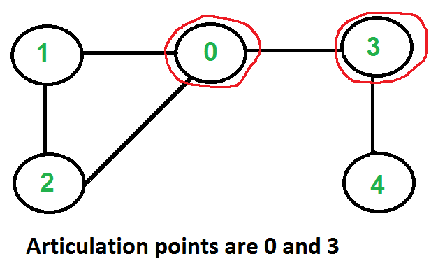

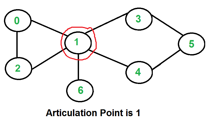
## References
- [GeeksForGeeks](https://www.geeksforgeeks.org/articulation-points-or-cut-vertices-in-a-graph/)
- [YouTube](https://www.youtube.com/watch?v=2kREIkF9UAs&list=PLLXdhg_r2hKA7DPDsunoDZ-Z769jWn4R8)
================================================
FILE: src/algorithms/graph/articulation-points/__test__/articulationPoints.test.js
================================================
import GraphVertex from '../../../../data-structures/graph/GraphVertex';
import GraphEdge from '../../../../data-structures/graph/GraphEdge';
import Graph from '../../../../data-structures/graph/Graph';
import articulationPoints from '../articulationPoints';
describe('articulationPoints', () => {
it('should find articulation points in simple graph', () => {
const vertexA = new GraphVertex('A');
const vertexB = new GraphVertex('B');
const vertexC = new GraphVertex('C');
const vertexD = new GraphVertex('D');
const edgeAB = new GraphEdge(vertexA, vertexB);
const edgeBC = new GraphEdge(vertexB, vertexC);
const edgeCD = new GraphEdge(vertexC, vertexD);
const graph = new Graph();
graph
.addEdge(edgeAB)
.addEdge(edgeBC)
.addEdge(edgeCD);
const articulationPointsSet = Object.values(articulationPoints(graph));
expect(articulationPointsSet.length).toBe(2);
expect(articulationPointsSet[0].getKey()).toBe(vertexC.getKey());
expect(articulationPointsSet[1].getKey()).toBe(vertexB.getKey());
});
it('should find articulation points in simple graph with back edge', () => {
const vertexA = new GraphVertex('A');
const vertexB = new GraphVertex('B');
const vertexC = new GraphVertex('C');
const vertexD = new GraphVertex('D');
const edgeAB = new GraphEdge(vertexA, vertexB);
const edgeBC = new GraphEdge(vertexB, vertexC);
const edgeCD = new GraphEdge(vertexC, vertexD);
const edgeAC = new GraphEdge(vertexA, vertexC);
const graph = new Graph();
graph
.addEdge(edgeAB)
.addEdge(edgeAC)
.addEdge(edgeBC)
.addEdge(edgeCD);
const articulationPointsSet = Object.values(articulationPoints(graph));
expect(articulationPointsSet.length).toBe(1);
expect(articulationPointsSet[0].getKey()).toBe(vertexC.getKey());
});
it('should find articulation points in simple graph with back edge #2', () => {
const vertexA = new GraphVertex('A');
const vertexB = new GraphVertex('B');
const vertexC = new GraphVertex('C');
const vertexD = new GraphVertex('D');
const vertexE = new GraphVertex('E');
const edgeAB = new GraphEdge(vertexA, vertexB);
const edgeBC = new GraphEdge(vertexB, vertexC);
const edgeCD = new GraphEdge(vertexC, vertexD);
const edgeAE = new GraphEdge(vertexA, vertexE);
const edgeCE = new GraphEdge(vertexC, vertexE);
const graph = new Graph();
graph
.addEdge(edgeAB)
.addEdge(edgeAE)
.addEdge(edgeCE)
.addEdge(edgeBC)
.addEdge(edgeCD);
const articulationPointsSet = Object.values(articulationPoints(graph));
expect(articulationPointsSet.length).toBe(1);
expect(articulationPointsSet[0].getKey()).toBe(vertexC.getKey());
});
it('should find articulation points in graph', () => {
const vertexA = new GraphVertex('A');
const vertexB = new GraphVertex('B');
const vertexC = new GraphVertex('C');
const vertexD = new GraphVertex('D');
const vertexE = new GraphVertex('E');
const vertexF = new GraphVertex('F');
const vertexG = new GraphVertex('G');
const vertexH = new GraphVertex('H');
const edgeAB = new GraphEdge(vertexA, vertexB);
const edgeBC = new GraphEdge(vertexB, vertexC);
const edgeAC = new GraphEdge(vertexA, vertexC);
const edgeCD = new GraphEdge(vertexC, vertexD);
const edgeDE = new GraphEdge(vertexD, vertexE);
const edgeEG = new GraphEdge(vertexE, vertexG);
const edgeEF = new GraphEdge(vertexE, vertexF);
const edgeGF = new GraphEdge(vertexG, vertexF);
const edgeFH = new GraphEdge(vertexF, vertexH);
const graph = new Graph();
graph
.addEdge(edgeAB)
.addEdge(edgeBC)
.addEdge(edgeAC)
.addEdge(edgeCD)
.addEdge(edgeDE)
.addEdge(edgeEG)
.addEdge(edgeEF)
.addEdge(edgeGF)
.addEdge(edgeFH);
const articulationPointsSet = Object.values(articulationPoints(graph));
expect(articulationPointsSet.length).toBe(4);
expect(articulationPointsSet[0].getKey()).toBe(vertexF.getKey());
expect(articulationPointsSet[1].getKey()).toBe(vertexE.getKey());
expect(articulationPointsSet[2].getKey()).toBe(vertexD.getKey());
expect(articulationPointsSet[3].getKey()).toBe(vertexC.getKey());
});
it('should find articulation points in graph starting with articulation root vertex', () => {
const vertexA = new GraphVertex('A');
const vertexB = new GraphVertex('B');
const vertexC = new GraphVertex('C');
const vertexD = new GraphVertex('D');
const vertexE = new GraphVertex('E');
const vertexF = new GraphVertex('F');
const vertexG = new GraphVertex('G');
const vertexH = new GraphVertex('H');
const edgeAB = new GraphEdge(vertexA, vertexB);
const edgeBC = new GraphEdge(vertexB, vertexC);
const edgeAC = new GraphEdge(vertexA, vertexC);
const edgeCD = new GraphEdge(vertexC, vertexD);
const edgeDE = new GraphEdge(vertexD, vertexE);
const edgeEG = new GraphEdge(vertexE, vertexG);
const edgeEF = new GraphEdge(vertexE, vertexF);
const edgeGF = new GraphEdge(vertexG, vertexF);
const edgeFH = new GraphEdge(vertexF, vertexH);
const graph = new Graph();
graph
.addEdge(edgeDE)
.addEdge(edgeAB)
.addEdge(edgeBC)
.addEdge(edgeAC)
.addEdge(edgeCD)
.addEdge(edgeEG)
.addEdge(edgeEF)
.addEdge(edgeGF)
.addEdge(edgeFH);
const articulationPointsSet = Object.values(articulationPoints(graph));
expect(articulationPointsSet.length).toBe(4);
expect(articulationPointsSet[0].getKey()).toBe(vertexF.getKey());
expect(articulationPointsSet[1].getKey()).toBe(vertexE.getKey());
expect(articulationPointsSet[2].getKey()).toBe(vertexC.getKey());
expect(articulationPointsSet[3].getKey()).toBe(vertexD.getKey());
});
it('should find articulation points in yet another graph #1', () => {
const vertexA = new GraphVertex('A');
const vertexB = new GraphVertex('B');
const vertexC = new GraphVertex('C');
const vertexD = new GraphVertex('D');
const vertexE = new GraphVertex('E');
const edgeAB = new GraphEdge(vertexA, vertexB);
const edgeAC = new GraphEdge(vertexA, vertexC);
const edgeBC = new GraphEdge(vertexB, vertexC);
const edgeCD = new GraphEdge(vertexC, vertexD);
const edgeDE = new GraphEdge(vertexD, vertexE);
const graph = new Graph();
graph
.addEdge(edgeAB)
.addEdge(edgeAC)
.addEdge(edgeBC)
.addEdge(edgeCD)
.addEdge(edgeDE);
const articulationPointsSet = Object.values(articulationPoints(graph));
expect(articulationPointsSet.length).toBe(2);
expect(articulationPointsSet[0].getKey()).toBe(vertexD.getKey());
expect(articulationPointsSet[1].getKey()).toBe(vertexC.getKey());
});
it('should find articulation points in yet another graph #2', () => {
const vertexA = new GraphVertex('A');
const vertexB = new GraphVertex('B');
const vertexC = new GraphVertex('C');
const vertexD = new GraphVertex('D');
const vertexE = new GraphVertex('E');
const vertexF = new GraphVertex('F');
const vertexG = new GraphVertex('G');
const edgeAB = new GraphEdge(vertexA, vertexB);
const edgeAC = new GraphEdge(vertexA, vertexC);
const edgeBC = new GraphEdge(vertexB, vertexC);
const edgeCD = new GraphEdge(vertexC, vertexD);
const edgeCE = new GraphEdge(vertexC, vertexE);
const edgeCF = new GraphEdge(vertexC, vertexF);
const edgeEG = new GraphEdge(vertexE, vertexG);
const edgeFG = new GraphEdge(vertexF, vertexG);
const graph = new Graph();
graph
.addEdge(edgeAB)
.addEdge(edgeAC)
.addEdge(edgeBC)
.addEdge(edgeCD)
.addEdge(edgeCE)
.addEdge(edgeCF)
.addEdge(edgeEG)
.addEdge(edgeFG);
const articulationPointsSet = Object.values(articulationPoints(graph));
expect(articulationPointsSet.length).toBe(1);
expect(articulationPointsSet[0].getKey()).toBe(vertexC.getKey());
});
});
================================================
FILE: src/algorithms/graph/articulation-points/articulationPoints.js
================================================
import depthFirstSearch from '../depth-first-search/depthFirstSearch';
/**
* Helper class for visited vertex metadata.
*/
class VisitMetadata {
constructor({ discoveryTime, lowDiscoveryTime }) {
this.discoveryTime = discoveryTime;
this.lowDiscoveryTime = lowDiscoveryTime;
// We need this in order to check graph root node, whether it has two
// disconnected children or not.
this.independentChildrenCount = 0;
}
}
/**
* Tarjan's algorithm for finding articulation points in graph.
*
* @param {Graph} graph
* @return {Object}
*/
export default function articulationPoints(graph) {
// Set of vertices we've already visited during DFS.
const visitedSet = {};
// Set of articulation points.
const articulationPointsSet = {};
// Time needed to discover to the current vertex.
let discoveryTime = 0;
// Peek the start vertex for DFS traversal.
const startVertex = graph.getAllVertices()[0];
const dfsCallbacks = {
/**
* @param {GraphVertex} currentVertex
* @param {GraphVertex} previousVertex
*/
enterVertex: ({ currentVertex, previousVertex }) => {
// Tick discovery time.
discoveryTime += 1;
// Put current vertex to visited set.
visitedSet[currentVertex.getKey()] = new VisitMetadata({
discoveryTime,
lowDiscoveryTime: discoveryTime,
});
if (previousVertex) {
// Update children counter for previous vertex.
visitedSet[previousVertex.getKey()].independentChildrenCount += 1;
}
},
/**
* @param {GraphVertex} currentVertex
* @param {GraphVertex} previousVertex
*/
leaveVertex: ({ currentVertex, previousVertex }) => {
if (previousVertex === null) {
// Don't do anything for the root vertex if it is already current (not previous one)
return;
}
// Update the low time with the smallest time of adjacent vertices.
// Get minimum low discovery time from all neighbors.
/** @param {GraphVertex} neighbor */
visitedSet[currentVertex.getKey()].lowDiscoveryTime = currentVertex.getNeighbors()
.filter((earlyNeighbor) => earlyNeighbor.getKey() !== previousVertex.getKey())
/**
* @param {number} lowestDiscoveryTime
* @param {GraphVertex} neighbor
*/
.reduce(
(lowestDiscoveryTime, neighbor) => {
const neighborLowTime = visitedSet[neighbor.getKey()].lowDiscoveryTime;
return neighborLowTime < lowestDiscoveryTime ? neighborLowTime : lowestDiscoveryTime;
},
visitedSet[currentVertex.getKey()].lowDiscoveryTime,
);
// Detect whether previous vertex is articulation point or not.
// To do so we need to check two [OR] conditions:
// 1. Is it a root vertex with at least two independent children.
// 2. If its visited time is <= low time of adjacent vertex.
if (previousVertex === startVertex) {
// Check that root vertex has at least two independent children.
if (visitedSet[previousVertex.getKey()].independentChildrenCount >= 2) {
articulationPointsSet[previousVertex.getKey()] = previousVertex;
}
} else {
// Get current vertex low discovery time.
const currentLowDiscoveryTime = visitedSet[currentVertex.getKey()].lowDiscoveryTime;
// Compare current vertex low discovery time with parent discovery time. Check if there
// are any short path (back edge) exists. If we can't get to current vertex other then
// via parent then the parent vertex is articulation point for current one.
const parentDiscoveryTime = visitedSet[previousVertex.getKey()].discoveryTime;
if (parentDiscoveryTime <= currentLowDiscoveryTime) {
articulationPointsSet[previousVertex.getKey()] = previousVertex;
}
}
},
allowTraversal: ({ nextVertex }) => {
return !visitedSet[nextVertex.getKey()];
},
};
// Do Depth First Search traversal over submitted graph.
depthFirstSearch(graph, startVertex, dfsCallbacks);
return articulationPointsSet;
}
================================================
FILE: src/algorithms/graph/bellman-ford/README.md
================================================
# Bellman–Ford Algorithm
The Bellman–Ford algorithm is an algorithm that computes shortest
paths from a single source vertex to all of the other vertices
in a weighted digraph. It is slower than Dijkstra's algorithm
for the same problem, but more versatile, as it is capable of
handling graphs in which some of the edge weights are negative
numbers.

## Complexity
Worst-case performance `O(|V||E|)`
Best-case performance `O(|E|)`
Worst-case space complexity `O(|V|)`
## References
- [Wikipedia](https://en.wikipedia.org/wiki/Bellman%E2%80%93Ford_algorithm)
- [On YouTube by Michael Sambol](https://www.youtube.com/watch?v=obWXjtg0L64&list=PLLXdhg_r2hKA7DPDsunoDZ-Z769jWn4R8)
================================================
FILE: src/algorithms/graph/bellman-ford/__test__/bellmanFord.test.js
================================================
import GraphVertex from '../../../../data-structures/graph/GraphVertex';
import GraphEdge from '../../../../data-structures/graph/GraphEdge';
import Graph from '../../../../data-structures/graph/Graph';
import bellmanFord from '../bellmanFord';
describe('bellmanFord', () => {
it('should find minimum paths to all vertices for undirected graph', () => {
const vertexA = new GraphVertex('A');
const vertexB = new GraphVertex('B');
const vertexC = new GraphVertex('C');
const vertexD = new GraphVertex('D');
const vertexE = new GraphVertex('E');
const vertexF = new GraphVertex('F');
const vertexG = new GraphVertex('G');
const vertexH = new GraphVertex('H');
const edgeAB = new GraphEdge(vertexA, vertexB, 4);
const edgeAE = new GraphEdge(vertexA, vertexE, 7);
const edgeAC = new GraphEdge(vertexA, vertexC, 3);
const edgeBC = new GraphEdge(vertexB, vertexC, 6);
const edgeBD = new GraphEdge(vertexB, vertexD, 5);
const edgeEC = new GraphEdge(vertexE, vertexC, 8);
const edgeED = new GraphEdge(vertexE, vertexD, 2);
const edgeDC = new GraphEdge(vertexD, vertexC, 11);
const edgeDG = new GraphEdge(vertexD, vertexG, 10);
const edgeDF = new GraphEdge(vertexD, vertexF, 2);
const edgeFG = new GraphEdge(vertexF, vertexG, 3);
const edgeEG = new GraphEdge(vertexE, vertexG, 5);
const graph = new Graph();
graph
.addVertex(vertexH)
.addEdge(edgeAB)
.addEdge(edgeAE)
.addEdge(edgeAC)
.addEdge(edgeBC)
.addEdge(edgeBD)
.addEdge(edgeEC)
.addEdge(edgeED)
.addEdge(edgeDC)
.addEdge(edgeDG)
.addEdge(edgeDF)
.addEdge(edgeFG)
.addEdge(edgeEG);
const { distances, previousVertices } = bellmanFord(graph, vertexA);
expect(distances).toEqual({
H: Infinity,
A: 0,
B: 4,
E: 7,
C: 3,
D: 9,
G: 12,
F: 11,
});
expect(previousVertices.F.getKey()).toBe('D');
expect(previousVertices.D.getKey()).toBe('B');
expect(previousVertices.B.getKey()).toBe('A');
expect(previousVertices.G.getKey()).toBe('E');
expect(previousVertices.C.getKey()).toBe('A');
expect(previousVertices.A).toBeNull();
expect(previousVertices.H).toBeNull();
});
it('should find minimum paths to all vertices for directed graph with negative edge weights', () => {
const vertexS = new GraphVertex('S');
const vertexE = new GraphVertex('E');
const vertexA = new GraphVertex('A');
const vertexD = new GraphVertex('D');
const vertexB = new GraphVertex('B');
const vertexC = new GraphVertex('C');
const vertexH = new GraphVertex('H');
const edgeSE = new GraphEdge(vertexS, vertexE, 8);
const edgeSA = new GraphEdge(vertexS, vertexA, 10);
const edgeED = new GraphEdge(vertexE, vertexD, 1);
const edgeDA = new GraphEdge(vertexD, vertexA, -4);
const edgeDC = new GraphEdge(vertexD, vertexC, -1);
const edgeAC = new GraphEdge(vertexA, vertexC, 2);
const edgeCB = new GraphEdge(vertexC, vertexB, -2);
const edgeBA = new GraphEdge(vertexB, vertexA, 1);
const graph = new Graph(true);
graph
.addVertex(vertexH)
.addEdge(edgeSE)
.addEdge(edgeSA)
.addEdge(edgeED)
.addEdge(edgeDA)
.addEdge(edgeDC)
.addEdge(edgeAC)
.addEdge(edgeCB)
.addEdge(edgeBA);
const { distances, previousVertices } = bellmanFord(graph, vertexS);
expect(distances).toEqual({
H: Infinity,
S: 0,
A: 5,
B: 5,
C: 7,
D: 9,
E: 8,
});
expect(previousVertices.H).toBeNull();
expect(previousVertices.S).toBeNull();
expect(previousVertices.B.getKey()).toBe('C');
expect(previousVertices.C.getKey()).toBe('A');
expect(previousVertices.A.getKey()).toBe('D');
expect(previousVertices.D.getKey()).toBe('E');
});
});
================================================
FILE: src/algorithms/graph/bellman-ford/bellmanFord.js
================================================
/**
* @param {Graph} graph
* @param {GraphVertex} startVertex
* @return {{distances, previousVertices}}
*/
export default function bellmanFord(graph, startVertex) {
const distances = {};
const previousVertices = {};
// Init all distances with infinity assuming that currently we can't reach
// any of the vertices except start one.
distances[startVertex.getKey()] = 0;
graph.getAllVertices().forEach((vertex) => {
previousVertices[vertex.getKey()] = null;
if (vertex.getKey() !== startVertex.getKey()) {
distances[vertex.getKey()] = Infinity;
}
});
// We need (|V| - 1) iterations.
for (let iteration = 0; iteration < (graph.getAllVertices().length - 1); iteration += 1) {
// During each iteration go through all vertices.
Object.keys(distances).forEach((vertexKey) => {
const vertex = graph.getVertexByKey(vertexKey);
// Go through all vertex edges.
graph.getNeighbors(vertex).forEach((neighbor) => {
const edge = graph.findEdge(vertex, neighbor);
// Find out if the distance to the neighbor is shorter in this iteration
// then in previous one.
const distanceToVertex = distances[vertex.getKey()];
const distanceToNeighbor = distanceToVertex + edge.weight;
if (distanceToNeighbor < distances[neighbor.getKey()]) {
distances[neighbor.getKey()] = distanceToNeighbor;
previousVertices[neighbor.getKey()] = vertex;
}
});
});
}
return {
distances,
previousVertices,
};
}
================================================
FILE: src/algorithms/graph/breadth-first-search/README.md
================================================
# Breadth-First Search (BFS)
Breadth-first search (BFS) is an algorithm for traversing,
searching tree, or graph data structures. It starts at
the tree root (or some arbitrary node of a graph, sometimes
referred to as a 'search key') and explores the neighbor
nodes first, before moving to the next level neighbors.
## References
- [Wikipedia](https://en.wikipedia.org/wiki/Breadth-first_search)
- [Tree Traversals (Inorder, Preorder and Postorder)](https://www.geeksforgeeks.org/tree-traversals-inorder-preorder-and-postorder/)
- [BFS vs DFS](https://www.geeksforgeeks.org/bfs-vs-dfs-binary-tree/)
- [BFS Visualization](https://www.cs.usfca.edu/~galles/visualization/BFS.html)
================================================
FILE: src/algorithms/graph/breadth-first-search/__test__/breadthFirstSearch.test.js
================================================
import Graph from '../../../../data-structures/graph/Graph';
import GraphVertex from '../../../../data-structures/graph/GraphVertex';
import GraphEdge from '../../../../data-structures/graph/GraphEdge';
import breadthFirstSearch from '../breadthFirstSearch';
describe('breadthFirstSearch', () => {
it('should perform BFS operation on graph', () => {
const graph = new Graph(true);
const vertexA = new GraphVertex('A');
const vertexB = new GraphVertex('B');
const vertexC = new GraphVertex('C');
const vertexD = new GraphVertex('D');
const vertexE = new GraphVertex('E');
const vertexF = new GraphVertex('F');
const vertexG = new GraphVertex('G');
const vertexH = new GraphVertex('H');
const edgeAB = new GraphEdge(vertexA, vertexB);
const edgeBC = new GraphEdge(vertexB, vertexC);
const edgeCG = new GraphEdge(vertexC, vertexG);
const edgeAD = new GraphEdge(vertexA, vertexD);
const edgeAE = new GraphEdge(vertexA, vertexE);
const edgeEF = new GraphEdge(vertexE, vertexF);
const edgeFD = new GraphEdge(vertexF, vertexD);
const edgeDH = new GraphEdge(vertexD, vertexH);
const edgeGH = new GraphEdge(vertexG, vertexH);
graph
.addEdge(edgeAB)
.addEdge(edgeBC)
.addEdge(edgeCG)
.addEdge(edgeAD)
.addEdge(edgeAE)
.addEdge(edgeEF)
.addEdge(edgeFD)
.addEdge(edgeDH)
.addEdge(edgeGH);
expect(graph.toString()).toBe('A,B,C,G,D,E,F,H');
const enterVertexCallback = jest.fn();
const leaveVertexCallback = jest.fn();
// Traverse graphs without callbacks first.
breadthFirstSearch(graph, vertexA);
// Traverse graph with enterVertex and leaveVertex callbacks.
breadthFirstSearch(graph, vertexA, {
enterVertex: enterVertexCallback,
leaveVertex: leaveVertexCallback,
});
expect(enterVertexCallback).toHaveBeenCalledTimes(8);
expect(leaveVertexCallback).toHaveBeenCalledTimes(8);
const enterVertexParamsMap = [
{ currentVertex: vertexA, previousVertex: null },
{ currentVertex: vertexB, previousVertex: vertexA },
{ currentVertex: vertexD, previousVertex: vertexB },
{ currentVertex: vertexE, previousVertex: vertexD },
{ currentVertex: vertexC, previousVertex: vertexE },
{ currentVertex: vertexH, previousVertex: vertexC },
{ currentVertex: vertexF, previousVertex: vertexH },
{ currentVertex: vertexG, previousVertex: vertexF },
];
for (let callIndex = 0; callIndex < graph.getAllVertices().length; callIndex += 1) {
const params = enterVertexCallback.mock.calls[callIndex][0];
expect(params.currentVertex).toEqual(enterVertexParamsMap[callIndex].currentVertex);
expect(params.previousVertex).toEqual(enterVertexParamsMap[callIndex].previousVertex);
}
const leaveVertexParamsMap = [
{ currentVertex: vertexA, previousVertex: null },
{ currentVertex: vertexB, previousVertex: vertexA },
{ currentVertex: vertexD, previousVertex: vertexB },
{ currentVertex: vertexE, previousVertex: vertexD },
{ currentVertex: vertexC, previousVertex: vertexE },
{ currentVertex: vertexH, previousVertex: vertexC },
{ currentVertex: vertexF, previousVertex: vertexH },
{ currentVertex: vertexG, previousVertex: vertexF },
];
for (let callIndex = 0; callIndex < graph.getAllVertices().length; callIndex += 1) {
const params = leaveVertexCallback.mock.calls[callIndex][0];
expect(params.currentVertex).toEqual(leaveVertexParamsMap[callIndex].currentVertex);
expect(params.previousVertex).toEqual(leaveVertexParamsMap[callIndex].previousVertex);
}
});
it('should allow to create custom vertex visiting logic', () => {
const graph = new Graph(true);
const vertexA = new GraphVertex('A');
const vertexB = new GraphVertex('B');
const vertexC = new GraphVertex('C');
const vertexD = new GraphVertex('D');
const vertexE = new GraphVertex('E');
const vertexF = new GraphVertex('F');
const vertexG = new GraphVertex('G');
const vertexH = new GraphVertex('H');
const edgeAB = new GraphEdge(vertexA, vertexB);
const edgeBC = new GraphEdge(vertexB, vertexC);
const edgeCG = new GraphEdge(vertexC, vertexG);
const edgeAD = new GraphEdge(vertexA, vertexD);
const edgeAE = new GraphEdge(vertexA, vertexE);
const edgeEF = new GraphEdge(vertexE, vertexF);
const edgeFD = new GraphEdge(vertexF, vertexD);
const edgeDH = new GraphEdge(vertexD, vertexH);
const edgeGH = new GraphEdge(vertexG, vertexH);
graph
.addEdge(edgeAB)
.addEdge(edgeBC)
.addEdge(edgeCG)
.addEdge(edgeAD)
.addEdge(edgeAE)
.addEdge(edgeEF)
.addEdge(edgeFD)
.addEdge(edgeDH)
.addEdge(edgeGH);
expect(graph.toString()).toBe('A,B,C,G,D,E,F,H');
const enterVertexCallback = jest.fn();
const leaveVertexCallback = jest.fn();
// Traverse graph with enterVertex and leaveVertex callbacks.
breadthFirstSearch(graph, vertexA, {
enterVertex: enterVertexCallback,
leaveVertex: leaveVertexCallback,
allowTraversal: ({ currentVertex, nextVertex }) => {
return !(currentVertex === vertexA && nextVertex === vertexB);
},
});
expect(enterVertexCallback).toHaveBeenCalledTimes(7);
expect(leaveVertexCallback).toHaveBeenCalledTimes(7);
const enterVertexParamsMap = [
{ currentVertex: vertexA, previousVertex: null },
{ currentVertex: vertexD, previousVertex: vertexA },
{ currentVertex: vertexE, previousVertex: vertexD },
{ currentVertex: vertexH, previousVertex: vertexE },
{ currentVertex: vertexF, previousVertex: vertexH },
{ currentVertex: vertexD, previousVertex: vertexF },
{ currentVertex: vertexH, previousVertex: vertexD },
];
for (let callIndex = 0; callIndex < 7; callIndex += 1) {
const params = enterVertexCallback.mock.calls[callIndex][0];
expect(params.currentVertex).toEqual(enterVertexParamsMap[callIndex].currentVertex);
expect(params.previousVertex).toEqual(enterVertexParamsMap[callIndex].previousVertex);
}
const leaveVertexParamsMap = [
{ currentVertex: vertexA, previousVertex: null },
{ currentVertex: vertexD, previousVertex: vertexA },
{ currentVertex: vertexE, previousVertex: vertexD },
{ currentVertex: vertexH, previousVertex: vertexE },
{ currentVertex: vertexF, previousVertex: vertexH },
{ currentVertex: vertexD, previousVertex: vertexF },
{ currentVertex: vertexH, previousVertex: vertexD },
];
for (let callIndex = 0; callIndex < 7; callIndex += 1) {
const params = leaveVertexCallback.mock.calls[callIndex][0];
expect(params.currentVertex).toEqual(leaveVertexParamsMap[callIndex].currentVertex);
expect(params.previousVertex).toEqual(leaveVertexParamsMap[callIndex].previousVertex);
}
});
});
================================================
FILE: src/algorithms/graph/breadth-first-search/breadthFirstSearch.js
================================================
import Queue from '../../../data-structures/queue/Queue';
/**
* @typedef {Object} Callbacks
*
* @property {function(vertices: Object): boolean} [allowTraversal] -
* Determines whether DFS should traverse from the vertex to its neighbor
* (along the edge). By default prohibits visiting the same vertex again.
*
* @property {function(vertices: Object)} [enterVertex] - Called when BFS enters the vertex.
*
* @property {function(vertices: Object)} [leaveVertex] - Called when BFS leaves the vertex.
*/
/**
* @param {Callbacks} [callbacks]
* @returns {Callbacks}
*/
function initCallbacks(callbacks = {}) {
const initiatedCallback = callbacks;
const stubCallback = () => {};
const allowTraversalCallback = (
() => {
const seen = {};
return ({ nextVertex }) => {
if (!seen[nextVertex.getKey()]) {
seen[nextVertex.getKey()] = true;
return true;
}
return false;
};
}
)();
initiatedCallback.allowTraversal = callbacks.allowTraversal || allowTraversalCallback;
initiatedCallback.enterVertex = callbacks.enterVertex || stubCallback;
initiatedCallback.leaveVertex = callbacks.leaveVertex || stubCallback;
return initiatedCallback;
}
/**
* @param {Graph} graph
* @param {GraphVertex} startVertex
* @param {Callbacks} [originalCallbacks]
*/
export default function breadthFirstSearch(graph, startVertex, originalCallbacks) {
const callbacks = initCallbacks(originalCallbacks);
const vertexQueue = new Queue();
// Do initial queue setup.
vertexQueue.enqueue(startVertex);
let previousVertex = null;
// Traverse all vertices from the queue.
while (!vertexQueue.isEmpty()) {
const currentVertex = vertexQueue.dequeue();
callbacks.enterVertex({ currentVertex, previousVertex });
// Add all neighbors to the queue for future traversals.
graph.getNeighbors(currentVertex).forEach((nextVertex) => {
if (callbacks.allowTraversal({ previousVertex, currentVertex, nextVertex })) {
vertexQueue.enqueue(nextVertex);
}
});
callbacks.leaveVertex({ currentVertex, previousVertex });
// Memorize current vertex before next loop.
previousVertex = currentVertex;
}
}
================================================
FILE: src/algorithms/graph/bridges/README.md
================================================
# Bridges in Graph
In graph theory, a **bridge**, **isthmus**, **cut-edge**, or **cut arc** is an edge
of a graph whose deletion increases its number of connected components. Equivalently,
an edge is a bridge if and only if it is not contained in any cycle. A graph is said
to be bridgeless or isthmus-free if it contains no bridges.

A graph with 16 vertices and 6 bridges (highlighted in red)

An undirected connected graph with no cut edges

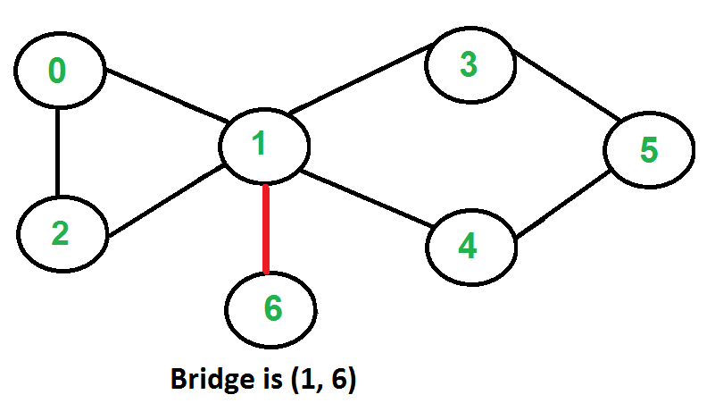
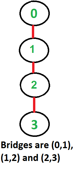
## References
- [GeeksForGeeks on YouTube](https://www.youtube.com/watch?v=thLQYBlz2DM&list=PLLXdhg_r2hKA7DPDsunoDZ-Z769jWn4R8)
- [Wikipedia](https://en.wikipedia.org/wiki/Bridge_%28graph_theory%29#Tarjan.27s_Bridge-finding_algorithm)
- [GeeksForGeeks](https://www.geeksforgeeks.org/bridge-in-a-graph/)
================================================
FILE: src/algorithms/graph/bridges/__test__/graphBridges.test.js
================================================
import GraphVertex from '../../../../data-structures/graph/GraphVertex';
import GraphEdge from '../../../../data-structures/graph/GraphEdge';
import Graph from '../../../../data-structures/graph/Graph';
import graphBridges from '../graphBridges';
describe('graphBridges', () => {
it('should find bridges in simple graph', () => {
const vertexA = new GraphVertex('A');
const vertexB = new GraphVertex('B');
const vertexC = new GraphVertex('C');
const vertexD = new GraphVertex('D');
const edgeAB = new GraphEdge(vertexA, vertexB);
const edgeBC = new GraphEdge(vertexB, vertexC);
const edgeCD = new GraphEdge(vertexC, vertexD);
const graph = new Graph();
graph
.addEdge(edgeAB)
.addEdge(edgeBC)
.addEdge(edgeCD);
const bridges = Object.values(graphBridges(graph));
expect(bridges.length).toBe(3);
expect(bridges[0].getKey()).toBe(edgeCD.getKey());
expect(bridges[1].getKey()).toBe(edgeBC.getKey());
expect(bridges[2].getKey()).toBe(edgeAB.getKey());
});
it('should find bridges in simple graph with back edge', () => {
const vertexA = new GraphVertex('A');
const vertexB = new GraphVertex('B');
const vertexC = new GraphVertex('C');
const vertexD = new GraphVertex('D');
const edgeAB = new GraphEdge(vertexA, vertexB);
const edgeBC = new GraphEdge(vertexB, vertexC);
const edgeCD = new GraphEdge(vertexC, vertexD);
const edgeAC = new GraphEdge(vertexA, vertexC);
const graph = new Graph();
graph
.addEdge(edgeAB)
.addEdge(edgeAC)
.addEdge(edgeBC)
.addEdge(edgeCD);
const bridges = Object.values(graphBridges(graph));
expect(bridges.length).toBe(1);
expect(bridges[0].getKey()).toBe(edgeCD.getKey());
});
it('should find bridges in graph', () => {
const vertexA = new GraphVertex('A');
const vertexB = new GraphVertex('B');
const vertexC = new GraphVertex('C');
const vertexD = new GraphVertex('D');
const vertexE = new GraphVertex('E');
const vertexF = new GraphVertex('F');
const vertexG = new GraphVertex('G');
const vertexH = new GraphVertex('H');
const edgeAB = new GraphEdge(vertexA, vertexB);
const edgeBC = new GraphEdge(vertexB, vertexC);
const edgeAC = new GraphEdge(vertexA, vertexC);
const edgeCD = new GraphEdge(vertexC, vertexD);
const edgeDE = new GraphEdge(vertexD, vertexE);
const edgeEG = new GraphEdge(vertexE, vertexG);
const edgeEF = new GraphEdge(vertexE, vertexF);
const edgeGF = new GraphEdge(vertexG, vertexF);
const edgeFH = new GraphEdge(vertexF, vertexH);
const graph = new Graph();
graph
.addEdge(edgeAB)
.addEdge(edgeBC)
.addEdge(edgeAC)
.addEdge(edgeCD)
.addEdge(edgeDE)
.addEdge(edgeEG)
.addEdge(edgeEF)
.addEdge(edgeGF)
.addEdge(edgeFH);
const bridges = Object.values(graphBridges(graph));
expect(bridges.length).toBe(3);
expect(bridges[0].getKey()).toBe(edgeFH.getKey());
expect(bridges[1].getKey()).toBe(edgeDE.getKey());
expect(bridges[2].getKey()).toBe(edgeCD.getKey());
});
it('should find bridges in graph starting with different root vertex', () => {
const vertexA = new GraphVertex('A');
const vertexB = new GraphVertex('B');
const vertexC = new GraphVertex('C');
const vertexD = new GraphVertex('D');
const vertexE = new GraphVertex('E');
const vertexF = new GraphVertex('F');
const vertexG = new GraphVertex('G');
const vertexH = new GraphVertex('H');
const edgeAB = new GraphEdge(vertexA, vertexB);
const edgeBC = new GraphEdge(vertexB, vertexC);
const edgeAC = new GraphEdge(vertexA, vertexC);
const edgeCD = new GraphEdge(vertexC, vertexD);
const edgeDE = new GraphEdge(vertexD, vertexE);
const edgeEG = new GraphEdge(vertexE, vertexG);
const edgeEF = new GraphEdge(vertexE, vertexF);
const edgeGF = new GraphEdge(vertexG, vertexF);
const edgeFH = new GraphEdge(vertexF, vertexH);
const graph = new Graph();
graph
.addEdge(edgeDE)
.addEdge(edgeAB)
.addEdge(edgeBC)
.addEdge(edgeAC)
.addEdge(edgeCD)
.addEdge(edgeEG)
.addEdge(edgeEF)
.addEdge(edgeGF)
.addEdge(edgeFH);
const bridges = Object.values(graphBridges(graph));
expect(bridges.length).toBe(3);
expect(bridges[0].getKey()).toBe(edgeFH.getKey());
expect(bridges[1].getKey()).toBe(edgeDE.getKey());
expect(bridges[2].getKey()).toBe(edgeCD.getKey());
});
it('should find bridges in yet another graph #1', () => {
const vertexA = new GraphVertex('A');
const vertexB = new GraphVertex('B');
const vertexC = new GraphVertex('C');
const vertexD = new GraphVertex('D');
const vertexE = new GraphVertex('E');
const edgeAB = new GraphEdge(vertexA, vertexB);
const edgeAC = new GraphEdge(vertexA, vertexC);
const edgeBC = new GraphEdge(vertexB, vertexC);
const edgeCD = new GraphEdge(vertexC, vertexD);
const edgeDE = new GraphEdge(vertexD, vertexE);
const graph = new Graph();
graph
.addEdge(edgeAB)
.addEdge(edgeAC)
.addEdge(edgeBC)
.addEdge(edgeCD)
.addEdge(edgeDE);
const bridges = Object.values(graphBridges(graph));
expect(bridges.length).toBe(2);
expect(bridges[0].getKey()).toBe(edgeDE.getKey());
expect(bridges[1].getKey()).toBe(edgeCD.getKey());
});
it('should find bridges in yet another graph #2', () => {
const vertexA = new GraphVertex('A');
const vertexB = new GraphVertex('B');
const vertexC = new GraphVertex('C');
const vertexD = new GraphVertex('D');
const vertexE = new GraphVertex('E');
const vertexF = new GraphVertex('F');
const vertexG = new GraphVertex('G');
const edgeAB = new GraphEdge(vertexA, vertexB);
const edgeAC = new GraphEdge(vertexA, vertexC);
const edgeBC = new GraphEdge(vertexB, vertexC);
const edgeCD = new GraphEdge(vertexC, vertexD);
const edgeCE = new GraphEdge(vertexC, vertexE);
const edgeCF = new GraphEdge(vertexC, vertexF);
const edgeEG = new GraphEdge(vertexE, vertexG);
const edgeFG = new GraphEdge(vertexF, vertexG);
const graph = new Graph();
graph
.addEdge(edgeAB)
.addEdge(edgeAC)
.addEdge(edgeBC)
.addEdge(edgeCD)
.addEdge(edgeCE)
.addEdge(edgeCF)
.addEdge(edgeEG)
.addEdge(edgeFG);
const bridges = Object.values(graphBridges(graph));
expect(bridges.length).toBe(1);
expect(bridges[0].getKey()).toBe(edgeCD.getKey());
});
});
================================================
FILE: src/algorithms/graph/bridges/graphBridges.js
================================================
import depthFirstSearch from '../depth-first-search/depthFirstSearch';
/**
* Helper class for visited vertex metadata.
*/
class VisitMetadata {
constructor({ discoveryTime, lowDiscoveryTime }) {
this.discoveryTime = discoveryTime;
this.lowDiscoveryTime = lowDiscoveryTime;
}
}
/**
* @param {Graph} graph
* @return {Object}
*/
export default function graphBridges(graph) {
// Set of vertices we've already visited during DFS.
const visitedSet = {};
// Set of bridges.
const bridges = {};
// Time needed to discover to the current vertex.
let discoveryTime = 0;
// Peek the start vertex for DFS traversal.
const startVertex = graph.getAllVertices()[0];
const dfsCallbacks = {
/**
* @param {GraphVertex} currentVertex
*/
enterVertex: ({ currentVertex }) => {
// Tick discovery time.
discoveryTime += 1;
// Put current vertex to visited set.
visitedSet[currentVertex.getKey()] = new VisitMetadata({
discoveryTime,
lowDiscoveryTime: discoveryTime,
});
},
/**
* @param {GraphVertex} currentVertex
* @param {GraphVertex} previousVertex
*/
leaveVertex: ({ currentVertex, previousVertex }) => {
if (previousVertex === null) {
// Don't do anything for the root vertex if it is already current (not previous one).
return;
}
// Check if current node is connected to any early node other then previous one.
visitedSet[currentVertex.getKey()].lowDiscoveryTime = currentVertex.getNeighbors()
.filter((earlyNeighbor) => earlyNeighbor.getKey() !== previousVertex.getKey())
.reduce(
/**
* @param {number} lowestDiscoveryTime
* @param {GraphVertex} neighbor
*/
(lowestDiscoveryTime, neighbor) => {
const neighborLowTime = visitedSet[neighbor.getKey()].lowDiscoveryTime;
return neighborLowTime < lowestDiscoveryTime ? neighborLowTime : lowestDiscoveryTime;
},
visitedSet[currentVertex.getKey()].lowDiscoveryTime,
);
// Compare low discovery times. In case if current low discovery time is less than the one
// in previous vertex then update previous vertex low time.
const currentLowDiscoveryTime = visitedSet[currentVertex.getKey()].lowDiscoveryTime;
const previousLowDiscoveryTime = visitedSet[previousVertex.getKey()].lowDiscoveryTime;
if (currentLowDiscoveryTime < previousLowDiscoveryTime) {
visitedSet[previousVertex.getKey()].lowDiscoveryTime = currentLowDiscoveryTime;
}
// Compare current vertex low discovery time with parent discovery time. Check if there
// are any short path (back edge) exists. If we can't get to current vertex other then
// via parent then the parent vertex is articulation point for current one.
const parentDiscoveryTime = visitedSet[previousVertex.getKey()].discoveryTime;
if (parentDiscoveryTime < currentLowDiscoveryTime) {
const bridge = graph.findEdge(previousVertex, currentVertex);
bridges[bridge.getKey()] = bridge;
}
},
allowTraversal: ({ nextVertex }) => {
return !visitedSet[nextVertex.getKey()];
},
};
// Do Depth First Search traversal over submitted graph.
depthFirstSearch(graph, startVertex, dfsCallbacks);
return bridges;
}
================================================
FILE: src/algorithms/graph/depth-first-search/README.md
================================================
# Depth-First Search (DFS)
Depth-first search (DFS) is an algorithm for traversing or
searching tree or graph data structures. One starts at
the root (selecting some arbitrary node as the root in
the case of a graph) and explores as far as possible
along each branch before backtracking.

## References
- [Wikipedia](https://en.wikipedia.org/wiki/Depth-first_search)
- [Tree Traversals (Inorder, Preorder and Postorder)](https://www.geeksforgeeks.org/tree-traversals-inorder-preorder-and-postorder/)
- [BFS vs DFS](https://www.geeksforgeeks.org/bfs-vs-dfs-binary-tree/)
- [DFS Visualization](https://www.cs.usfca.edu/~galles/visualization/DFS.html)
================================================
FILE: src/algorithms/graph/depth-first-search/__test__/depthFirstSearch.test.js
================================================
import Graph from '../../../../data-structures/graph/Graph';
import GraphVertex from '../../../../data-structures/graph/GraphVertex';
import GraphEdge from '../../../../data-structures/graph/GraphEdge';
import depthFirstSearch from '../depthFirstSearch';
describe('depthFirstSearch', () => {
it('should perform DFS operation on graph', () => {
const graph = new Graph(true);
const vertexA = new GraphVertex('A');
const vertexB = new GraphVertex('B');
const vertexC = new GraphVertex('C');
const vertexD = new GraphVertex('D');
const vertexE = new GraphVertex('E');
const vertexF = new GraphVertex('F');
const vertexG = new GraphVertex('G');
const edgeAB = new GraphEdge(vertexA, vertexB);
const edgeBC = new GraphEdge(vertexB, vertexC);
const edgeCG = new GraphEdge(vertexC, vertexG);
const edgeAD = new GraphEdge(vertexA, vertexD);
const edgeAE = new GraphEdge(vertexA, vertexE);
const edgeEF = new GraphEdge(vertexE, vertexF);
const edgeFD = new GraphEdge(vertexF, vertexD);
const edgeDG = new GraphEdge(vertexD, vertexG);
graph
.addEdge(edgeAB)
.addEdge(edgeBC)
.addEdge(edgeCG)
.addEdge(edgeAD)
.addEdge(edgeAE)
.addEdge(edgeEF)
.addEdge(edgeFD)
.addEdge(edgeDG);
expect(graph.toString()).toBe('A,B,C,G,D,E,F');
const enterVertexCallback = jest.fn();
const leaveVertexCallback = jest.fn();
// Traverse graphs without callbacks first to check default ones.
depthFirstSearch(graph, vertexA);
// Traverse graph with enterVertex and leaveVertex callbacks.
depthFirstSearch(graph, vertexA, {
enterVertex: enterVertexCallback,
leaveVertex: leaveVertexCallback,
});
expect(enterVertexCallback).toHaveBeenCalledTimes(graph.getAllVertices().length);
expect(leaveVertexCallback).toHaveBeenCalledTimes(graph.getAllVertices().length);
const enterVertexParamsMap = [
{ currentVertex: vertexA, previousVertex: null },
{ currentVertex: vertexB, previousVertex: vertexA },
{ currentVertex: vertexC, previousVertex: vertexB },
{ currentVertex: vertexG, previousVertex: vertexC },
{ currentVertex: vertexD, previousVertex: vertexA },
{ currentVertex: vertexE, previousVertex: vertexA },
{ currentVertex: vertexF, previousVertex: vertexE },
];
for (let callIndex = 0; callIndex < graph.getAllVertices().length; callIndex += 1) {
const params = enterVertexCallback.mock.calls[callIndex][0];
expect(params.currentVertex).toEqual(enterVertexParamsMap[callIndex].currentVertex);
expect(params.previousVertex).toEqual(enterVertexParamsMap[callIndex].previousVertex);
}
const leaveVertexParamsMap = [
{ currentVertex: vertexG, previousVertex: vertexC },
{ currentVertex: vertexC, previousVertex: vertexB },
{ currentVertex: vertexB, previousVertex: vertexA },
{ currentVertex: vertexD, previousVertex: vertexA },
{ currentVertex: vertexF, previousVertex: vertexE },
{ currentVertex: vertexE, previousVertex: vertexA },
{ currentVertex: vertexA, previousVertex: null },
];
for (let callIndex = 0; callIndex < graph.getAllVertices().length; callIndex += 1) {
const params = leaveVertexCallback.mock.calls[callIndex][0];
expect(params.currentVertex).toEqual(leaveVertexParamsMap[callIndex].currentVertex);
expect(params.previousVertex).toEqual(leaveVertexParamsMap[callIndex].previousVertex);
}
});
it('allow users to redefine vertex visiting logic', () => {
const graph = new Graph(true);
const vertexA = new GraphVertex('A');
const vertexB = new GraphVertex('B');
const vertexC = new GraphVertex('C');
const vertexD = new GraphVertex('D');
const vertexE = new GraphVertex('E');
const vertexF = new GraphVertex('F');
const vertexG = new GraphVertex('G');
const edgeAB = new GraphEdge(vertexA, vertexB);
const edgeBC = new GraphEdge(vertexB, vertexC);
const edgeCG = new GraphEdge(vertexC, vertexG);
const edgeAD = new GraphEdge(vertexA, vertexD);
const edgeAE = new GraphEdge(vertexA, vertexE);
const edgeEF = new GraphEdge(vertexE, vertexF);
const edgeFD = new GraphEdge(vertexF, vertexD);
const edgeDG = new GraphEdge(vertexD, vertexG);
graph
.addEdge(edgeAB)
.addEdge(edgeBC)
.addEdge(edgeCG)
.addEdge(edgeAD)
.addEdge(edgeAE)
.addEdge(edgeEF)
.addEdge(edgeFD)
.addEdge(edgeDG);
expect(graph.toString()).toBe('A,B,C,G,D,E,F');
const enterVertexCallback = jest.fn();
const leaveVertexCallback = jest.fn();
depthFirstSearch(graph, vertexA, {
enterVertex: enterVertexCallback,
leaveVertex: leaveVertexCallback,
allowTraversal: ({ currentVertex, nextVertex }) => {
return !(currentVertex === vertexA && nextVertex === vertexB);
},
});
expect(enterVertexCallback).toHaveBeenCalledTimes(7);
expect(leaveVertexCallback).toHaveBeenCalledTimes(7);
const enterVertexParamsMap = [
{ currentVertex: vertexA, previousVertex: null },
{ currentVertex: vertexD, previousVertex: vertexA },
{ currentVertex: vertexG, previousVertex: vertexD },
{ currentVertex: vertexE, previousVertex: vertexA },
{ currentVertex: vertexF, previousVertex: vertexE },
{ currentVertex: vertexD, previousVertex: vertexF },
{ currentVertex: vertexG, previousVertex: vertexD },
];
for (let callIndex = 0; callIndex < graph.getAllVertices().length; callIndex += 1) {
const params = enterVertexCallback.mock.calls[callIndex][0];
expect(params.currentVertex).toEqual(enterVertexParamsMap[callIndex].currentVertex);
expect(params.previousVertex).toEqual(enterVertexParamsMap[callIndex].previousVertex);
}
const leaveVertexParamsMap = [
{ currentVertex: vertexG, previousVertex: vertexD },
{ currentVertex: vertexD, previousVertex: vertexA },
{ currentVertex: vertexG, previousVertex: vertexD },
{ currentVertex: vertexD, previousVertex: vertexF },
{ currentVertex: vertexF, previousVertex: vertexE },
{ currentVertex: vertexE, previousVertex: vertexA },
{ currentVertex: vertexA, previousVertex: null },
];
for (let callIndex = 0; callIndex < graph.getAllVertices().length; callIndex += 1) {
const params = leaveVertexCallback.mock.calls[callIndex][0];
expect(params.currentVertex).toEqual(leaveVertexParamsMap[callIndex].currentVertex);
expect(params.previousVertex).toEqual(leaveVertexParamsMap[callIndex].previousVertex);
}
});
});
================================================
FILE: src/algorithms/graph/depth-first-search/depthFirstSearch.js
================================================
/**
* @typedef {Object} Callbacks
*
* @property {function(vertices: Object): boolean} [allowTraversal] -
* Determines whether DFS should traverse from the vertex to its neighbor
* (along the edge). By default prohibits visiting the same vertex again.
*
* @property {function(vertices: Object)} [enterVertex] - Called when DFS enters the vertex.
*
* @property {function(vertices: Object)} [leaveVertex] - Called when DFS leaves the vertex.
*/
/**
* @param {Callbacks} [callbacks]
* @returns {Callbacks}
*/
function initCallbacks(callbacks = {}) {
const initiatedCallback = callbacks;
const stubCallback = () => {};
const allowTraversalCallback = (
() => {
const seen = {};
return ({ nextVertex }) => {
if (!seen[nextVertex.getKey()]) {
seen[nextVertex.getKey()] = true;
return true;
}
return false;
};
}
)();
initiatedCallback.allowTraversal = callbacks.allowTraversal || allowTraversalCallback;
initiatedCallback.enterVertex = callbacks.enterVertex || stubCallback;
initiatedCallback.leaveVertex = callbacks.leaveVertex || stubCallback;
return initiatedCallback;
}
/**
* @param {Graph} graph
* @param {GraphVertex} currentVertex
* @param {GraphVertex} previousVertex
* @param {Callbacks} callbacks
*/
function depthFirstSearchRecursive(graph, currentVertex, previousVertex, callbacks) {
callbacks.enterVertex({ currentVertex, previousVertex });
graph.getNeighbors(currentVertex).forEach((nextVertex) => {
if (callbacks.allowTraversal({ previousVertex, currentVertex, nextVertex })) {
depthFirstSearchRecursive(graph, nextVertex, currentVertex, callbacks);
}
});
callbacks.leaveVertex({ currentVertex, previousVertex });
}
/**
* @param {Graph} graph
* @param {GraphVertex} startVertex
* @param {Callbacks} [callbacks]
*/
export default function depthFirstSearch(graph, startVertex, callbacks) {
const previousVertex = null;
depthFirstSearchRecursive(graph, startVertex, previousVertex, initCallbacks(callbacks));
}
================================================
FILE: src/algorithms/graph/detect-cycle/README.md
================================================
# Detect Cycle in Graphs
In graph theory, a **cycle** is a path of edges and vertices
wherein a vertex is reachable from itself. There are several
different types of cycles, principally a **closed walk** and
a **simple cycle**.
## Definitions
A **closed walk** consists of a sequence of vertices starting
and ending at the same vertex, with each two consecutive vertices
in the sequence adjacent to each other in the graph. In a directed graph,
each edge must be traversed by the walk consistently with its direction:
the edge must be oriented from the earlier of two consecutive vertices
to the later of the two vertices in the sequence.
The choice of starting vertex is not important: traversing the same cyclic
sequence of edges from different starting vertices produces the same closed walk.
A **simple cycle may** be defined either as a closed walk with no repetitions of
vertices and edges allowed, other than the repetition of the starting and ending
vertex, or as the set of edges in such a walk. The two definitions are equivalent
in directed graphs, where simple cycles are also called directed cycles: the cyclic
sequence of vertices and edges in a walk is completely determined by the set of
edges that it uses. In undirected graphs the set of edges of a cycle can be
traversed by a walk in either of two directions, giving two possible directed cycles
for every undirected cycle. A circuit can be a closed walk allowing repetitions of
vertices but not edges; however, it can also be a simple cycle, so explicit
definition is recommended when it is used.
## Example

A graph with edges colored to illustrate **path** `H-A-B` (green), closed path or
**walk with a repeated vertex** `B-D-E-F-D-C-B` (blue) and a **cycle with no repeated edge** or
vertex `H-D-G-H` (red)
### Cycle in undirected graph
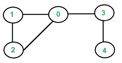
### Cycle in directed graph
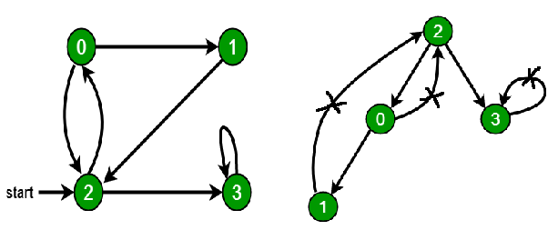
## References
General information:
- [Wikipedia](https://en.wikipedia.org/wiki/Cycle_(graph_theory))
Cycles in undirected graphs:
- [Detect Cycle in Undirected Graph on GeeksForGeeks](https://www.geeksforgeeks.org/detect-cycle-undirected-graph/)
- [Detect Cycle in Undirected Graph Algorithm on YouTube](https://www.youtube.com/watch?v=n_t0a_8H8VY&list=PLLXdhg_r2hKA7DPDsunoDZ-Z769jWn4R8)
Cycles in directed graphs:
- [Detect Cycle in Directed Graph on GeeksForGeeks](https://www.geeksforgeeks.org/detect-cycle-in-a-graph/)
- [Detect Cycle in Directed Graph Algorithm on YouTube](https://www.youtube.com/watch?v=rKQaZuoUR4M&list=PLLXdhg_r2hKA7DPDsunoDZ-Z769jWn4R8)
================================================
FILE: src/algorithms/graph/detect-cycle/__test__/detectDirectedCycle.test.js
================================================
import GraphVertex from '../../../../data-structures/graph/GraphVertex';
import GraphEdge from '../../../../data-structures/graph/GraphEdge';
import Graph from '../../../../data-structures/graph/Graph';
import detectDirectedCycle from '../detectDirectedCycle';
describe('detectDirectedCycle', () => {
it('should detect directed cycle', () => {
const vertexA = new GraphVertex('A');
const vertexB = new GraphVertex('B');
const vertexC = new GraphVertex('C');
const vertexD = new GraphVertex('D');
const vertexE = new GraphVertex('E');
const vertexF = new GraphVertex('F');
const edgeAB = new GraphEdge(vertexA, vertexB);
const edgeBC = new GraphEdge(vertexB, vertexC);
const edgeAC = new GraphEdge(vertexA, vertexC);
const edgeDA = new GraphEdge(vertexD, vertexA);
const edgeDE = new GraphEdge(vertexD, vertexE);
const edgeEF = new GraphEdge(vertexE, vertexF);
const edgeFD = new GraphEdge(vertexF, vertexD);
const graph = new Graph(true);
graph
.addEdge(edgeAB)
.addEdge(edgeBC)
.addEdge(edgeAC)
.addEdge(edgeDA)
.addEdge(edgeDE)
.addEdge(edgeEF);
expect(detectDirectedCycle(graph)).toBeNull();
graph.addEdge(edgeFD);
expect(detectDirectedCycle(graph)).toEqual({
D: vertexF,
F: vertexE,
E: vertexD,
});
});
});
================================================
FILE: src/algorithms/graph/detect-cycle/__test__/detectUndirectedCycle.test.js
================================================
import GraphVertex from '../../../../data-structures/graph/GraphVertex';
import GraphEdge from '../../../../data-structures/graph/GraphEdge';
import Graph from '../../../../data-structures/graph/Graph';
import detectUndirectedCycle from '../detectUndirectedCycle';
describe('detectUndirectedCycle', () => {
it('should detect undirected cycle', () => {
const vertexA = new GraphVertex('A');
const vertexB = new GraphVertex('B');
const vertexC = new GraphVertex('C');
const vertexD = new GraphVertex('D');
const vertexE = new GraphVertex('E');
const vertexF = new GraphVertex('F');
const edgeAF = new GraphEdge(vertexA, vertexF);
const edgeAB = new GraphEdge(vertexA, vertexB);
const edgeBE = new GraphEdge(vertexB, vertexE);
const edgeBC = new GraphEdge(vertexB, vertexC);
const edgeCD = new GraphEdge(vertexC, vertexD);
const edgeDE = new GraphEdge(vertexD, vertexE);
const graph = new Graph();
graph
.addEdge(edgeAF)
.addEdge(edgeAB)
.addEdge(edgeBE)
.addEdge(edgeBC)
.addEdge(edgeCD);
expect(detectUndirectedCycle(graph)).toBeNull();
graph.addEdge(edgeDE);
expect(detectUndirectedCycle(graph)).toEqual({
B: vertexC,
C: vertexD,
D: vertexE,
E: vertexB,
});
});
});
================================================
FILE: src/algorithms/graph/detect-cycle/__test__/detectUndirectedCycleUsingDisjointSet.test.js
================================================
import GraphVertex from '../../../../data-structures/graph/GraphVertex';
import GraphEdge from '../../../../data-structures/graph/GraphEdge';
import Graph from '../../../../data-structures/graph/Graph';
import detectUndirectedCycleUsingDisjointSet from '../detectUndirectedCycleUsingDisjointSet';
describe('detectUndirectedCycleUsingDisjointSet', () => {
it('should detect undirected cycle', () => {
const vertexA = new GraphVertex('A');
const vertexB = new GraphVertex('B');
const vertexC = new GraphVertex('C');
const vertexD = new GraphVertex('D');
const vertexE = new GraphVertex('E');
const vertexF = new GraphVertex('F');
const edgeAF = new GraphEdge(vertexA, vertexF);
const edgeAB = new GraphEdge(vertexA, vertexB);
const edgeBE = new GraphEdge(vertexB, vertexE);
const edgeBC = new GraphEdge(vertexB, vertexC);
const edgeCD = new GraphEdge(vertexC, vertexD);
const edgeDE = new GraphEdge(vertexD, vertexE);
const graph = new Graph();
graph
.addEdge(edgeAF)
.addEdge(edgeAB)
.addEdge(edgeBE)
.addEdge(edgeBC)
.addEdge(edgeCD);
expect(detectUndirectedCycleUsingDisjointSet(graph)).toBe(false);
graph.addEdge(edgeDE);
expect(detectUndirectedCycleUsingDisjointSet(graph)).toBe(true);
});
});
================================================
FILE: src/algorithms/graph/detect-cycle/detectDirectedCycle.js
================================================
import depthFirstSearch from '../depth-first-search/depthFirstSearch';
/**
* Detect cycle in directed graph using Depth First Search.
*
* @param {Graph} graph
*/
export default function detectDirectedCycle(graph) {
let cycle = null;
// Will store parents (previous vertices) for all visited nodes.
// This will be needed in order to specify what path exactly is a cycle.
const dfsParentMap = {};
// White set (UNVISITED) contains all the vertices that haven't been visited at all.
const whiteSet = {};
// Gray set (VISITING) contains all the vertices that are being visited right now
// (in current path).
const graySet = {};
// Black set (VISITED) contains all the vertices that has been fully visited.
// Meaning that all children of the vertex has been visited.
const blackSet = {};
// If we encounter vertex in gray set it means that we've found a cycle.
// Because when vertex in gray set it means that its neighbors or its neighbors
// neighbors are still being explored.
// Init white set and add all vertices to it.
/** @param {GraphVertex} vertex */
graph.getAllVertices().forEach((vertex) => {
whiteSet[vertex.getKey()] = vertex;
});
// Describe BFS callbacks.
const callbacks = {
enterVertex: ({ currentVertex, previousVertex }) => {
if (graySet[currentVertex.getKey()]) {
// If current vertex already in grey set it means that cycle is detected.
// Let's detect cycle path.
cycle = {};
let currentCycleVertex = currentVertex;
let previousCycleVertex = previousVertex;
while (previousCycleVertex.getKey() !== currentVertex.getKey()) {
cycle[currentCycleVertex.getKey()] = previousCycleVertex;
currentCycleVertex = previousCycleVertex;
previousCycleVertex = dfsParentMap[previousCycleVertex.getKey()];
}
cycle[currentCycleVertex.getKey()] = previousCycleVertex;
} else {
// Otherwise let's add current vertex to gray set and remove it from white set.
graySet[currentVertex.getKey()] = currentVertex;
delete whiteSet[currentVertex.getKey()];
// Update DFS parents list.
dfsParentMap[currentVertex.getKey()] = previousVertex;
}
},
leaveVertex: ({ currentVertex }) => {
// If all node's children has been visited let's remove it from gray set
// and move it to the black set meaning that all its neighbors are visited.
blackSet[currentVertex.getKey()] = currentVertex;
delete graySet[currentVertex.getKey()];
},
allowTraversal: ({ nextVertex }) => {
// If cycle was detected we must forbid all further traversing since it will
// cause infinite traversal loop.
if (cycle) {
return false;
}
// Allow traversal only for the vertices that are not in black set
// since all black set vertices have been already visited.
return !blackSet[nextVertex.getKey()];
},
};
// Start exploring vertices.
while (Object.keys(whiteSet).length) {
// Pick fist vertex to start BFS from.
const firstWhiteKey = Object.keys(whiteSet)[0];
const startVertex = whiteSet[firstWhiteKey];
// Do Depth First Search.
depthFirstSearch(graph, startVertex, callbacks);
}
return cycle;
}
================================================
FILE: src/algorithms/graph/detect-cycle/detectUndirectedCycle.js
================================================
import depthFirstSearch from '../depth-first-search/depthFirstSearch';
/**
* Detect cycle in undirected graph using Depth First Search.
*
* @param {Graph} graph
*/
export default function detectUndirectedCycle(graph) {
let cycle = null;
// List of vertices that we have visited.
const visitedVertices = {};
// List of parents vertices for every visited vertex.
const parents = {};
// Callbacks for DFS traversing.
const callbacks = {
allowTraversal: ({ currentVertex, nextVertex }) => {
// Don't allow further traversal in case if cycle has been detected.
if (cycle) {
return false;
}
// Don't allow traversal from child back to its parent.
const currentVertexParent = parents[currentVertex.getKey()];
const currentVertexParentKey = currentVertexParent ? currentVertexParent.getKey() : null;
return currentVertexParentKey !== nextVertex.getKey();
},
enterVertex: ({ currentVertex, previousVertex }) => {
if (visitedVertices[currentVertex.getKey()]) {
// Compile cycle path based on parents of previous vertices.
cycle = {};
let currentCycleVertex = currentVertex;
let previousCycleVertex = previousVertex;
while (previousCycleVertex.getKey() !== currentVertex.getKey()) {
cycle[currentCycleVertex.getKey()] = previousCycleVertex;
currentCycleVertex = previousCycleVertex;
previousCycleVertex = parents[previousCycleVertex.getKey()];
}
cycle[currentCycleVertex.getKey()] = previousCycleVertex;
} else {
// Add next vertex to visited set.
visitedVertices[currentVertex.getKey()] = currentVertex;
parents[currentVertex.getKey()] = previousVertex;
}
},
};
// Start DFS traversing.
const startVertex = graph.getAllVertices()[0];
depthFirstSearch(graph, startVertex, callbacks);
return cycle;
}
================================================
FILE: src/algorithms/graph/detect-cycle/detectUndirectedCycleUsingDisjointSet.js
================================================
import DisjointSet from '../../../data-structures/disjoint-set/DisjointSet';
/**
* Detect cycle in undirected graph using disjoint sets.
*
* @param {Graph} graph
*/
export default function detectUndirectedCycleUsingDisjointSet(graph) {
// Create initial singleton disjoint sets for each graph vertex.
/** @param {GraphVertex} graphVertex */
const keyExtractor = (graphVertex) => graphVertex.getKey();
const disjointSet = new DisjointSet(keyExtractor);
graph.getAllVertices().forEach((graphVertex) => disjointSet.makeSet(graphVertex));
// Go trough all graph edges one by one and check if edge vertices are from the
// different sets. In this case joint those sets together. Do this until you find
// an edge where to edge vertices are already in one set. This means that current
// edge will create a cycle.
let cycleFound = false;
/** @param {GraphEdge} graphEdge */
graph.getAllEdges().forEach((graphEdge) => {
if (disjointSet.inSameSet(graphEdge.startVertex, graphEdge.endVertex)) {
// Cycle found.
cycleFound = true;
} else {
disjointSet.union(graphEdge.startVertex, graphEdge.endVertex);
}
});
return cycleFound;
}
================================================
FILE: src/algorithms/graph/dijkstra/README.de-DE.md
================================================
# Dijkstra-Algorithmus
_Lies dies in anderen Sprachen:_
[_English_](README.md),
[_한국어_](README.ko-KR.md),
[_日本語_](README.ja-JP.md),
[_简体中文_](README.zh-CN.md),
[_繁體中文_](README.zh-TW.md),
[_Українська_](README.uk-UA.md),
[_Español_](README.es-ES.md),
[_Français_](README.fr-FR.md),
[_Deutsch_](README.de-DE.md),
[_עברית_](README.he-IL.md)
Der Dijkstra-Algorithmus ist ein Algorithmus zur Bestimmung der kürzesten Wege zwischen Knoten in einem Graphen, der beispielsweise Straßennetze darstellen kann.
Der Algorithmus existiert in vielen Varianten; die ursprüngliche Version von Dijkstra fand den kürzesten Weg zwischen zwei Knoten, aber eine gebräuchlichere Variante fixiert einen einzelnen Knoten als „Quellknoten“ und findet die kürzesten Wege von dieser Quelle zu allen anderen Knoten im Graphen. Das Ergebnis ist ein sogenannter „kürzester-Wege-Baum“ (Shortest-Path Tree).

Der Dijkstra-Algorithmus findet den kürzesten Weg zwischen `a` und `b`.
Er wählt den unbesuchten Knoten mit der kleinsten aktuellen Entfernung,
berechnet die Distanzen zu jedem unbesuchten Nachbarn über diesen Knoten
und aktualisiert die Entfernung des Nachbarn, wenn sie kleiner ist.
Nachdem alle Nachbarn überprüft wurden, wird der Knoten als besucht markiert (rot dargestellt).
## Praktische Anwendungen des Dijkstra-Algorithmus
- GPS- und Navigationssysteme
- Optimierung von Routen im öffentlichen Verkehr und im Flugverkehr
- Internet-Routing (OSPF-, IS-IS-Protokolle)
- Optimierung von Netzwerkverkehr und Latenzzeiten
- Pfadsuche in Computerspielen (kürzester Weg auf Karten)
- Routenoptimierung in Logistik und Lieferketten
- Planung von Transport- und Versorgungsnetzen
## Schritt-für-Schritt-Beispiel des Dijkstra-Algorithmus
Nehmen wir an, wir haben einen gewichteten Graphen, bei dem jede Kante eine Distanz zwischen Knoten hat.
Zum Beispiel beträgt die Entfernung zwischen Knoten `A` und `B` `7 Meter` (oder kurz `7m`).
Der Algorithmus verwendet eine [Prioritätswarteschlange](../../../data-structures/priority-queue/),
um immer den nächsten unbesuchten Knoten mit der kleinsten Entfernung vom Startknoten zu entnehmen.
Der Startknoten hat per Definition eine Entfernung von `0m` zu sich selbst.
Wir beginnen also mit diesem Knoten – er ist der einzige in der Prioritätswarteschlange zu Beginn.
Die restlichen Knoten werden während der Graphdurchquerung (beim Besuchen der Nachbarn) später hinzugefügt.

Jeder Nachbar des aus der Warteschlange entnommenen Knotens wird überprüft, um die Entfernung vom Startpunkt zu berechnen.
Zum Beispiel: Die Entfernung von `A` nach `B` beträgt `0m + 7m = 7m`.
Jedes Mal, wenn wir einen neuen, noch nicht gesehenen Nachbarn besuchen, fügen wir ihn der Prioritätswarteschlange hinzu, wobei die Priorität die Distanz zum Startknoten ist.
Der Knoten `B` wird mit der Priorität 7m in die Warteschlange eingefügt, um später besucht zu werden.

Als Nächstes besuchen wir den Nachbarn `C` von `A`.
Die Entfernung vom Startknoten `A` zu `C` beträgt `0m + 9m = 9m`.
Der Knoten `C` wird ebenfalls in die Prioritätswarteschlange eingefügt.

Dasselbe gilt für den Knoten `F`.
Die aktuelle Entfernung von `A` zu `F` ist `0m + 14m = 14m`.
`F` wird in die Warteschlange eingefügt, um später besucht zu werden.

Nachdem alle Nachbarn des aktuellen Knotens überprüft wurden, wird dieser Knoten zur `visited`-Menge hinzugefügt.
Solche Knoten werden in den nächsten Schritten nicht erneut besucht.
Nun entnehmen wir aus der Prioritätswarteschlange den nächsten Knoten mit der kürzesten Distanz zur Quelle und beginnen, seine Nachbarn zu besuchen.

Wenn der Knoten, den wir besuchen (in diesem Fall `C`), bereits in der Warteschlange ist,
bedeutet das, dass die Distanz zu ihm bereits von einem anderen Pfad (`A → C`) berechnet wurde.
Wenn die aktuelle Distanz (über `A → B → C`) kürzer ist, aktualisieren wir den Wert in der Warteschlange.
Ist sie länger, bleibt sie unverändert.
Beim Besuch von `C` über `B` (`A → B → C`) beträgt die Distanz `7m + 10m = 17m`.
Dies ist länger als die bereits gespeicherte Distanz `9m` für `A → C`.
Daher ignorieren wir diesen längeren Pfad.

Wir besuchen einen weiteren Nachbarn von `B`, nämlich `D`.
Die Entfernung zu `D` beträgt `7m + 15m = 22m`.
Da `D` noch nicht besucht wurde und nicht in der Warteschlange ist, fügen wir ihn mit der Priorität `22m` hinzu.

An diesem Punkt wurden alle Nachbarn von `B` besucht, daher wird `B` zur `visited`-Menge hinzugefügt.
Als Nächstes entnehmen wir aus der Warteschlange den Knoten, der dem Ursprung am nächsten ist.

Wir besuchen die unbesuchten Nachbarn von `C`.
Die Distanz zu `F` über `C` (`A → C → F`) beträgt `9m + 2m = 11m`.
Dies ist kürzer als der bisher gespeicherte Weg `A → F` von `14m`.
In diesem Fall aktualisieren wir die Distanz zu `F` auf `11m` und passen ihre Priorität in der Warteschlange an.
Wir haben einen kürzeren Weg zu `F` gefunden.

Dasselbe gilt für `D`.
Wir haben einen kürzeren Pfad zu `D` gefunden – der Weg `A → C → D` ist kürzer als `A → B → D`.
Die Distanz wird von `22m` auf `20m` aktualisiert.

Alle Nachbarn von `C` wurden besucht, daher fügen wir `C` zur `visited`-Menge hinzu.
Wir entnehmen den nächsten Knoten aus der Warteschlange, der `F` ist.

Wir notieren die Distanz zu `E` als `11m + 9m = 20m`.

Wir fügen `F` zur `visited`-Menge hinzu und entnehmen den nächsten Knoten `D`.

Die Distanz zu `E` über `D` ist `20m + 6m = 26m`.
Das ist länger als die bereits berechnete Distanz von `20m` über `F`.
Daher verwerfen wir diesen längeren Weg.

Der Knoten `D` ist jetzt besucht.

Auch der Knoten `E` wurde besucht.
Die Durchquerung des Graphen ist abgeschlossen.

Nun kennen wir die kürzesten Distanzen von jedem Knoten ausgehend vom Startknoten `A`.
In der Praxis speichert man während der Berechnungen zusätzlich die `previousVertices` (vorherige Knoten),
um die genaue Reihenfolge der Knoten im kürzesten Pfad rekonstruieren zu können.
Zum Beispiel ist der kürzeste Pfad von `A` nach `E`: `A → C → F → E`.
## Beispielimplementierung
- [dijkstra.js](./dijkstra.js)
## Quellen
- [Wikipedia](https://de.wikipedia.org/wiki/Dijkstra-Algorithmus)
- [YouTube – Nathaniel Fan](https://www.youtube.com/watch?v=gdmfOwyQlcI&list=PLLXdhg_r2hKA7DPDsunoDZ-Z769jWn4R8)
- [YouTube – Tushar Roy](https://www.youtube.com/watch?v=lAXZGERcDf4&list=PLLXdhg_r2hKA7DPDsunoDZ-Z769jWn4R8)
================================================
FILE: src/algorithms/graph/dijkstra/README.es-ES.md
================================================
# Algoritmo de Dijkstra
_Lee esto en otros idiomas:_
[_English_](README.md),
[_한국어_](README.ko-KR.md),
[_日本語_](README.ja-JP.md),
[_简体中文_](README.zh-CN.md),
[_繁體中文_](README.zh-TW.md),
[_Українська_](README.uk-UA.md),
[_Español_](README.es-ES.md),
[_Français_](README.fr-FR.md),
[_Deutsch_](README.de-DE.md),
[_עברית_](README.he-IL.md)
El algoritmo de Dijkstra es un algoritmo para encontrar los caminos más cortos entre nodos en un grafo, que puede representar, por ejemplo, redes de carreteras.
El algoritmo existe en muchas variantes; la versión original de Dijkstra encontraba el camino más corto entre dos nodos, pero una variante más común fija un solo nodo como el "nodo fuente" y encuentra los caminos más cortos desde la fuente hacia todos los demás nodos del grafo, produciendo un árbol de caminos más cortos.

El algoritmo de Dijkstra busca el camino más corto entre `a` y `b`.
Selecciona el vértice no visitado con la menor distancia, calcula la distancia a través de él hacia cada vecino no visitado, y actualiza la distancia del vecino si es menor. Marca el vértice como visitado (en rojo) cuando se han procesado todos sus vecinos.
## Aplicaciones prácticas del algoritmo de Dijkstra
- Sistemas GPS / navegación
- Optimización de rutas de transporte público y aerolíneas
- Enrutamiento de Internet (protocolos OSPF, IS-IS)
- Optimización del tráfico y la latencia en redes
- Búsqueda de caminos en videojuegos (camino más corto en mapas)
- Optimización de rutas de logística y entrega
- Diseño de redes de transporte y cadenas de suministro
## Ejemplo paso a paso del algoritmo de Dijkstra
Supongamos que tenemos un grafo ponderado de nodos, donde cada arista tiene un valor de distancia entre los nodos. Por ejemplo, la distancia entre el nodo `A` y el nodo `B` es de `7 metros` (o simplemente `7m` para abreviar).
El algoritmo utiliza una [cola de prioridad](../../../data-structures/priority-queue/) para obtener siempre el siguiente vértice no visitado con la menor distancia desde el nodo de origen.
El nodo inicial, por definición, tiene una distancia de `0m` desde sí mismo. Así que comenzamos con él — el único nodo en la cola de prioridad al inicio.
El resto de los nodos se agregará a la cola de prioridad más tarde, durante la exploración del grafo (al visitar los vecinos).

Cada vecino del nodo extraído de la cola se recorre para calcular la distancia desde el origen.
Por ejemplo, la distancia de `A` a `B` es `0m + 7m = 7m`.
Cada vez que visitamos un vecino aún no visto, lo agregamos a la cola de prioridad, donde la prioridad es la distancia al nodo vecino desde el origen.
El nodo `B` se agrega a la cola de prioridad mínima para ser recorrido más adelante.

Visitamos el siguiente vecino `C` del nodo `A`.
La distancia desde el nodo de origen `A` hasta `C` es `0m + 9m = 9m`.
El nodo `C` se agrega a la cola de prioridad mínima para recorrerlo más tarde.

Lo mismo ocurre con el nodo `F`.
La distancia actual de `A` a `F` es `0m + 14m = 14m`.
El nodo `F` se agrega a la cola de prioridad mínima para ser recorrido más adelante.

Una vez que se han revisado todos los vecinos del nodo actual, este se agrega al conjunto `visited`. No queremos volver a visitar estos nodos más adelante.
Ahora extraemos de la cola el siguiente nodo más cercano al origen (el de menor distancia) y comenzamos a visitar sus vecinos.

Si el nodo que estamos visitando (en este caso, `C`) ya está en la cola, significa que ya habíamos calculado la distancia hacia él, pero desde otro camino (`A → C`).
Si la distancia actual (desde el camino `A → B → C`) es menor que la calculada antes, actualizamos la distancia (en la cola de prioridad) con la más corta, ya que buscamos los caminos más cortos.
Si la distancia es mayor, la dejamos como está.
Al visitar el nodo `C` a través de `B` (camino `A → B → C`), vemos que la distancia sería `7m + 10m = 17m`.
Esto es más largo que la distancia ya registrada de `9m` para el camino `A → C`. En estos casos, simplemente ignoramos la distancia más larga.

Visitamos otro vecino de `B`, que es `D`.
La distancia hacia `D` es `7m + 15m = 22m`.
Como aún no hemos visitado `D` y no está en la cola de prioridad, la agregamos con una prioridad (distancia) de `22m`.

En este punto, todos los vecinos de `B` han sido recorridos, así que agregamos `B` al conjunto `visited`.
Luego extraemos el nodo más cercano al origen desde la cola de prioridad.

Recorremos los vecinos no visitados del nodo `C`.
La distancia hacia `F` a través de `C` (camino `A → C → F`) es `9m + 2m = 11m`.
Esto es más corto que el camino anterior `A → F` de `14m`.
En este caso, actualizamos la distancia de `F` a `11m` y su prioridad en la cola. Hemos encontrado un camino más corto hacia `F`.

Lo mismo ocurre con `D`.
Hemos encontrado un camino más corto hacia `D`, donde `A → C → D` es más corto que `A → B → D`.
Actualizamos la distancia de `22m` a `20m`.

Todos los vecinos de `C` han sido recorridos, así que podemos agregar `C` al conjunto `visited`.
Extraemos de la cola el siguiente nodo más cercano, que es `F`.

Registramos la distancia hacia `E` como `11m + 9m = 20m`.

Agregamos el nodo `F` al conjunto `visited` y extraemos el siguiente nodo más cercano, `D`.

La distancia hacia `E` a través de `D` es `20m + 6m = 26m`.
Esto es más largo que la distancia ya calculada hacia `E` desde `F`, que es `20m`.
Podemos descartar la distancia más larga.

El nodo `D` ahora está visitado.

El nodo `E` también ha sido visitado.
Hemos terminado de recorrer el grafo.

Ahora conocemos las distancias más cortas desde el nodo inicial `A` hacia cada nodo.
En la práctica, durante el cálculo de distancias también registramos los `previousVertices` (vértices anteriores) para poder mostrar la secuencia exacta de nodos que forman el camino más corto.
Por ejemplo, el camino más corto de `A` a `E` es `A → C → F → E`.
## Ejemplo de implementación
- [dijkstra.js](./dijkstra.js)
## Referencias
- [Wikipedia](https://es.wikipedia.org/wiki/Algoritmo_de_Dijkstra)
- [YouTube - Nathaniel Fan](https://www.youtube.com/watch?v=gdmfOwyQlcI&list=PLLXdhg_r2hKA7DPDsunoDZ-Z769jWn4R8)
- [YouTube - Tushar Roy](https://www.youtube.com/watch?v=lAXZGERcDf4&list=PLLXdhg_r2hKA7DPDsunoDZ-Z769jWn4R8)
================================================
FILE: src/algorithms/graph/dijkstra/README.fr-FR.md
================================================
# Algorithme de Dijkstra
_Lire ceci dans d’autres langues :_
[_English_](README.md),
[_한국어_](README.ko-KR.md),
[_日本語_](README.ja-JP.md),
[_简体中文_](README.zh-CN.md),
[_繁體中文_](README.zh-TW.md),
[_Українська_](README.uk-UA.md),
[_Español_](README.es-ES.md),
[_Français_](README.fr-FR.md),
[_Deutsch_](README.de-DE.md),
[_עברית_](README.he-IL.md)
L’algorithme de Dijkstra est un algorithme permettant de trouver les plus courts chemins entre des nœuds dans un graphe, pouvant représenter, par exemple, un réseau routier.
Il existe plusieurs variantes de cet algorithme. La version originale de Dijkstra trouvait le plus court chemin entre deux nœuds, mais la version la plus courante fixe un seul nœud comme « nœud source » et calcule les plus courts chemins de cette source vers tous les autres nœuds du graphe, produisant ainsi un arbre des plus courts chemins.

L’algorithme de Dijkstra trouve le plus court chemin entre `a` et `b`.
Il sélectionne le sommet non visité avec la plus petite distance, calcule la distance à travers ce sommet vers chacun de ses voisins non visités, et met à jour la distance du voisin si celle-ci est plus courte.
Le sommet est ensuite marqué comme visité (en rouge) lorsque tous ses voisins ont été traités.
## Applications pratiques de l’algorithme de Dijkstra
- Systèmes GPS / navigation
- Optimisation des itinéraires de transport public et d’avions
- Routage Internet (protocoles OSPF, IS-IS)
- Optimisation du trafic et de la latence réseau
- Recherche de chemin dans les jeux vidéo (chemin le plus court sur une carte)
- Optimisation des itinéraires de livraison et de logistique
- Conception de réseaux de transport et de chaînes d’approvisionnement
## Exemple pas à pas de l’algorithme de Dijkstra
Supposons que nous ayons un graphe pondéré de nœuds, où chaque arête possède une distance entre deux nœuds.
Par exemple, la distance entre le nœud `A` et le nœud `B` est de `7 mètres` (ou simplement `7m`).
L’algorithme utilise une [file de priorité](../../../data-structures/priority-queue/) pour toujours extraire le prochain sommet non visité ayant la plus petite distance depuis le nœud d’origine.
Le nœud de départ, par définition, a une distance de `0m` depuis lui-même.
Nous commençons donc avec ce nœud, le seul présent dans la file de priorité au départ.
Les autres nœuds seront ajoutés à la file de priorité plus tard, pendant la traversée du graphe (en visitant les voisins).

Chaque voisin du nœud extrait de la file est parcouru afin de calculer la distance à partir du nœud d’origine.
Par exemple, la distance de `A` à `B` est `0m + 7m = 7m`.
Chaque fois qu’un voisin encore non visité est découvert, il est ajouté à la file de priorité, la priorité correspondant à la distance depuis le nœud d’origine.
Le nœud `B` est ajouté à la file de priorité minimale pour être traité plus tard.

Nous visitons le voisin suivant, `C`, du nœud `A`.
La distance depuis le nœud d’origine `A` vers `C` est `0m + 9m = 9m`.
Le nœud `C` est ajouté à la file de priorité minimale pour être parcouru ultérieurement.

Même chose pour le nœud `F`.
La distance actuelle de `A` à `F` est `0m + 14m = 14m`.
Le nœud `F` est ajouté à la file de priorité minimale pour être visité plus tard.

Une fois que tous les voisins du nœud actuel ont été examinés, ce nœud est ajouté à l’ensemble `visited`.
Nous ne souhaitons plus revisiter ces nœuds lors des prochaines itérations.
Nous extrayons maintenant de la file le nœud le plus proche de la source (celui ayant la plus courte distance) et commençons à visiter ses voisins.

Si le nœud que nous visitons (dans ce cas, `C`) est déjà présent dans la file, cela signifie que sa distance a déjà été calculée via un autre chemin (`A → C`).
Si la nouvelle distance (depuis le chemin `A → B → C`) est plus courte, nous mettons à jour la distance dans la file de priorité.
Si elle est plus longue, nous la laissons telle quelle.
En visitant le nœud `C` via `B` (chemin `A → B → C`), nous trouvons que la distance est `7m + 10m = 17m`.
Ceci est plus long que la distance enregistrée de `9m` pour le chemin `A → C`.
Dans ce cas, nous ignorons simplement cette distance plus longue.

Nous visitons un autre voisin de `B`, à savoir `D`.
La distance vers `D` est `7m + 15m = 22m`.
Comme `D` n’a pas encore été visité et n’est pas dans la file, nous l’ajoutons avec une priorité (distance) de `22m`.

À ce stade, tous les voisins de `B` ont été parcourus, donc nous ajoutons `B` à l’ensemble `visited`.
Ensuite, nous extrayons de la file le nœud le plus proche du nœud d’origine.

Nous parcourons les voisins non visités du nœud `C`.
La distance vers `F` via `C` (chemin `A → C → F`) est `9m + 2m = 11m`.
C’est plus court que la distance précédemment enregistrée de `14m` pour le chemin `A → F`.
Nous mettons donc à jour la distance de `F` à `11m` et ajustons sa priorité dans la file.
Nous venons de trouver un chemin plus court vers `F`.

Même chose pour `D`.
Nous avons trouvé un chemin plus court vers `D` : `A → C → D` est plus court que `A → B → D`.
Nous mettons à jour la distance de `22m` à `20m`.

Tous les voisins de `C` ont été parcourus, donc nous pouvons ajouter `C` à l’ensemble `visited`.
Nous extrayons maintenant de la file le prochain nœud le plus proche, `F`.

Nous enregistrons la distance vers `E` comme `11m + 9m = 20m`.

Nous ajoutons `F` à l’ensemble `visited` et extrayons ensuite `D`, le prochain nœud le plus proche.

La distance vers `E` via `D` est `20m + 6m = 26m`.
C’est plus long que la distance déjà calculée depuis `F` (`20m`).
Nous pouvons donc ignorer cette distance plus longue.

Le nœud `D` est maintenant visité.

Le nœud `E` est maintenant visité également.
La traversée du graphe est terminée.

Nous connaissons maintenant les distances les plus courtes vers chaque nœud depuis le nœud de départ `A`.
En pratique, pendant le calcul des distances, on enregistre également les `previousVertices` (nœuds précédents) pour pouvoir reconstruire la séquence exacte des nœuds qui forment le chemin le plus court.
Par exemple, le chemin le plus court de `A` à `E` est `A → C → F → E`.
## Exemple d’implémentation
- [dijkstra.js](./dijkstra.js)
## Références
- [Wikipédia](https://fr.wikipedia.org/wiki/Algorithme_de_Dijkstra)
- [YouTube - Nathaniel Fan](https://www.youtube.com/watch?v=gdmfOwyQlcI&list=PLLXdhg_r2hKA7DPDsunoDZ-Z769jWn4R8)
- [YouTube - Tushar Roy](https://www.youtube.com/watch?v=lAXZGERcDf4&list=PLLXdhg_r2hKA7DPDsunoDZ-Z769jWn4R8)
================================================
FILE: src/algorithms/graph/dijkstra/README.he-IL.md
================================================
# אלגוריתם דייקסטרה (Dijkstra's Algorithm)
_קרא בשפות אחרות:_
[_English_](README.md),
[_한국어_](README.ko-KR.md),
[_日本語_](README.ja-JP.md),
[_简体中文_](README.zh-CN.md),
[_繁體中文_](README.zh-TW.md),
[_Українська_](README.uk-UA.md),
[_Español_](README.es-ES.md),
[_Français_](README.fr-FR.md),
[_Deutsch_](README.de-DE.md),
[_עברית_](README.he-IL.md)
אלגוריתם דייקסטרה הוא אלגוריתם למציאת המסלולים הקצרים ביותר בין צמתים בגרף, שיכול לייצג למשל רשת כבישים.
לאלגוריתם יש מספר גרסאות; הגרסה המקורית של דייקסטרה מצאה את המסלול הקצר ביותר בין שני צמתים, אך גרסה נפוצה יותר קובעת צומת אחד כ"צומת מקור" ומוצאת את המסלולים הקצרים ביותר ממנו לכל שאר הצמתים בגרף, וכך נוצרת עץ מסלולים קצרים (Shortest-Path Tree).

אלגוריתם דייקסטרה למציאת המסלול הקצר ביותר בין `a` ל־`b`.
הוא בוחר את הצומת שלא ביקרו בו שעד כה יש לו את המרחק הקטן ביותר,
מחשב את המרחק דרכו לכל שכן שלא ביקרו בו,
ומעדכן את המרחק אם נמצא מסלול קצר יותר.
כאשר מסיימים לבדוק את כל השכנים, מסמנים את הצומת כ"ביקור הושלם" (אדום).
## שימושים מעשיים של אלגוריתם דייקסטרה
- מערכות GPS / ניווט
- אופטימיזציה של מסלולי תחבורה ציבורית וטיסות
- ניתוב באינטרנט (פרוטוקולים OSPF, IS-IS)
- אופטימיזציה של תעבורת רשת וזמני השהיה
- חיפוש מסלולים במשחקים (המסלול הקצר ביותר במפה)
- אופטימיזציה של מסלולי משלוחים ולוגיסטיקה
- תכנון רשתות תחבורה ושרשראות אספקה
## דוגמה שלב-אחר-שלב לאלגוריתם דייקסטרה
נניח שיש לנו גרף משוקלל של צמתים, שבו לכל קשת יש ערך מרחק בין צמתים.
לדוגמה, המרחק בין הצומת `A` לצומת `B` הוא `7 מטרים` (או בקיצור `7m`).
האלגוריתם משתמש ב[תור עדיפויות](../../../data-structures/priority-queue/) כדי תמיד לבחור את הצומת שלא ביקרו בו עם המרחק הקטן ביותר מהצומת ההתחלתי.
צומת ההתחלה, על פי ההגדרה, נמצא במרחק `0m` מעצמו.
לכן מתחילים ממנו — הצומת היחיד בתור העדיפויות בתחילת התהליך.
שאר הצמתים יתווספו לתור במהלך המעבר בגרף (בעת ביקור בשכנים).

כל שכן של הצומת שנשלף מהתור נבדק כדי לחשב את המרחק אליו מהמקור.
לדוגמה, המרחק מ־`A` ל־`B` הוא `0m + 7m = 7m`.
בכל פעם שמבקרים שכן חדש שטרם נבדק, מוסיפים אותו לתור העדיפויות,
כאשר העדיפות נקבעת לפי המרחק מהמקור.
הצומת `B` נוסף לתור העדיפויות המינימלי כדי לעבור עליו מאוחר יותר.

מבקרים את השכן הבא של `A`, שהוא `C`.
המרחק מ־`A` ל־`C` הוא `0m + 9m = 9m`.
הצומת `C` נוסף גם הוא לתור העדיפויות.

כנ"ל לגבי הצומת `F`.
המרחק הנוכחי מ־`A` ל־`F` הוא `0m + 14m = 14m`.
`F` נוסף לתור כדי לעבור עליו בהמשך.

לאחר שכל השכנים של הצומת הנוכחי נבדקו, מוסיפים אותו לקבוצת `visited`.
אין צורך לבקר בו שוב.
כעת נשלוף מהתור את הצומת הקרוב ביותר למקור (בעל המרחק הקצר ביותר)
ונתחיל לבקר את שכניו.

אם הצומת שבו אנו מבקרים (למשל `C`) כבר נמצא בתור,
המשמעות היא שכבר חישבנו את המרחק אליו, אבל ממסלול אחר (`A → C`).
אם המרחק הנוכחי (דרך המסלול `A → B → C`) קצר יותר, נעדכן אותו;
אם ארוך יותר — נשאיר אותו כפי שהוא.
לדוגמה, בעת ביקור ב־`C` דרך `B` (`A → B → C`), המרחק הוא `7m + 10m = 17m`.
זה ארוך יותר מהמרחק שכבר נרשם (`9m`), ולכן אין עדכון.

מבקרים שכן נוסף של `B`, שהוא `D`.
המרחק ל־`D` הוא `7m + 15m = 22m`.
מכיוון שטרם ביקרנו ב־`D` והוא אינו בתור, נוסיף אותו עם עדיפות (מרחק) של `22m`.

בשלב זה כל שכניו של `B` נבדקו, ולכן נוסיף את `B` לקבוצת `visited`.
לאחר מכן נשלוף את הצומת הקרוב ביותר למקור מהתור.

מבקרים את השכנים הלא-מבוקרים של `C`.
המרחק ל־`F` דרך `C` (המסלול `A → C → F`) הוא `9m + 2m = 11m`.
זה קצר יותר מהמרחק שנרשם קודם (`14m` ל־`A → F`).
לכן נעדכן את המרחק של `F` ל־`11m` ואת העדיפות שלו בתור.
מצאנו מסלול קצר יותר ל־`F`.

אותו הדבר עבור `D`.
מצאנו מסלול קצר יותר — `A → C → D` קצר מ־`A → B → D`.
נעדכן את המרחק מ־`22m` ל־`20m`.

כל שכניו של `C` נבדקו, ולכן נוסיף את `C` ל־`visited`.
נשלוף מהתור את הצומת הקרוב ביותר הבא — `F`.

נרשום את המרחק ל־`E` כ־`11m + 9m = 20m`.

נוסיף את `F` לקבוצת `visited`, ונשלוף את הצומת הקרוב הבא — `D`.

המרחק ל־`E` דרך `D` הוא `20m + 6m = 26m`.
זה ארוך יותר מהמרחק שכבר חושב (`20m` דרך `F`), ולכן נתעלם ממנו.

הצומת `D` כעת סומן כ"ביקור הושלם".

הצומת `E` גם סומן כ"ביקור הושלם".
סיימנו את המעבר בגרף.

כעת אנו יודעים את המרחקים הקצרים ביותר מכל צומת לנקודת ההתחלה `A`.
בפועל, במהלך חישוב המרחקים שומרים גם את ה־`previousVertices` (הצמתים הקודמים)
כדי שנוכל לשחזר את הרצף המדויק של הצמתים שמרכיבים את המסלול הקצר ביותר.
לדוגמה, המסלול הקצר מ־`A` ל־`E` הוא `A → C → F → E`.
## דוגמת מימוש
- [dijkstra.js](./dijkstra.js)
## מקורות
- [ויקיפדיה](https://he.wikipedia.org/wiki/אלגוריתם_דייקסטרה)
- [YouTube – Nathaniel Fan](https://www.youtube.com/watch?v=gdmfOwyQlcI&list=PLLXdhg_r2hKA7DPDsunoDZ-Z769jWn4R8)
- [YouTube – Tushar Roy](https://www.youtube.com/watch?v=lAXZGERcDf4&list=PLLXdhg_r2hKA7DPDsunoDZ-Z769jWn4R8)
================================================
FILE: src/algorithms/graph/dijkstra/README.ja-JP.md
================================================
# ダイクストラ法 (Dijkstra's Algorithm)
_他の言語で読む:_
[_English_](README.md),
[_한국어_](README.ko-KR.md),
[_日本語_](README.ja-JP.md),
[_简体中文_](README.zh-CN.md),
[_繁體中文_](README.zh-TW.md),
[_Українська_](README.uk-UA.md),
[_Español_](README.es-ES.md),
[_Français_](README.fr-FR.md),
[_Deutsch_](README.de-DE.md),
[_עברית_](README.he-IL.md)
ダイクストラ法は、グラフ内のノード間の最短経路を見つけるためのアルゴリズムです。
例えば道路網などを表すことができます。
このアルゴリズムにはいくつかのバリエーションがあります。
ダイクストラの元々の手法は、2つのノード間の最短経路を求めるものでしたが、
より一般的なバージョンでは、1つのノードを「始点(ソース)」として固定し、
その始点から他のすべてのノードまでの最短経路を求め、最短経路木(shortest-path tree)を生成します。

`a` から `b` への最短経路を見つけるダイクストラ法。
訪問していないノードの中で最も距離の短いノードを選び、
そのノードを経由して未訪問の隣接ノードへの距離を計算し、
もし短ければその距離を更新します。
すべての隣接ノードを処理したら、そのノードを訪問済み(赤色)としてマークします。
## ダイクストラ法の実用例
- GPS / ナビゲーションシステム
- 公共交通機関や航空路線の最適化
- インターネットルーティング(OSPF、IS-IS プロトコル)
- ネットワークトラフィックとレイテンシーの最適化
- ゲームにおける経路探索(マップ上の最短経路)
- 物流および配送ルートの最適化
- サプライチェーンや交通ネットワーク設計
## ダイクストラ法のステップごとの例
重み付きグラフがあり、各辺にはノード間の距離が設定されています。
たとえば、ノード `A` とノード `B` の距離が `7m` であるとします。
このアルゴリズムは、[優先度付きキュー](../../../data-structures/priority-queue/)を使用し、
常に始点から最も近い未訪問ノードを取り出します。
始点ノードは自分自身からの距離が `0m` なので、
最初にキューに入っているのはこのノードだけです。
他のノードは、グラフ探索中(隣接ノードを訪問する際)に後でキューに追加されます。

キューから取り出したノードの各隣接ノードについて、始点からの距離を計算します。
たとえば、`A` から `B` までの距離は `0m + 7m = 7m` です。
初めて訪れる隣接ノードは、始点からの距離を優先度としてキューに追加されます。
ノード `B` は、後で探索するために最小優先度キューに追加されます。

次に、ノード `A` のもう一つの隣接ノード `C` を訪問します。
始点 `A` から `C` までの距離は `0m + 9m = 9m` です。
ノード `C` も最小優先度キューに追加されます。

同様に、ノード `F` の場合、始点 `A` からの距離は `0m + 14m = 14m` です。
ノード `F` も後で探索するためにキューに追加します。

現在のノードのすべての隣接ノードを確認した後、
そのノードを `visited` セットに追加します。
このノードは今後再訪しません。
次に、始点から最も近いノードをキューから取り出し、
その隣接ノードを訪問します。

訪問中のノード(この場合は `C`)がすでにキューに存在する場合、
それは別の経路(`A → C`)からすでに距離を計算したことを意味します。
もし今回の経路(`A → B → C`)を通る距離が短ければ更新し、
長ければそのままにします。
たとえば、`B` 経由で `C` に行くと (`A → B → C`)、距離は `7m + 10m = 17m` です。
これは既に記録されている距離 `9m` より長いので、更新しません。

次に、`B` のもう一つの隣接ノード `D` を訪問します。
距離は `7m + 15m = 22m` です。
`D` はまだ訪問されておらず、キューにもないため、
距離 `22m` の優先度でキューに追加します。

この時点で `B` のすべての隣接ノードを訪問したので、`B` を `visited` に追加します。
次に、始点に最も近いノードをキューから取り出します。

ノード `C` の未訪問の隣接ノードを探索します。
経路 `A → C → F` を通る `F` までの距離は `9m + 2m = 11m` です。
これは以前の `A → F` の距離 `14m` より短いので、
`F` の距離を `11m` に更新し、キューの優先度を変更します。
これでより短い経路が見つかりました。

`D` についても同様です。
経路 `A → C → D` は `A → B → D` より短いため、
距離を `22m` から `20m` に更新します。

`C` のすべての隣接ノードを訪問したので、`C` を `visited` に追加し、
次に最も近いノード `F` をキューから取り出します。

`E` への距離を `11m + 9m = 20m` として記録します。

`F` を `visited` に追加し、次に最も近い `D` を取り出します。

`D` 経由で `E` に行く距離は `20m + 6m = 26m` です。
これはすでに `F` 経由の距離 `20m` より長いため、無視します。

ノード `D` が訪問されました。

ノード `E` も訪問されました。
グラフ探索が完了しました。

これで、始点ノード `A` から各ノードへの最短距離がわかりました。
実際には、距離計算の際に各ノードの `previousVertices`(直前のノード)も記録し、
最短経路の正確な経路を再構築できるようにします。
例えば、`A` から `E` への最短経路は `A → C → F → E` です。
## 実装例
- [dijkstra.js](./dijkstra.js)
## 参考文献
- [ウィキペディア](https://ja.wikipedia.org/wiki/ダイクストラ法)
- [YouTube - Nathaniel Fan](https://www.youtube.com/watch?v=gdmfOwyQlcI&list=PLLXdhg_r2hKA7DPDsunoDZ-Z769jWn4R8)
- [YouTube - Tushar Roy](https://www.youtube.com/watch?v=lAXZGERcDf4&list=PLLXdhg_r2hKA7DPDsunoDZ-Z769jWn4R8)
================================================
FILE: src/algorithms/graph/dijkstra/README.ko-KR.md
================================================
# 다익스트라 알고리즘 (Dijkstra's Algorithm)
_다른 언어로 읽기:_
[_English_](README.md),
[_한국어_](README.ko-KR.md),
[_日本語_](README.ja-JP.md),
[_简体中文_](README.zh-CN.md),
[_繁體中文_](README.zh-TW.md),
[_Українська_](README.uk-UA.md),
[_Español_](README.es-ES.md),
[_Français_](README.fr-FR.md),
[_Deutsch_](README.de-DE.md),
[_עברית_](README.he-IL.md)
다익스트라 알고리즘은 그래프의 노드 간 최단 경로를 찾는 알고리즘으로, 예를 들어 도로망을 표현할 수 있습니다.
이 알고리즘에는 여러 변형이 있습니다. 다익스트라의 원래 알고리즘은 두 노드 간의 최단 경로를 찾았지만, 더 일반적인 변형은 하나의 노드를 "출발점(source)"으로 고정하고 그 노드로부터 다른 모든 노드까지의 최단 경로를 찾습니다. 이 과정을 통해 최단 경로 트리(shortest-path tree)가 만들어집니다.

다익스트라 알고리즘은 `a`에서 `b`로 가는 최단 경로를 찾습니다.
아직 방문하지 않은 노드 중 가장 짧은 거리를 가진 노드를 선택하고,
그 노드를 통해 이웃 노드로 가는 거리를 계산하여
더 짧은 경로가 있으면 업데이트합니다.
모든 이웃을 확인하면 해당 노드를 방문 완료(빨간색으로 표시)로 처리합니다.
## 다익스트라 알고리즘의 실제 활용 사례
- GPS / 내비게이션 시스템
- 대중교통 및 항공 노선 최적화
- 인터넷 라우팅 (OSPF, IS-IS 프로토콜)
- 네트워크 트래픽 및 지연 시간 최적화
- 게임에서의 경로 탐색 (지도상의 최단 경로)
- 물류 및 배송 경로 최적화
- 공급망 및 교통 네트워크 설계
## 단계별 다익스트라 알고리즘 예제
가중치가 있는 그래프가 있다고 가정합시다. 각 간선에는 노드 간의 거리 값이 있습니다. 예를 들어, 노드 `A`와 `B` 사이의 거리가 `7m`라고 하겠습니다.
이 알고리즘은 항상 출발 노드로부터 가장 짧은 거리를 가진 방문하지 않은 노드를 꺼내기 위해 [우선순위 큐](../../../data-structures/priority-queue/)를 사용합니다.
출발 노드는 자기 자신으로부터의 거리가 `0m`이므로, 우선순위 큐에는 처음에 이 노드만 포함되어 있습니다.
다른 노드들은 그래프 탐색 중(이웃 노드를 방문할 때) 나중에 우선순위 큐에 추가됩니다.

큐에서 꺼낸 노드의 각 이웃을 순회하면서 출발 노드로부터의 거리를 계산합니다.
예를 들어, `A`에서 `B`까지의 거리는 `0m + 7m = 7m`입니다.
아직 방문하지 않은 이웃을 처음 방문하면, 출발 노드로부터의 거리를 우선순위로 하여 우선순위 큐에 추가합니다.
`B` 노드는 나중에 탐색하기 위해 최소 우선순위 큐에 추가됩니다.

다음으로 `A`의 또 다른 이웃 `C`를 방문합니다.
출발 노드 `A`에서 `C`까지의 거리는 `0m + 9m = 9m`입니다.
`C` 노드는 이후 탐색을 위해 우선순위 큐에 추가됩니다.

`F` 노드도 동일합니다.
`A`에서 `F`까지의 거리는 `0m + 14m = 14m`입니다.
`F` 노드는 나중에 탐색하기 위해 우선순위 큐에 추가됩니다.

현재 노드의 모든 이웃을 확인한 후에는 이 노드를 `visited` 집합에 추가합니다.
이후에는 이 노드를 다시 방문하지 않습니다.
이제 큐에서 출발점으로부터 가장 가까운 노드를 꺼내 그 이웃들을 방문합니다.

방문하려는 노드(`C`)가 이미 큐에 있다면, 이전에 다른 경로(`A → C`)를 통해 계산된 거리 정보가 있다는 뜻입니다.
만약 현재 경로(`A → B → C`)를 통한 거리가 이전 거리보다 짧으면, 큐의 값을 업데이트합니다.
그렇지 않으면 변경하지 않습니다.
예를 들어 `B`를 통해 `C`를 방문할 때(`A → B → C`), 거리는 `7m + 10m = 17m`입니다.
이는 이미 기록된 거리 `9m`보다 길기 때문에 업데이트하지 않습니다.

`B`의 또 다른 이웃인 `D`를 방문합니다.
`D`까지의 거리는 `7m + 15m = 22m`입니다.
아직 방문하지 않았고 큐에도 없으므로, 우선순위 `22m`으로 큐에 추가합니다.

이 시점에서 `B`의 모든 이웃을 방문했으므로, `B`를 `visited` 집합에 추가합니다.
이제 큐에서 출발점에 가장 가까운 노드를 꺼냅니다.

`C`의 방문하지 않은 이웃들을 탐색합니다.
`C`를 통해 `F`로 가는 경로(`A → C → F`)의 거리는 `9m + 2m = 11m`입니다.
이는 기존의 `A → F` 거리 `14m`보다 짧습니다.
따라서 `F`의 거리를 `11m`로 업데이트하고 큐의 우선순위를 갱신합니다.
더 짧은 경로를 찾았습니다.

`D`도 마찬가지입니다.
`A → C → D` 경로가 `A → B → D`보다 짧으므로, `22m`을 `20m`으로 업데이트합니다.

`C`의 모든 이웃을 방문했으므로 `C`를 `visited`에 추가하고,
큐에서 다음으로 가까운 노드 `F`를 꺼냅니다.

`E`까지의 거리를 `11m + 9m = 20m`으로 기록합니다.

`F`를 `visited`에 추가하고, 다음으로 가까운 `D`를 꺼냅니다.

`D`를 통해 `E`로 가는 거리는 `20m + 6m = 26m`입니다.
이는 이미 계산된 `20m`보다 길기 때문에 무시합니다.

`D` 노드가 방문 완료되었습니다.

`E` 노드도 방문 완료되었습니다.
그래프 탐색이 끝났습니다.

이제 출발 노드 `A`로부터 각 노드까지의 최단 거리를 알 수 있습니다.
실제로는 거리 계산 중 각 노드의 `previousVertices`(이전 노드)를 함께 저장하여
최단 경로를 복원할 수 있습니다.
예를 들어, `A`에서 `E`로 가는 최단 경로는 `A → C → F → E`입니다.
## 구현 예시
- [dijkstra.js](./dijkstra.js)
## 참고 자료
- [위키백과](https://ko.wikipedia.org/wiki/다익스트라_알고리즘)
- [YouTube - Nathaniel Fan](https://www.youtube.com/watch?v=gdmfOwyQlcI&list=PLLXdhg_r2hKA7DPDsunoDZ-Z769jWn4R8)
- [YouTube - Tushar Roy](https://www.youtube.com/watch?v=lAXZGERcDf4&list=PLLXdhg_r2hKA7DPDsunoDZ-Z769jWn4R8)
================================================
FILE: src/algorithms/graph/dijkstra/README.md
================================================
# Dijkstra's Algorithm
_Read this in other languages:_
[_한국어_](README.ko-KR.md),
[_日本語_](README.ja-JP.md),
[_简体中文_](README.zh-CN.md),
[_繁體中文_](README.zh-TW.md),
[_Українська_](README.uk-UA.md),
[_Español_](README.es-ES.md),
[_Français_](README.fr-FR.md),
[_Deutsch_](README.de-DE.md),
[_עברית_](README.he-IL.md)
Dijkstra's algorithm is an algorithm for finding the shortest
paths between nodes in a graph, which may represent, for example,
road networks.
The algorithm exists in many variants; Dijkstra's original variant
found the shortest path between two nodes, but a more common
variant fixes a single node as the "source" node and finds
shortest paths from the source to all other nodes in the graph,
producing a shortest-path tree.

Dijkstra's algorithm to find the shortest path between `a` and `b`.
It picks the unvisited vertex with the lowest distance,
calculates the distance through it to each unvisited neighbor,
and updates the neighbor's distance if smaller. Mark visited
(set to red) when done with neighbors.
## Practical applications of Dijkstra's algorithm
- GPS / navigation systems
- Public transit and airline route optimization
- Internet routing (OSPF, IS-IS protocols)
- Network traffic & latency optimization
- Game pathfinding (shortest path on maps)
- Logistics & delivery route optimization
- Supply chain & transportation network design
## Step-by-step Dijkstra's algorithm example
Let's say we have a weighted graph of nodes, where each edge has a distance parameter between nodes. Let's say the distance from node `A` and node `B` is `7 meters` (or just `7m` for brevity), and so on.
The algorithm uses [Priority Queue](../../../data-structures/priority-queue/) to always pull the next unvisited vertex that has the smallest distance from the origin node.
The start node, by definition, has a distance of `0m` from itself. So we start from it, the only node in the priority queue.
The rest of the nodes will be added to the priority queue later during the graph traversal (while visiting the neighbors).

Each neighbor of the pulled (from the queue) node is being traversed to calculate the distance to it from the origin. For example, the distance from `A` to `B` is `0m + 7m = 7m`, and so on.
Every time we visit a not-yet-seen neighbor, we add it to the priority queue, where the priority is the distance to the neighbor node from the origin node.
The node `B` is being added to the min priority queue to be traversed later.

Visiting the next neighbor `C` of the node `A`. The distance from the origin node `A` to `C` is `0m + 9m = 9m`.
The node `C` is being added to the min priority queue to be traversed later.

Same for the node `F`. The current distance to `F` from the origin node `A` is `0m + 14m = 14m`.
The node `F` is being added to the min priority queue to be traversed later.

Once all the neighbors of the current node were checked, the current node was added to the `visited` set. We don't want to visit such nodes once again during the upcoming traverses.
Now, let's pull out the next node from the priority queue that is closest to the origin (has a shorter distance). We start visiting its neighbors as well.

If the node that we're visiting (in this case, the node `C`) is already in the queue, it means we already calculated the distance to it before, but from another node/path (`A → C`). If the current distance to it (from the current neighbor node `A → B → C`) is shorter than the one that was calculated before, we update the distance (in the priority queue) to the shortest one, since we're searching for the shortest paths. If the distance from the current neighbor is actually longer than the one that was already calculated, we leave it like this without updating the `C` node distance in the queue.
While visiting the node `C` via `B` (the path `A → B → C`), we see that the distance to it would be `7m + 10m = 17m`. This is actually longer than the already recorded distance of `9m` for the path `A → C`. In such cases, we just ignore the longest distance and don't update the priority (the minimum found distance at the moment from the origin node).

Visiting another neighbor of `B`, which is `D`. The distance to `D` equals `7m + 15m = 22m`. Since we didn't visit `D` yet and it is not in the min priority queue, let's just add it to the queue with a priority (distance) of `22m`.

At this point, all of the neighbors of `B` were traversed, so we add `B` to the `visited` set. Next, we pull the node that is closest to the origin node from the priority queue.

Traversing the unvisited neighbors of the node `C`. The distance to node `F` via `C` (the path `A → C → F`) is `9m + 2m = 11m`. This is actually shorter than the previously recorded path `A → F` of `14m` length. In such cases, we update the distance to `F` to `11m` and update its priority in the queue from `14m` to `11m`. We've just found a shorter path to `F`.

The same goes for `D`. We've just found a shorter path to `D`, where `A → C → D` is shorter than `A → B → D`. Updating the distance from `22m` to `20m`.

All neighbors of `C` were traversed, so we may add `C` to the `visited` set. Pulling the next closest node from the queue, which is `F`.

Recording the distance to `E` as `11m + 9m = 20m`.

Adding the node `F` to the `visited` set, and pulling the next closest node `D` from the queue.

Distance to `E` via `D` is `20m + 6m = 26m`. This is longer than the already calculated distance to `E` from `F`, which is `20m`. We can discard the longer distance.

Node `D` is visited now.

Node `E` is visited now as well. We've finished the graph traversal.

Now we know the shortest distances to each node from the start node `A`.
In practice, during the distance calculations, we also record the `previousVertices` for each node to be able to show the exact sequence of nodes that form the shortest path.
For example, the shorter path from `A` to `E` is `A → C → F → E`.
## Implementation example
- [dijkstra.js](./dijkstra.js)
## References
- [Wikipedia](https://en.wikipedia.org/wiki/Dijkstra%27s_algorithm)
- [On YouTube by Nathaniel Fan](https://www.youtube.com/watch?v=gdmfOwyQlcI&list=PLLXdhg_r2hKA7DPDsunoDZ-Z769jWn4R8)
- [On YouTube by Tushar Roy](https://www.youtube.com/watch?v=lAXZGERcDf4&list=PLLXdhg_r2hKA7DPDsunoDZ-Z769jWn4R8)
================================================
FILE: src/algorithms/graph/dijkstra/README.uk-UA.md
================================================
# Алгоритм Дейкстри
_Читайте іншими мовами:_
[_English_](README.md),
[_한국어_](README.ko-KR.md),
[_日本語_](README.ja-JP.md),
[_简体中文_](README.zh-CN.md),
[_繁體中文_](README.zh-TW.md),
[_Українська_](README.uk-UA.md),
[_Español_](README.es-ES.md),
[_Français_](README.fr-FR.md),
[_Deutsch_](README.de-DE.md),
[_עברית_](README.he-IL.md)
Алгоритм Дейкстри — це алгоритм пошуку найкоротших шляхів між вершинами графа, який може представляти, наприклад, дорожню мережу.
Існує багато варіантів цього алгоритму; оригінальний варіант Дейкстри знаходив найкоротший шлях між двома вершинами, але більш поширений варіант фіксує одну вершину як «джерело» і знаходить найкоротші шляхи від неї до всіх інших вершин графа, утворюючи дерево найкоротших шляхів.

Алгоритм Дейкстри для пошуку найкоротшого шляху між `a` та `b`.
Він вибирає непереглянуту вершину з найменшою відстанню, обчислює відстань через неї до кожного непереглянутого сусіда й оновлює відстань до сусіда, якщо вона менша. Коли всі сусіди опрацьовані — вершина позначається як відвідана (червоним кольором).
## Практичні застосування алгоритму Дейкстри
- GPS / навігаційні системи
- Оптимізація маршрутів громадського транспорту та авіаліній
- Інтернет-маршрутизація (протоколи OSPF, IS-IS)
- Оптимізація мережевого трафіку та затримок
- Пошук шляху в іграх (найкоротший шлях на карті)
- Оптимізація маршрутів доставки
- Проєктування логістичних та транспортних мереж
## Покроковий приклад алгоритму Дейкстри
Припустімо, ми маємо зважений граф вершин, де кожне ребро має певну довжину. Наприклад, відстань між вершинами `A` і `B` становить `7 метрів` (або просто `7m`).
Алгоритм використовує [чергу з пріоритетом](../../../data-structures/priority-queue/), щоб завжди вибирати наступну непереглянуту вершину з найменшою відстанню від початкової вершини.
Початкова вершина, за визначенням, має відстань `0m` від самої себе. З неї й починається пошук — вона єдина в черзі на початку.
Решта вершин додаються до черги з пріоритетом пізніше, у процесі обходу графа (під час відвідування сусідів).

Кожен сусід витягнутої з черги вершини перевіряється для обчислення відстані до нього від початкової вершини. Наприклад, відстань від `A` до `B` — це `0m + 7m = 7m`.
Щоразу, коли ми відвідуємо нового (ще не баченого) сусіда, ми додаємо його в чергу з пріоритетом, де пріоритет — це відстань до цієї вершини від початкової.
Вершину `B` додаємо до мінімальної черги з пріоритетом, щоб відвідати її пізніше.

Відвідуємо наступного сусіда `C` вершини `A`. Відстань від `A` до `C` становить `0m + 9m = 9m`.
Додаємо вершину `C` до мінімальної черги з пріоритетом.

Те саме робимо для вершини `F`. Поточна відстань від `A` до `F` — `0m + 14m = 14m`.
Вершину `F` додаємо до черги для подальшого обходу.

Коли всі сусіди поточної вершини перевірені, ми додаємо її до множини `visited`. Такі вершини більше не відвідуємо.
Тепер вибираємо з черги наступну вершину, найближчу до початкової, і починаємо відвідувати її сусідів.

Якщо вершина, яку ми відвідуємо (наприклад, `C`), уже є в черзі, це означає, що відстань до неї вже обчислювалася раніше з іншого шляху (`A → C`). Якщо нова відстань (через інший шлях, наприклад `A → B → C`) менша, ми оновлюємо її в черзі. Якщо більша — залишаємо без змін.
Під час відвідування `C` через `B` (`A → B → C`), відстань дорівнює `7m + 10m = 17m`. Це більше, ніж уже відома `9m` для шляху `A → C`. Тож ми ігноруємо довший шлях.

Відвідуємо іншого сусіда `B` — вершину `D`. Відстань до `D` дорівнює `7m + 15m = 22m`.
Оскільки `D` ще не відвідано і її немає в черзі, додаємо її з пріоритетом `22m`.

Тепер усіх сусідів `B` відвідано, тож додаємо `B` до множини `visited`.
Наступною вибираємо вершину, що найближча до початкової.

Відвідуємо непереглянутих сусідів вершини `C`.
Відстань до вершини `F` через `C` (`A → C → F`) дорівнює `9m + 2m = 11m`.
Це коротше за попередній шлях `A → F` довжиною `14m`.
Тому оновлюємо відстань до `F` — з `14m` до `11m`. Ми щойно знайшли коротший шлях.

Так само для `D`: шлях `A → C → D` коротший за `A → B → D`.
Оновлюємо відстань з `22m` до `20m`.

Усі сусіди `C` пройдені, додаємо її до `visited`.
Дістаємо з черги наступну найближчу вершину — `F`.

Записуємо відстань до `E`: `11m + 9m = 20m`.

Додаємо `F` до множини `visited`, далі дістаємо `D`.

Відстань до `E` через `D`: `20m + 6m = 26m`.
Це більше, ніж уже обчислені `20m` через `F`, тому ігноруємо довший шлях.

Вершину `D` відвідано.

Вершину `E` також відвідано. Обхід графа завершено.

Тепер ми знаємо найкоротші відстані до кожної вершини від початкової `A`.
На практиці під час обчислення відстаней також зберігаються `previousVertices` — попередні вершини, щоб можна було відновити повний шлях.
Наприклад, найкоротший шлях від `A` до `E` — це `A → C → F → E`.
## Приклад реалізації
- [dijkstra.js](./dijkstra.js)
## Джерела
- [Вікіпедія](https://uk.wikipedia.org/wiki/Алгоритм_Дейкстри)
- [Відео на YouTube від Nathaniel Fan](https://www.youtube.com/watch?v=gdmfOwyQlcI&list=PLLXdhg_r2hKA7DPDsunoDZ-Z769jWn4R8)
- [Відео на YouTube від Tushar Roy](https://www.youtube.com/watch?v=lAXZGERcDf4&list=PLLXdhg_r2hKA7DPDsunoDZ-Z769jWn4R8)
================================================
FILE: src/algorithms/graph/dijkstra/README.zh-CN.md
================================================
# Dijkstra 算法
_阅读其他语言版本:_
[_English_](README.md),
[_한국어_](README.ko-KR.md),
[_日本語_](README.ja-JP.md),
[_简体中文_](README.zh-CN.md),
[_繁體中文_](README.zh-TW.md),
[_Українська_](README.uk-UA.md),
[_Español_](README.es-ES.md),
[_Français_](README.fr-FR.md),
[_Deutsch_](README.de-DE.md),
[_עברית_](README.he-IL.md)
Dijkstra 算法是一种用于在图中查找节点之间最短路径的算法,例如,它可以用于表示道路网络。
该算法有许多变体;Dijkstra 的原始版本用于查找两个节点之间的最短路径,但更常见的变体是将一个节点固定为“源节点”,并计算从该源节点到图中所有其他节点的最短路径,从而生成最短路径树。

Dijkstra 算法用于查找从 `a` 到 `b` 的最短路径。
它选择未访问的距离最小的节点,计算通过它到每个未访问邻居的距离,
如果更短,则更新邻居的距离。
当该节点的所有邻居都被处理完后,将其标记为已访问(红色)。
## Dijkstra 算法的实际应用
- GPS / 导航系统
- 公共交通和航线优化
- 互联网路由(OSPF、IS-IS 协议)
- 网络流量与延迟优化
- 游戏路径寻路(地图上的最短路径)
- 物流与配送路线优化
- 供应链与交通网络设计
## Dijkstra 算法逐步示例
假设我们有一个带权图,每条边表示节点之间的距离。
例如,节点 `A` 和节点 `B` 之间的距离是 `7 米`(简称 `7m`)。
算法使用 [优先队列](../../../data-structures/priority-queue/) 来始终提取离起始节点距离最短的未访问节点。
起始节点与自身的距离定义为 `0m`。因此我们从它开始,这是优先队列中的唯一节点。
在遍历图的过程中(访问邻居节点时),其余节点会逐渐被添加到优先队列中。

从队列中取出的节点的每个邻居都会被遍历,以计算从起点到该邻居的距离。
例如,从 `A` 到 `B` 的距离为 `0m + 7m = 7m`。
每次访问尚未访问的邻居时,将其加入优先队列,优先级为从起点到该节点的距离。
节点 `B` 被加入最小优先队列,以便稍后遍历。

接着访问节点 `A` 的另一个邻居 `C`。
从起始节点 `A` 到 `C` 的距离为 `0m + 9m = 9m`。
节点 `C` 被加入最小优先队列,等待后续遍历。

同样地,对于节点 `F`,从起始节点 `A` 的当前距离是 `0m + 14m = 14m`。
节点 `F` 被加入最小优先队列,等待后续遍历。

当当前节点的所有邻居都被检查完后,将当前节点添加到 `visited` 集合中。
在后续遍历中不会再次访问这些节点。
现在,从优先队列中取出离起点最近(距离最短)的节点,开始访问它的邻居。

如果正在访问的节点(此处为 `C`)已经在队列中,
表示之前通过另一条路径(`A → C`)已计算过其距离。
如果当前路径(`A → B → C`)的距离更短,则更新距离;
否则保持原状。
例如,通过 `B` 访问 `C`(路径 `A → B → C`),距离为 `7m + 10m = 17m`。
这比已记录的 `A → C` 路径的 `9m` 更长,因此忽略。

访问 `B` 的另一个邻居 `D`。
到 `D` 的距离为 `7m + 15m = 22m`。
由于 `D` 尚未访问,也不在队列中,因此将其以距离 `22m` 的优先级加入队列。

此时,`B` 的所有邻居都已遍历,因此将 `B` 添加到 `visited` 集合中。
接着,从优先队列中取出离起始节点最近的节点。

遍历节点 `C` 的未访问邻居。
通过 `C` 到 `F` 的路径(`A → C → F`)距离为 `9m + 2m = 11m`。
这比之前记录的路径 `A → F`(`14m`)更短。
因此,将 `F` 的距离更新为 `11m`,并在队列中调整其优先级。
我们找到了到 `F` 的更短路径。

对于 `D` 也是如此。
路径 `A → C → D` 比 `A → B → D` 更短,
因此将距离从 `22m` 更新为 `20m`。

`C` 的所有邻居都已遍历完,将其加入 `visited`。
然后从队列中取出下一个最近的节点 `F`。

记录到 `E` 的距离:`11m + 9m = 20m`。

将节点 `F` 添加到 `visited` 集合中,并从队列中取出下一个最近的节点 `D`。

通过 `D` 到 `E` 的距离为 `20m + 6m = 26m`。
这比通过 `F` 的 `20m` 更长,因此忽略。

节点 `D` 已访问。

节点 `E` 也已访问。
图的遍历完成。

现在,我们已经知道从起始节点 `A` 到每个节点的最短距离。
在实际应用中,在计算距离的同时,还会记录每个节点的 `previousVertices`(前驱节点),
以便重建形成最短路径的节点序列。
例如,从 `A` 到 `E` 的最短路径为 `A → C → F → E`。
## 实现示例
- [dijkstra.js](./dijkstra.js)
## 参考资料
- [维基百科](https://zh.wikipedia.org/wiki/Dijkstra算法)
- [YouTube - Nathaniel Fan](https://www.youtube.com/watch?v=gdmfOwyQlcI&list=PLLXdhg_r2hKA7DPDsunoDZ-Z769jWn4R8)
- [YouTube - Tushar Roy](https://www.youtube.com/watch?v=lAXZGERcDf4&list=PLLXdhg_r2hKA7DPDsunoDZ-Z769jWn4R8)
================================================
FILE: src/algorithms/graph/dijkstra/README.zh-TW.md
================================================
# Dijkstra 演算法
_以其他語言閱讀:_
[_English_](README.md),
[_한국어_](README.ko-KR.md),
[_日本語_](README.ja-JP.md),
[_简体中文_](README.zh-CN.md),
[_繁體中文_](README.zh-TW.md),
[_Українська_](README.uk-UA.md),
[_Español_](README.es-ES.md),
[_Français_](README.fr-FR.md),
[_Deutsch_](README.de-DE.md),
[_עברית_](README.he-IL.md)
Dijkstra 演算法是一種用於在圖中尋找節點之間最短路徑的演算法,例如,它可用於表示道路網絡。
該演算法有許多變體;Dijkstra 的原始版本用於尋找兩個節點之間的最短路徑,但更常見的變體是將一個節點固定為「起點(source)」節點,並從該節點計算到圖中所有其他節點的最短路徑,從而生成最短路徑樹(shortest-path tree)。

Dijkstra 演算法用於尋找從 `a` 到 `b` 的最短路徑。
它會選擇距離最短且尚未訪問的節點,計算經由該節點到各個未訪問鄰居的距離,
若該距離更短,則更新鄰居的距離。
當所有鄰居處理完畢後,將該節點標記為已訪問(紅色)。
## Dijkstra 演算法的實際應用
- GPS / 導航系統
- 公共交通與航空路線最佳化
- 網際網路路由(OSPF、IS-IS 協定)
- 網路流量與延遲最佳化
- 電玩遊戲中的路徑尋找(地圖上的最短路徑)
- 物流與配送路線最佳化
- 供應鏈與交通網路設計
## Dijkstra 演算法逐步範例
假設我們有一個帶權重的圖,每條邊都代表節點之間的距離。
例如,節點 `A` 與節點 `B` 之間的距離為 `7 公尺`(簡稱 `7m`)。
演算法使用 [優先佇列(Priority Queue)](../../../data-structures/priority-queue/)
來不斷取出距離起點最近的未訪問節點。
起始節點與自身的距離定義為 `0m`,因此我們從它開始,
此時它是優先佇列中唯一的節點。
其餘節點會在圖遍歷過程中(訪問鄰居時)逐漸加入佇列。

從佇列中取出的節點,其每個鄰居都會被檢查,以計算從起點到該鄰居的距離。
例如,從 `A` 到 `B` 的距離為 `0m + 7m = 7m`。
每當訪問尚未看過的鄰居時,就將其加入優先佇列,
其優先權為從起點到該鄰居的距離。
節點 `B` 被加入最小優先佇列,以便稍後處理。

接著訪問節點 `A` 的另一個鄰居 `C`。
從起點 `A` 到 `C` 的距離為 `0m + 9m = 9m`。
節點 `C` 被加入最小優先佇列,等待後續遍歷。

同樣地,對於節點 `F`,
從起點 `A` 到 `F` 的距離為 `0m + 14m = 14m`。
節點 `F` 被加入最小優先佇列,以便稍後處理。

當目前節點的所有鄰居都被檢查完後,
將該節點加入 `visited` 集合中。
之後將不再重新訪問該節點。
接著從佇列中取出距離起點最近的節點,開始訪問它的鄰居。

若正在訪問的節點(例如 `C`)已存在於佇列中,
代表先前已經透過另一條路徑(`A → C`)計算過其距離。
若目前路徑(`A → B → C`)的距離更短,則更新距離;
若更長,則保持不變。
例如,透過 `B` 訪問 `C`(路徑 `A → B → C`)的距離為 `7m + 10m = 17m`,
比原先記錄的 `9m` 更長,因此不需更新。

接著訪問 `B` 的另一個鄰居 `D`。
到 `D` 的距離為 `7m + 15m = 22m`。
由於 `D` 尚未訪問,也不在佇列中,因此將其以優先權(距離)`22m` 加入佇列。

此時 `B` 的所有鄰居都已遍歷完,
因此將 `B` 加入 `visited` 集合中。
接著從佇列中取出距離起點最近的節點。

訪問節點 `C` 的未訪問鄰居。
經由 `C` 到 `F`(路徑 `A → C → F`)的距離為 `9m + 2m = 11m`。
這比原本的路徑 `A → F`(`14m`)更短。
因此,將 `F` 的距離更新為 `11m`,並調整其在佇列中的優先權。
我們找到了更短的路徑。

對於 `D` 也是如此。
經由 `C` 的路徑 `A → C → D` 比 `A → B → D` 更短,
因此將距離從 `22m` 更新為 `20m`。

`C` 的所有鄰居已被訪問,因此將 `C` 加入 `visited` 集合。
接著從佇列中取出下一個最近的節點 `F`。

記錄到 `E` 的距離為 `11m + 9m = 20m`。

將節點 `F` 加入 `visited`,接著取出下一個最近的節點 `D`。

經由 `D` 到 `E` 的距離為 `20m + 6m = 26m`,
比透過 `F` 的 `20m` 更長,因此忽略。

節點 `D` 已訪問。

節點 `E` 也已訪問。
圖的遍歷完成。

現在我們已經知道從起始節點 `A` 到各個節點的最短距離。
在實際應用中,計算距離的同時也會記錄每個節點的 `previousVertices`(前一節點),
以便重建出最短路徑的完整節點序列。
例如,從 `A` 到 `E` 的最短路徑為:`A → C → F → E`。
## 實作範例
- [dijkstra.js](./dijkstra.js)
## 參考資料
- [維基百科](https://zh.wikipedia.org/wiki/Dijkstra算法)
- [YouTube - Nathaniel Fan](https://www.youtube.com/watch?v=gdmfOwyQlcI&list=PLLXdhg_r2hKA7DPDsunoDZ-Z769jWn4R8)
- [YouTube - Tushar Roy](https://www.youtube.com/watch?v=lAXZGERcDf4&list=PLLXdhg_r2hKA7DPDsunoDZ-Z769jWn4R8)
================================================
FILE: src/algorithms/graph/dijkstra/__test__/dijkstra.test.js
================================================
import GraphVertex from '../../../../data-structures/graph/GraphVertex';
import GraphEdge from '../../../../data-structures/graph/GraphEdge';
import Graph from '../../../../data-structures/graph/Graph';
import dijkstra from '../dijkstra';
describe('dijkstra', () => {
it('should find minimum paths to all vertices for undirected graph', () => {
const vertexA = new GraphVertex('A');
const vertexB = new GraphVertex('B');
const vertexC = new GraphVertex('C');
const vertexD = new GraphVertex('D');
const vertexE = new GraphVertex('E');
const vertexF = new GraphVertex('F');
const vertexG = new GraphVertex('G');
const vertexH = new GraphVertex('H');
const edgeAB = new GraphEdge(vertexA, vertexB, 4);
const edgeAE = new GraphEdge(vertexA, vertexE, 7);
const edgeAC = new GraphEdge(vertexA, vertexC, 3);
const edgeBC = new GraphEdge(vertexB, vertexC, 6);
const edgeBD = new GraphEdge(vertexB, vertexD, 5);
const edgeEC = new GraphEdge(vertexE, vertexC, 8);
const edgeED = new GraphEdge(vertexE, vertexD, 2);
const edgeDC = new GraphEdge(vertexD, vertexC, 11);
const edgeDG = new GraphEdge(vertexD, vertexG, 10);
const edgeDF = new GraphEdge(vertexD, vertexF, 2);
const edgeFG = new GraphEdge(vertexF, vertexG, 3);
const edgeEG = new GraphEdge(vertexE, vertexG, 5);
const graph = new Graph();
graph
.addVertex(vertexH)
.addEdge(edgeAB)
.addEdge(edgeAE)
.addEdge(edgeAC)
.addEdge(edgeBC)
.addEdge(edgeBD)
.addEdge(edgeEC)
.addEdge(edgeED)
.addEdge(edgeDC)
.addEdge(edgeDG)
.addEdge(edgeDF)
.addEdge(edgeFG)
.addEdge(edgeEG);
const { distances, previousVertices } = dijkstra(graph, vertexA);
expect(distances).toEqual({
H: Infinity,
A: 0,
B: 4,
E: 7,
C: 3,
D: 9,
G: 12,
F: 11,
});
expect(previousVertices.F.getKey()).toBe('D');
expect(previousVertices.D.getKey()).toBe('B');
expect(previousVertices.B.getKey()).toBe('A');
expect(previousVertices.G.getKey()).toBe('E');
expect(previousVertices.C.getKey()).toBe('A');
expect(previousVertices.A).toBeNull();
expect(previousVertices.H).toBeNull();
});
it('should find minimum paths to all vertices for directed graph with negative edge weights', () => {
const vertexS = new GraphVertex('S');
const vertexE = new GraphVertex('E');
const vertexA = new GraphVertex('A');
const vertexD = new GraphVertex('D');
const vertexB = new GraphVertex('B');
const vertexC = new GraphVertex('C');
const vertexH = new GraphVertex('H');
const edgeSE = new GraphEdge(vertexS, vertexE, 8);
const edgeSA = new GraphEdge(vertexS, vertexA, 10);
const edgeED = new GraphEdge(vertexE, vertexD, 1);
const edgeDA = new GraphEdge(vertexD, vertexA, -4);
const edgeDC = new GraphEdge(vertexD, vertexC, -1);
const edgeAC = new GraphEdge(vertexA, vertexC, 2);
const edgeCB = new GraphEdge(vertexC, vertexB, -2);
const edgeBA = new GraphEdge(vertexB, vertexA, 1);
const graph = new Graph(true);
graph
.addVertex(vertexH)
.addEdge(edgeSE)
.addEdge(edgeSA)
.addEdge(edgeED)
.addEdge(edgeDA)
.addEdge(edgeDC)
.addEdge(edgeAC)
.addEdge(edgeCB)
.addEdge(edgeBA);
const { distances, previousVertices } = dijkstra(graph, vertexS);
expect(distances).toEqual({
H: Infinity,
S: 0,
A: 5,
B: 5,
C: 7,
D: 9,
E: 8,
});
expect(previousVertices.H).toBeNull();
expect(previousVertices.S).toBeNull();
expect(previousVertices.B.getKey()).toBe('C');
expect(previousVertices.C.getKey()).toBe('A');
expect(previousVertices.A.getKey()).toBe('D');
expect(previousVertices.D.getKey()).toBe('E');
});
});
================================================
FILE: src/algorithms/graph/dijkstra/dijkstra.js
================================================
import PriorityQueue from '../../../data-structures/priority-queue/PriorityQueue';
/**
* @typedef {Object} ShortestPaths
* @property {Object} distances - shortest distances to all vertices
* @property {Object} previousVertices - shortest paths to all vertices.
*/
/**
* Implementation of Dijkstra algorithm of finding the shortest paths to graph nodes.
* @param {Graph} graph - graph we're going to traverse.
* @param {GraphVertex} startVertex - traversal start vertex.
* @return {ShortestPaths}
*/
export default function dijkstra(graph, startVertex) {
// Init helper variables that we will need for Dijkstra algorithm.
const distances = {};
const visitedVertices = {};
const previousVertices = {};
const queue = new PriorityQueue();
// Init all distances with infinity assuming that currently we can't reach
// any of the vertices except the start one.
graph.getAllVertices().forEach((vertex) => {
distances[vertex.getKey()] = Infinity;
previousVertices[vertex.getKey()] = null;
});
// We are already at the startVertex so the distance to it is zero.
distances[startVertex.getKey()] = 0;
// Init vertices queue.
queue.add(startVertex, distances[startVertex.getKey()]);
// Iterate over the priority queue of vertices until it is empty.
while (!queue.isEmpty()) {
// Fetch next closest vertex.
const currentVertex = queue.poll();
// Iterate over every unvisited neighbor of the current vertex.
currentVertex.getNeighbors().forEach((neighbor) => {
// Don't visit already visited vertices.
if (!visitedVertices[neighbor.getKey()]) {
// Update distances to every neighbor from current vertex.
const edge = graph.findEdge(currentVertex, neighbor);
const existingDistanceToNeighbor = distances[neighbor.getKey()];
const distanceToNeighborFromCurrent = distances[currentVertex.getKey()] + edge.weight;
// If we've found shorter path to the neighbor - update it.
if (distanceToNeighborFromCurrent < existingDistanceToNeighbor) {
distances[neighbor.getKey()] = distanceToNeighborFromCurrent;
// Change priority of the neighbor in a queue since it might have became closer.
if (queue.hasValue(neighbor)) {
queue.changePriority(neighbor, distances[neighbor.getKey()]);
}
// Remember previous closest vertex.
previousVertices[neighbor.getKey()] = currentVertex;
}
// Add neighbor to the queue for further visiting.
if (!queue.hasValue(neighbor)) {
queue.add(neighbor, distances[neighbor.getKey()]);
}
}
});
// Add current vertex to visited ones to avoid visiting it again later.
visitedVertices[currentVertex.getKey()] = currentVertex;
}
// Return the set of shortest distances to all vertices and the set of
// shortest paths to all vertices in a graph.
return {
distances,
previousVertices,
};
}
================================================
FILE: src/algorithms/graph/eulerian-path/README.md
================================================
# Eulerian Path
In graph theory, an **Eulerian trail** (or **Eulerian path**) is a
trail in a finite graph which visits every edge exactly once.
Similarly, an **Eulerian circuit** or **Eulerian cycle** is an
Eulerian trail which starts and ends on the same vertex.
Euler proved that a necessary condition for the existence of Eulerian
circuits is that all vertices in the graph have an even degree, and
stated that connected graphs with all vertices of even degree have
an Eulerian circuit.

Every vertex of this graph has an even degree. Therefore, this is
an Eulerian graph. Following the edges in alphabetical order gives
an Eulerian circuit/cycle.
For the existence of Eulerian trails it is necessary that zero or
two vertices have an odd degree; this means the Königsberg graph
is not Eulerian. If there are no vertices of odd degree,
all Eulerian trails are circuits. If there are exactly two vertices
of odd degree, all Eulerian trails start at one of them and end at
the other. A graph that has an Eulerian trail but not an Eulerian
circuit is called semi-Eulerian.

The Königsberg Bridges multigraph. This multigraph is not Eulerian,
therefore, a solution does not exist.
## References
- [Wikipedia](https://en.wikipedia.org/wiki/Eulerian_path)
- [YouTube](https://www.youtube.com/watch?v=vvP4Fg4r-Ns&list=PLLXdhg_r2hKA7DPDsunoDZ-Z769jWn4R8)
================================================
FILE: src/algorithms/graph/eulerian-path/__test__/eulerianPath.test.js
================================================
import GraphVertex from '../../../../data-structures/graph/GraphVertex';
import GraphEdge from '../../../../data-structures/graph/GraphEdge';
import Graph from '../../../../data-structures/graph/Graph';
import eulerianPath from '../eulerianPath';
describe('eulerianPath', () => {
it('should throw an error when graph is not Eulerian', () => {
function findEulerianPathInNotEulerianGraph() {
const vertexA = new GraphVertex('A');
const vertexB = new GraphVertex('B');
const vertexC = new GraphVertex('C');
const vertexD = new GraphVertex('D');
const vertexE = new GraphVertex('E');
const edgeAB = new GraphEdge(vertexA, vertexB);
const edgeAC = new GraphEdge(vertexA, vertexC);
const edgeBC = new GraphEdge(vertexB, vertexC);
const edgeBD = new GraphEdge(vertexB, vertexD);
const edgeCE = new GraphEdge(vertexC, vertexE);
const graph = new Graph();
graph
.addEdge(edgeAB)
.addEdge(edgeAC)
.addEdge(edgeBC)
.addEdge(edgeBD)
.addEdge(edgeCE);
eulerianPath(graph);
}
expect(findEulerianPathInNotEulerianGraph).toThrow();
});
it('should find Eulerian Circuit in graph', () => {
const vertexA = new GraphVertex('A');
const vertexB = new GraphVertex('B');
const vertexC = new GraphVertex('C');
const vertexD = new GraphVertex('D');
const vertexE = new GraphVertex('E');
const vertexF = new GraphVertex('F');
const vertexG = new GraphVertex('G');
const edgeAB = new GraphEdge(vertexA, vertexB);
const edgeAE = new GraphEdge(vertexA, vertexE);
const edgeAF = new GraphEdge(vertexA, vertexF);
const edgeAG = new GraphEdge(vertexA, vertexG);
const edgeGF = new GraphEdge(vertexG, vertexF);
const edgeBE = new GraphEdge(vertexB, vertexE);
const edgeEB = new GraphEdge(vertexE, vertexB);
const edgeBC = new GraphEdge(vertexB, vertexC);
const edgeED = new GraphEdge(vertexE, vertexD);
const edgeCD = new GraphEdge(vertexC, vertexD);
const graph = new Graph();
graph
.addEdge(edgeAB)
.addEdge(edgeAE)
.addEdge(edgeAF)
.addEdge(edgeAG)
.addEdge(edgeGF)
.addEdge(edgeBE)
.addEdge(edgeEB)
.addEdge(edgeBC)
.addEdge(edgeED)
.addEdge(edgeCD);
const graphEdgesCount = graph.getAllEdges().length;
const eulerianPathSet = eulerianPath(graph);
expect(eulerianPathSet.length).toBe(graphEdgesCount + 1);
expect(eulerianPathSet[0].getKey()).toBe(vertexA.getKey());
expect(eulerianPathSet[1].getKey()).toBe(vertexB.getKey());
expect(eulerianPathSet[2].getKey()).toBe(vertexE.getKey());
expect(eulerianPathSet[3].getKey()).toBe(vertexB.getKey());
expect(eulerianPathSet[4].getKey()).toBe(vertexC.getKey());
expect(eulerianPathSet[5].getKey()).toBe(vertexD.getKey());
expect(eulerianPathSet[6].getKey()).toBe(vertexE.getKey());
expect(eulerianPathSet[7].getKey()).toBe(vertexA.getKey());
expect(eulerianPathSet[8].getKey()).toBe(vertexF.getKey());
expect(eulerianPathSet[9].getKey()).toBe(vertexG.getKey());
expect(eulerianPathSet[10].getKey()).toBe(vertexA.getKey());
});
it('should find Eulerian Path in graph', () => {
const vertexA = new GraphVertex('A');
const vertexB = new GraphVertex('B');
const vertexC = new GraphVertex('C');
const vertexD = new GraphVertex('D');
const vertexE = new GraphVertex('E');
const vertexF = new GraphVertex('F');
const vertexG = new GraphVertex('G');
const vertexH = new GraphVertex('H');
const edgeAB = new GraphEdge(vertexA, vertexB);
const edgeAC = new GraphEdge(vertexA, vertexC);
const edgeBD = new GraphEdge(vertexB, vertexD);
const edgeDC = new GraphEdge(vertexD, vertexC);
const edgeCE = new GraphEdge(vertexC, vertexE);
const edgeEF = new GraphEdge(vertexE, vertexF);
const edgeFH = new GraphEdge(vertexF, vertexH);
const edgeFG = new GraphEdge(vertexF, vertexG);
const edgeHG = new GraphEdge(vertexH, vertexG);
const graph = new Graph();
graph
.addEdge(edgeAB)
.addEdge(edgeAC)
.addEdge(edgeBD)
.addEdge(edgeDC)
.addEdge(edgeCE)
.addEdge(edgeEF)
.addEdge(edgeFH)
.addEdge(edgeFG)
.addEdge(edgeHG);
const graphEdgesCount = graph.getAllEdges().length;
const eulerianPathSet = eulerianPath(graph);
expect(eulerianPathSet.length).toBe(graphEdgesCount + 1);
expect(eulerianPathSet[0].getKey()).toBe(vertexC.getKey());
expect(eulerianPathSet[1].getKey()).toBe(vertexA.getKey());
expect(eulerianPathSet[2].getKey()).toBe(vertexB.getKey());
expect(eulerianPathSet[3].getKey()).toBe(vertexD.getKey());
expect(eulerianPathSet[4].getKey()).toBe(vertexC.getKey());
expect(eulerianPathSet[5].getKey()).toBe(vertexE.getKey());
expect(eulerianPathSet[6].getKey()).toBe(vertexF.getKey());
expect(eulerianPathSet[7].getKey()).toBe(vertexH.getKey());
expect(eulerianPathSet[8].getKey()).toBe(vertexG.getKey());
expect(eulerianPathSet[9].getKey()).toBe(vertexF.getKey());
});
});
================================================
FILE: src/algorithms/graph/eulerian-path/eulerianPath.js
================================================
import graphBridges from '../bridges/graphBridges';
/**
* Fleury's algorithm of finding Eulerian Path (visit all graph edges exactly once).
*
* @param {Graph} graph
* @return {GraphVertex[]}
*/
export default function eulerianPath(graph) {
const eulerianPathVertices = [];
// Set that contains all vertices with even rank (number of neighbors).
const evenRankVertices = {};
// Set that contains all vertices with odd rank (number of neighbors).
const oddRankVertices = {};
// Set of all not visited edges.
const notVisitedEdges = {};
graph.getAllEdges().forEach((vertex) => {
notVisitedEdges[vertex.getKey()] = vertex;
});
// Detect whether graph contains Eulerian Circuit or Eulerian Path or none of them.
/** @params {GraphVertex} vertex */
graph.getAllVertices().forEach((vertex) => {
if (vertex.getDegree() % 2) {
oddRankVertices[vertex.getKey()] = vertex;
} else {
evenRankVertices[vertex.getKey()] = vertex;
}
});
// Check whether we're dealing with Eulerian Circuit or Eulerian Path only.
// Graph would be an Eulerian Circuit in case if all its vertices has even degree.
// If not all vertices have even degree then graph must contain only two odd-degree
// vertices in order to have Euler Path.
const isCircuit = !Object.values(oddRankVertices).length;
if (!isCircuit && Object.values(oddRankVertices).length !== 2) {
throw new Error('Eulerian path must contain two odd-ranked vertices');
}
// Pick start vertex for traversal.
let startVertex = null;
if (isCircuit) {
// For Eulerian Circuit it doesn't matter from what vertex to start thus we'll just
// peek a first node.
const evenVertexKey = Object.keys(evenRankVertices)[0];
startVertex = evenRankVertices[evenVertexKey];
} else {
// For Eulerian Path we need to start from one of two odd-degree vertices.
const oddVertexKey = Object.keys(oddRankVertices)[0];
startVertex = oddRankVertices[oddVertexKey];
}
// Start traversing the graph.
let currentVertex = startVertex;
while (Object.values(notVisitedEdges).length) {
// Add current vertex to Eulerian path.
eulerianPathVertices.push(currentVertex);
// Detect all bridges in graph.
// We need to do it in order to not delete bridges if there are other edges
// exists for deletion.
const bridges = graphBridges(graph);
// Peek the next edge to delete from graph.
const currentEdges = currentVertex.getEdges();
/** @var {GraphEdge} edgeToDelete */
let edgeToDelete = null;
if (currentEdges.length === 1) {
// If there is only one edge left we need to peek it.
[edgeToDelete] = currentEdges;
} else {
// If there are many edges left then we need to peek any of those except bridges.
[edgeToDelete] = currentEdges.filter((edge) => !bridges[edge.getKey()]);
}
// Detect next current vertex.
if (currentVertex.getKey() === edgeToDelete.startVertex.getKey()) {
currentVertex = edgeToDelete.endVertex;
} else {
currentVertex = edgeToDelete.startVertex;
}
// Delete edge from not visited edges set.
delete notVisitedEdges[edgeToDelete.getKey()];
// If last edge were deleted then add finish vertex to Eulerian Path.
if (Object.values(notVisitedEdges).length === 0) {
eulerianPathVertices.push(currentVertex);
}
// Delete the edge from graph.
graph.deleteEdge(edgeToDelete);
}
return eulerianPathVertices;
}
================================================
FILE: src/algorithms/graph/floyd-warshall/README.md
================================================
# Floyd–Warshall Algorithm
In computer science, the **Floyd–Warshall algorithm** is an algorithm for finding
shortest paths in a weighted graph with positive or negative edge weights (but
with no negative cycles). A single execution of the algorithm will find the
lengths (summed weights) of shortest paths between all pairs of vertices. Although
it does not return details of the paths themselves, it is possible to reconstruct
the paths with simple modifications to the algorithm.
## Algorithm
The Floyd–Warshall algorithm compares all possible paths through the graph between
each pair of vertices. It is able to do this with `O(|V|^3)` comparisons in a graph.
This is remarkable considering that there may be up to `|V|^2` edges in the graph,
and every combination of edges is tested. It does so by incrementally improving an
estimate on the shortest path between two vertices, until the estimate is optimal.
Consider a graph `G` with vertices `V` numbered `1` through `N`. Further consider
a function `shortestPath(i, j, k)` that returns the shortest possible path
from `i` to `j` using vertices only from the set `{1, 2, ..., k}` as
intermediate points along the way. Now, given this function, our goal is to
find the shortest path from each `i` to each `j` using only vertices
in `{1, 2, ..., N}`.


This formula is the heart of the Floyd–Warshall algorithm.
## Example
The algorithm above is executed on the graph on the left below:

In the tables below `i` is row numbers and `j` is column numbers.
**k = 0**
| | 1 | 2 | 3 | 4 |
|:-----:|:---:|:---:|:---:|:---:|
| **1** | 0 | ∞ | −2 | ∞ |
| **2** | 4 | 0 | 3 | ∞ |
| **3** | ∞ | ∞ | 0 | 2 |
| **4** | ∞ | −1 | ∞ | 0 |
**k = 1**
| | 1 | 2 | 3 | 4 |
|:-----:|:---:|:---:|:---:|:---:|
| **1** | 0 | ∞ | −2 | ∞ |
| **2** | 4 | 0 | 2 | ∞ |
| **3** | ∞ | ∞ | 0 | 2 |
| **4** | ∞ | − | ∞ | 0 |
**k = 2**
| | 1 | 2 | 3 | 4 |
|:-----:|:---:|:---:|:---:|:---:|
| **1** | 0 | ∞ | −2 | ∞ |
| **2** | 4 | 0 | 2 | ∞ |
| **3** | ∞ | ∞ | 0 | 2 |
| **4** | 3 | −1 | 1 | 0 |
**k = 3**
| | 1 | 2 | 3 | 4 |
|:-----:|:---:|:---:|:---:|:---:|
| **1** | 0 | ∞ | −2 | 0 |
| **2** | 4 | 0 | 2 | 4 |
| **3** | ∞ | ∞ | 0 | 2 |
| **4** | 3 | −1 | 1 | 0 |
**k = 4**
| | 1 | 2 | 3 | 4 |
|:-----:|:---:|:---:|:---:|:---:|
| **1** | 0 | −1 | −2 | 0 |
| **2** | 4 | 0 | 2 | 4 |
| **3** | 5 | 1 | 0 | 2 |
| **4** | 3 | −1 | 1 | 0 |
## References
- [Wikipedia](https://en.wikipedia.org/wiki/Floyd%E2%80%93Warshall_algorithm)
- [YouTube (by Abdul Bari)](https://www.youtube.com/watch?v=oNI0rf2P9gE&list=PLLXdhg_r2hKA7DPDsunoDZ-Z769jWn4R8&index=74)
- [YouTube (by Tushar Roy)](https://www.youtube.com/watch?v=LwJdNfdLF9s&list=PLLXdhg_r2hKA7DPDsunoDZ-Z769jWn4R8&index=75)
================================================
FILE: src/algorithms/graph/floyd-warshall/__test__/floydWarshall.test.js
================================================
import GraphVertex from '../../../../data-structures/graph/GraphVertex';
import GraphEdge from '../../../../data-structures/graph/GraphEdge';
import Graph from '../../../../data-structures/graph/Graph';
import floydWarshall from '../floydWarshall';
describe('floydWarshall', () => {
it('should find minimum paths to all vertices for undirected graph', () => {
const vertexA = new GraphVertex('A');
const vertexB = new GraphVertex('B');
const vertexC = new GraphVertex('C');
const vertexD = new GraphVertex('D');
const vertexE = new GraphVertex('E');
const vertexF = new GraphVertex('F');
const vertexG = new GraphVertex('G');
const vertexH = new GraphVertex('H');
const edgeAB = new GraphEdge(vertexA, vertexB, 4);
const edgeAE = new GraphEdge(vertexA, vertexE, 7);
const edgeAC = new GraphEdge(vertexA, vertexC, 3);
const edgeBC = new GraphEdge(vertexB, vertexC, 6);
const edgeBD = new GraphEdge(vertexB, vertexD, 5);
const edgeEC = new GraphEdge(vertexE, vertexC, 8);
const edgeED = new GraphEdge(vertexE, vertexD, 2);
const edgeDC = new GraphEdge(vertexD, vertexC, 11);
const edgeDG = new GraphEdge(vertexD, vertexG, 10);
const edgeDF = new GraphEdge(vertexD, vertexF, 2);
const edgeFG = new GraphEdge(vertexF, vertexG, 3);
const edgeEG = new GraphEdge(vertexE, vertexG, 5);
const graph = new Graph();
// Add vertices first just to have them in desired order.
graph
.addVertex(vertexA)
.addVertex(vertexB)
.addVertex(vertexC)
.addVertex(vertexD)
.addVertex(vertexE)
.addVertex(vertexF)
.addVertex(vertexG)
.addVertex(vertexH);
// Now, when vertices are in correct order let's add edges.
graph
.addEdge(edgeAB)
.addEdge(edgeAE)
.addEdge(edgeAC)
.addEdge(edgeBC)
.addEdge(edgeBD)
.addEdge(edgeEC)
.addEdge(edgeED)
.addEdge(edgeDC)
.addEdge(edgeDG)
.addEdge(edgeDF)
.addEdge(edgeFG)
.addEdge(edgeEG);
const { distances, nextVertices } = floydWarshall(graph);
const vertices = graph.getAllVertices();
const vertexAIndex = vertices.indexOf(vertexA);
const vertexBIndex = vertices.indexOf(vertexB);
const vertexCIndex = vertices.indexOf(vertexC);
const vertexDIndex = vertices.indexOf(vertexD);
const vertexEIndex = vertices.indexOf(vertexE);
const vertexFIndex = vertices.indexOf(vertexF);
const vertexGIndex = vertices.indexOf(vertexG);
const vertexHIndex = vertices.indexOf(vertexH);
expect(distances[vertexAIndex][vertexHIndex]).toBe(Infinity);
expect(distances[vertexAIndex][vertexAIndex]).toBe(0);
expect(distances[vertexAIndex][vertexBIndex]).toBe(4);
expect(distances[vertexAIndex][vertexEIndex]).toBe(7);
expect(distances[vertexAIndex][vertexCIndex]).toBe(3);
expect(distances[vertexAIndex][vertexDIndex]).toBe(9);
expect(distances[vertexAIndex][vertexGIndex]).toBe(12);
expect(distances[vertexAIndex][vertexFIndex]).toBe(11);
expect(nextVertices[vertexAIndex][vertexFIndex]).toBe(vertexD);
expect(nextVertices[vertexAIndex][vertexDIndex]).toBe(vertexB);
expect(nextVertices[vertexAIndex][vertexBIndex]).toBe(vertexA);
expect(nextVertices[vertexAIndex][vertexGIndex]).toBe(vertexE);
expect(nextVertices[vertexAIndex][vertexCIndex]).toBe(vertexA);
expect(nextVertices[vertexAIndex][vertexAIndex]).toBe(null);
expect(nextVertices[vertexAIndex][vertexHIndex]).toBe(null);
});
it('should find minimum paths to all vertices for directed graph', () => {
const vertexA = new GraphVertex('A');
const vertexB = new GraphVertex('B');
const vertexC = new GraphVertex('C');
const vertexD = new GraphVertex('D');
const edgeAB = new GraphEdge(vertexA, vertexB, 3);
const edgeBA = new GraphEdge(vertexB, vertexA, 8);
const edgeAD = new GraphEdge(vertexA, vertexD, 7);
const edgeDA = new GraphEdge(vertexD, vertexA, 2);
const edgeBC = new GraphEdge(vertexB, vertexC, 2);
const edgeCA = new GraphEdge(vertexC, vertexA, 5);
const edgeCD = new GraphEdge(vertexC, vertexD, 1);
const graph = new Graph(true);
// Add vertices first just to have them in desired order.
graph
.addVertex(vertexA)
.addVertex(vertexB)
.addVertex(vertexC)
.addVertex(vertexD);
// Now, when vertices are in correct order let's add edges.
graph
.addEdge(edgeAB)
.addEdge(edgeBA)
.addEdge(edgeAD)
.addEdge(edgeDA)
.addEdge(edgeBC)
.addEdge(edgeCA)
.addEdge(edgeCD);
const { distances, nextVertices } = floydWarshall(graph);
const vertices = graph.getAllVertices();
const vertexAIndex = vertices.indexOf(vertexA);
const vertexBIndex = vertices.indexOf(vertexB);
const vertexCIndex = vertices.indexOf(vertexC);
const vertexDIndex = vertices.indexOf(vertexD);
expect(distances[vertexAIndex][vertexAIndex]).toBe(0);
expect(distances[vertexAIndex][vertexBIndex]).toBe(3);
expect(distances[vertexAIndex][vertexCIndex]).toBe(5);
expect(distances[vertexAIndex][vertexDIndex]).toBe(6);
expect(distances).toEqual([
[0, 3, 5, 6],
[5, 0, 2, 3],
[3, 6, 0, 1],
[2, 5, 7, 0],
]);
expect(nextVertices[vertexAIndex][vertexDIndex]).toBe(vertexC);
expect(nextVertices[vertexAIndex][vertexCIndex]).toBe(vertexB);
expect(nextVertices[vertexBIndex][vertexDIndex]).toBe(vertexC);
expect(nextVertices[vertexAIndex][vertexAIndex]).toBe(null);
expect(nextVertices[vertexAIndex][vertexBIndex]).toBe(vertexA);
});
it('should find minimum paths to all vertices for directed graph with negative edge weights', () => {
const vertexA = new GraphVertex('A');
const vertexB = new GraphVertex('B');
const vertexC = new GraphVertex('C');
const vertexD = new GraphVertex('D');
const vertexE = new GraphVertex('E');
const vertexF = new GraphVertex('F');
const vertexG = new GraphVertex('G');
const edgeFE = new GraphEdge(vertexF, vertexE, 8);
const edgeFA = new GraphEdge(vertexF, vertexA, 10);
const edgeED = new GraphEdge(vertexE, vertexD, 1);
const edgeDA = new GraphEdge(vertexD, vertexA, -4);
const edgeDC = new GraphEdge(vertexD, vertexC, -1);
const edgeAC = new GraphEdge(vertexA, vertexC, 2);
const edgeCB = new GraphEdge(vertexC, vertexB, -2);
const edgeBA = new GraphEdge(vertexB, vertexA, 1);
const graph = new Graph(true);
// Add vertices first just to have them in desired order.
graph
.addVertex(vertexA)
.addVertex(vertexB)
.addVertex(vertexC)
.addVertex(vertexD)
.addVertex(vertexE)
.addVertex(vertexF)
.addVertex(vertexG);
// Now, when vertices are in correct order let's add edges.
graph
.addEdge(edgeFE)
.addEdge(edgeFA)
.addEdge(edgeED)
.addEdge(edgeDA)
.addEdge(edgeDC)
.addEdge(edgeAC)
.addEdge(edgeCB)
.addEdge(edgeBA);
const { distances, nextVertices } = floydWarshall(graph);
const vertices = graph.getAllVertices();
const vertexAIndex = vertices.indexOf(vertexA);
const vertexBIndex = vertices.indexOf(vertexB);
const vertexCIndex = vertices.indexOf(vertexC);
const vertexDIndex = vertices.indexOf(vertexD);
const vertexEIndex = vertices.indexOf(vertexE);
const vertexGIndex = vertices.indexOf(vertexG);
const vertexFIndex = vertices.indexOf(vertexF);
expect(distances[vertexFIndex][vertexGIndex]).toBe(Infinity);
expect(distances[vertexFIndex][vertexFIndex]).toBe(0);
expect(distances[vertexFIndex][vertexAIndex]).toBe(5);
expect(distances[vertexFIndex][vertexBIndex]).toBe(5);
expect(distances[vertexFIndex][vertexCIndex]).toBe(7);
expect(distances[vertexFIndex][vertexDIndex]).toBe(9);
expect(distances[vertexFIndex][vertexEIndex]).toBe(8);
expect(nextVertices[vertexFIndex][vertexGIndex]).toBe(null);
expect(nextVertices[vertexFIndex][vertexFIndex]).toBe(null);
expect(nextVertices[vertexAIndex][vertexBIndex]).toBe(vertexC);
expect(nextVertices[vertexAIndex][vertexCIndex]).toBe(vertexA);
expect(nextVertices[vertexFIndex][vertexBIndex]).toBe(vertexE);
expect(nextVertices[vertexEIndex][vertexBIndex]).toBe(vertexD);
expect(nextVertices[vertexDIndex][vertexBIndex]).toBe(vertexC);
expect(nextVertices[vertexCIndex][vertexBIndex]).toBe(vertexC);
});
});
================================================
FILE: src/algorithms/graph/floyd-warshall/floydWarshall.js
================================================
/**
* @param {Graph} graph
* @return {{distances: number[][], nextVertices: GraphVertex[][]}}
*/
export default function floydWarshall(graph) {
// Get all graph vertices.
const vertices = graph.getAllVertices();
// Init previous vertices matrix with nulls meaning that there are no
// previous vertices exist that will give us shortest path.
const nextVertices = Array(vertices.length).fill(null).map(() => {
return Array(vertices.length).fill(null);
});
// Init distances matrix with Infinities meaning there are no paths
// between vertices exist so far.
const distances = Array(vertices.length).fill(null).map(() => {
return Array(vertices.length).fill(Infinity);
});
// Init distance matrix with the distance we already now (from existing edges).
// And also init previous vertices from the edges.
vertices.forEach((startVertex, startIndex) => {
vertices.forEach((endVertex, endIndex) => {
if (startVertex === endVertex) {
// Distance to the vertex itself is 0.
distances[startIndex][endIndex] = 0;
} else {
// Find edge between the start and end vertices.
const edge = graph.findEdge(startVertex, endVertex);
if (edge) {
// There is an edge from vertex with startIndex to vertex with endIndex.
// Save distance and previous vertex.
distances[startIndex][endIndex] = edge.weight;
nextVertices[startIndex][endIndex] = startVertex;
} else {
distances[startIndex][endIndex] = Infinity;
}
}
});
});
// Now let's go to the core of the algorithm.
// Let's all pair of vertices (from start to end ones) and try to check if there
// is a shorter path exists between them via middle vertex. Middle vertex may also
// be one of the graph vertices. As you may see now we're going to have three
// loops over all graph vertices: for start, end and middle vertices.
vertices.forEach((middleVertex, middleIndex) => {
// Path starts from startVertex with startIndex.
vertices.forEach((startVertex, startIndex) => {
// Path ends to endVertex with endIndex.
vertices.forEach((endVertex, endIndex) => {
// Compare existing distance from startVertex to endVertex, with distance
// from startVertex to endVertex but via middleVertex.
// Save the shortest distance and previous vertex that allows
// us to have this shortest distance.
const distViaMiddle = distances[startIndex][middleIndex] + distances[middleIndex][endIndex];
if (distances[startIndex][endIndex] > distViaMiddle) {
// We've found a shortest pass via middle vertex.
distances[startIndex][endIndex] = distViaMiddle;
nextVertices[startIndex][endIndex] = middleVertex;
}
});
});
});
// Shortest distance from x to y: distance[x][y].
// Next vertex after x one in path from x to y: nextVertices[x][y].
return { distances, nextVertices };
}
================================================
FILE: src/algorithms/graph/hamiltonian-cycle/README.md
================================================
# Hamiltonian Path
**Hamiltonian path** (or **traceable path**) is a path in an
undirected or directed graph that visits each vertex exactly once.
A **Hamiltonian cycle** (or **Hamiltonian circuit**) is a
Hamiltonian path that is a cycle. Determining whether such paths
and cycles exist in graphs is the **Hamiltonian path problem**.

One possible Hamiltonian cycle through every vertex of a
dodecahedron is shown in red – like all platonic solids, the
dodecahedron is Hamiltonian.
## Naive Algorithm
Generate all possible configurations of vertices and print a
configuration that satisfies the given constraints. There
will be `n!` (n factorial) configurations.
```
while there are untried configurations
{
generate the next configuration
if ( there are edges between two consecutive vertices of this
configuration and there is an edge from the last vertex to
the first ).
{
print this configuration;
break;
}
}
```
## Backtracking Algorithm
Create an empty path array and add vertex `0` to it. Add other
vertices, starting from the vertex `1`. Before adding a vertex,
check for whether it is adjacent to the previously added vertex
and not already added. If we find such a vertex, we add the
vertex as part of the solution. If we do not find a vertex
then we return false.
## References
- [Hamiltonian path on Wikipedia](https://en.wikipedia.org/wiki/Hamiltonian_path)
- [Hamiltonian path on YouTube](https://www.youtube.com/watch?v=dQr4wZCiJJ4&list=PLLXdhg_r2hKA7DPDsunoDZ-Z769jWn4R8)
- [Hamiltonian cycle on GeeksForGeeks](https://www.geeksforgeeks.org/backtracking-set-7-hamiltonian-cycle/)
================================================
FILE: src/algorithms/graph/hamiltonian-cycle/__test__/hamiltonianCycle.test.js
================================================
import GraphVertex from '../../../../data-structures/graph/GraphVertex';
import GraphEdge from '../../../../data-structures/graph/GraphEdge';
import Graph from '../../../../data-structures/graph/Graph';
import hamiltonianCycle from '../hamiltonianCycle';
describe('hamiltonianCycle', () => {
it('should find hamiltonian paths in graph', () => {
const vertexA = new GraphVertex('A');
const vertexB = new GraphVertex('B');
const vertexC = new GraphVertex('C');
const vertexD = new GraphVertex('D');
const vertexE = new GraphVertex('E');
const edgeAB = new GraphEdge(vertexA, vertexB);
const edgeAE = new GraphEdge(vertexA, vertexE);
const edgeAC = new GraphEdge(vertexA, vertexC);
const edgeBE = new GraphEdge(vertexB, vertexE);
const edgeBC = new GraphEdge(vertexB, vertexC);
const edgeBD = new GraphEdge(vertexB, vertexD);
const edgeCD = new GraphEdge(vertexC, vertexD);
const edgeDE = new GraphEdge(vertexD, vertexE);
const graph = new Graph();
graph
.addEdge(edgeAB)
.addEdge(edgeAE)
.addEdge(edgeAC)
.addEdge(edgeBE)
.addEdge(edgeBC)
.addEdge(edgeBD)
.addEdge(edgeCD)
.addEdge(edgeDE);
const hamiltonianCycleSet = hamiltonianCycle(graph);
expect(hamiltonianCycleSet.length).toBe(8);
expect(hamiltonianCycleSet[0][0].getKey()).toBe(vertexA.getKey());
expect(hamiltonianCycleSet[0][1].getKey()).toBe(vertexB.getKey());
expect(hamiltonianCycleSet[0][2].getKey()).toBe(vertexE.getKey());
expect(hamiltonianCycleSet[0][3].getKey()).toBe(vertexD.getKey());
expect(hamiltonianCycleSet[0][4].getKey()).toBe(vertexC.getKey());
expect(hamiltonianCycleSet[1][0].getKey()).toBe(vertexA.getKey());
expect(hamiltonianCycleSet[1][1].getKey()).toBe(vertexB.getKey());
expect(hamiltonianCycleSet[1][2].getKey()).toBe(vertexC.getKey());
expect(hamiltonianCycleSet[1][3].getKey()).toBe(vertexD.getKey());
expect(hamiltonianCycleSet[1][4].getKey()).toBe(vertexE.getKey());
expect(hamiltonianCycleSet[2][0].getKey()).toBe(vertexA.getKey());
expect(hamiltonianCycleSet[2][1].getKey()).toBe(vertexE.getKey());
expect(hamiltonianCycleSet[2][2].getKey()).toBe(vertexB.getKey());
expect(hamiltonianCycleSet[2][3].getKey()).toBe(vertexD.getKey());
expect(hamiltonianCycleSet[2][4].getKey()).toBe(vertexC.getKey());
expect(hamiltonianCycleSet[3][0].getKey()).toBe(vertexA.getKey());
expect(hamiltonianCycleSet[3][1].getKey()).toBe(vertexE.getKey());
expect(hamiltonianCycleSet[3][2].getKey()).toBe(vertexD.getKey());
expect(hamiltonianCycleSet[3][3].getKey()).toBe(vertexB.getKey());
expect(hamiltonianCycleSet[3][4].getKey()).toBe(vertexC.getKey());
});
it('should return false for graph without Hamiltonian path', () => {
const vertexA = new GraphVertex('A');
const vertexB = new GraphVertex('B');
const vertexC = new GraphVertex('C');
const vertexD = new GraphVertex('D');
const vertexE = new GraphVertex('E');
const edgeAB = new GraphEdge(vertexA, vertexB);
const edgeAE = new GraphEdge(vertexA, vertexE);
const edgeBE = new GraphEdge(vertexB, vertexE);
const edgeBC = new GraphEdge(vertexB, vertexC);
const edgeBD = new GraphEdge(vertexB, vertexD);
const edgeCD = new GraphEdge(vertexC, vertexD);
const graph = new Graph();
graph
.addEdge(edgeAB)
.addEdge(edgeAE)
.addEdge(edgeBE)
.addEdge(edgeBC)
.addEdge(edgeBD)
.addEdge(edgeCD);
const hamiltonianCycleSet = hamiltonianCycle(graph);
expect(hamiltonianCycleSet.length).toBe(0);
});
});
================================================
FILE: src/algorithms/graph/hamiltonian-cycle/hamiltonianCycle.js
================================================
import GraphVertex from '../../../data-structures/graph/GraphVertex';
/**
* @param {number[][]} adjacencyMatrix
* @param {object} verticesIndices
* @param {GraphVertex[]} cycle
* @param {GraphVertex} vertexCandidate
* @return {boolean}
*/
function isSafe(adjacencyMatrix, verticesIndices, cycle, vertexCandidate) {
const endVertex = cycle[cycle.length - 1];
// Get end and candidate vertices indices in adjacency matrix.
const candidateVertexAdjacencyIndex = verticesIndices[vertexCandidate.getKey()];
const endVertexAdjacencyIndex = verticesIndices[endVertex.getKey()];
// Check if last vertex in the path and candidate vertex are adjacent.
if (adjacencyMatrix[endVertexAdjacencyIndex][candidateVertexAdjacencyIndex] === Infinity) {
return false;
}
// Check if vertexCandidate is being added to the path for the first time.
const candidateDuplicate = cycle.find((vertex) => vertex.getKey() === vertexCandidate.getKey());
return !candidateDuplicate;
}
/**
* @param {number[][]} adjacencyMatrix
* @param {object} verticesIndices
* @param {GraphVertex[]} cycle
* @return {boolean}
*/
function isCycle(adjacencyMatrix, verticesIndices, cycle) {
// Check if first and last vertices in hamiltonian path are adjacent.
// Get start and end vertices from the path.
const startVertex = cycle[0];
const endVertex = cycle[cycle.length - 1];
// Get start/end vertices indices in adjacency matrix.
const startVertexAdjacencyIndex = verticesIndices[startVertex.getKey()];
const endVertexAdjacencyIndex = verticesIndices[endVertex.getKey()];
// Check if we can go from end vertex to the start one.
return adjacencyMatrix[endVertexAdjacencyIndex][startVertexAdjacencyIndex] !== Infinity;
}
/**
* @param {number[][]} adjacencyMatrix
* @param {GraphVertex[]} vertices
* @param {object} verticesIndices
* @param {GraphVertex[][]} cycles
* @param {GraphVertex[]} cycle
*/
function hamiltonianCycleRecursive({
adjacencyMatrix,
vertices,
verticesIndices,
cycles,
cycle,
}) {
// Clone cycle in order to prevent it from modification by other DFS branches.
const currentCycle = [...cycle].map((vertex) => new GraphVertex(vertex.value));
if (vertices.length === currentCycle.length) {
// Hamiltonian path is found.
// Now we need to check if it is cycle or not.
if (isCycle(adjacencyMatrix, verticesIndices, currentCycle)) {
// Another solution has been found. Save it.
cycles.push(currentCycle);
}
return;
}
for (let vertexIndex = 0; vertexIndex < vertices.length; vertexIndex += 1) {
// Get vertex candidate that we will try to put into next path step and see if it fits.
const vertexCandidate = vertices[vertexIndex];
// Check if it is safe to put vertex candidate to cycle.
if (isSafe(adjacencyMatrix, verticesIndices, currentCycle, vertexCandidate)) {
// Add candidate vertex to cycle path.
currentCycle.push(vertexCandidate);
// Try to find other vertices in cycle.
hamiltonianCycleRecursive({
adjacencyMatrix,
vertices,
verticesIndices,
cycles,
cycle: currentCycle,
});
// BACKTRACKING.
// Remove candidate vertex from cycle path in order to try another one.
currentCycle.pop();
}
}
}
/**
* @param {Graph} graph
* @return {GraphVertex[][]}
*/
export default function hamiltonianCycle(graph) {
// Gather some information about the graph that we will need to during
// the problem solving.
const verticesIndices = graph.getVerticesIndices();
const adjacencyMatrix = graph.getAdjacencyMatrix();
const vertices = graph.getAllVertices();
// Define start vertex. We will always pick the first one
// this it doesn't matter which vertex to pick in a cycle.
// Every vertex is in a cycle so we can start from any of them.
const startVertex = vertices[0];
// Init cycles array that will hold all solutions.
const cycles = [];
// Init cycle array that will hold current cycle path.
const cycle = [startVertex];
// Try to find cycles recursively in Depth First Search order.
hamiltonianCycleRecursive({
adjacencyMatrix,
vertices,
verticesIndices,
cycles,
cycle,
});
// Return found cycles.
return cycles;
}
================================================
FILE: src/algorithms/graph/kruskal/README.ko-KR.md
================================================
# 크루스칼 알고리즘
크루스칼 알고리즘은 두 트리를 연결하는 최소 간선 가중치를 찾는 최소 신장 트리 알고리즘입니다.
각 단계에서 비용을 더하는 연결된 가중 그래프에 대한 최소 신장 트리를 찾기 때문에 그래프 이론에서의 그리디 알고리즘입니다. 즉, 트리의 모든 간선의 총 가중치가 최소화되는 모든 정점을 포함하는 트리를 형성하는 간선의 하위 집합을 찾습니다. 그래프가 연결되어 있지 않으면 최소 신장 포레스트(연결된 각 구성 요소의 최소 신장 트리)를 찾습니다.


유클리드 거리를 기반으로 한 크루스칼 알고리즘의 데모입니다.
## 최소 신장 트리
**최소 신장 트리(MST)** 또는 최소 가중치 신장 트리는 연결된 간선 가중치 무 방향 그래프의 간선의 하위 집합으로, 사이클 없이 가능한 최소 총 간선 가중치로 모든 정점을 연결합니다. 즉, 간선 가중치의 합이 가능한 작은 신장 트리입니다. 보다 일반적으로, 간선-가중치 비방향 그래프(꼭 연결되지는 않음)에는 연결된 구성 요소에 대한 최소 신장 트리의 결합인 최소 신장 포레스트(minimum spanning forest)가 있습니다.

평면 그래프와 해당 최소 신장 트리입니다. 각 간선은 가중치로 레이블이 지정되며, 이 값은 길이에 거의 비례합니다.

이 그림은 그래프에 최소 신장 트리가 두 개 이상 있을 수 있음을 보여 줍니다. 그림에서 그래프 아래의 두 트리는 주어진 그래프에서 최소 신장 트리가 될 수 있는 두 가지 경우입니다.
## 참조
- [Minimum Spanning Tree on Wikipedia](https://en.wikipedia.org/wiki/Minimum_spanning_tree)
- [Kruskal's Algorithm on Wikipedia](https://en.wikipedia.org/wiki/Kruskal%27s_algorithm)
- [Kruskal's Algorithm on YouTube by Tushar Roy](https://www.youtube.com/watch?v=fAuF0EuZVCk&list=PLLXdhg_r2hKA7DPDsunoDZ-Z769jWn4R8)
- [Kruskal's Algorithm on YouTube by Michael Sambol](https://www.youtube.com/watch?v=71UQH7Pr9kU&list=PLLXdhg_r2hKA7DPDsunoDZ-Z769jWn4R8)
================================================
FILE: src/algorithms/graph/kruskal/README.md
================================================
# Kruskal's Algorithm
_Read this in other languages:_
[_한국어_](README.ko-KR.md)
Kruskal's algorithm is a minimum-spanning-tree algorithm which
finds an edge of the least possible weight that connects any two
trees in the forest. It is a greedy algorithm in graph theory
as it finds a minimum spanning tree for a connected weighted
graph adding increasing cost arcs at each step. This means it
finds a subset of the edges that forms a tree that includes every
vertex, where the total weight of all the edges in the tree is
minimized. If the graph is not connected, then it finds a
minimum spanning forest (a minimum spanning tree for each
connected component).


A demo for Kruskal's algorithm based on Euclidean distance.
## Minimum Spanning Tree
A **minimum spanning tree** (MST) or minimum weight spanning tree
is a subset of the edges of a connected, edge-weighted
(un)directed graph that connects all the vertices together,
without any cycles and with the minimum possible total edge
weight. That is, it is a spanning tree whose sum of edge weights
is as small as possible. More generally, any edge-weighted
undirected graph (not necessarily connected) has a minimum
spanning forest, which is a union of the minimum spanning
trees for its connected components.

A planar graph and its minimum spanning tree. Each edge is
labeled with its weight, which here is roughly proportional
to its length.

This figure shows there may be more than one minimum spanning
tree in a graph. In the figure, the two trees below the graph
are two possibilities of minimum spanning tree of the given graph.
## References
- [Minimum Spanning Tree on Wikipedia](https://en.wikipedia.org/wiki/Minimum_spanning_tree)
- [Kruskal's Algorithm on Wikipedia](https://en.wikipedia.org/wiki/Kruskal%27s_algorithm)
- [Kruskal's Algorithm on YouTube by Tushar Roy](https://www.youtube.com/watch?v=fAuF0EuZVCk&list=PLLXdhg_r2hKA7DPDsunoDZ-Z769jWn4R8)
- [Kruskal's Algorithm on YouTube by Michael Sambol](https://www.youtube.com/watch?v=71UQH7Pr9kU&list=PLLXdhg_r2hKA7DPDsunoDZ-Z769jWn4R8)
================================================
FILE: src/algorithms/graph/kruskal/__test__/kruskal.test.js
================================================
import GraphVertex from '../../../../data-structures/graph/GraphVertex';
import GraphEdge from '../../../../data-structures/graph/GraphEdge';
import Graph from '../../../../data-structures/graph/Graph';
import kruskal from '../kruskal';
describe('kruskal', () => {
it('should fire an error for directed graph', () => {
function applyPrimToDirectedGraph() {
const graph = new Graph(true);
kruskal(graph);
}
expect(applyPrimToDirectedGraph).toThrow();
});
it('should find minimum spanning tree', () => {
const vertexA = new GraphVertex('A');
const vertexB = new GraphVertex('B');
const vertexC = new GraphVertex('C');
const vertexD = new GraphVertex('D');
const vertexE = new GraphVertex('E');
const vertexF = new GraphVertex('F');
const vertexG = new GraphVertex('G');
const edgeAB = new GraphEdge(vertexA, vertexB, 2);
const edgeAD = new GraphEdge(vertexA, vertexD, 3);
const edgeAC = new GraphEdge(vertexA, vertexC, 3);
const edgeBC = new GraphEdge(vertexB, vertexC, 4);
const edgeBE = new GraphEdge(vertexB, vertexE, 3);
const edgeDF = new GraphEdge(vertexD, vertexF, 7);
const edgeEC = new GraphEdge(vertexE, vertexC, 1);
const edgeEF = new GraphEdge(vertexE, vertexF, 8);
const edgeFG = new GraphEdge(vertexF, vertexG, 9);
const edgeFC = new GraphEdge(vertexF, vertexC, 6);
const graph = new Graph();
graph
.addEdge(edgeAB)
.addEdge(edgeAD)
.addEdge(edgeAC)
.addEdge(edgeBC)
.addEdge(edgeBE)
.addEdge(edgeDF)
.addEdge(edgeEC)
.addEdge(edgeEF)
.addEdge(edgeFC)
.addEdge(edgeFG);
expect(graph.getWeight()).toEqual(46);
const minimumSpanningTree = kruskal(graph);
expect(minimumSpanningTree.getWeight()).toBe(24);
expect(minimumSpanningTree.getAllVertices().length).toBe(graph.getAllVertices().length);
expect(minimumSpanningTree.getAllEdges().length).toBe(graph.getAllVertices().length - 1);
expect(minimumSpanningTree.toString()).toBe('E,C,A,B,D,F,G');
});
it('should find minimum spanning tree for simple graph', () => {
const vertexA = new GraphVertex('A');
const vertexB = new GraphVertex('B');
const vertexC = new GraphVertex('C');
const vertexD = new GraphVertex('D');
const edgeAB = new GraphEdge(vertexA, vertexB, 1);
const edgeAD = new GraphEdge(vertexA, vertexD, 3);
const edgeBC = new GraphEdge(vertexB, vertexC, 1);
const edgeBD = new GraphEdge(vertexB, vertexD, 3);
const edgeCD = new GraphEdge(vertexC, vertexD, 1);
const graph = new Graph();
graph
.addEdge(edgeAB)
.addEdge(edgeAD)
.addEdge(edgeBC)
.addEdge(edgeBD)
.addEdge(edgeCD);
expect(graph.getWeight()).toEqual(9);
const minimumSpanningTree = kruskal(graph);
expect(minimumSpanningTree.getWeight()).toBe(3);
expect(minimumSpanningTree.getAllVertices().length).toBe(graph.getAllVertices().length);
expect(minimumSpanningTree.getAllEdges().length).toBe(graph.getAllVertices().length - 1);
expect(minimumSpanningTree.toString()).toBe('A,B,C,D');
});
});
================================================
FILE: src/algorithms/graph/kruskal/kruskal.js
================================================
import Graph from '../../../data-structures/graph/Graph';
import QuickSort from '../../sorting/quick-sort/QuickSort';
import DisjointSet from '../../../data-structures/disjoint-set/DisjointSet';
/**
* @param {Graph} graph
* @return {Graph}
*/
export default function kruskal(graph) {
// It should fire error if graph is directed since the algorithm works only
// for undirected graphs.
if (graph.isDirected) {
throw new Error('Kruskal\'s algorithms works only for undirected graphs');
}
// Init new graph that will contain minimum spanning tree of original graph.
const minimumSpanningTree = new Graph();
// Sort all graph edges in increasing order.
const sortingCallbacks = {
/**
* @param {GraphEdge} graphEdgeA
* @param {GraphEdge} graphEdgeB
*/
compareCallback: (graphEdgeA, graphEdgeB) => {
if (graphEdgeA.weight === graphEdgeB.weight) {
return 1;
}
return graphEdgeA.weight <= graphEdgeB.weight ? -1 : 1;
},
};
const sortedEdges = new QuickSort(sortingCallbacks).sort(graph.getAllEdges());
// Create disjoint sets for all graph vertices.
const keyCallback = (graphVertex) => graphVertex.getKey();
const disjointSet = new DisjointSet(keyCallback);
graph.getAllVertices().forEach((graphVertex) => {
disjointSet.makeSet(graphVertex);
});
// Go through all edges started from the minimum one and try to add them
// to minimum spanning tree. The criteria of adding the edge would be whether
// it is forms the cycle or not (if it connects two vertices from one disjoint
// set or not).
for (let edgeIndex = 0; edgeIndex < sortedEdges.length; edgeIndex += 1) {
/** @var {GraphEdge} currentEdge */
const currentEdge = sortedEdges[edgeIndex];
// Check if edge forms the cycle. If it does then skip it.
if (!disjointSet.inSameSet(currentEdge.startVertex, currentEdge.endVertex)) {
// Unite two subsets into one.
disjointSet.union(currentEdge.startVertex, currentEdge.endVertex);
// Add this edge to spanning tree.
minimumSpanningTree.addEdge(currentEdge);
}
}
return minimumSpanningTree;
}
================================================
FILE: src/algorithms/graph/prim/README.md
================================================
# Prim's Algorithm
In computer science, **Prim's algorithm** is a greedy algorithm that
finds a minimum spanning tree for a weighted undirected graph.
The algorithm operates by building this tree one vertex at a
time, from an arbitrary starting vertex, at each step adding
the cheapest possible connection from the tree to another vertex.

Prim's algorithm starting at vertex `A`. In the third step, edges
`BD` and `AB` both have weight `2`, so `BD` is chosen arbitrarily.
After that step, `AB` is no longer a candidate for addition
to the tree because it links two nodes that are already
in the tree.
## Minimum Spanning Tree
A **minimum spanning tree** (MST) or minimum weight spanning tree
is a subset of the edges of a connected, edge-weighted
(un)directed graph that connects all the vertices together,
without any cycles and with the minimum possible total edge
weight. That is, it is a spanning tree whose sum of edge weights
is as small as possible. More generally, any edge-weighted
undirected graph (not necessarily connected) has a minimum
spanning forest, which is a union of the minimum spanning
trees for its connected components.

A planar graph and its minimum spanning tree. Each edge is
labeled with its weight, which here is roughly proportional
to its length.

This figure shows there may be more than one minimum spanning
tree in a graph. In the figure, the two trees below the graph
are two possibilities of minimum spanning tree of the given graph.
## References
- [Minimum Spanning Tree on Wikipedia](https://en.wikipedia.org/wiki/Minimum_spanning_tree)
- [Prim's Algorithm on Wikipedia](https://en.wikipedia.org/wiki/Prim%27s_algorithm)
- [Prim's Algorithm on YouTube by Tushar Roy](https://www.youtube.com/watch?v=oP2-8ysT3QQ&list=PLLXdhg_r2hKA7DPDsunoDZ-Z769jWn4R8)
- [Prim's Algorithm on YouTube by Michael Sambol](https://www.youtube.com/watch?v=cplfcGZmX7I&list=PLLXdhg_r2hKA7DPDsunoDZ-Z769jWn4R8)
================================================
FILE: src/algorithms/graph/prim/__test__/prim.test.js
================================================
import GraphVertex from '../../../../data-structures/graph/GraphVertex';
import GraphEdge from '../../../../data-structures/graph/GraphEdge';
import Graph from '../../../../data-structures/graph/Graph';
import prim from '../prim';
describe('prim', () => {
it('should fire an error for directed graph', () => {
function applyPrimToDirectedGraph() {
const graph = new Graph(true);
prim(graph);
}
expect(applyPrimToDirectedGraph).toThrow();
});
it('should find minimum spanning tree', () => {
const vertexA = new GraphVertex('A');
const vertexB = new GraphVertex('B');
const vertexC = new GraphVertex('C');
const vertexD = new GraphVertex('D');
const vertexE = new GraphVertex('E');
const vertexF = new GraphVertex('F');
const vertexG = new GraphVertex('G');
const edgeAB = new GraphEdge(vertexA, vertexB, 2);
const edgeAD = new GraphEdge(vertexA, vertexD, 3);
const edgeAC = new GraphEdge(vertexA, vertexC, 3);
const edgeBC = new GraphEdge(vertexB, vertexC, 4);
const edgeBE = new GraphEdge(vertexB, vertexE, 3);
const edgeDF = new GraphEdge(vertexD, vertexF, 7);
const edgeEC = new GraphEdge(vertexE, vertexC, 1);
const edgeEF = new GraphEdge(vertexE, vertexF, 8);
const edgeFG = new GraphEdge(vertexF, vertexG, 9);
const edgeFC = new GraphEdge(vertexF, vertexC, 6);
const graph = new Graph();
graph
.addEdge(edgeAB)
.addEdge(edgeAD)
.addEdge(edgeAC)
.addEdge(edgeBC)
.addEdge(edgeBE)
.addEdge(edgeDF)
.addEdge(edgeEC)
.addEdge(edgeEF)
.addEdge(edgeFC)
.addEdge(edgeFG);
expect(graph.getWeight()).toEqual(46);
const minimumSpanningTree = prim(graph);
expect(minimumSpanningTree.getWeight()).toBe(24);
expect(minimumSpanningTree.getAllVertices().length).toBe(graph.getAllVertices().length);
expect(minimumSpanningTree.getAllEdges().length).toBe(graph.getAllVertices().length - 1);
expect(minimumSpanningTree.toString()).toBe('A,B,C,E,D,F,G');
});
it('should find minimum spanning tree for simple graph', () => {
const vertexA = new GraphVertex('A');
const vertexB = new GraphVertex('B');
const vertexC = new GraphVertex('C');
const vertexD = new GraphVertex('D');
const edgeAB = new GraphEdge(vertexA, vertexB, 1);
const edgeAD = new GraphEdge(vertexA, vertexD, 3);
const edgeBC = new GraphEdge(vertexB, vertexC, 1);
const edgeBD = new GraphEdge(vertexB, vertexD, 3);
const edgeCD = new GraphEdge(vertexC, vertexD, 1);
const graph = new Graph();
graph
.addEdge(edgeAB)
.addEdge(edgeAD)
.addEdge(edgeBC)
.addEdge(edgeBD)
.addEdge(edgeCD);
expect(graph.getWeight()).toEqual(9);
const minimumSpanningTree = prim(graph);
expect(minimumSpanningTree.getWeight()).toBe(3);
expect(minimumSpanningTree.getAllVertices().length).toBe(graph.getAllVertices().length);
expect(minimumSpanningTree.getAllEdges().length).toBe(graph.getAllVertices().length - 1);
expect(minimumSpanningTree.toString()).toBe('A,B,C,D');
});
});
================================================
FILE: src/algorithms/graph/prim/prim.js
================================================
import Graph from '../../../data-structures/graph/Graph';
import PriorityQueue from '../../../data-structures/priority-queue/PriorityQueue';
/**
* @param {Graph} graph
* @return {Graph}
*/
export default function prim(graph) {
// It should fire error if graph is directed since the algorithm works only
// for undirected graphs.
if (graph.isDirected) {
throw new Error('Prim\'s algorithms works only for undirected graphs');
}
// Init new graph that will contain minimum spanning tree of original graph.
const minimumSpanningTree = new Graph();
// This priority queue will contain all the edges that are starting from
// visited nodes and they will be ranked by edge weight - so that on each step
// we would always pick the edge with minimal edge weight.
const edgesQueue = new PriorityQueue();
// Set of vertices that has been already visited.
const visitedVertices = {};
// Vertex from which we will start graph traversal.
const startVertex = graph.getAllVertices()[0];
// Add start vertex to the set of visited ones.
visitedVertices[startVertex.getKey()] = startVertex;
// Add all edges of start vertex to the queue.
startVertex.getEdges().forEach((graphEdge) => {
edgesQueue.add(graphEdge, graphEdge.weight);
});
// Now let's explore all queued edges.
while (!edgesQueue.isEmpty()) {
// Fetch next queued edge with minimal weight.
/** @var {GraphEdge} currentEdge */
const currentMinEdge = edgesQueue.poll();
// Find out the next unvisited minimal vertex to traverse.
let nextMinVertex = null;
if (!visitedVertices[currentMinEdge.startVertex.getKey()]) {
nextMinVertex = currentMinEdge.startVertex;
} else if (!visitedVertices[currentMinEdge.endVertex.getKey()]) {
nextMinVertex = currentMinEdge.endVertex;
}
// If all vertices of current edge has been already visited then skip this round.
if (nextMinVertex) {
// Add current min edge to MST.
minimumSpanningTree.addEdge(currentMinEdge);
// Add vertex to the set of visited ones.
visitedVertices[nextMinVertex.getKey()] = nextMinVertex;
// Add all current vertex's edges to the queue.
nextMinVertex.getEdges().forEach((graphEdge) => {
// Add only vertices that link to unvisited nodes.
if (
!visitedVertices[graphEdge.startVertex.getKey()]
|| !visitedVertices[graphEdge.endVertex.getKey()]
) {
edgesQueue.add(graphEdge, graphEdge.weight);
}
});
}
}
return minimumSpanningTree;
}
================================================
FILE: src/algorithms/graph/strongly-connected-components/README.md
================================================
# Strongly Connected Component
A directed graph is called **strongly connected** if there is a path
in each direction between each pair of vertices of the graph.
In a directed graph G that may not itself be strongly connected,
a pair of vertices `u` and `v` are said to be strongly connected
to each other if there is a path in each direction between them.
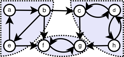
Graph with strongly connected components marked
## References
- [Wikipedia](https://en.wikipedia.org/wiki/Strongly_connected_component)
- [YouTube](https://www.youtube.com/watch?v=RpgcYiky7uw&list=PLLXdhg_r2hKA7DPDsunoDZ-Z769jWn4R8)
================================================
FILE: src/algorithms/graph/strongly-connected-components/__test__/stronglyConnectedComponents.test.js
================================================
import GraphVertex from '../../../../data-structures/graph/GraphVertex';
import GraphEdge from '../../../../data-structures/graph/GraphEdge';
import Graph from '../../../../data-structures/graph/Graph';
import stronglyConnectedComponents from '../stronglyConnectedComponents';
describe('stronglyConnectedComponents', () => {
it('should detect strongly connected components in simple graph', () => {
const vertexA = new GraphVertex('A');
const vertexB = new GraphVertex('B');
const vertexC = new GraphVertex('C');
const vertexD = new GraphVertex('D');
const edgeAB = new GraphEdge(vertexA, vertexB);
const edgeBC = new GraphEdge(vertexB, vertexC);
const edgeCA = new GraphEdge(vertexC, vertexA);
const edgeCD = new GraphEdge(vertexC, vertexD);
const graph = new Graph(true);
graph
.addEdge(edgeAB)
.addEdge(edgeBC)
.addEdge(edgeCA)
.addEdge(edgeCD);
const components = stronglyConnectedComponents(graph);
expect(components).toBeDefined();
expect(components.length).toBe(2);
expect(components[0][0].getKey()).toBe(vertexA.getKey());
expect(components[0][1].getKey()).toBe(vertexC.getKey());
expect(components[0][2].getKey()).toBe(vertexB.getKey());
expect(components[1][0].getKey()).toBe(vertexD.getKey());
});
it('should detect strongly connected components in graph', () => {
const vertexA = new GraphVertex('A');
const vertexB = new GraphVertex('B');
const vertexC = new GraphVertex('C');
const vertexD = new GraphVertex('D');
const vertexE = new GraphVertex('E');
const vertexF = new GraphVertex('F');
const vertexG = new GraphVertex('G');
const vertexH = new GraphVertex('H');
const vertexI = new GraphVertex('I');
const vertexJ = new GraphVertex('J');
const vertexK = new GraphVertex('K');
const edgeAB = new GraphEdge(vertexA, vertexB);
const edgeBC = new GraphEdge(vertexB, vertexC);
const edgeCA = new GraphEdge(vertexC, vertexA);
const edgeBD = new GraphEdge(vertexB, vertexD);
const edgeDE = new GraphEdge(vertexD, vertexE);
const edgeEF = new GraphEdge(vertexE, vertexF);
const edgeFD = new GraphEdge(vertexF, vertexD);
const edgeGF = new GraphEdge(vertexG, vertexF);
const edgeGH = new GraphEdge(vertexG, vertexH);
const edgeHI = new GraphEdge(vertexH, vertexI);
const edgeIJ = new GraphEdge(vertexI, vertexJ);
const edgeJG = new GraphEdge(vertexJ, vertexG);
const edgeJK = new GraphEdge(vertexJ, vertexK);
const graph = new Graph(true);
graph
.addEdge(edgeAB)
.addEdge(edgeBC)
.addEdge(edgeCA)
.addEdge(edgeBD)
.addEdge(edgeDE)
.addEdge(edgeEF)
.addEdge(edgeFD)
.addEdge(edgeGF)
.addEdge(edgeGH)
.addEdge(edgeHI)
.addEdge(edgeIJ)
.addEdge(edgeJG)
.addEdge(edgeJK);
const components = stronglyConnectedComponents(graph);
expect(components).toBeDefined();
expect(components.length).toBe(4);
expect(components[0][0].getKey()).toBe(vertexG.getKey());
expect(components[0][1].getKey()).toBe(vertexJ.getKey());
expect(components[0][2].getKey()).toBe(vertexI.getKey());
expect(components[0][3].getKey()).toBe(vertexH.getKey());
expect(components[1][0].getKey()).toBe(vertexK.getKey());
expect(components[2][0].getKey()).toBe(vertexA.getKey());
expect(components[2][1].getKey()).toBe(vertexC.getKey());
expect(components[2][2].getKey()).toBe(vertexB.getKey());
expect(components[3][0].getKey()).toBe(vertexD.getKey());
expect(components[3][1].getKey()).toBe(vertexF.getKey());
expect(components[3][2].getKey()).toBe(vertexE.getKey());
});
});
================================================
FILE: src/algorithms/graph/strongly-connected-components/stronglyConnectedComponents.js
================================================
import Stack from '../../../data-structures/stack/Stack';
import depthFirstSearch from '../depth-first-search/depthFirstSearch';
/**
* @param {Graph} graph
* @return {Stack}
*/
function getVerticesSortedByDfsFinishTime(graph) {
// Set of all visited vertices during DFS pass.
const visitedVerticesSet = {};
// Stack of vertices by finish time.
// All vertices in this stack are ordered by finished time in decreasing order.
// Vertex that has been finished first will be at the bottom of the stack and
// vertex that has been finished last will be at the top of the stack.
const verticesByDfsFinishTime = new Stack();
// Set of all vertices we're going to visit.
const notVisitedVerticesSet = {};
graph.getAllVertices().forEach((vertex) => {
notVisitedVerticesSet[vertex.getKey()] = vertex;
});
// Specify DFS traversal callbacks.
const dfsCallbacks = {
enterVertex: ({ currentVertex }) => {
// Add current vertex to visited set.
visitedVerticesSet[currentVertex.getKey()] = currentVertex;
// Delete current vertex from not visited set.
delete notVisitedVerticesSet[currentVertex.getKey()];
},
leaveVertex: ({ currentVertex }) => {
// Push vertex to the stack when leaving it.
// This will make stack to be ordered by finish time in decreasing order.
verticesByDfsFinishTime.push(currentVertex);
},
allowTraversal: ({ nextVertex }) => {
// Don't allow to traverse the nodes that have been already visited.
return !visitedVerticesSet[nextVertex.getKey()];
},
};
// Do FIRST DFS PASS traversal for all graph vertices to fill the verticesByFinishTime stack.
while (Object.values(notVisitedVerticesSet).length) {
// Peek any vertex to start DFS traversal from.
const startVertexKey = Object.keys(notVisitedVerticesSet)[0];
const startVertex = notVisitedVerticesSet[startVertexKey];
delete notVisitedVerticesSet[startVertexKey];
depthFirstSearch(graph, startVertex, dfsCallbacks);
}
return verticesByDfsFinishTime;
}
/**
* @param {Graph} graph
* @param {Stack} verticesByFinishTime
* @return {*[]}
*/
function getSCCSets(graph, verticesByFinishTime) {
// Array of arrays of strongly connected vertices.
const stronglyConnectedComponentsSets = [];
// Array that will hold all vertices that are being visited during one DFS run.
let stronglyConnectedComponentsSet = [];
// Visited vertices set.
const visitedVerticesSet = {};
// Callbacks for DFS traversal.
const dfsCallbacks = {
enterVertex: ({ currentVertex }) => {
// Add current vertex to SCC set of current DFS round.
stronglyConnectedComponentsSet.push(currentVertex);
// Add current vertex to visited set.
visitedVerticesSet[currentVertex.getKey()] = currentVertex;
},
leaveVertex: ({ previousVertex }) => {
// Once DFS traversal is finished push the set of found strongly connected
// components during current DFS round to overall strongly connected components set.
// The sign that traversal is about to be finished is that we came back to start vertex
// which doesn't have parent.
if (previousVertex === null) {
stronglyConnectedComponentsSets.push([...stronglyConnectedComponentsSet]);
}
},
allowTraversal: ({ nextVertex }) => {
// Don't allow traversal of already visited vertices.
return !visitedVerticesSet[nextVertex.getKey()];
},
};
while (!verticesByFinishTime.isEmpty()) {
/** @var {GraphVertex} startVertex */
const startVertex = verticesByFinishTime.pop();
// Reset the set of strongly connected vertices.
stronglyConnectedComponentsSet = [];
// Don't do DFS on already visited vertices.
if (!visitedVerticesSet[startVertex.getKey()]) {
// Do DFS traversal.
depthFirstSearch(graph, startVertex, dfsCallbacks);
}
}
return stronglyConnectedComponentsSets;
}
/**
* Kosaraju's algorithm.
*
* @param {Graph} graph
* @return {*[]}
*/
export default function stronglyConnectedComponents(graph) {
// In this algorithm we will need to do TWO DFS PASSES overt the graph.
// Get stack of vertices ordered by DFS finish time.
// All vertices in this stack are ordered by finished time in decreasing order:
// Vertex that has been finished first will be at the bottom of the stack and
// vertex that has been finished last will be at the top of the stack.
const verticesByFinishTime = getVerticesSortedByDfsFinishTime(graph);
// Reverse the graph.
graph.reverse();
// Do DFS once again on reversed graph.
return getSCCSets(graph, verticesByFinishTime);
}
================================================
FILE: src/algorithms/graph/topological-sorting/README.md
================================================
# Topological Sorting
In the field of computer science, a topological sort or
topological ordering of a directed graph is a linear ordering
of its vertices such that for every directed edge `uv` from
vertex `u` to vertex `v`, `u` comes before `v` in the ordering.
For instance, the vertices of the graph may represent tasks to
be performed, and the edges may represent constraints that one
task must be performed before another; in this application, a
topological ordering is just a valid sequence for the tasks.
A topological ordering is possible if and only if the graph has
no directed cycles, that is, if it is a [directed acyclic graph](https://en.wikipedia.org/wiki/Directed_acyclic_graph)
(DAG). Any DAG has at least one topological ordering, and algorithms are
known for constructing a topological ordering of any DAG in linear time.

A topological ordering of a directed acyclic graph: every edge goes from
earlier in the ordering (upper left) to later in the ordering (lower right).
A directed graph is acyclic if and only if it has a topological ordering.
## Example

The graph shown above has many valid topological sorts, including:
- `5, 7, 3, 11, 8, 2, 9, 10` (visual left-to-right, top-to-bottom)
- `3, 5, 7, 8, 11, 2, 9, 10` (smallest-numbered available vertex first)
- `5, 7, 3, 8, 11, 10, 9, 2` (fewest edges first)
- `7, 5, 11, 3, 10, 8, 9, 2` (largest-numbered available vertex first)
- `5, 7, 11, 2, 3, 8, 9, 10` (attempting top-to-bottom, left-to-right)
- `3, 7, 8, 5, 11, 10, 2, 9` (arbitrary)
## Application
The canonical application of topological sorting is in
**scheduling a sequence of jobs** or tasks based on their dependencies. The jobs
are represented by vertices, and there is an edge from `x` to `y` if
job `x` must be completed before job `y` can be started (for
example, when washing clothes, the washing machine must finish
before we put the clothes in the dryer). Then, a topological sort
gives an order in which to perform the jobs.
Other application is **dependency resolution**. Each vertex is a package
and each edge is a dependency of package `a` on package 'b'. Then topological
sorting will provide a sequence of installing dependencies in a way that every
next dependency has its dependent packages to be installed in prior.
## References
- [Wikipedia](https://en.wikipedia.org/wiki/Topological_sorting)
- [Topological Sorting on YouTube by Tushar Roy](https://www.youtube.com/watch?v=ddTC4Zovtbc&list=PLLXdhg_r2hKA7DPDsunoDZ-Z769jWn4R8)
================================================
FILE: src/algorithms/graph/topological-sorting/__test__/topologicalSort.test.js
================================================
import GraphVertex from '../../../../data-structures/graph/GraphVertex';
import GraphEdge from '../../../../data-structures/graph/GraphEdge';
import Graph from '../../../../data-structures/graph/Graph';
import topologicalSort from '../topologicalSort';
describe('topologicalSort', () => {
it('should do topological sorting on graph', () => {
const vertexA = new GraphVertex('A');
const vertexB = new GraphVertex('B');
const vertexC = new GraphVertex('C');
const vertexD = new GraphVertex('D');
const vertexE = new GraphVertex('E');
const vertexF = new GraphVertex('F');
const vertexG = new GraphVertex('G');
const vertexH = new GraphVertex('H');
const edgeAC = new GraphEdge(vertexA, vertexC);
const edgeBC = new GraphEdge(vertexB, vertexC);
const edgeBD = new GraphEdge(vertexB, vertexD);
const edgeCE = new GraphEdge(vertexC, vertexE);
const edgeDF = new GraphEdge(vertexD, vertexF);
const edgeEF = new GraphEdge(vertexE, vertexF);
const edgeEH = new GraphEdge(vertexE, vertexH);
const edgeFG = new GraphEdge(vertexF, vertexG);
const graph = new Graph(true);
graph
.addEdge(edgeAC)
.addEdge(edgeBC)
.addEdge(edgeBD)
.addEdge(edgeCE)
.addEdge(edgeDF)
.addEdge(edgeEF)
.addEdge(edgeEH)
.addEdge(edgeFG);
const sortedVertices = topologicalSort(graph);
expect(sortedVertices).toBeDefined();
expect(sortedVertices.length).toBe(graph.getAllVertices().length);
expect(sortedVertices).toEqual([
vertexB,
vertexD,
vertexA,
vertexC,
vertexE,
vertexH,
vertexF,
vertexG,
]);
});
});
================================================
FILE: src/algorithms/graph/topological-sorting/topologicalSort.js
================================================
import Stack from '../../../data-structures/stack/Stack';
import depthFirstSearch from '../depth-first-search/depthFirstSearch';
/**
* @param {Graph} graph
*/
export default function topologicalSort(graph) {
// Create a set of all vertices we want to visit.
const unvisitedSet = {};
graph.getAllVertices().forEach((vertex) => {
unvisitedSet[vertex.getKey()] = vertex;
});
// Create a set for all vertices that we've already visited.
const visitedSet = {};
// Create a stack of already ordered vertices.
const sortedStack = new Stack();
const dfsCallbacks = {
enterVertex: ({ currentVertex }) => {
// Add vertex to visited set in case if all its children has been explored.
visitedSet[currentVertex.getKey()] = currentVertex;
// Remove this vertex from unvisited set.
delete unvisitedSet[currentVertex.getKey()];
},
leaveVertex: ({ currentVertex }) => {
// If the vertex has been totally explored then we may push it to stack.
sortedStack.push(currentVertex);
},
allowTraversal: ({ nextVertex }) => {
return !visitedSet[nextVertex.getKey()];
},
};
// Let's go and do DFS for all unvisited nodes.
while (Object.keys(unvisitedSet).length) {
const currentVertexKey = Object.keys(unvisitedSet)[0];
const currentVertex = unvisitedSet[currentVertexKey];
// Do DFS for current node.
depthFirstSearch(graph, currentVertex, dfsCallbacks);
}
return sortedStack.toArray();
}
================================================
FILE: src/algorithms/graph/travelling-salesman/README.md
================================================
# Travelling Salesman Problem
The travelling salesman problem (TSP) asks the following question:
"Given a list of cities and the distances between each pair of
cities, what is the shortest possible route that visits each city
and returns to the origin city?"

Solution of a travelling salesman problem: the black line shows
the shortest possible loop that connects every red dot.

TSP can be modelled as an undirected weighted graph, such that
cities are the graph's vertices, paths are the graph's edges,
and a path's distance is the edge's weight. It is a minimization
problem starting and finishing at a specified vertex after having
visited each other vertex exactly once. Often, the model is a
complete graph (i.e. each pair of vertices is connected by an
edge). If no path exists between two cities, adding an arbitrarily
long edge will complete the graph without affecting the optimal tour.
## References
- [Wikipedia](https://en.wikipedia.org/wiki/Travelling_salesman_problem)
================================================
FILE: src/algorithms/graph/travelling-salesman/__test__/bfTravellingSalesman.test.js
================================================
import GraphVertex from '../../../../data-structures/graph/GraphVertex';
import GraphEdge from '../../../../data-structures/graph/GraphEdge';
import Graph from '../../../../data-structures/graph/Graph';
import bfTravellingSalesman from '../bfTravellingSalesman';
describe('bfTravellingSalesman', () => {
it('should solve problem for simple graph', () => {
const vertexA = new GraphVertex('A');
const vertexB = new GraphVertex('B');
const vertexC = new GraphVertex('C');
const vertexD = new GraphVertex('D');
const edgeAB = new GraphEdge(vertexA, vertexB, 1);
const edgeBD = new GraphEdge(vertexB, vertexD, 1);
const edgeDC = new GraphEdge(vertexD, vertexC, 1);
const edgeCA = new GraphEdge(vertexC, vertexA, 1);
const edgeBA = new GraphEdge(vertexB, vertexA, 5);
const edgeDB = new GraphEdge(vertexD, vertexB, 8);
const edgeCD = new GraphEdge(vertexC, vertexD, 7);
const edgeAC = new GraphEdge(vertexA, vertexC, 4);
const edgeAD = new GraphEdge(vertexA, vertexD, 2);
const edgeDA = new GraphEdge(vertexD, vertexA, 3);
const edgeBC = new GraphEdge(vertexB, vertexC, 3);
const edgeCB = new GraphEdge(vertexC, vertexB, 9);
const graph = new Graph(true);
graph
.addEdge(edgeAB)
.addEdge(edgeBD)
.addEdge(edgeDC)
.addEdge(edgeCA)
.addEdge(edgeBA)
.addEdge(edgeDB)
.addEdge(edgeCD)
.addEdge(edgeAC)
.addEdge(edgeAD)
.addEdge(edgeDA)
.addEdge(edgeBC)
.addEdge(edgeCB);
const salesmanPath = bfTravellingSalesman(graph);
expect(salesmanPath.length).toBe(4);
expect(salesmanPath[0].getKey()).toEqual(vertexA.getKey());
expect(salesmanPath[1].getKey()).toEqual(vertexB.getKey());
expect(salesmanPath[2].getKey()).toEqual(vertexD.getKey());
expect(salesmanPath[3].getKey()).toEqual(vertexC.getKey());
});
});
================================================
FILE: src/algorithms/graph/travelling-salesman/bfTravellingSalesman.js
================================================
/**
* Get all possible paths
* @param {GraphVertex} startVertex
* @param {GraphVertex[][]} [paths]
* @param {GraphVertex[]} [path]
*/
function findAllPaths(startVertex, paths = [], path = []) {
// Clone path.
const currentPath = [...path];
// Add startVertex to the path.
currentPath.push(startVertex);
// Generate visited set from path.
const visitedSet = currentPath.reduce((accumulator, vertex) => {
const updatedAccumulator = { ...accumulator };
updatedAccumulator[vertex.getKey()] = vertex;
return updatedAccumulator;
}, {});
// Get all unvisited neighbors of startVertex.
const unvisitedNeighbors = startVertex.getNeighbors().filter((neighbor) => {
return !visitedSet[neighbor.getKey()];
});
// If there no unvisited neighbors then treat current path as complete and save it.
if (!unvisitedNeighbors.length) {
paths.push(currentPath);
return paths;
}
// Go through all the neighbors.
for (let neighborIndex = 0; neighborIndex < unvisitedNeighbors.length; neighborIndex += 1) {
const currentUnvisitedNeighbor = unvisitedNeighbors[neighborIndex];
findAllPaths(currentUnvisitedNeighbor, paths, currentPath);
}
return paths;
}
/**
* @param {number[][]} adjacencyMatrix
* @param {object} verticesIndices
* @param {GraphVertex[]} cycle
* @return {number}
*/
function getCycleWeight(adjacencyMatrix, verticesIndices, cycle) {
let weight = 0;
for (let cycleIndex = 1; cycleIndex < cycle.length; cycleIndex += 1) {
const fromVertex = cycle[cycleIndex - 1];
const toVertex = cycle[cycleIndex];
const fromVertexIndex = verticesIndices[fromVertex.getKey()];
const toVertexIndex = verticesIndices[toVertex.getKey()];
weight += adjacencyMatrix[fromVertexIndex][toVertexIndex];
}
return weight;
}
/**
* BRUTE FORCE approach to solve Traveling Salesman Problem.
*
* @param {Graph} graph
* @return {GraphVertex[]}
*/
export default function bfTravellingSalesman(graph) {
// Pick starting point from where we will traverse the graph.
const startVertex = graph.getAllVertices()[0];
// BRUTE FORCE.
// Generate all possible paths from startVertex.
const allPossiblePaths = findAllPaths(startVertex);
// Filter out paths that are not cycles.
const allPossibleCycles = allPossiblePaths.filter((path) => {
/** @var {GraphVertex} */
const lastVertex = path[path.length - 1];
const lastVertexNeighbors = lastVertex.getNeighbors();
return lastVertexNeighbors.includes(startVertex);
});
// Go through all possible cycles and pick the one with minimum overall tour weight.
const adjacencyMatrix = graph.getAdjacencyMatrix();
const verticesIndices = graph.getVerticesIndices();
let salesmanPath = [];
let salesmanPathWeight = null;
for (let cycleIndex = 0; cycleIndex < allPossibleCycles.length; cycleIndex += 1) {
const currentCycle = allPossibleCycles[cycleIndex];
const currentCycleWeight = getCycleWeight(adjacencyMatrix, verticesIndices, currentCycle);
// If current cycle weight is smaller then previous ones treat current cycle as most optimal.
if (salesmanPathWeight === null || currentCycleWeight < salesmanPathWeight) {
salesmanPath = currentCycle;
salesmanPathWeight = currentCycleWeight;
}
}
// Return the solution.
return salesmanPath;
}
================================================
FILE: src/algorithms/image-processing/seam-carving/README.md
================================================
# Content-aware image resizing in JavaScript

> There is an [interactive version of this post](https://trekhleb.dev/blog/2021/content-aware-image-resizing-in-javascript/) available where you can upload and resize your custom images.
## TL;DR
There are many great articles written about the *Seam Carving algorithm* already, but I couldn't resist the temptation to explore this elegant, powerful, and *yet simple* algorithm on my own, and to write about my personal experience with it. Another point that drew my attention (as a creator of [javascript-algorithms](https://github.com/trekhleb/javascript-algorithms) repo) was the fact that *Dynamic Programming (DP)* approach might be smoothly applied to solve it. And, if you're like me and still on your "learning algorithms" journey, this algorithmic solution may enrich your personal DP arsenal.
So, with this article I want to do three things:
1. Provide you with an interactive **content-aware resizer** so that you could play around with resizing your own images
2. Explain the idea behind the **Seam Carving algorithm**
3. Explain the **dynamic programming approach** to implement the algorithm (we'll be using TypeScript for it)
### Content-aware image resizing
*Content-aware image resizing* might be applied when it comes to changing the image proportions (i.e. reducing the width while keeping the height) and when losing some parts of the image is not desirable. Doing the straightforward image scaling in this case would distort the objects in it. To preserve the proportions of the objects while changing the image proportions we may use the [Seam Carving algorithm](https://perso.crans.org/frenoy/matlab2012/seamcarving.pdf) that was introduced by *Shai Avidan* and *Ariel Shamir*.
The example below shows how the original image width was reduced by 50% using *content-aware resizing* (left image) and *straightforward scaling* (right image). In this particular case, the left image looks more natural since the proportions of the balloons were preserved.

The Seam Carving algorithm's idea is to find the *seam* (continuous sequence of pixels) with the lowest contribution to the image content and then *carve* (remove) it. This process repeats over and over again until we get the required image width or height. In the example below you may see that the hot air balloon pixels contribute more to the content of the image than the sky pixels. Thus, the sky pixels are being removed first.

Finding the seam with the lowest energy is a computationally expensive task (especially for large images). To make the seam search faster the *dynamic programming* approach might be applied (we will go through the implementation details below).
### Objects removal
The importance of each pixel (so-called pixel's energy) is being calculated based on its color (`R`, `G`, `B`, `A`) difference between two neighbor pixels. Now, if we set the pixel energy to some really low level artificially (i.e. by drawing a mask on top of them), the Seam Carving algorithm would perform an **object removal** for us for free.

### JS IMAGE CARVER demo
I've created the [JS IMAGE CARVER](https://trekhleb.dev/js-image-carver/) web-app (and also [open-sourced it on GitHub](https://github.com/trekhleb/js-image-carver)) that you may use to play around with resizing of your custom images.
### More examples
Here are some more examples of how the algorithm copes with more complex backgrounds.
Mountains on the background are being shrunk smoothly without visible seams.

The same goes for the ocean waves. The algorithm preserved the wave structure without distorting the surfers.

We need to keep in mind that the Seam Carving algorithm is not a silver bullet, and it may fail to resize the images where *most of the pixels are edges* (look important to the algorithm). In this case, it starts distorting even the important parts of the image. In the example below the content-aware image resizing looks pretty similar to a straightforward scaling since for the algorithm all the pixels look important, and it is hard for it to distinguish Van Gogh's face from the background.

## How Seam Carving algorithms works
Imagine we have a `1000 x 500 px` picture, and we want to change its size to `500 x 500 px` to make it square (let's say the square ratio would better fit the Instagram feed). We might want to set up several **requirements to the resizing process** in this case:
- *Preserve the important parts of the image* (i.e. if there were 5 trees before the resizing we want to have 5 trees after resizing as well).
- *Preserve the proportions* of the important parts of the image (i.e. circle car wheels should not be squeezed to the ellipse wheels)
To avoid changing the important parts of the image we may find the **continuous sequence of pixels (the seam)**, that goes from top to bottom and has *the lowest contribution to the content* of the image (avoids important parts) and then remove it. The seam removal will shrink the image by 1 pixel. We will then repeat this step until the image will get the desired width.
The question is how to define *the importance of the pixel* and its contribution to the content (in the original paper the authors are using the term **energy of the pixel**). One of the ways to do it is to treat all the pixels that form the edges as important ones. In case if a pixel is a part of the edge its color would have a greater difference between the neighbors (left and right pixels) than the pixel that isn't a part of the edge.
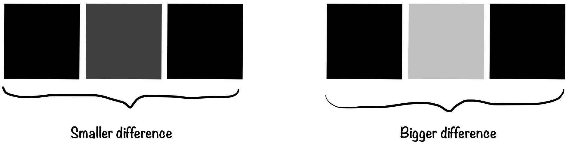
Assuming that the color of a pixel is represented by *4* numbers (`R` - red, `G` - green, `B` - blue, `A` - alpha) we may use the following formula to calculate the color difference (the pixel energy):

Where:
- `mEnergy` - *Energy* (importance) of the *middle* pixel (`[0..626]` if rounded)
- `lR` - *Red* channel value for the *left* pixel (`[0..255]`)
- `mR` - *Red* channel value for the *middle* pixel (`[0..255]`)
- `rR` - *Red* channel value for the *right* pixel (`[0..255]`)
- `lG` - *Green* channel value for the *left* pixel (`[0..255]`)
- and so on...
In the formula above we're omitting the alpha (transparency) channel, for now, assuming that there are no transparent pixels in the image. Later we will use the alpha channel for masking and for object removal.
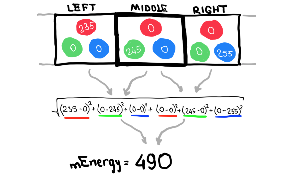
Now, since we know how to find the energy of one pixel, we can calculate, so-called, **energy map** which will contain the energies of each pixel of the image. On each resizing step the energy map should be re-calculated (at least partially, more about it below) and would have the same size as the image.
For example, on the 1st resizing step we will have a `1000 x 500` image and a `1000 x 500` energy map. On the 2nd resizing step we will remove the seam from the image and re-calculate the energy map based on the new shrunk image. Thus, we will get a `999 x 500` image and a `999 x 500` energy map.
The higher the energy of the pixel the more likely it is a part of an edge, and it is important for the image content and the less likely that we need to remove it.
To visualize the energy map we may assign a brighter color to the pixels with the higher energy and darker colors to the pixels with the lower energy. Here is an artificial example of how the random part of the energy map might look like. You may see the bright line which represents the edge and which we want to preserve during the resizing.
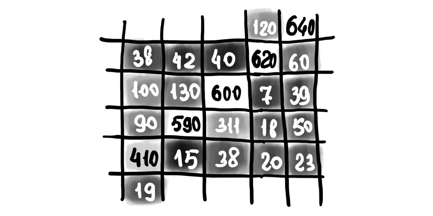
Here is a real example of the energy map for the demo image you saw above (with hot air balloons).

You may play around with your custom images and see how the energy map would look like in the [interactive version of the post](https://trekhleb.dev/blog/2021/content-aware-image-resizing-in-javascript/).
We may use the energy map to find the seams (one after another) with the lowest energy and by doing this to decide which pixels should be ultimately deleted.
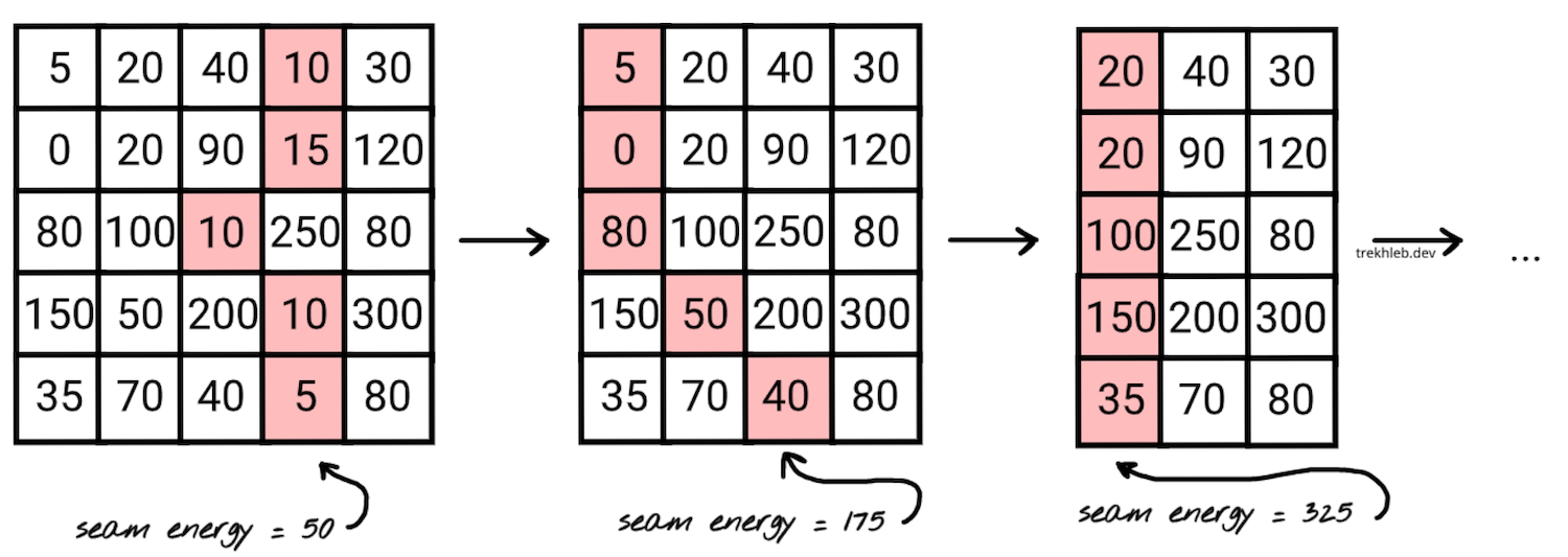
Finding the seam with the lowest energy is not a trivial task and requires exploring many possible pixel combinations before making the decision. We will apply the dynamic programming approach to speed it up.
In the example below, you may see the energy map with the first lowest energy seam that was found for it.

In the examples above we were reducing the width of the image. A similar approach may be taken to reduce the image height. We need to "rotate" the approach though:
- start using *top* and *bottom* pixel neighbors (instead of *left* and *right* ones) to calculate the pixel energy
- when searching for a seam we need to move from *left* to *right* (instead of from *up* to *bottom*)
## Implementation in TypeScript
> You may find the source code, and the functions mentioned below in the [js-image-carver](https://github.com/trekhleb/js-image-carver) repository.
To implement the algorithm we will be using TypeScript. If you want a JavaScript version, you may ignore (remove) type definitions and their usages.
For simplicity reasons let's implement the seam carving algorithm only for the image *width* reduction.
### Content-aware width resizing (the entry function)
First, let's define some common types that we're going to use while implementing the algorithm.
```typescript
// Type that describes the image size (width and height).
type ImageSize = { w: number, h: number };
// The coordinate of the pixel.
type Coordinate = { x: number, y: number };
// The seam is a sequence of pixels (coordinates).
type Seam = Coordinate[];
// Energy map is a 2D array that has the same width and height
// as the image the map is being calculated for.
type EnergyMap = number[][];
// Type that describes the image pixel's RGBA color.
type Color = [
r: number, // Red
g: number, // Green
b: number, // Blue
a: number, // Alpha (transparency)
] | Uint8ClampedArray;
```
On the high level the algorithm consists of the following steps:
1. Calculate the **energy map** for the current version of the image.
2. Find the **seam** with the lowest energy based on the energy map (this is where we will apply Dynamic Programming).
3. **Delete the seam** with the lowest energy seam from the image.
4. **Repeat** until the image width is reduced to the desired value.
```typescript
type ResizeImageWidthArgs = {
img: ImageData, // Image data we want to resize.
toWidth: number, // Final image width we want the image to shrink to.
};
type ResizeImageWidthResult = {
img: ImageData, // Resized image data.
size: ImageSize, // Resized image size (w x h).
};
// Performs the content-aware image width resizing using the seam carving method.
export const resizeImageWidth = (
{ img, toWidth }: ResizeImageWidthArgs,
): ResizeImageWidthResult => {
// For performance reasons we want to avoid changing the img data array size.
// Instead we'll just keep the record of the resized image width and height separately.
const size: ImageSize = { w: img.width, h: img.height };
// Calculating the number of pixels to remove.
const pxToRemove = img.width - toWidth;
if (pxToRemove < 0) {
throw new Error('Upsizing is not supported for now');
}
let energyMap: EnergyMap | null = null;
let seam: Seam | null = null;
// Removing the lowest energy seams one by one.
for (let i = 0; i < pxToRemove; i += 1) {
// 1. Calculate the energy map for the current version of the image.
energyMap = calculateEnergyMap(img, size);
// 2. Find the seam with the lowest energy based on the energy map.
seam = findLowEnergySeam(energyMap, size);
// 3. Delete the seam with the lowest energy seam from the image.
deleteSeam(img, seam, size);
// Reduce the image width, and continue iterations.
size.w -= 1;
}
// Returning the resized image and its final size.
// The img is actually a reference to the ImageData, so technically
// the caller of the function already has this pointer. But let's
// still return it for better code readability.
return { img, size };
};
```
The image that needs to be resized is being passed to the function in [ImageData](https://developer.mozilla.org/en-US/docs/Web/API/ImageData) format. You may draw the image on the canvas and then extract the ImageData from the canvas like this:
```javascript
const ctx = canvas.getContext('2d');
const imgData = ctx.getImageData(0, 0, imgWidth, imgHeight);
```
> The way of uploading and drawing images in JavaScript is out of scope for this article, but you may find the complete source code of how it may be done using React in [js-image-carver](https://github.com/trekhleb/js-image-carver) repo.
Let's break down each step ony be one and implement the `calculateEnergyMap()`, `findLowEnergySeam()` and `deleteSeam()` functions.
### Calculating the pixel's energy
Here we apply the color difference formula described above. For the left and right borders (when there are no left or right neighbors), we ignore the neighbors and don't take them into account during the energy calculation.
```typescript
// Calculates the energy of a pixel.
const getPixelEnergy = (left: Color | null, middle: Color, right: Color | null): number => {
// Middle pixel is the pixel we're calculating the energy for.
const [mR, mG, mB] = middle;
// Energy from the left pixel (if it exists).
let lEnergy = 0;
if (left) {
const [lR, lG, lB] = left;
lEnergy = (lR - mR) ** 2 + (lG - mG) ** 2 + (lB - mB) ** 2;
}
// Energy from the right pixel (if it exists).
let rEnergy = 0;
if (right) {
const [rR, rG, rB] = right;
rEnergy = (rR - mR) ** 2 + (rG - mG) ** 2 + (rB - mB) ** 2;
}
// Resulting pixel energy.
return Math.sqrt(lEnergy + rEnergy);
};
```
### Calculating the energy map
The image we're working with has the [ImageData](https://developer.mozilla.org/en-US/docs/Web/API/ImageData) format. It means that all the pixels (and their colors) are stored in a flat (*1D*) [Uint8ClampedArray](https://developer.mozilla.org/en-US/docs/Web/JavaScript/Reference/Global_Objects/Uint8ClampedArray) array. For readability purposes let's introduce the couple of helper functions that will allow us to work with the Uint8ClampedArray array as with a *2D* matrix instead.
```typescript
// Helper function that returns the color of the pixel.
const getPixel = (img: ImageData, { x, y }: Coordinate): Color => {
// The ImageData data array is a flat 1D array.
// Thus we need to convert x and y coordinates to the linear index.
const i = y * img.width + x;
const cellsPerColor = 4; // RGBA
// For better efficiency, instead of creating a new sub-array we return
// a pointer to the part of the ImageData array.
return img.data.subarray(i * cellsPerColor, i * cellsPerColor + cellsPerColor);
};
// Helper function that sets the color of the pixel.
const setPixel = (img: ImageData, { x, y }: Coordinate, color: Color): void => {
// The ImageData data array is a flat 1D array.
// Thus we need to convert x and y coordinates to the linear index.
const i = y * img.width + x;
const cellsPerColor = 4; // RGBA
img.data.set(color, i * cellsPerColor);
};
```
To calculate the energy map we go through each image pixel and call the previously described `getPixelEnergy()` function against it.
```typescript
// Helper function that creates a matrix (2D array) of specific
// size (w x h) and fills it with specified value.
const matrix = (w: number, h: number, filler: T): T[][] => {
return new Array(h)
.fill(null)
.map(() => {
return new Array(w).fill(filler);
});
};
// Calculates the energy of each pixel of the image.
const calculateEnergyMap = (img: ImageData, { w, h }: ImageSize): EnergyMap => {
// Create an empty energy map where each pixel has infinitely high energy.
// We will update the energy of each pixel.
const energyMap: number[][] = matrix(w, h, Infinity);
for (let y = 0; y < h; y += 1) {
for (let x = 0; x < w; x += 1) {
// Left pixel might not exist if we're on the very left edge of the image.
const left = (x - 1) >= 0 ? getPixel(img, { x: x - 1, y }) : null;
// The color of the middle pixel that we're calculating the energy for.
const middle = getPixel(img, { x, y });
// Right pixel might not exist if we're on the very right edge of the image.
const right = (x + 1) < w ? getPixel(img, { x: x + 1, y }) : null;
energyMap[y][x] = getPixelEnergy(left, middle, right);
}
}
return energyMap;
};
```
> The energy map is going to be recalculated on every resize iteration. It means that it will be recalculated, let's say, 500 times if we need to shrink the image by 500 pixels which is not optimal. To speed up the energy map calculation on the 2nd, 3rd, and further steps, we may re-calculate the energy only for those pixels that are placed around the seam that is going to be removed. For simplicity reasons this optimization is omitted here, but you may find the example source-code in [js-image-carver](https://github.com/trekhleb/js-image-carver) repo.
### Finding the seam with the lowest energy (Dynamic Programming approach)
> I've described some Dynamic Programming basics in [Dynamic Programming vs Divide-and-Conquer](https://trekhleb.dev/blog/2018/dynamic-programming-vs-divide-and-conquer/) article before. There is a DP example based on the minimum edit distance problem. You might want to check it out to get some more context.
The issue we need to solve now is to find the path (the seam) on the energy map that goes from top to bottom and has the minimum sum of pixel energies.
#### The naive approach
The naive approach would be to check all possible paths one after another.
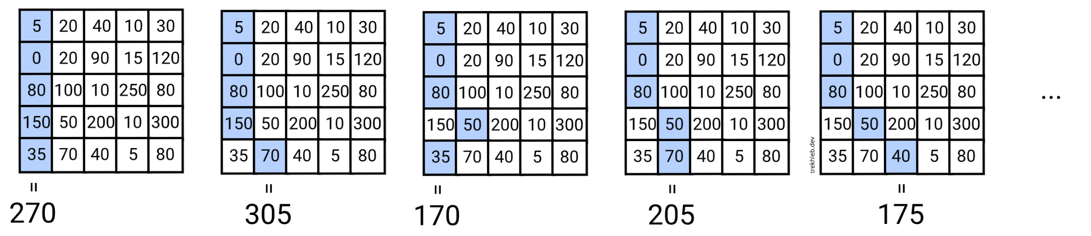
Going from top to bottom, for each pixel, we have 3 options (↙︎ go down-left, ↓ go down, ↘︎ go down-right). This gives us the time complexity of `O(w * 3^h)` or simply `O(3^h)`, where `w` and `h` are the width and the height of the image. This approach looks slow.
#### The greedy approach
We may also try to choose the next pixel as a pixel with the lowest energy, hoping that the resulting seam energy will be the smallest one.
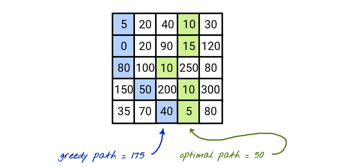
This approach gives not the worst solution, but it cannot guarantee that we will find the best available solution. On the image above you may see how the greedy approach chose `5` instead of `10` at first and missed the chain of optimal pixels.
The good part about this approach is that it is fast, and it has a time complexity of `O(w + h)`, where `w` and `h` are the width and the height of the image. In this case, the cost of the speed is the low quality of resizing. We need to find a minimum value in the first row (traversing `w` cells) and then we explore only 3 neighbor pixels for each row (traversing `h` rows).
#### The dynamic programming approach
You might have noticed that in the naive approach we summed up the same pixel energies over and over again while calculating the resulting seams' energy.
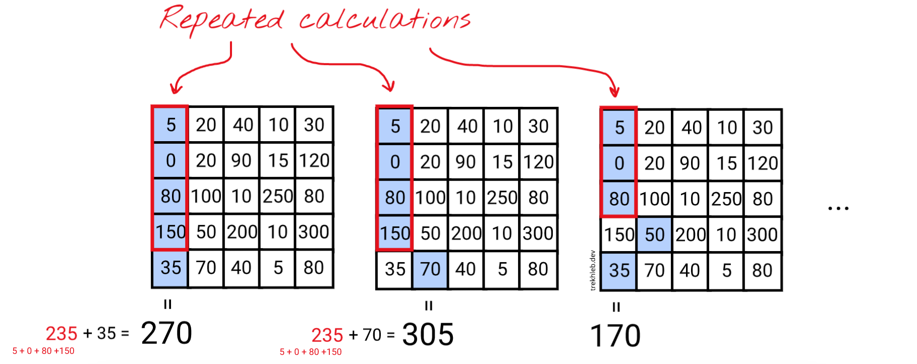
In the example above you see that for the first two seams we are re-using the energy of the shorter seam (which has the energy of `235`). Instead of doing just one operation `235 + 70` to calculate the energy of the 2nd seam we're doing four operations `(5 + 0 + 80 + 150) + 70`.
> This fact that we're re-using the energy of the previous seam to calculate the current seam's energy might be applied recursively to all the shorter seams up to the very top 1st row seam. When we have such overlapping sub-problems, [it is a sign](https://trekhleb.dev/blog/2018/dynamic-programming-vs-divide-and-conquer/) that the general problem *might* be optimized by dynamic programming approach.
So, we may **save the energy of the current seam** at the particular pixel in an additional `seamsEnergies` table to make it re-usable for calculating the next seams faster (the `seamsEnergies` table will have the same size as the energy map and the image itself).
Let's also keep in mind that for one particular pixel on the image (i.e. the bottom left one) we may have *several* values of the previous seams energies.
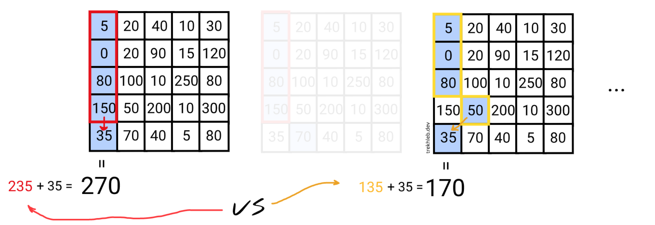
Since we're looking for a seam with the lowest resulting energy it would make sense to pick the previous seam with the lowest resulting energy as well.
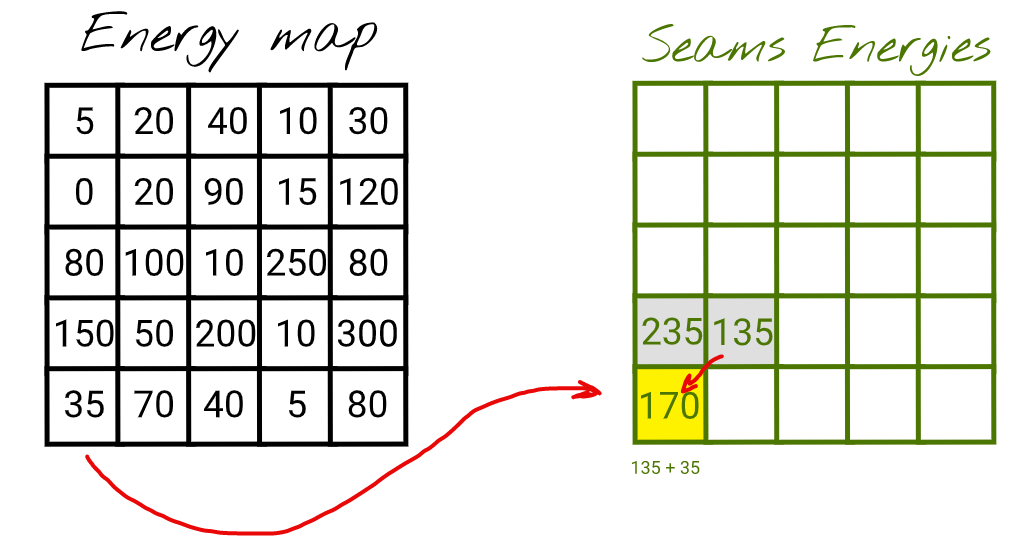
In general, we have three possible previous seems to choose from:
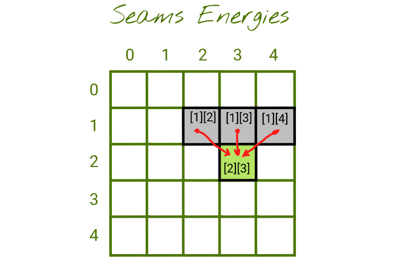
You may think about it this way:
- The cell `[1][x]`: contains the lowest possible energy of the seam that starts somewhere on the row `[0][?]` and ends up at cell `[1][x]`
- **The current cell** `[2][3]`: contains the lowest possible energy of the seam that starts somewhere on the row `[0][?]` and ends up at cell `[2][3]`. To calculate it we need to sum up the energy of the current pixel `[2][3]` (from the energy map) with the `min(seam_energy_1_2, seam_energy_1_3, seam_energy_1_4)`
If we fill the `seamsEnergies` table completely, then the minimum number in the lowest row would be the lowest possible seam energy.
Let's try to fill several cells of this table to see how it works.
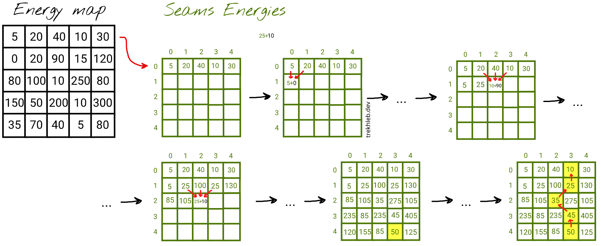
After filling out the `seamsEnergies` table we may see that the lowest energy pixel has an energy of `50`. For convenience, during the `seamsEnergies` generation for each pixel, we may save not only the energy of the seam but also the coordinates of the previous lowest energy seam. This will give us the possibility to reconstruct the seam path from the bottom to the top easily.
The time complexity of DP approach would be `O(w * h)`, where `w` and `h` are the width and the height of the image. We need to calculate energies for *every* pixel of the image.
Here is an example of how this logic might be implemented:
```typescript
// The metadata for the pixels in the seam.
type SeamPixelMeta = {
energy: number, // The energy of the pixel.
coordinate: Coordinate, // The coordinate of the pixel.
previous: Coordinate | null, // The previous pixel in a seam.
};
// Finds the seam (the sequence of pixels from top to bottom) that has the
// lowest resulting energy using the Dynamic Programming approach.
const findLowEnergySeam = (energyMap: EnergyMap, { w, h }: ImageSize): Seam => {
// The 2D array of the size of w and h, where each pixel contains the
// seam metadata (pixel energy, pixel coordinate and previous pixel from
// the lowest energy seam at this point).
const seamsEnergies: (SeamPixelMeta | null)[][] = matrix(w, h, null);
// Populate the first row of the map by just copying the energies
// from the energy map.
for (let x = 0; x < w; x += 1) {
const y = 0;
seamsEnergies[y][x] = {
energy: energyMap[y][x],
coordinate: { x, y },
previous: null,
};
}
// Populate the rest of the rows.
for (let y = 1; y < h; y += 1) {
for (let x = 0; x < w; x += 1) {
// Find the top adjacent cell with minimum energy.
// This cell would be the tail of a seam with lowest energy at this point.
// It doesn't mean that this seam (path) has lowest energy globally.
// Instead, it means that we found a path with the lowest energy that may lead
// us to the current pixel with the coordinates x and y.
let minPrevEnergy = Infinity;
let minPrevX: number = x;
for (let i = (x - 1); i <= (x + 1); i += 1) {
if (i >= 0 && i < w && seamsEnergies[y - 1][i].energy < minPrevEnergy) {
minPrevEnergy = seamsEnergies[y - 1][i].energy;
minPrevX = i;
}
}
// Update the current cell.
seamsEnergies[y][x] = {
energy: minPrevEnergy + energyMap[y][x],
coordinate: { x, y },
previous: { x: minPrevX, y: y - 1 },
};
}
}
// Find where the minimum energy seam ends.
// We need to find the tail of the lowest energy seam to start
// traversing it from its tail to its head (from the bottom to the top).
let lastMinCoordinate: Coordinate | null = null;
let minSeamEnergy = Infinity;
for (let x = 0; x < w; x += 1) {
const y = h - 1;
if (seamsEnergies[y][x].energy < minSeamEnergy) {
minSeamEnergy = seamsEnergies[y][x].energy;
lastMinCoordinate = { x, y };
}
}
// Find the lowest energy energy seam.
// Once we know where the tail is we may traverse and assemble the lowest
// energy seam based on the "previous" value of the seam pixel metadata.
const seam: Seam = [];
if (!lastMinCoordinate) {
return seam;
}
const { x: lastMinX, y: lastMinY } = lastMinCoordinate;
// Adding new pixel to the seam path one by one until we reach the top.
let currentSeam = seamsEnergies[lastMinY][lastMinX];
while (currentSeam) {
seam.push(currentSeam.coordinate);
const prevMinCoordinates = currentSeam.previous;
if (!prevMinCoordinates) {
currentSeam = null;
} else {
const { x: prevMinX, y: prevMinY } = prevMinCoordinates;
currentSeam = seamsEnergies[prevMinY][prevMinX];
}
}
return seam;
};
```
### Removing the seam with the lowest energy
Once we found the lowest energy seam, we need to remove (to carve) the pixels that form it from the image. The removal is happening by shifting the pixels to the right of the seam by `1px` to the left. For performance reasons, we don't actually delete the last columns. Instead, the rendering component will just ignore the part of the image that lays beyond the resized image width.
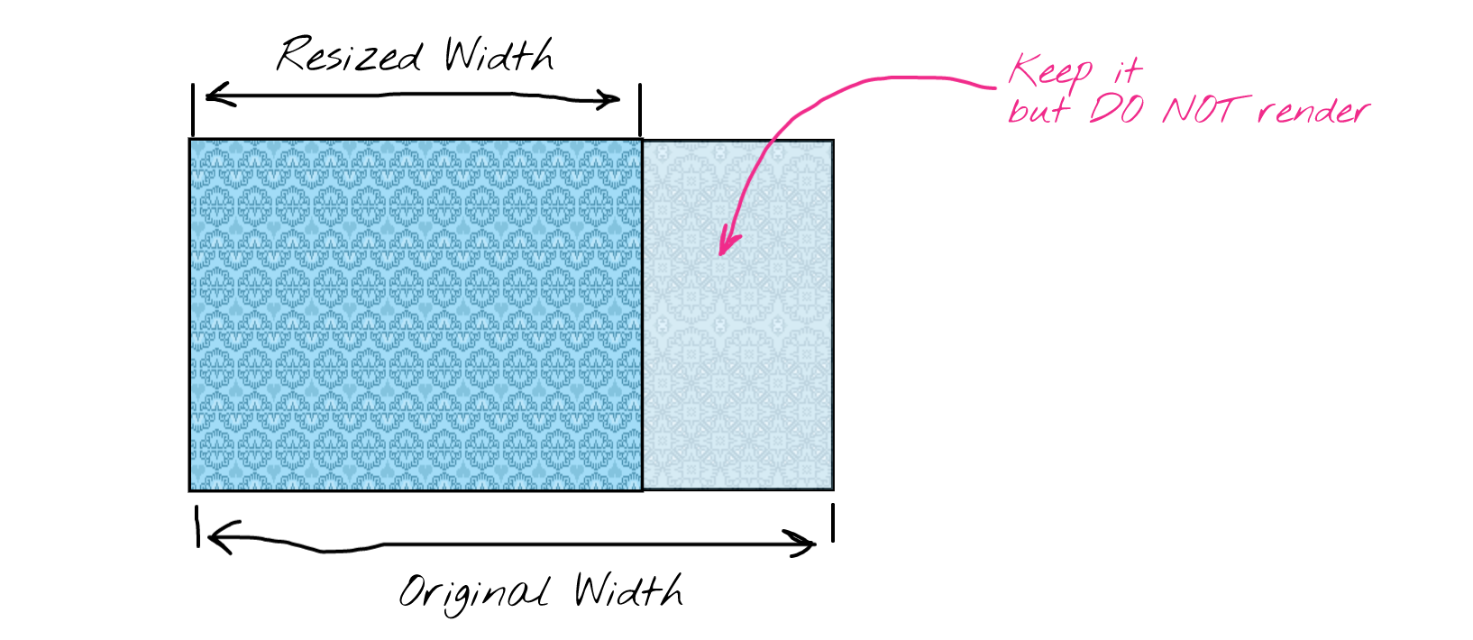
```typescript
// Deletes the seam from the image data.
// We delete the pixel in each row and then shift the rest of the row pixels to the left.
const deleteSeam = (img: ImageData, seam: Seam, { w }: ImageSize): void => {
seam.forEach(({ x: seamX, y: seamY }: Coordinate) => {
for (let x = seamX; x < (w - 1); x += 1) {
const nextPixel = getPixel(img, { x: x + 1, y: seamY });
setPixel(img, { x, y: seamY }, nextPixel);
}
});
};
```
## Objects removal
The Seam Carving algorithm tries to remove the seams which consist of low energy pixels first. We could leverage this fact and by assigning low energy to some pixels manually (i.e. by drawing on the image and masking out some areas of it) we could make the Seam Carving algorithm to do *objects removal* for us for free.
Currently, in `getPixelEnergy()` function we were using only the `R`, `G`, `B` color channels to calculate the pixel's energy. But there is also the `A` (alpha, transparency) parameter of the color that we didn't use yet. We may use the transparency channel to tell the algorithm that transparent pixels are the pixels we want to remove. You may check the [source-code of the energy function](https://github.com/trekhleb/js-image-carver/blob/main/src/utils/contentAwareResizer.ts#L54) that takes transparency into account.
Here is how the algorithm works for object removal.

## Issues and what's next
The [JS IMAGE CARVER](https://github.com/trekhleb/js-image-carver) web app is far from being a production ready resizer of course. Its main purpose was to experiment with the Seam Carving algorithm interactively. So the plan for the future is to continue experimentation.
The [original paper](https://perso.crans.org/frenoy/matlab2012/seamcarving.pdf) describes how the Seam Carving algorithm might be used not only for the downscaling but also for the **upscaling of the images**. The upscaling, in turn, might be used to **upscale the image back to its original width after the objects' removal**.
Another interesting area of experimentation might be to make the algorithm work in a **real-time**.
> Those are the plans for the future, but for now, I hope that the example with image downsizing was interesting and useful for you. I also hope that you've got the idea of using dynamic programming to implement it.
>
> So, good luck with your own experiments!
================================================
FILE: src/algorithms/image-processing/seam-carving/README.ru-RU.md
================================================
# Изменение размеров изображения с учетом его содержимого в JavaScript

> Доступна [английская интерактивная версия этой статьи](https://trekhleb.dev/blog/2021/content-aware-image-resizing-in-javascript/) в которой вы можете загрузить свои собственные изображения и посмотреть, как алгоритм "справляется" с ними.
## TL;DR
Написано много замечательных статей об алгоритме *Seam Carving* ("Вырезание швов"), но я не смог устоять перед соблазном самостоятельно исследовать этот элегантный, мощный и в то же время простой алгоритм и написать о своем личном опыте работы с ним. Мое внимание также привлек тот факт, что для его имплементации мы можем применить *динамическое программирование (DP)*. И, если вы, как и я, все еще находитесь на пути изучения алгоритмов, то это решение может обогатить ваш личный арсенал DP.
Итак, в этой статье я хочу сделать три вещи:
1. Предоставить вам возможность "поиграться" с алгоритмом самостоятельно при помощи **интерактивного ресайзера**.
2. Объяснить **идею алгоритма Seam Carving**.
3. Объяснить как можно **применить динамическое программирование** для имплементации алгоритма (мы будем писать на TypeScript).
### Изменение размеров изображений с учетом их содержимого
*Изменение размера изображения с учетом содержимого* (content-aware image resizing) может быть применено, когда дело доходит до изменения пропорций изображения (например, уменьшения ширины при сохранении высоты), а также когда потеря некоторых частей изображения нежелательна. Простое масштабирование изображения в этом случае исказит находящиеся в нем объекты. Для сохранения пропорций объектов при изменении пропорций изображения можно использовать [алгоритм Seam Carving](https://perso.crans.org/frenoy/matlab2012/seamcarving.pdf), который был описан *Shai Avidan* и *Ariel Shamir*.
В приведенном ниже примере показано, как ширина исходного изображения была уменьшена на 50% *с учетом содержимого изображения* (слева) и *без учета содержимого изображения* (справа, простой скейлинг). В данном случае левое изображение выглядит более естественным, так как пропорции воздушных шаров в нем были сохранены.

Идея алгоритма Seam Carving заключается в том, чтобы найти *шов* (seam, непрерывную последовательность пикселей) с наименьшим влиянием на содержание изображения, а затем его *вырезать* (carve). Этот процесс повторяется снова и снова, пока мы не получим требуемую ширину или высоту изображения. В примере ниже интуитивно видно, что пиксели воздушных шаров вносят больший "вклад" в содержание и смысл изображения, чем пиксели неба. Таким образом, сначала удаляются пиксели неба.

Поиск шва с наименьшей энергией (с наименьшим вкладом в содержимое изображения) является вычислительно дорогостоящей операцией (особенно для больших изображений). Для ускорения поиска шва может быть применено *динамическое программирование* (мы рассмотрим детали реализации ниже).
### Удаление объектов
Важность каждого пикселя (так называемая энергия пикселя) вычисляется исходя из его цветовой разницы (`R`, `G`, `B`, `A`) между двумя соседними пикселями. Если же мы вручную зададим некоторым пикселям низкий уровень энергии (например нарисовав маску поверх них), то алгоритм Seam Carving выполнит для нас **удаление помеченного объекта**, как говорится, "забесплатно".

### Интерактивный ресзайзер
Для этой статьи я создал приложение [JS IMAGE CARVER](https://trekhleb.dev/js-image-carver/) (доступен также и [исходный код на GitHub](https://github.com/trekhleb/js-image-carver)), которым вы можете воспользоваться для ресайза своих изображений и увидеть в реальном времени, как работает алгоритм.
### Другие примеры ресайза
Вот еще несколько примеров того, как алгоритм справляется с более сложным фоном.
Горы на заднем плане плавно сжимаются, без видимых швов.

То же самое и с океанскими волнами. Алгоритм сохранил волновую структуру, не искажая серферов.

Нужно помнить, что алгоритм Seam Carving не является "волшебной таблеткой", и может не сохранить пропорции важных частей изображения в том случае, когда *большая часть пикселей выглядят как края, ребра или границы* (почти все пиксели выглядят одинаково важными с точки зрения алгоритма). В приведенном ниже примере изменение размера изображения с учетом содержимого похоже на простое масштабирование, т.к. для алгоритма все пиксели выглядят важными, и ему трудно отличить лицо Ван Гога от фона.

## Как работает алгоритм Seam Carving
Представим, что у нас есть картинка размером `1000 x 500 px`, и мы хотим уменьшить ее до `500 x 500 px` (допустим, квадратное изображение больше подходит для Instagram). В этом случае мы, возможно, захотим задать несколько **требований к процессу изменения размера**:
- *Важные части изображения должны быть сохранены* (если до ресайза на фото было 5 деревьев, то и после ресайза мы хотим увидеть все те же 5 деревьев).
- *Пропорции важных частей изображения должны быть сохранены* (круглые колеса автомобиля не должны стать овальными после ресайза).
Чтобы избежать изменения важных частей изображения можно найти **непрерывную последовательность пикселей (шов)**, которая будет идти от верхней границы к нижней и иметь *наименьший вклад в содержимое* изображения (шов, который не проходит через важные части изображения), а затем удалить его. Удаление шва сожмет изображение на один пиксель. Далее надо повторять этот шаг до тех пор, пока изображение не станет нужной ширины.
Вопрос в том, как определить *важность пикселя* и его вклад в содержание изображения (в оригинальной статье авторы используют термин **энергия пикселя**). Один из способов это сделать — рассматривать все пиксели, образующие края (границы, ребра), как важные. В случае, если пиксель является частью ребра, его цвет будет отличаться от соседей (левого и правого пикселей).

Предполагая, что цвет пикселя представлен *4-мя* числами (`R` - красный, `G` - зеленый, `B` - синий, `A` - альфа, прозрачность), мы можем использовать следующую формулу для вычисления разницы в цвете (энергии пикселя):

Где:
- `mEnergy` - *Энергия* (важность) *среднего* пикселя (`[0..626]` если округлить)
- `lR` - *Красный* цветовой канал *левого* пикселя (`[0..255]`)
- `mR` - *Красный* цветовой канал *среднего* пикселя (`[0..255]`)
- `rR` - *Красный* цветовой канал *правого* пикселя (`[0..255]`)
- `lG` - *Зеленый* цветовой канал *левого* пикселя (`[0..255]`)
- и так далее...
В приведенной выше формуле мы пока не используем альфа-канал (прозрачность), предполагая, что изображение не содержит прозрачные пиксели. Позже мы будем использовать альфа-канал для маскировки и удаления объектов.

Поскольку мы знаем, как найти энергию одного пикселя, мы можем вычислить так называемую **энергетическую карту**, которая будет содержать энергии каждого пикселя изображения. На каждом шаге изменения размера изображения карту энергий необходимо пересчитывать (по крайней мере частично, подробнее об этом ниже), и она будет иметь тот же размер, что и изображение.
Например, на 1-м шаге у нас будет изображение размером `1000 x 500` и энергетическая карта размером `1000 x 500`. На 2-м шаге изменения размера мы удалим шов с изображения и пересчитаем карту энергий на основе нового уменьшенного изображения. Таким образом, мы получим изображение размером `999 x 500` и карту энергий размером `999 x 500`.
Чем выше энергия пикселя, тем больше вероятность того, что он является частью ребра, важен для содержимого изображения и тем меньше вероятность того, что нам потребуется его удалить.
Для визуализации карты энергий мы можем присвоить более яркий цвет пикселям с большей энергией и более темные цвета пикселям с меньшей энергией. Вот как может выглядеть часть карты энергий. Вы можете увидеть светлую линию, которая представляет край и которую мы хотим сохранить при изменении размера.

Вот реальный пример энергетической карты для изображения, которое вы видели выше (с воздушными шарами).

Вы можете загрузить свое изображение и посмотреть, как будет выглядеть энергетическая карта в [интерактивной версии статьи](https://trekhleb.dev/blog/2021/content-aware-image-resizing-in-javascript/).
Мы можем использовать энергетическую карту, чтобы найти швы (один за другим) с наименьшей энергией и тем самым решить, какие пиксели в конечном итоге должны быть удалены.

Поиск шва с наименьшими затратами энергии не является тривиальной задачей и требует перебора множества возможных комбинаций пикселей. Мы применим динамическое программирование для оптимизации поиска шва.
В примере ниже вы можете увидеть карту энергий с первым найденным для нее швом с наименьшей энергией.

В приведенных выше примерах мы уменьшали ширину изображения. Аналогичный подход может быть использован для уменьшения высоты изображения. Для этого нам нужно:
- начать использовать соседей *сверху* и *снизу*, а не *слева* и *справа*, для вычисления энергии пикселя
- при поиске шва нам нужно двигаться *слева* *направо*, а не *сверху* *вниз*.
## Реализация алгоритма на TypeScript
> Исходный код и функции, упомянутые ниже, можно найти в репозитории [js-image-carver](https://github.com/trekhleb/js-image-carver).
Для реализации алгоритма мы будем использовать TypeScript. Если вам нужна версия на JavaScript, вы можете игнорировать (удалить) определения типов и их использование.
Для простоты примеров мы напишем код только для уменьшения *ширины* изображения.
### Уменьшение ширины с учетом содержимого изображения (исходная функция)
Для начала определим некоторые общие типы, которые мы будем использовать при реализации алгоритма.
```typescript
// Type that describes the image size (width and height).
type ImageSize = { w: number, h: number };
// The coordinate of the pixel.
type Coordinate = { x: number, y: number };
// The seam is a sequence of pixels (coordinates).
type Seam = Coordinate[];
// Energy map is a 2D array that has the same width and height
// as the image the map is being calculated for.
type EnergyMap = number[][];
// Type that describes the image pixel's RGBA color.
type Color = [
r: number, // Red
g: number, // Green
b: number, // Blue
a: number, // Alpha (transparency)
] | Uint8ClampedArray;
```
Для имплементации алгоритма нам необходимо выполнить следующие шаги:
1. Рассчитать **карту энергии** для текущей версии изображения.
2. Найти **шов** с наименьшей энергией на основе карты энергий (здесь мы применим динамическое программирование).
3. **Удалить шов** с наименьшей энергией из изображения.
4. **Повторять** до тех пор, пока ширина изображения не будет уменьшена до нужного значения.
```typescript
type ResizeImageWidthArgs = {
img: ImageData, // Image data we want to resize.
toWidth: number, // Final image width we want the image to shrink to.
};
type ResizeImageWidthResult = {
img: ImageData, // Resized image data.
size: ImageSize, // Resized image size (w x h).
};
// Performs the content-aware image width resizing using the seam carving method.
export const resizeImageWidth = (
{ img, toWidth }: ResizeImageWidthArgs,
): ResizeImageWidthResult => {
// For performance reasons we want to avoid changing the img data array size.
// Instead we'll just keep the record of the resized image width and height separately.
const size: ImageSize = { w: img.width, h: img.height };
// Calculating the number of pixels to remove.
const pxToRemove = img.width - toWidth;
if (pxToRemove < 0) {
throw new Error('Upsizing is not supported for now');
}
let energyMap: EnergyMap | null = null;
let seam: Seam | null = null;
// Removing the lowest energy seams one by one.
for (let i = 0; i < pxToRemove; i += 1) {
// 1. Calculate the energy map for the current version of the image.
energyMap = calculateEnergyMap(img, size);
// 2. Find the seam with the lowest energy based on the energy map.
seam = findLowEnergySeam(energyMap, size);
// 3. Delete the seam with the lowest energy seam from the image.
deleteSeam(img, seam, size);
// Reduce the image width, and continue iterations.
size.w -= 1;
}
// Returning the resized image and its final size.
// The img is actually a reference to the ImageData, so technically
// the caller of the function already has this pointer. But let's
// still return it for better code readability.
return { img, size };
};
```
Изображение, которому необходимо изменить размер, передается в функцию в формате [ImageData](https://developer.mozilla.org/en-US/docs/Web/API/ImageData). Вы можете отобразить изображение на canvas-е, а затем извлечь ImageData из того же canvas-а следующим образом:
```javascript
const ctx = canvas.getContext('2d');
const imgData = ctx.getImageData(0, 0, imgWidth, imgHeight);
```
> Загрузка и отрисовка изображений в JavaScript выходит за рамки данной статьи, но вы можете найти полный исходный код того, как это можно сделать с помощью React в репозитории [js-image-carver](https://github.com/trekhleb/js-image-carver).
Теперь, пошагово реализуем функции `calculateEnergyMap()`, `findLowEnergySeam()` и `deleteSeam()`.
### Расчет энергии пикселя
Для расчета воспользуемся формулой разницы цветов, описанной выше. Для левой и правой краев изображения (когда нет левого или правого соседей) мы игнорируем соседей и не учитываем их при расчете энергии.
```typescript
// Calculates the energy of a pixel.
const getPixelEnergy = (left: Color | null, middle: Color, right: Color | null): number => {
// Middle pixel is the pixel we're calculating the energy for.
const [mR, mG, mB] = middle;
// Energy from the left pixel (if it exists).
let lEnergy = 0;
if (left) {
const [lR, lG, lB] = left;
lEnergy = (lR - mR) ** 2 + (lG - mG) ** 2 + (lB - mB) ** 2;
}
// Energy from the right pixel (if it exists).
let rEnergy = 0;
if (right) {
const [rR, rG, rB] = right;
rEnergy = (rR - mR) ** 2 + (rG - mG) ** 2 + (rB - mB) ** 2;
}
// Resulting pixel energy.
return Math.sqrt(lEnergy + rEnergy);
};
```
### Расчет энергетической карты
Изображение, с которым мы работаем, имеет формат [ImageData](https://developer.mozilla.org/en-US/docs/Web/API/ImageData). Это означает, что все пиксели (и их цвета) хранятся в одномерном массиве [Uint8ClampedArray](https://developer.mozilla.org/en-US/docs/Web/JavaScript/Reference/Global_Objects/Uint8ClampedArray). Для удобства чтения введем пару вспомогательных функций, которые позволят работать с массивом Uint8ClampedArray как с *2D* матрицей.
```typescript
// Helper function that returns the color of the pixel.
const getPixel = (img: ImageData, { x, y }: Coordinate): Color => {
// The ImageData data array is a flat 1D array.
// Thus we need to convert x and y coordinates to the linear index.
const i = y * img.width + x;
const cellsPerColor = 4; // RGBA
// For better efficiency, instead of creating a new sub-array we return
// a pointer to the part of the ImageData array.
return img.data.subarray(i * cellsPerColor, i * cellsPerColor + cellsPerColor);
};
// Helper function that sets the color of the pixel.
const setPixel = (img: ImageData, { x, y }: Coordinate, color: Color): void => {
// The ImageData data array is a flat 1D array.
// Thus we need to convert x and y coordinates to the linear index.
const i = y * img.width + x;
const cellsPerColor = 4; // RGBA
img.data.set(color, i * cellsPerColor);
};
```
Для вычисления карты энергии мы проходим через каждый пиксель изображения и вызываем для него описанную ранее функцию `getPixelEnergy()`.
```typescript
// Helper function that creates a matrix (2D array) of specific
// size (w x h) and fills it with specified value.
const matrix = (w: number, h: number, filler: T): T[][] => {
return new Array(h)
.fill(null)
.map(() => {
return new Array(w).fill(filler);
});
};
// Calculates the energy of each pixel of the image.
const calculateEnergyMap = (img: ImageData, { w, h }: ImageSize): EnergyMap => {
// Create an empty energy map where each pixel has infinitely high energy.
// We will update the energy of each pixel.
const energyMap: number[][] = matrix(w, h, Infinity);
for (let y = 0; y < h; y += 1) {
for (let x = 0; x < w; x += 1) {
// Left pixel might not exist if we're on the very left edge of the image.
const left = (x - 1) >= 0 ? getPixel(img, { x: x - 1, y }) : null;
// The color of the middle pixel that we're calculating the energy for.
const middle = getPixel(img, { x, y });
// Right pixel might not exist if we're on the very right edge of the image.
const right = (x + 1) < w ? getPixel(img, { x: x + 1, y }) : null;
energyMap[y][x] = getPixelEnergy(left, middle, right);
}
}
return energyMap;
};
```
> Карта энергии будет пересчитываться при каждой итерации изменения размера. Это значит, что она будет пересчитываться, скажем, 500 раз, если нам нужно будет уменьшить изображение на 500 пикселей, что выглядит неоптимально. Чтобы ускорить вычисление карты энергии на 2-м, 3-м и последующих этапах, мы можем пересчитать энергию только для тех пикселей, которые расположены вокруг шва, который будет удален. Для простоты эта оптимизация здесь пропущена, но пример с исходным кодом можно найти в репозитории [js-image-carver](https://github.com/trekhleb/js-image-carver).
### Нахождение шва с минимальной энергией (применяем динамическое программирование)
> В статье [Dynamic Programming vs Divide-and-Conquer](https://trekhleb.dev/blog/2018/dynamic-programming-vs-divide-and-conquer/) я описывал некоторые аспекты динамического программирования на примере нахождения "расстояния Левенштейна" (преобразование одной строки в другую). Возможно она будет полезна для ознакомления.
Проблема, которую нам необходимо решить заключается в нахождении пути (шва) на энергетической карте, который идет от верхней границы изображения к нижней и имеет минимальную энергию (сумма энергий пикселей, составляющих шов должна быть минимальной).
#### "Наивный" подход (naive)
Прямолинейный ("наивный") подход — перебрать все возможные пути один за другим.

Двигаясь сверху вниз, для каждого пикселя у нас есть 3 варианта (↙︎ идти вниз-влево, ↓ вниз, ↘︎ идти вниз-вправо). Это дает нам временную сложность `O (w * 3 ^ h)` или просто `O (3 ^ h)`, где `w` и` h` - ширина и высота изображения. Такой подход выглядит неоптимальным.
#### "Жадный" подход (greedy)
Жадный подход — выбирать следующий пиксель как пиксель с наименьшей энергией, надеясь, что результирующая энергия шва будет наименьшей.

Жадный подход приведет нас к не самому худшему решению, но он не сможет гарантировать, что мы найдем наилучшее доступное решение. На картинке выше видно, как мы выбрали `5` вместо `10` и пропустили цепочку оптимальных пикселей.
Плюс этого подхода в том, что он быстрый и имеет временную сложность `O(w + h)`, где `w` и `h` - это ширина и высота изображения. В этом случае плата за скорость — низкое качество ресайза (много искажений). Временная сложность обусловлена тем, что нужно найти минимальное значение в первом ряду (обход `w` ячеек), а затем исследовать только 3 соседних пикселя для каждого ряда (обход `h` рядов).
#### Используем динамическое программирование
Вы, наверное, заметили, что в наивном подходе мы снова и снова суммировали одни и те же энергии пикселей, вычисляя энергию образовавшихся швов.

В примере выше видно, что для первых двух швов мы повторно используем энергию более короткого шва (который имеет энергию `235`). Вместо одной операции `235 + 70` для вычисления энергии 2-го шва мы делаем четыре операции `(5 + 0 + 80 + 150) + 70`.
> Тот факт, что мы повторно используем энергию предыдущего шва для вычисления энергии текущего шва, может быть применен рекурсивно ко всем более коротким швам до самого верхнего 1-го ряда. Когда у нас есть такие перекрывающиеся под-проблемы, [это признак](https://trekhleb.dev/blog/2018/dynamic-programming-vs-divide-and-conquer/), что общая задача *может* быть оптимизирована с использованием динамического программирования.
Таким образом, мы можем **сохранить энергию текущего шва** для конкретного пикселя в дополнительной таблице `samsEnergies`, чтобы повторно использовать ее при расчете энергии следующих швов (таблица `samsEnergies` будет иметь тот же размер, что и энергетическая карта и само изображение).
Обратите также внимание, что для большинства пикселей в изображении (например, для левого нижнего) мы можем иметь *несколько* значений энергий предыдущих швов.

Так как мы ищем шов с наименьшей результирующей энергией, имеет смысл выбирать и предыдущий шов с наименьшей результирующей энергией.

Как правило, у нас есть три возможных предыдущих шва, которые текущий пиксель продолжает:

Можем посмотреть на это с такой стороны:
- Ячейка `[1][x]`: содержит наименьшую возможную энергию шва, который начинается где-то в ряду `[0][?] ` и заканчивается в ячейке `[1][x]`.
- **Текущая ячейка** `[2][3]`: содержит наименьшую возможную энергию шва, который начинается где-то в ряду `[0][?] ` и заканчивается в ячейке `[2][3]`. Для вычисления нужно суммировать энергию текущего пикселя `[2][3]` (из энергетической карты) с `min(seam_energy_1_2, seam_energy_1_3, seam_energy_1_4)`.
Если мы заполним таблицу `ShesamsEnergies` полностью, то минимальное число в нижнем ряду будет наименьшей возможной энергией шва.
Попробуем заполнить несколько ячеек этой таблицы, чтобы посмотреть, как это работает.

После заполнения таблицы `ShesamsEnergies` видно, что в нижнем ряду пиксель с самой низкой энергией имеет значение `50`. Для удобства во время генерации `samsEnergies` для каждого пикселя мы можем сохранить не только энергию шва, но и координаты предыдущего шва с наименьшей энергией. Это даст нам возможность легко восстанавливать траекторию шва снизу вверх.
Временная сложность DP подхода составит `O(w * h)`, где `w` и `h` - это ширина и высота изображения. Обусловлена она тем, что нужно вычислить энергии для *всех* пикселей изображения.
Вот пример того, как эта логика может быть реализована:
```typescript
// The metadata for the pixels in the seam.
type SeamPixelMeta = {
energy: number, // The energy of the pixel.
coordinate: Coordinate, // The coordinate of the pixel.
previous: Coordinate | null, // The previous pixel in a seam.
};
// Finds the seam (the sequence of pixels from top to bottom) that has the
// lowest resulting energy using the Dynamic Programming approach.
const findLowEnergySeam = (energyMap: EnergyMap, { w, h }: ImageSize): Seam => {
// The 2D array of the size of w and h, where each pixel contains the
// seam metadata (pixel energy, pixel coordinate and previous pixel from
// the lowest energy seam at this point).
const seamsEnergies: (SeamPixelMeta | null)[][] = matrix(w, h, null);
// Populate the first row of the map by just copying the energies
// from the energy map.
for (let x = 0; x < w; x += 1) {
const y = 0;
seamsEnergies[y][x] = {
energy: energyMap[y][x],
coordinate: { x, y },
previous: null,
};
}
// Populate the rest of the rows.
for (let y = 1; y < h; y += 1) {
for (let x = 0; x < w; x += 1) {
// Find the top adjacent cell with minimum energy.
// This cell would be the tail of a seam with lowest energy at this point.
// It doesn't mean that this seam (path) has lowest energy globally.
// Instead, it means that we found a path with the lowest energy that may lead
// us to the current pixel with the coordinates x and y.
let minPrevEnergy = Infinity;
let minPrevX: number = x;
for (let i = (x - 1); i <= (x + 1); i += 1) {
if (i >= 0 && i < w && seamsEnergies[y - 1][i].energy < minPrevEnergy) {
minPrevEnergy = seamsEnergies[y - 1][i].energy;
minPrevX = i;
}
}
// Update the current cell.
seamsEnergies[y][x] = {
energy: minPrevEnergy + energyMap[y][x],
coordinate: { x, y },
previous: { x: minPrevX, y: y - 1 },
};
}
}
// Find where the minimum energy seam ends.
// We need to find the tail of the lowest energy seam to start
// traversing it from its tail to its head (from the bottom to the top).
let lastMinCoordinate: Coordinate | null = null;
let minSeamEnergy = Infinity;
for (let x = 0; x < w; x += 1) {
const y = h - 1;
if (seamsEnergies[y][x].energy < minSeamEnergy) {
minSeamEnergy = seamsEnergies[y][x].energy;
lastMinCoordinate = { x, y };
}
}
// Find the lowest energy energy seam.
// Once we know where the tail is we may traverse and assemble the lowest
// energy seam based on the "previous" value of the seam pixel metadata.
const seam: Seam = [];
if (!lastMinCoordinate) {
return seam;
}
const { x: lastMinX, y: lastMinY } = lastMinCoordinate;
// Adding new pixel to the seam path one by one until we reach the top.
let currentSeam = seamsEnergies[lastMinY][lastMinX];
while (currentSeam) {
seam.push(currentSeam.coordinate);
const prevMinCoordinates = currentSeam.previous;
if (!prevMinCoordinates) {
currentSeam = null;
} else {
const { x: prevMinX, y: prevMinY } = prevMinCoordinates;
currentSeam = seamsEnergies[prevMinY][prevMinX];
}
}
return seam;
};
```
### Удаление шва с минимальной энергией
Как только мы нашли шов с наименьшей суммарной энергией, нам нужно удалить (вырезать) пиксели, которые образуют его из изображения. Удаление происходит путем смещения пикселей справа от шва на `1px` влево. Из соображений производительности мы не будем удалять крайний столбик пикселей. Вместо этого, компонент, отвечающий за отрисовку уменьшенного изображения просто проигнорирует ту часть изображения, которая лежит за пределами обрезанной ширины.

```typescript
// Deletes the seam from the image data.
// We delete the pixel in each row and then shift the rest of the row pixels to the left.
const deleteSeam = (img: ImageData, seam: Seam, { w }: ImageSize): void => {
seam.forEach(({ x: seamX, y: seamY }: Coordinate) => {
for (let x = seamX; x < (w - 1); x += 1) {
const nextPixel = getPixel(img, { x: x + 1, y: seamY });
setPixel(img, { x, y: seamY }, nextPixel);
}
});
};
```
## Удаление объектов с изображения
Seam Carving алгоритм пытается сначала удалить швы, состоящие из низкоэнергетических пикселей. Мы могли бы использовать этот факт и, присвоив низкую энергию некоторым пикселям вручную (например, нарисовав на изображении маску), мы могли бы заставить алгоритм удалить отмеченные пиксели (*объекты*).
В настоящее время в функции `getPixelEnergy()` мы используем только каналы цветов `R`, `G`, `B` для вычисления энергии пикселей. Но есть еще и параметр `A` (альфа, прозрачность), который мы не использовали. Мы можем использовать канал прозрачности, чтобы "сказать" алгоритму, что прозрачные пиксели — это те пиксели, которые мы хотим удалить. Вы можете ознакомиться с [исходным кодом функции getPixelEnergy()](https://github.com/trekhleb/js-image-carver/blob/main/src/utils/contentAwareResizer.ts#L54), которая учитывает прозрачность.
Вот как при этом будет выглядеть удаление объектов:

## Проблемы алгоритма и дальнейшие планы
Приложение [JS IMAGE CARVER](https://github.com/trekhleb/js-image-carver) далеко от идеала и не является приложением production-ready качества. Основной его целью была возможность интерактивного экспериментирования с алгоритмом. Поэтому в дальнейших планах — использовать его именно для экспериментов.
В [оригинальной статье](https://perso.crans.org/frenoy/matlab2012/seamcarving.pdf) описывается, как алгоритм может быть использован не только для уменьшения, но и для **увеличения изображения**. Увеличение (расширение) изображения, в свою очередь, может быть использовано для **автоматического расширения изображения до его исходной ширины после удаления объектов**.
Еще одной интересной областью экспериментов может быть попытка ускорить алгоритм, чтобы он работал в режиме **реального времени**.
> Таковы планы на будущее, но пока, надеюсь, пример с уменьшением изображения был интересен и полезен для вас. Также надеюсь, что вам было интересно увидеть применение динамического программирования в задачах, приближенных к реальности.
>
> Удачи с вашими собственными экспериментами!
================================================
FILE: src/algorithms/image-processing/seam-carving/__tests__/resizeImageWidth.node.js
================================================
import fs from 'fs';
import { PNG } from 'pngjs';
import resizeImageWidth from '../resizeImageWidth';
const testImageBeforePath = './src/algorithms/image-processing/seam-carving/__tests__/test-image-before.png';
const testImageAfterPath = './src/algorithms/image-processing/seam-carving/__tests__/test-image-after.png';
/**
* Compares two images and finds the number of different pixels.
*
* @param {ImageData} imgA - ImageData for the first image.
* @param {ImageData} imgB - ImageData for the second image.
* @param {number} threshold - Color difference threshold [0..255]. Smaller - stricter.
* @returns {number} - Number of different pixels.
*/
function pixelsDiff(imgA, imgB, threshold = 0) {
if (imgA.width !== imgB.width || imgA.height !== imgB.height) {
throw new Error('Images must have the same size');
}
let differentPixels = 0;
const numColorParams = 4; // RGBA
for (let pixelIndex = 0; pixelIndex < imgA.data.length; pixelIndex += numColorParams) {
// Get pixel's color for each image.
const [aR, aG, aB] = imgA.data.subarray(pixelIndex, pixelIndex + numColorParams);
const [bR, bG, bB] = imgB.data.subarray(pixelIndex, pixelIndex + numColorParams);
// Get average pixel's color for each image (make them greyscale).
const aAvgColor = Math.floor((aR + aG + aB) / 3);
const bAvgColor = Math.floor((bR + bG + bB) / 3);
// Compare pixel colors.
if (Math.abs(aAvgColor - bAvgColor) > threshold) {
differentPixels += 1;
}
}
return differentPixels;
}
const pngLoad = (path) => new Promise((resolve) => {
fs.createReadStream(path)
.pipe(new PNG())
.on('parsed', function Parsed() {
/** @type {ImageData} */
const imageData = {
colorSpace: 'srgb',
width: this.width,
height: this.height,
data: this.data,
};
resolve(imageData);
});
});
describe('resizeImageWidth', () => {
it('should perform content-aware image width reduction', async () => {
const imgBefore = await pngLoad(testImageBeforePath);
const imgAfter = await pngLoad(testImageAfterPath);
const toWidth = Math.floor(imgBefore.width / 2);
const {
img: imgResized,
size: resizedSize,
} = resizeImageWidth({ img: imgBefore, toWidth });
expect(imgResized).toBeDefined();
expect(resizedSize).toBeDefined();
expect(resizedSize).toEqual({ w: toWidth, h: imgBefore.height });
expect(imgResized.width).toBe(imgAfter.width);
expect(imgResized.height).toBe(imgAfter.height);
const colorThreshold = 50;
const differentPixels = pixelsDiff(imgResized, imgAfter, colorThreshold);
// Allow 10% of pixels to be different
const pixelsThreshold = Math.floor((imgAfter.width * imgAfter.height) / 10);
expect(differentPixels).toBeLessThanOrEqual(pixelsThreshold);
});
});
================================================
FILE: src/algorithms/image-processing/seam-carving/resizeImageWidth.js
================================================
import { getPixel, setPixel } from '../utils/imageData';
/**
* The seam is a sequence of pixels (coordinates).
* @typedef {PixelCoordinate[]} Seam
*/
/**
* Energy map is a 2D array that has the same width and height
* as the image the map is being calculated for.
* @typedef {number[][]} EnergyMap
*/
/**
* The metadata for the pixels in the seam.
* @typedef {Object} SeamPixelMeta
* @property {number} energy - the energy of the pixel.
* @property {PixelCoordinate} coordinate - the coordinate of the pixel.
* @property {?PixelCoordinate} previous - the previous pixel in a seam.
*/
/**
* Type that describes the image size (width and height)
* @typedef {Object} ImageSize
* @property {number} w - image width.
* @property {number} h - image height.
*/
/**
* @typedef {Object} ResizeImageWidthArgs
* @property {ImageData} img - image data we want to resize.
* @property {number} toWidth - final image width we want the image to shrink to.
*/
/**
* @typedef {Object} ResizeImageWidthResult
* @property {ImageData} img - resized image data.
* @property {ImageSize} size - resized image size.
*/
/**
* Helper function that creates a matrix (2D array) of specific
* size (w x h) and fills it with specified value.
* @param {number} w
* @param {number} h
* @param {?(number | SeamPixelMeta)} filler
* @returns {?(number | SeamPixelMeta)[][]}
*/
const matrix = (w, h, filler) => {
return new Array(h)
.fill(null)
.map(() => {
return new Array(w).fill(filler);
});
};
/**
* Calculates the energy of a pixel.
* @param {?PixelColor} left
* @param {PixelColor} middle
* @param {?PixelColor} right
* @returns {number}
*/
const getPixelEnergy = (left, middle, right) => {
// Middle pixel is the pixel we're calculating the energy for.
const [mR, mG, mB] = middle;
// Energy from the left pixel (if it exists).
let lEnergy = 0;
if (left) {
const [lR, lG, lB] = left;
lEnergy = (lR - mR) ** 2 + (lG - mG) ** 2 + (lB - mB) ** 2;
}
// Energy from the right pixel (if it exists).
let rEnergy = 0;
if (right) {
const [rR, rG, rB] = right;
rEnergy = (rR - mR) ** 2 + (rG - mG) ** 2 + (rB - mB) ** 2;
}
// Resulting pixel energy.
return Math.sqrt(lEnergy + rEnergy);
};
/**
* Calculates the energy of each pixel of the image.
* @param {ImageData} img
* @param {ImageSize} size
* @returns {EnergyMap}
*/
const calculateEnergyMap = (img, { w, h }) => {
// Create an empty energy map where each pixel has infinitely high energy.
// We will update the energy of each pixel.
const energyMap = matrix(w, h, Infinity);
for (let y = 0; y < h; y += 1) {
for (let x = 0; x < w; x += 1) {
// Left pixel might not exist if we're on the very left edge of the image.
const left = (x - 1) >= 0 ? getPixel(img, { x: x - 1, y }) : null;
// The color of the middle pixel that we're calculating the energy for.
const middle = getPixel(img, { x, y });
// Right pixel might not exist if we're on the very right edge of the image.
const right = (x + 1) < w ? getPixel(img, { x: x + 1, y }) : null;
energyMap[y][x] = getPixelEnergy(left, middle, right);
}
}
return energyMap;
};
/**
* Finds the seam (the sequence of pixels from top to bottom) that has the
* lowest resulting energy using the Dynamic Programming approach.
* @param {EnergyMap} energyMap
* @param {ImageSize} size
* @returns {Seam}
*/
const findLowEnergySeam = (energyMap, { w, h }) => {
// The 2D array of the size of w and h, where each pixel contains the
// seam metadata (pixel energy, pixel coordinate and previous pixel from
// the lowest energy seam at this point).
const seamPixelsMap = matrix(w, h, null);
// Populate the first row of the map by just copying the energies
// from the energy map.
for (let x = 0; x < w; x += 1) {
const y = 0;
seamPixelsMap[y][x] = {
energy: energyMap[y][x],
coordinate: { x, y },
previous: null,
};
}
// Populate the rest of the rows.
for (let y = 1; y < h; y += 1) {
for (let x = 0; x < w; x += 1) {
// Find the top adjacent cell with minimum energy.
// This cell would be the tail of a seam with lowest energy at this point.
// It doesn't mean that this seam (path) has lowest energy globally.
// Instead, it means that we found a path with the lowest energy that may lead
// us to the current pixel with the coordinates x and y.
let minPrevEnergy = Infinity;
let minPrevX = x;
for (let i = (x - 1); i <= (x + 1); i += 1) {
if (i >= 0 && i < w && seamPixelsMap[y - 1][i].energy < minPrevEnergy) {
minPrevEnergy = seamPixelsMap[y - 1][i].energy;
minPrevX = i;
}
}
// Update the current cell.
seamPixelsMap[y][x] = {
energy: minPrevEnergy + energyMap[y][x],
coordinate: { x, y },
previous: { x: minPrevX, y: y - 1 },
};
}
}
// Find where the minimum energy seam ends.
// We need to find the tail of the lowest energy seam to start
// traversing it from its tail to its head (from the bottom to the top).
let lastMinCoordinate = null;
let minSeamEnergy = Infinity;
for (let x = 0; x < w; x += 1) {
const y = h - 1;
if (seamPixelsMap[y][x].energy < minSeamEnergy) {
minSeamEnergy = seamPixelsMap[y][x].energy;
lastMinCoordinate = { x, y };
}
}
// Find the lowest energy energy seam.
// Once we know where the tail is we may traverse and assemble the lowest
// energy seam based on the "previous" value of the seam pixel metadata.
const seam = [];
const { x: lastMinX, y: lastMinY } = lastMinCoordinate;
// Adding new pixel to the seam path one by one until we reach the top.
let currentSeam = seamPixelsMap[lastMinY][lastMinX];
while (currentSeam) {
seam.push(currentSeam.coordinate);
const prevMinCoordinates = currentSeam.previous;
if (!prevMinCoordinates) {
currentSeam = null;
} else {
const { x: prevMinX, y: prevMinY } = prevMinCoordinates;
currentSeam = seamPixelsMap[prevMinY][prevMinX];
}
}
return seam;
};
/**
* Deletes the seam from the image data.
* We delete the pixel in each row and then shift the rest of the row pixels to the left.
* @param {ImageData} img
* @param {Seam} seam
* @param {ImageSize} size
*/
const deleteSeam = (img, seam, { w }) => {
seam.forEach(({ x: seamX, y: seamY }) => {
for (let x = seamX; x < (w - 1); x += 1) {
const nextPixel = getPixel(img, { x: x + 1, y: seamY });
setPixel(img, { x, y: seamY }, nextPixel);
}
});
};
/**
* Performs the content-aware image width resizing using the seam carving method.
* @param {ResizeImageWidthArgs} args
* @returns {ResizeImageWidthResult}
*/
const resizeImageWidth = ({ img, toWidth }) => {
/**
* For performance reasons we want to avoid changing the img data array size.
* Instead we'll just keep the record of the resized image width and height separately.
* @type {ImageSize}
*/
const size = { w: img.width, h: img.height };
// Calculating the number of pixels to remove.
const pxToRemove = img.width - toWidth;
let energyMap = null;
let seam = null;
// Removing the lowest energy seams one by one.
for (let i = 0; i < pxToRemove; i += 1) {
// 1. Calculate the energy map for the current version of the image.
energyMap = calculateEnergyMap(img, size);
// 2. Find the seam with the lowest energy based on the energy map.
seam = findLowEnergySeam(energyMap, size);
// 3. Delete the seam with the lowest energy seam from the image.
deleteSeam(img, seam, size);
// Reduce the image width, and continue iterations.
size.w -= 1;
}
// Returning the resized image and its final size.
// The img is actually a reference to the ImageData, so technically
// the caller of the function already has this pointer. But let's
// still return it for better code readability.
return { img, size };
};
export default resizeImageWidth;
================================================
FILE: src/algorithms/image-processing/utils/imageData.js
================================================
/**
* @typedef {ArrayLike | Uint8ClampedArray} PixelColor
*/
/**
* @typedef {Object} PixelCoordinate
* @property {number} x - horizontal coordinate.
* @property {number} y - vertical coordinate.
*/
/**
* Helper function that returns the color of the pixel.
* @param {ImageData} img
* @param {PixelCoordinate} coordinate
* @returns {PixelColor}
*/
export const getPixel = (img, { x, y }) => {
// The ImageData data array is a flat 1D array.
// Thus we need to convert x and y coordinates to the linear index.
const i = y * img.width + x;
const cellsPerColor = 4; // RGBA
// For better efficiency, instead of creating a new sub-array we return
// a pointer to the part of the ImageData array.
return img.data.subarray(i * cellsPerColor, i * cellsPerColor + cellsPerColor);
};
/**
* Helper function that sets the color of the pixel.
* @param {ImageData} img
* @param {PixelCoordinate} coordinate
* @param {PixelColor} color
*/
export const setPixel = (img, { x, y }, color) => {
// The ImageData data array is a flat 1D array.
// Thus we need to convert x and y coordinates to the linear index.
const i = y * img.width + x;
const cellsPerColor = 4; // RGBA
img.data.set(color, i * cellsPerColor);
};
================================================
FILE: src/algorithms/linked-list/reverse-traversal/README.md
================================================
# Reversed Linked List Traversal
_Read this in other languages:_
[_中文_](README.zh-CN.md),
[_Português_](README.pt-BR.md)
The task is to traverse the given linked list in reversed order.
For example for the following linked list:

The order of traversal should be:
```text
37 → 99 → 12
```
The time complexity is `O(n)` because we visit every node only once.
## Reference
- [Wikipedia](https://en.wikipedia.org/wiki/Linked_list)
================================================
FILE: src/algorithms/linked-list/reverse-traversal/README.pt-BR.md
================================================
# Travessia de Lista Encadeada Reversa
_Leia isso em outros idiomas:_
[_中文_](README.zh-CN.md),
[_English_](README.md)
A tarefa é percorrer a lista encadeada fornecida em ordem inversa.
Por exemplo, para a seguinte lista vinculada:

A ordem de travessia deve ser:
```texto
37 → 99 → 12
```
A complexidade de tempo é `O(n)` porque visitamos cada nó apenas uma vez.
## Referência
- [Wikipedia](https://en.wikipedia.org/wiki/Linked_list)
================================================
FILE: src/algorithms/linked-list/reverse-traversal/README.zh-CN.md
================================================
# 链表倒序遍历
我们的任务是倒序遍历给定的链表
比如下面的链表

遍历的顺序应该是
```text
37 → 99 → 12
```
因为我们每个节点只访问一次,时间复杂度应该是`O(n)`
## 参考
- [Wikipedia](https://zh.wikipedia.org/wiki/%E9%93%BE%E8%A1%A8)
================================================
FILE: src/algorithms/linked-list/reverse-traversal/__test__/reverseTraversal.test.js
================================================
import LinkedList from '../../../../data-structures/linked-list/LinkedList';
import reverseTraversal from '../reverseTraversal';
describe('reverseTraversal', () => {
it('should traverse linked list in reverse order', () => {
const linkedList = new LinkedList();
linkedList
.append(1)
.append(2)
.append(3);
const traversedNodeValues = [];
const traversalCallback = (nodeValue) => {
traversedNodeValues.push(nodeValue);
};
reverseTraversal(linkedList, traversalCallback);
expect(traversedNodeValues).toEqual([3, 2, 1]);
});
});
// it('should reverse traversal the linked list with callback', () => {
// const linkedList = new LinkedList();
//
// linkedList
// .append(1)
// .append(2)
// .append(3);
//
// expect(linkedList.toString()).toBe('1,2,3');
// expect(linkedList.reverseTraversal(linkedList.head, value => value * 2)).toEqual([6, 4, 2]);
// expect(() => linkedList.reverseTraversal(linkedList.head)).toThrow();
// });
================================================
FILE: src/algorithms/linked-list/reverse-traversal/reverseTraversal.js
================================================
/**
* Traversal callback function.
* @callback traversalCallback
* @param {*} nodeValue
*/
/**
* @param {LinkedListNode} node
* @param {traversalCallback} callback
*/
function reverseTraversalRecursive(node, callback) {
if (node) {
reverseTraversalRecursive(node.next, callback);
callback(node.value);
}
}
/**
* @param {LinkedList} linkedList
* @param {traversalCallback} callback
*/
export default function reverseTraversal(linkedList, callback) {
reverseTraversalRecursive(linkedList.head, callback);
}
================================================
FILE: src/algorithms/linked-list/traversal/README.md
================================================
# Linked List Traversal
_Read this in other languages:_
[_Русский_](README.ru-RU.md),
[_中文_](README.zh-CN.md),
[_Português_](README.pt-BR.md)
The task is to traverse the given linked list in straight order.
For example for the following linked list:

The order of traversal should be:
```text
12 → 99 → 37
```
The time complexity is `O(n)` because we visit every node only once.
## Reference
- [Wikipedia](https://en.wikipedia.org/wiki/Linked_list)
================================================
FILE: src/algorithms/linked-list/traversal/README.pt-BR.md
================================================
# Travessia de Lista Encadeada
_Leia isso em outros idiomas:_
[_Русский_](README.ru-RU.md),
[_中文_](README.zh-CN.md),
[_English_](README.md)
A tarefa é percorrer a lista encadeada fornecida em ordem direta.
Por exemplo, para a seguinte lista vinculada:

A ordem de travessia deve ser:
```texto
12 → 99 → 37
```
A complexidade de tempo é `O(n)` porque visitamos cada nó apenas uma vez.
## Referência
- [Wikipedia](https://en.wikipedia.org/wiki/Linked_list)
================================================
FILE: src/algorithms/linked-list/traversal/README.ru-RU.md
================================================
# Обход связного списка
Задача состоит в том, чтобы обойти связный список в прямом порядке.
Например, для следующего связного списка:

Порядок обхода будет такой:
```text
12 → 99 → 37
```
Временная сложность - `O(n)`, потому что мы посещаем каждый узел только один раз.
## Ссылки
- [Wikipedia](https://ru.wikipedia.org/wiki/%D0%A1%D0%B2%D1%8F%D0%B7%D0%BD%D1%8B%D0%B9_%D1%81%D0%BF%D0%B8%D1%81%D0%BE%D0%BA)
================================================
FILE: src/algorithms/linked-list/traversal/README.zh-CN.md
================================================
# 链表遍历
我们的任务是顺序遍历给定的链表
比如下面的链表

遍历的顺序应该是
```text
12 → 99 → 37
```
因为我们每个节点只访问一次,时间复杂度应该是`O(n)`
## 参考
- [Wikipedia](https://zh.wikipedia.org/wiki/%E9%93%BE%E8%A1%A8)
================================================
FILE: src/algorithms/linked-list/traversal/__test__/traversal.test.js
================================================
import LinkedList from '../../../../data-structures/linked-list/LinkedList';
import traversal from '../traversal';
describe('traversal', () => {
it('should traverse linked list', () => {
const linkedList = new LinkedList();
linkedList
.append(1)
.append(2)
.append(3);
const traversedNodeValues = [];
const traversalCallback = (nodeValue) => {
traversedNodeValues.push(nodeValue);
};
traversal(linkedList, traversalCallback);
expect(traversedNodeValues).toEqual([1, 2, 3]);
});
});
================================================
FILE: src/algorithms/linked-list/traversal/traversal.js
================================================
/**
* Traversal callback function.
* @callback traversalCallback
* @param {*} nodeValue
*/
/**
* @param {LinkedList} linkedList
* @param {traversalCallback} callback
*/
export default function traversal(linkedList, callback) {
let currentNode = linkedList.head;
while (currentNode) {
callback(currentNode.value);
currentNode = currentNode.next;
}
}
================================================
FILE: src/algorithms/math/binary-floating-point/README.md
================================================
# Binary representation of floating-point numbers
Have you ever wondered how computers store the floating-point numbers like `3.1416` (𝝿) or `9.109 × 10⁻³¹` (the mass of the electron in kg) in the memory which is limited by a finite number of ones and zeroes (aka bits)?
It seems pretty straightforward for integers (i.e. `17`). Let's say we have 16 bits (2 bytes) to store the number. In 16 bits we may store the integers in a range of `[0, 65535]`:
```text
(0000000000000000)₂ = (0)₁₀
(0000000000010001)₂ =
(1 × 2⁴) +
(0 × 2³) +
(0 × 2²) +
(0 × 2¹) +
(1 × 2⁰) = (17)₁₀
(1111111111111111)₂ =
(1 × 2¹⁵) +
(1 × 2¹⁴) +
(1 × 2¹³) +
(1 × 2¹²) +
(1 × 2¹¹) +
(1 × 2¹⁰) +
(1 × 2⁹) +
(1 × 2⁸) +
(1 × 2⁷) +
(1 × 2⁶) +
(1 × 2⁵) +
(1 × 2⁴) +
(1 × 2³) +
(1 × 2²) +
(1 × 2¹) +
(1 × 2⁰) = (65535)₁₀
```
If we need a signed integer we may use [two's complement](https://en.wikipedia.org/wiki/Two%27s_complement) and shift the range of `[0, 65535]` towards the negative numbers. In this case, our 16 bits would represent the numbers in a range of `[-32768, +32767]`.
As you might have noticed, this approach won't allow you to represent the numbers like `-27.15625` (numbers after the decimal point are just being ignored).
We're not the first ones who have noticed this issue though. Around ≈36 years ago some smart folks overcame this limitation by introducing the [IEEE 754](https://en.wikipedia.org/wiki/IEEE_754) standard for floating-point arithmetic.
The IEEE 754 standard describes the way (the framework) of using those 16 bits (or 32, or 64 bits) to store the numbers of wider range, including the small floating numbers (smaller than 1 and closer to 0).
To get the idea behind the standard we might recall the [scientific notation](https://en.wikipedia.org/wiki/Scientific_notation) - a way of expressing numbers that are too large or too small (usually would result in a long string of digits) to be conveniently written in decimal form.

As you may see from the image, the number representation might be split into three parts:
- **sign**
- **fraction (aka significand)** - the valuable digits (the meaning, the payload) of the number
- **exponent** - controls how far and in which direction to move the decimal point in the fraction
The **base** part we may omit by just agreeing on what it will be equal to. In our case, we'll be using `2` as a base.
Instead of using all 16 bits (or 32 bits, or 64 bits) to store the fraction of the number, we may share the bits and store a sign, exponent, and fraction at the same time. Depending on the number of bits that we're going to use to store the number we end up with the following splits:
| Floating-point format | Total bits | Sign bits | Exponent bits | Fraction bits | Base |
| :-------------------- | :--------: | :-------: | :-----------: | :--------------: | :--: |
| [Half-precision](https://en.wikipedia.org/wiki/Half-precision_floating-point_format) | 16 | 1 | 5 | 10 | 2 |
| [Single-precision](https://en.wikipedia.org/wiki/Single-precision_floating-point_format) | 32 | 1 | 8 | 23 | 2 |
| [Double-precision](https://en.wikipedia.org/wiki/Double-precision_floating-point_format) | 64 | 1 | 11 | 52 | 2 |
With this approach, the number of bits for the fraction has been reduced (i.e. for the 16-bits number it was reduced from 16 bits to 10 bits). It means that the fraction might take a narrower range of values now (losing some precision). However, since we also have an exponent part, it will actually increase the ultimate number range and also allow us to describe the numbers between 0 and 1 (if the exponent is negative).
> For example, a signed 32-bit integer variable has a maximum value of 2³¹ − 1 = 2,147,483,647, whereas an IEEE 754 32-bit base-2 floating-point variable has a maximum value of ≈ 3.4028235 × 10³⁸.
To make it possible to have a negative exponent, the IEEE 754 standard uses the [biased exponent](https://en.wikipedia.org/wiki/Exponent_bias). The idea is simple - subtract the bias from the exponent value to make it negative. For example, if the exponent has 5 bits, it might take the values from the range of `[0, 31]` (all values are positive here). But if we subtract the value of `15` from it, the range will be `[-15, 16]`. The number `15` is called bias, and it is being calculated by the following formula:
```
exponent_bias = 2 ^ (k−1) − 1
k - number of exponent bits
```
I've tried to describe the logic behind the converting of floating-point numbers from a binary format back to the decimal format on the image below. Hopefully, it will give you a better understanding of how the IEEE 754 standard works. The 16-bits number is being used here for simplicity, but the same approach works for 32-bits and 64-bits numbers as well.

> Checkout the [interactive version of this diagram](https://trekhleb.dev/blog/2021/binary-floating-point/) to play around with setting bits on and off, and seeing how it would influence the final result
Here is the number ranges that different floating-point formats support:
| Floating-point format | Exp min | Exp max | Range | Min positive |
| :-------------------- | :------ | :------ | :--------------- | :----------- |
| Half-precision | −14 | +15 | ±65,504 | 6.10 × 10⁻⁵ |
| Single-precision | −126 | +127 | ±3.4028235 × 10³⁸| 1.18 × 10⁻³⁸ |
Be aware that this is by no means a complete and sufficient overview of the IEEE 754 standard. It is rather a simplified and basic overview. Several corner cases were omitted in the examples above for simplicity of presentation (i.e. `-0`, `-∞`, `+∞` and `NaN` (not a number) values)
## Code examples
- See the [bitsToFloat.js](bitsToFloat.js) for the example of how to convert array of bits to the floating point number (the example is a bit artificial but still it gives the overview of how the conversion is going on)
- See the [floatAsBinaryString.js](floatAsBinaryString.js) for the example of how to see the actual binary representation of the floating-point number in JavaScript
## References
You might also want to check out the following resources to get a deeper understanding of the binary representation of floating-point numbers:
- [Interactive version of this article](https://trekhleb.dev/blog/2021/binary-floating-point/) (allows setting the bits manually and seeing the resulting floating number)
- [Here is what you need to know about JavaScript’s Number type](https://indepth.dev/posts/1139/here-is-what-you-need-to-know-about-javascripts-number-type)
- [Float Exposed](https://float.exposed/)
- [IEEE754 Visualization](https://bartaz.github.io/ieee754-visualization/)
================================================
FILE: src/algorithms/math/binary-floating-point/__tests__/bitsToFloat.test.js
================================================
import { testCases16Bits, testCases32Bits, testCases64Bits } from '../testCases';
import { bitsToFloat16, bitsToFloat32, bitsToFloat64 } from '../bitsToFloat';
describe('bitsToFloat16', () => {
it('should convert floating point binary bits to floating point decimal number', () => {
for (let testCaseIndex = 0; testCaseIndex < testCases16Bits.length; testCaseIndex += 1) {
const [decimal, binary] = testCases16Bits[testCaseIndex];
const bits = binary.split('').map((bitString) => parseInt(bitString, 10));
expect(bitsToFloat16(bits)).toBeCloseTo(decimal, 4);
}
});
});
describe('bitsToFloat32', () => {
it('should convert floating point binary bits to floating point decimal number', () => {
for (let testCaseIndex = 0; testCaseIndex < testCases32Bits.length; testCaseIndex += 1) {
const [decimal, binary] = testCases32Bits[testCaseIndex];
const bits = binary.split('').map((bitString) => parseInt(bitString, 10));
expect(bitsToFloat32(bits)).toBeCloseTo(decimal, 7);
}
});
});
describe('bitsToFloat64', () => {
it('should convert floating point binary bits to floating point decimal number', () => {
for (let testCaseIndex = 0; testCaseIndex < testCases64Bits.length; testCaseIndex += 1) {
const [decimal, binary] = testCases64Bits[testCaseIndex];
const bits = binary.split('').map((bitString) => parseInt(bitString, 10));
expect(bitsToFloat64(bits)).toBeCloseTo(decimal, 14);
}
});
});
================================================
FILE: src/algorithms/math/binary-floating-point/__tests__/floatAsBinaryString.test.js
================================================
import { floatAs32BinaryString, floatAs64BinaryString } from '../floatAsBinaryString';
import { testCases32Bits, testCases64Bits } from '../testCases';
describe('floatAs32Binary', () => {
it('should create a binary representation of the floating numbers', () => {
for (let testCaseIndex = 0; testCaseIndex < testCases32Bits.length; testCaseIndex += 1) {
const [decimal, binary] = testCases32Bits[testCaseIndex];
expect(floatAs32BinaryString(decimal)).toBe(binary);
}
});
});
describe('floatAs64Binary', () => {
it('should create a binary representation of the floating numbers', () => {
for (let testCaseIndex = 0; testCaseIndex < testCases64Bits.length; testCaseIndex += 1) {
const [decimal, binary] = testCases64Bits[testCaseIndex];
expect(floatAs64BinaryString(decimal)).toBe(binary);
}
});
});
================================================
FILE: src/algorithms/math/binary-floating-point/bitsToFloat.js
================================================
/**
* Sequence of 0s and 1s.
* @typedef {number[]} Bits
*/
/**
* @typedef {{
* signBitsCount: number,
* exponentBitsCount: number,
* fractionBitsCount: number,
* }} PrecisionConfig
*/
/**
* @typedef {{
* half: PrecisionConfig,
* single: PrecisionConfig,
* double: PrecisionConfig
* }} PrecisionConfigs
*/
/**
* ┌───────────────── sign bit
* │ ┌───────────── exponent bits
* │ │ ┌───── fraction bits
* │ │ │
* X XXXXX XXXXXXXXXX
*
* @type {PrecisionConfigs}
*/
const precisionConfigs = {
// @see: https://en.wikipedia.org/wiki/Half-precision_floating-point_format
half: {
signBitsCount: 1,
exponentBitsCount: 5,
fractionBitsCount: 10,
},
// @see: https://en.wikipedia.org/wiki/Single-precision_floating-point_format
single: {
signBitsCount: 1,
exponentBitsCount: 8,
fractionBitsCount: 23,
},
// @see: https://en.wikipedia.org/wiki/Double-precision_floating-point_format
double: {
signBitsCount: 1,
exponentBitsCount: 11,
fractionBitsCount: 52,
},
};
/**
* Converts the binary representation of the floating point number to decimal float number.
*
* @param {Bits} bits - sequence of bits that represents the floating point number.
* @param {PrecisionConfig} precisionConfig - half/single/double precision config.
* @return {number} - floating point number decoded from its binary representation.
*/
function bitsToFloat(bits, precisionConfig) {
const { signBitsCount, exponentBitsCount } = precisionConfig;
// Figuring out the sign.
const sign = (-1) ** bits[0]; // -1^1 = -1, -1^0 = 1
// Calculating the exponent value.
const exponentBias = 2 ** (exponentBitsCount - 1) - 1;
const exponentBits = bits.slice(signBitsCount, signBitsCount + exponentBitsCount);
const exponentUnbiased = exponentBits.reduce(
(exponentSoFar, currentBit, bitIndex) => {
const bitPowerOfTwo = 2 ** (exponentBitsCount - bitIndex - 1);
return exponentSoFar + currentBit * bitPowerOfTwo;
},
0,
);
const exponent = exponentUnbiased - exponentBias;
// Calculating the fraction value.
const fractionBits = bits.slice(signBitsCount + exponentBitsCount);
const fraction = fractionBits.reduce(
(fractionSoFar, currentBit, bitIndex) => {
const bitPowerOfTwo = 2 ** -(bitIndex + 1);
return fractionSoFar + currentBit * bitPowerOfTwo;
},
0,
);
// Putting all parts together to calculate the final number.
return sign * (2 ** exponent) * (1 + fraction);
}
/**
* Converts the 16-bit binary representation of the floating point number to decimal float number.
*
* @param {Bits} bits - sequence of bits that represents the floating point number.
* @return {number} - floating point number decoded from its binary representation.
*/
export function bitsToFloat16(bits) {
return bitsToFloat(bits, precisionConfigs.half);
}
/**
* Converts the 32-bit binary representation of the floating point number to decimal float number.
*
* @param {Bits} bits - sequence of bits that represents the floating point number.
* @return {number} - floating point number decoded from its binary representation.
*/
export function bitsToFloat32(bits) {
return bitsToFloat(bits, precisionConfigs.single);
}
/**
* Converts the 64-bit binary representation of the floating point number to decimal float number.
*
* @param {Bits} bits - sequence of bits that represents the floating point number.
* @return {number} - floating point number decoded from its binary representation.
*/
export function bitsToFloat64(bits) {
return bitsToFloat(bits, precisionConfigs.double);
}
================================================
FILE: src/algorithms/math/binary-floating-point/floatAsBinaryString.js
================================================
// @see: https://en.wikipedia.org/wiki/Single-precision_floating-point_format
const singlePrecisionBytesLength = 4; // 32 bits
// @see: https://en.wikipedia.org/wiki/Double-precision_floating-point_format
const doublePrecisionBytesLength = 8; // 64 bits
const bitsInByte = 8;
/**
* Converts the float number into its IEEE 754 binary representation.
* @see: https://en.wikipedia.org/wiki/IEEE_754
*
* @param {number} floatNumber - float number in decimal format.
* @param {number} byteLength - number of bytes to use to store the float number.
* @return {string} - binary string representation of the float number.
*/
function floatAsBinaryString(floatNumber, byteLength) {
let numberAsBinaryString = '';
const arrayBuffer = new ArrayBuffer(byteLength);
const dataView = new DataView(arrayBuffer);
const byteOffset = 0;
const littleEndian = false;
if (byteLength === singlePrecisionBytesLength) {
dataView.setFloat32(byteOffset, floatNumber, littleEndian);
} else {
dataView.setFloat64(byteOffset, floatNumber, littleEndian);
}
for (let byteIndex = 0; byteIndex < byteLength; byteIndex += 1) {
let bits = dataView.getUint8(byteIndex).toString(2);
if (bits.length < bitsInByte) {
bits = new Array(bitsInByte - bits.length).fill('0').join('') + bits;
}
numberAsBinaryString += bits;
}
return numberAsBinaryString;
}
/**
* Converts the float number into its IEEE 754 64-bits binary representation.
*
* @param {number} floatNumber - float number in decimal format.
* @return {string} - 64 bits binary string representation of the float number.
*/
export function floatAs64BinaryString(floatNumber) {
return floatAsBinaryString(floatNumber, doublePrecisionBytesLength);
}
/**
* Converts the float number into its IEEE 754 32-bits binary representation.
*
* @param {number} floatNumber - float number in decimal format.
* @return {string} - 32 bits binary string representation of the float number.
*/
export function floatAs32BinaryString(floatNumber) {
return floatAsBinaryString(floatNumber, singlePrecisionBytesLength);
}
================================================
FILE: src/algorithms/math/binary-floating-point/testCases.js
================================================
/**
* @typedef {[number, string]} TestCase
* @property {number} decimal
* @property {string} binary
*/
/**
* @type {TestCase[]}
*/
export const testCases16Bits = [
[-65504, '1111101111111111'],
[-10344, '1111000100001101'],
[-27.15625, '1100111011001010'],
[-1, '1011110000000000'],
[-0.09997558, '1010111001100110'],
[0, '0000000000000000'],
[5.9604644775390625e-8, '0000000000000001'],
[0.000004529, '0000000001001100'],
[0.0999755859375, '0010111001100110'],
[0.199951171875, '0011001001100110'],
[0.300048828125, '0011010011001101'],
[1, '0011110000000000'],
[1.5, '0011111000000000'],
[1.75, '0011111100000000'],
[1.875, '0011111110000000'],
[65504, '0111101111111111'],
];
/**
* @type {TestCase[]}
*/
export const testCases32Bits = [
[-3.40282346638528859812e+38, '11111111011111111111111111111111'],
[-10345.5595703125, '11000110001000011010011000111101'],
[-27.15625, '11000001110110010100000000000000'],
[-1, '10111111100000000000000000000000'],
[-0.1, '10111101110011001100110011001101'],
[0, '00000000000000000000000000000000'],
[1.40129846432481707092e-45, '00000000000000000000000000000001'],
[0.000004560, '00110110100110010000001000011010'],
[0.1, '00111101110011001100110011001101'],
[0.2, '00111110010011001100110011001101'],
[0.3, '00111110100110011001100110011010'],
[1, '00111111100000000000000000000000'],
[1.5, '00111111110000000000000000000000'],
[1.75, '00111111111000000000000000000000'],
[1.875, '00111111111100000000000000000000'],
[3.40282346638528859812e+38, '01111111011111111111111111111111'],
];
/**
* @type {TestCase[]}
*/
export const testCases64Bits = [
[-1.79769313486231570815e+308, '1111111111101111111111111111111111111111111111111111111111111111'],
[-10345.5595703125, '1100000011000100001101001100011110100000000000000000000000000000'],
[-27.15625, '1100000000111011001010000000000000000000000000000000000000000000'],
[-1, '1011111111110000000000000000000000000000000000000000000000000000'],
[-0.1, '1011111110111001100110011001100110011001100110011001100110011010'],
[0, '0000000000000000000000000000000000000000000000000000000000000000'],
[4.94065645841246544177e-324, '0000000000000000000000000000000000000000000000000000000000000001'],
[0.000004560, '0011111011010011001000000100001101000001011100110011110011100100'],
[0.1, '0011111110111001100110011001100110011001100110011001100110011010'],
[0.2, '0011111111001001100110011001100110011001100110011001100110011010'],
[0.3, '0011111111010011001100110011001100110011001100110011001100110011'],
[1, '0011111111110000000000000000000000000000000000000000000000000000'],
[1.5, '0011111111111000000000000000000000000000000000000000000000000000'],
[1.75, '0011111111111100000000000000000000000000000000000000000000000000'],
[1.875, '0011111111111110000000000000000000000000000000000000000000000000'],
[1.79769313486231570815e+308, '0111111111101111111111111111111111111111111111111111111111111111'],
];
================================================
FILE: src/algorithms/math/bits/README.fr-FR.md
================================================
# Manipulation de bits
_Read this in other languages:_
[english](README.md).
#### Vérifier un bit (_get_)
Cette méthode décale le bit correspondant (_bit shifting_) à la position zéro.
Ensuite, nous exécutons l'opération `AND` avec un masque comme `0001`.
Cela efface tous les bits du nombre original sauf le correspondant.
Si le bit pertinent est `1`, le résultat est `1`, sinon le résultat est `0`.
> Voir [getBit.js](getBit.js) pour plus de détails.
#### Mettre un bit à 1(_set_)
Cette méthode met un bit à `1` en fonction d'un rang (`bitPosition`),
créant ainsi une valeur qui ressemble à `00100`.
Ensuite, nous effectuons l'opération `OU` qui met un bit spécifique
en `1` sans affecter les autres bits du nombre.
> Voir [setBit.js](setBit.js) pour plus de détails.
#### Mettre un bit à 0 (_clear_)
Cette méthode met un bit à `1` en fonction d'un rang (`bitPosition`),
créant ainsi une valeur qui ressemble à `00100`.
Puis on inverse ce masque de bits pour obtenir un nombre ressemblant à `11011`.
Enfin, l'opération `AND` est appliquée au nombre et au masque.
Cette opération annule le bit.
> Voir [clearBit.js](clearBit.js) pour plus de détails.
#### Mettre à jour un Bit (_update_)
Cette méthode est une combinaison de l'"annulation de bit"
et du "forçage de bit".
> Voir [updateBit.js](updateBit.js) pour plus de détails.
#### Vérifier si un nombre est pair (_isEven_)
Cette méthode détermine si un nombre donné est pair.
Elle s'appuie sur le fait que les nombres impairs ont leur dernier
bit droit à `1`.
```text
Nombre: 5 = 0b0101
isEven: false
Nombre: 4 = 0b0100
isEven: true
```
> Voir [isEven.js](isEven.js) pour plus de détails.
#### Vérifier si un nombre est positif (_isPositive_)
Cette méthode détermine un le nombre donné est positif.
Elle s'appuie sur le fait que tous les nombres positifs
ont leur bit le plus à gauche à `0`.
Cependant, si le nombre fourni est zéro
ou zéro négatif, il doit toujours renvoyer `false`.
```text
Nombre: 1 = 0b0001
isPositive: true
Nombre: -1 = -0b0001
isPositive: false
```
> Voir [isPositive.js](isPositive.js) pour plus de détails.
#### Multiplier par deux
Cette méthode décale un nombre donné d'un bit vers la gauche.
Ainsi, toutes les composantes du nombre binaire (en puissances de deux) sont
multipliées par deux et donc le nombre lui-même est
multiplié par deux.
```
Avant le décalage
Nombre: 0b0101 = 5
Puissances de deux: 0 + 2^2 + 0 + 2^0
Après le décalage
Nombre: 0b1010 = 10
Puissances de deux: 2^3 + 0 + 2^1 + 0
```
> Voir [multiplyByTwo.js](multiplyByTwo.js) pour plus de détails.
#### Diviser par deux
Cette méthode décale un nombre donné d'un bit vers la droite.
Ainsi, toutes les composantes du nombre binaire (en puissances de deux) sont
divisées par deux et donc le nombre lui-même est
divisé par deux, sans reste.
```
Avant le décalage
Nombre: 0b0101 = 5
Puissances de deux: 0 + 2^2 + 0 + 2^0
Après le décalage
Nombre: 0b0010 = 2
Puissances de deux: 0 + 0 + 2^1 + 0
```
> Voir [divideByTwo.js](divideByTwo.js) pour plus de détails.
#### Inverser le signe (_Switch Sign_)
Cette méthode rend positifs les nombres négatifs, et vice-versa.
Pour ce faire, elle s'appuie sur l'approche "Complément à deux",
qui inverse tous les bits du nombre et y ajoute 1.
```
1101 -3
1110 -2
1111 -1
0000 0
0001 1
0010 2
0011 3
```
> Voir [switchSign.js](switchSign.js) pour plus de détails.
#### Multiplier deux nombres signés
Cette méthode multiplie deux nombres entiers signés
à l'aide d'opérateurs bit à bit.
Cette méthode est basée sur les faits suivants:
```text
a * b peut être écrit sous les formes suivantes:
0 si a est zero ou b est zero ou les deux sont zero
2a * (b/2) si b est pair
2a * (b - 1)/2 + a si b est impair et positif
2a * (b + 1)/2 - a si b est impair et negatif
```
L'avantage de cette approche est qu'à chaque étape de la récursion
l'un des opérandes est réduit à la moitié de sa valeur d'origine.
Par conséquent, la complexité d'exécution est `O(log(b))`
où `b` est l'opérande qui se réduit de moitié à chaque récursion.
> Voir [multiply.js](multiply.js) pour plus de détails.
#### Multiplier deux nombres positifs
Cette méthode multiplie deux nombres entiers à l'aide d'opérateurs bit à bit.
Cette méthode s'appuie sur le fait que "Chaque nombre peut être lu
comme une somme de puissances de 2".
L'idée principale de la multiplication bit à bit
est que chaque nombre peut être divisé en somme des puissances de deux:
Ainsi
```text
19 = 2^4 + 2^1 + 2^0
```
Donc multiplier `x` par `19` est equivalent à :
```text
x * 19 = x * 2^4 + x * 2^1 + x * 2^0
```
Nous devons maintenant nous rappeler que `x * 2 ^ 4` équivaut
à déplacer`x` vers la gauche par `4` bits (`x << 4`).
> Voir [multiplyUnsigned.js](multiplyUnsigned.js) pour plus de détails.
#### Compter les bits à 1
This method counts the number of set bits in a number using bitwise operators.
The main idea is that we shift the number right by one bit at a time and check
the result of `&` operation that is `1` if bit is set and `0` otherwise.
Cette méthode décompte les bits à `1` d'un nombre
à l'aide d'opérateurs bit à bit.
L'idée principale est de décaler le nombre vers la droite, un bit à la fois,
et de vérifier le résultat de l'opération `&` :
`1` si le bit est défini et `0` dans le cas contraire.
```text
Nombre: 5 = 0b0101
Décompte des bits à 1 = 2
```
> Voir [countSetBits.js](countSetBits.js) pour plus de détails.
#### Compter les bits nécessaire pour remplacer un nombre
This methods outputs the number of bits required to convert one number to another.
This makes use of property that when numbers are `XOR`-ed the result will be number
of different bits.
Cette méthode retourne le nombre de bits requis
pour convertir un nombre en un autre.
Elle repose sur la propriété suivante:
lorsque les nombres sont évalués via `XOR`, le résultat est le nombre
de bits différents entre les deux.
```
5 = 0b0101
1 = 0b0001
Nombre de bits pour le remplacement: 1
```
> Voir [bitsDiff.js](bitsDiff.js) pour plus de détails.
#### Calculer les bits significatifs d'un nombre
Pour connaître les bits significatifs d'un nombre,
on peut décaler `1` d'un bit à gauche plusieurs fois d'affilée
jusqu'à ce que ce nombre soit plus grand que le nombre à comparer.
```
5 = 0b0101
Décompte des bits significatifs: 3
On décale 1 quatre fois pour dépasser 5.
```
> Voir [bitLength.js](bitLength.js) pour plus de détails.
#### Vérifier si un nombre est une puissance de 2
Cette méthode vérifie si un nombre donné est une puissance de deux.
Elle s'appuie sur la propriété suivante.
Disons que `powerNumber` est une puissance de deux (c'est-à-dire 2, 4, 8, 16 etc.).
Si nous faisons l'opération `&` entre `powerNumber` et `powerNumber - 1`,
elle retournera`0` (dans le cas où le nombre est une puissance de deux).
```
Nombre: 4 = 0b0100
Nombre: 3 = (4 - 1) = 0b0011
4 & 3 = 0b0100 & 0b0011 = 0b0000 <-- Égal à zéro, car c'est une puissance de 2.
Nombre: 10 = 0b01010
Nombre: 9 = (10 - 1) = 0b01001
10 & 9 = 0b01010 & 0b01001 = 0b01000 <-- Différent de 0, donc n'est pas une puissance de 2.
```
> Voir [isPowerOfTwo.js](isPowerOfTwo.js) pour plus de détails.
#### Additionneur complet
Cette méthode ajoute deux nombres entiers à l'aide d'opérateurs bit à bit.
Elle implémente un [additionneur](https://fr.wikipedia.org/wiki/Additionneur)
simulant un circuit électronique logique,
pour additionner deux entiers de 32 bits,
sous la forme « complément à deux ».
Elle utilise la logique booléenne pour couvrir tous les cas possibles
d'ajout de deux bits donnés:
avec et sans retenue de l'ajout de l'étape précédente la moins significative.
Légende:
- `A`: Nombre `A`
- `B`: Nombre `B`
- `ai`: ième bit du nombre `A`
- `bi`: ième bit du nombre `B`
- `carryIn`: un bit retenu de la précédente étape la moins significative
- `carryOut`: un bit retenu pour la prochaine étape la plus significative
- `bitSum`: La somme de `ai`, `bi`, et `carryIn`
- `resultBin`: Le résultat complet de l'ajout de l'étape actuelle avec toutes les étapes moins significatives (en binaire)
- `resultDec`: Le résultat complet de l'ajout de l'étape actuelle avec toutes les étapes moins significatives (en decimal)
```
A = 3: 011
B = 6: 110
┌──────┬────┬────┬─────────┬──────────┬─────────┬───────────┬───────────┐
│ bit │ ai │ bi │ carryIn │ carryOut │ bitSum │ resultBin │ resultDec │
├──────┼────┼────┼─────────┼──────────┼─────────┼───────────┼───────────┤
│ 0 │ 1 │ 0 │ 0 │ 0 │ 1 │ 1 │ 1 │
│ 1 │ 1 │ 1 │ 0 │ 1 │ 0 │ 01 │ 1 │
│ 2 │ 0 │ 1 │ 1 │ 1 │ 0 │ 001 │ 1 │
│ 3 │ 0 │ 0 │ 1 │ 0 │ 1 │ 1001 │ 9 │
└──────┴────┴────┴─────────┴──────────┴─────────┴───────────┴───────────┘
```
> Voir [fullAdder.js](fullAdder.js) pour plus de détails.
> Voir [Full Adder on YouTube](https://www.youtube.com/watch?v=wvJc9CZcvBc&list=PLLXdhg_r2hKA7DPDsunoDZ-Z769jWn4R8).
## Références
- [Bit Manipulation on YouTube](https://www.youtube.com/watch?v=NLKQEOgBAnw&t=0s&index=28&list=PLLXdhg_r2hKA7DPDsunoDZ-Z769jWn4R8)
- [Negative Numbers in binary on YouTube](https://www.youtube.com/watch?v=4qH4unVtJkE&t=0s&index=30&list=PLLXdhg_r2hKA7DPDsunoDZ-Z769jWn4R8)
- [Bit Hacks on stanford.edu](https://graphics.stanford.edu/~seander/bithacks.html)
================================================
FILE: src/algorithms/math/bits/README.md
================================================
# Bit Manipulation
_Read this in other languages:_
[français](README.fr-FR.md),
[简体中文](README.zh-CN.md).
#### Get Bit
This method shifts the relevant bit to the zeroth position.
Then we perform `AND` operation with one which has bit
pattern like `0001`. This clears all bits from the original
number except the relevant one. If the relevant bit is one,
the result is `1`, otherwise the result is `0`.
> See [getBit.js](getBit.js) for further details.
#### Set Bit
This method shifts `1` over by `bitPosition` bits, creating a
value that looks like `00100`. Then we perform `OR` operation
that sets specific bit into `1` but it does not affect on
other bits of the number.
> See [setBit.js](setBit.js) for further details.
#### Clear Bit
This method shifts `1` over by `bitPosition` bits, creating a
value that looks like `00100`. Than it inverts this mask to get
the number that looks like `11011`. Then `AND` operation is
being applied to both the number and the mask. That operation
unsets the bit.
> See [clearBit.js](clearBit.js) for further details.
#### Update Bit
This method is a combination of "Clear Bit" and "Set Bit" methods.
> See [updateBit.js](updateBit.js) for further details.
#### isEven
This method determines if the number provided is even.
It is based on the fact that odd numbers have their last
right bit to be set to 1.
```text
Number: 5 = 0b0101
isEven: false
Number: 4 = 0b0100
isEven: true
```
> See [isEven.js](isEven.js) for further details.
#### isPositive
This method determines if the number is positive. It is based on the fact that all positive
numbers have their leftmost bit to be set to `0`. However, if the number provided is zero
or negative zero, it should still return `false`.
```text
Number: 1 = 0b0001
isPositive: true
Number: -1 = -0b0001
isPositive: false
```
> See [isPositive.js](isPositive.js) for further details.
#### Multiply By Two
This method shifts original number by one bit to the left.
Thus all binary number components (powers of two) are being
multiplying by two and thus the number itself is being
multiplied by two.
```
Before the shift
Number: 0b0101 = 5
Powers of two: 0 + 2^2 + 0 + 2^0
After the shift
Number: 0b1010 = 10
Powers of two: 2^3 + 0 + 2^1 + 0
```
> See [multiplyByTwo.js](multiplyByTwo.js) for further details.
#### Divide By Two
This method shifts original number by one bit to the right.
Thus all binary number components (powers of two) are being
divided by two and thus the number itself is being
divided by two without remainder.
```
Before the shift
Number: 0b0101 = 5
Powers of two: 0 + 2^2 + 0 + 2^0
After the shift
Number: 0b0010 = 2
Powers of two: 0 + 0 + 2^1 + 0
```
> See [divideByTwo.js](divideByTwo.js) for further details.
#### Switch Sign
This method make positive numbers to be negative and backwards.
To do so it uses "Twos Complement" approach which does it by
inverting all of the bits of the number and adding 1 to it.
```
1101 -3
1110 -2
1111 -1
0000 0
0001 1
0010 2
0011 3
```
> See [switchSign.js](switchSign.js) for further details.
#### Multiply Two Signed Numbers
This method multiplies two signed integer numbers using bitwise operators.
This method is based on the following facts:
```text
a * b can be written in the below formats:
0 if a is zero or b is zero or both a and b are zeroes
2a * (b/2) if b is even
2a * (b - 1)/2 + a if b is odd and positive
2a * (b + 1)/2 - a if b is odd and negative
```
The advantage of this approach is that in each recursive step one of the operands
reduces to half its original value. Hence, the run time complexity is `O(log(b))` where `b` is
the operand that reduces to half on each recursive step.
> See [multiply.js](multiply.js) for further details.
#### Multiply Two Unsigned Numbers
This method multiplies two integer numbers using bitwise operators.
This method is based on that "Every number can be denoted as the sum of powers of 2".
The main idea of bitwise multiplication is that every number may be split
to the sum of powers of two:
I.e.
```text
19 = 2^4 + 2^1 + 2^0
```
Then multiplying number `x` by `19` is equivalent of:
```text
x * 19 = x * 2^4 + x * 2^1 + x * 2^0
```
Now we need to remember that `x * 2^4` is equivalent of shifting `x` left
by `4` bits (`x << 4`).
> See [multiplyUnsigned.js](multiplyUnsigned.js) for further details.
#### Count Set Bits
This method counts the number of set bits in a number using bitwise operators.
The main idea is that we shift the number right by one bit at a time and check
the result of `&` operation that is `1` if bit is set and `0` otherwise.
```text
Number: 5 = 0b0101
Count of set bits = 2
```
> See [countSetBits.js](countSetBits.js) for further details.
#### Count Bits to Flip One Number to Another
This methods outputs the number of bits required to convert one number to another.
This makes use of property that when numbers are `XOR`-ed the result will be number
of different bits.
```
5 = 0b0101
1 = 0b0001
Count of Bits to be Flipped: 1
```
> See [bitsDiff.js](bitsDiff.js) for further details.
#### Count Bits of a Number
To calculate the number of valuable bits we need to shift `1` one bit left each
time and see if shifted number is bigger than the input number.
```
5 = 0b0101
Count of valuable bits is: 3
When we shift 1 four times it will become bigger than 5.
```
> See [bitLength.js](bitLength.js) for further details.
#### Is Power of Two
This method checks if a number provided is power of two. It uses the following
property. Let's say that `powerNumber` is a number that has been formed as a power
of two (i.e. 2, 4, 8, 16 etc.). Then if we'll do `&` operation between `powerNumber`
and `powerNumber - 1` it will return `0` (in case if number is power of two).
```
Number: 4 = 0b0100
Number: 3 = (4 - 1) = 0b0011
4 & 3 = 0b0100 & 0b0011 = 0b0000 <-- Equal to zero, is power of two.
Number: 10 = 0b01010
Number: 9 = (10 - 1) = 0b01001
10 & 9 = 0b01010 & 0b01001 = 0b01000 <-- Not equal to zero, not a power of two.
```
> See [isPowerOfTwo.js](isPowerOfTwo.js) for further details.
#### Full Adder
This method adds up two integer numbers using bitwise operators.
It implements [full adder]()
electronics circuit logic to sum two 32-bit integers in two's complement format.
It's using the boolean logic to cover all possible cases of adding two input bits:
with and without a "carry bit" from adding the previous less-significant stage.
Legend:
- `A`: Number `A`
- `B`: Number `B`
- `ai`: ith bit of number `A`
- `bi`: ith bit of number `B`
- `carryIn`: a bit carried in from the previous less-significant stage
- `carryOut`: a bit to carry to the next most-significant stage
- `bitSum`: The sum of `ai`, `bi`, and `carryIn`
- `resultBin`: The full result of adding current stage with all less-significant stages (in binary)
- `resultDec`: The full result of adding current stage with all less-significant stages (in decimal)
```
A = 3: 011
B = 6: 110
┌──────┬────┬────┬─────────┬──────────┬─────────┬───────────┬───────────┐
│ bit │ ai │ bi │ carryIn │ carryOut │ bitSum │ resultBin │ resultDec │
├──────┼────┼────┼─────────┼──────────┼─────────┼───────────┼───────────┤
│ 0 │ 1 │ 0 │ 0 │ 0 │ 1 │ 1 │ 1 │
│ 1 │ 1 │ 1 │ 0 │ 1 │ 0 │ 01 │ 1 │
│ 2 │ 0 │ 1 │ 1 │ 1 │ 0 │ 001 │ 1 │
│ 3 │ 0 │ 0 │ 1 │ 0 │ 1 │ 1001 │ 9 │
└──────┴────┴────┴─────────┴──────────┴─────────┴───────────┴───────────┘
```
> See [fullAdder.js](fullAdder.js) for further details.
> See [Full Adder on YouTube](https://www.youtube.com/watch?v=wvJc9CZcvBc&list=PLLXdhg_r2hKA7DPDsunoDZ-Z769jWn4R8).
## References
- [Bit Manipulation on YouTube](https://www.youtube.com/watch?v=NLKQEOgBAnw&t=0s&index=28&list=PLLXdhg_r2hKA7DPDsunoDZ-Z769jWn4R8)
- [Negative Numbers in binary on YouTube](https://www.youtube.com/watch?v=4qH4unVtJkE&t=0s&index=30&list=PLLXdhg_r2hKA7DPDsunoDZ-Z769jWn4R8)
- [Bit Hacks on stanford.edu](https://graphics.stanford.edu/~seander/bithacks.html)
================================================
FILE: src/algorithms/math/bits/README.zh-CN.md
================================================
# 位运算
_Read this in other languages:_
[français](README.fr-FR.md),
[english](README.md)
#### Get Bit
该方法向右移动目标位到最右边,即位数组的第0个位置上。然后在该数上与形如 `0001`的二进制形式的数进行`AND`操作。这会清理掉除了目标位的所有其它位的数据。如果目标位是1,那么结果就是`1`,反之,结果是`0`;
> 查看[getBit.js](getBit.js)了解更多细节。
#### Set Bit
该方法把`1`向左移动了`bitPosition`位,生成了一个二进制形如`00100`的值。然后我们拿该值与目标数字进行`OR`操作,就能把目标位设置位`1`而不影响其它位。
> 查看[setBit.js](setBit.js)了解更多细节。
#### Clear Bit
该方法把`1`向左移动了`bitPosition`位,生成了一个二进制形如`00100`的值。然后反转每一位的数字,得到一个二进制形如`11011`的值。接着与目标值进行`AND`操作,就能清除掉目标位的值。
> 查看[clearBit.js](clearBit.js)了解更多细节。
#### Update Bit
该方法组合了“Clear Bit”和“Set Bit”
> 查看[updateBit.js](updateBit.js)了解更多细节。
#### isEven
该方法检测传入的number是否是偶数。它的实现基于奇数的最右边的位永远是`1`这个事实。
```text
Number: 5 = 0b0101
isEven: false
Number: 4 = 0b0100
isEven: true
```
> 查看[isEven.js](isEven.js)了解更多细节。
#### isPositive
该方法检测传入的number是否是正数。它的实现基于正数最左边的位永远是`0`这个事实。然而如果传入的number是0或者-0,它也应该返回false。
```text
Number: 1 = 0b0001
isPositive: true
Number: -1 = -0b0001
isPositive: false
```
> 查看[isPositive.js](isPositive.js)了解更多细节。
#### Multiply By Two
该方法将原始数字向左移动一位。因此所有位都将乘以2,因此数字本身也将乘以2。
```
Before the shift
Number: 0b0101 = 5
Powers of two: 0 + 2^2 + 0 + 2^0
After the shift
Number: 0b1010 = 10
Powers of two: 2^3 + 0 + 2^1 + 0
```
> 查看[multiplyByTwo.js](multiplyByTwo.js)了解更多细节。
#### Divide By Two
该方法将原始数字向右移动一位。因此所有位都将除以2,因此数字本身也将除以2,且不会产生余数。
```
Before the shift
Number: 0b0101 = 5
Powers of two: 0 + 2^2 + 0 + 2^0
After the shift
Number: 0b0010 = 2
Powers of two: 0 + 0 + 2^1 + 0
```
> 查看[divideByTwo.js](divideByTwo.js)了解更多细节。
#### Switch Sign
该方法将正数变成负数,反之亦然。为了做到这一点,它使用了“二进制补码”的方法,即取反所有位然后加1.
```
1101 -3
1110 -2
1111 -1
0000 0
0001 1
0010 2
0011 3
```
> 查看[switchSign.js](switchSign.js)了解更多细节。
#### Multiply Two Signed Numbers
该方法使用位运算符计算两个有符号数的乘积。实现基于以下事实:
```text
a * b 可以被改写成如下形式:
0 a为0,b为0,或者a,b都为0
2a * (b/2) b是偶数
2a * (b - 1)/2 + a b是奇数,正数
2a * (b + 1)/2 - a b是奇数,负数
```
这样转换的优势在于,递归的每一步,递归的操作数的值都减少了一半。因此,运行时的时间复杂度为`O(log(b))`,其中b是在每个递归步骤上减少为一半的操作数。
> 查看[multiply.js](multiply.js)了解更多细节。
#### Multiply Two Unsigned Numbers
该方法使用位运算符计算两个无符号数的乘积。实现基于“每个数字都可以表示为一系列2的幂的和”。
逐位乘法的主要思想是,每个数字都可以拆分为两个乘方的和:
比如:
```text
19 = 2^4 + 2^1 + 2^0
```
然后`19`乘`x`就等价于:
```text
x * 19 = x * 2^4 + x * 2^1 + x * 2^0
```
接着我们应该意识到`x*2^4`是等价于`x`向左移动`4`位(`x << 4`)的;
> 查看[multiplyUnsigned.js](multiplyUnsigned.js)了解更多细节。
#### Count Set Bits
该方法使用位运算符对一个数字里设置为`1`的位进行记数。主要方法是,把数字每次向右移动1位,然后使用`&`操作符取出最右边一位的值,`1`则记数加1,`0`则不计。
```text
Number: 5 = 0b0101
Count of set bits = 2
```
> 查看[countSetBits.js](countSetBits.js)了解更多细节。
#### Count Bits to Flip One Number to Another
该方法输出把一个数字转换为另一个数字所需要转换的位数。这利用了以下特性:当数字进行`XOR`异或运算时,结果将是不同位数的数量(即异或的结果中所有被设置为1的位的数量)。
```
5 = 0b0101
1 = 0b0001
Count of Bits to be Flipped: 1
```
> 查看[bitsDiff.js](bitsDiff.js)了解更多细节。
#### Count Bits of a Number
为了计算数字的有效位数,我们需要把`1`每次向左移动一位,然后检查产生的值是否大于输入的数字。
```
5 = 0b0101
有效位数: 3
当我们把1向左移动4位的时候,会大于5.
```
> 查看[bitLength.js](bitLength.js)了解更多细节。
#### Is Power of Two
该方法检测数字是否可以表示为2的幂。它使用了以下特性,我们定义`powerNumber`是可以写成2的幂的形式的数(2,4,8,16 etc.)。然后我们会把`powerNumber`和`powerNumber - 1`进行`&`操作,它会返回`0`(如果该数字可以表示为2的幂)。
```
Number: 4 = 0b0100
Number: 3 = (4 - 1) = 0b0011
4 & 3 = 0b0100 & 0b0011 = 0b0000 <-- Equal to zero, is power of two.
Number: 10 = 0b01010
Number: 9 = (10 - 1) = 0b01001
10 & 9 = 0b01010 & 0b01001 = 0b01000 <-- Not equal to zero, not a power of two.
```
> 查看[isPowerOfTwo.js](isPowerOfTwo.js)了解更多细节。
#### Full Adder
该方法使用位运算符计算两个数的和。
它实现了[完整的加法器]()电子电路逻辑,以补码的形式计算两个32位数字的和。它使用布尔逻辑来覆盖了两个位相加的所有情况:从前一位相加的时候,产没产生进位“carry bit”。
Legend:
- `A`: 数字 `A`
- `B`: 数字 `B`
- `ai`: 数字`A`以二进制表示时的位下标
- `bi`: 数字`B`以二进制表示时的位下标
- `carryIn`: 本次计算产生的进位
- `carryOut`: 带入此次计算的进位
- `bitSum`: `ai`, `bi`, 和 `carryIn` 的和
- `resultBin`: 当前计算的结果(二进制形式)
- `resultDec`: 当前计算的结果(十进制形式)
```
A = 3: 011
B = 6: 110
┌──────┬────┬────┬─────────┬──────────┬─────────┬───────────┬───────────┐
│ bit │ ai │ bi │ carryIn │ carryOut │ bitSum │ resultBin │ resultDec │
├──────┼────┼────┼─────────┼──────────┼─────────┼───────────┼───────────┤
│ 0 │ 1 │ 0 │ 0 │ 0 │ 1 │ 1 │ 1 │
│ 1 │ 1 │ 1 │ 0 │ 1 │ 0 │ 01 │ 1 │
│ 2 │ 0 │ 1 │ 1 │ 1 │ 0 │ 001 │ 1 │
│ 3 │ 0 │ 0 │ 1 │ 0 │ 1 │ 1001 │ 9 │
└──────┴────┴────┴─────────┴──────────┴─────────┴───────────┴───────────┘
```
> 查看[fullAdder.js](fullAdder.js)了解更多细节。
> 查看[Full Adder on YouTube](https://www.youtube.com/watch?v=wvJc9CZcvBc&list=PLLXdhg_r2hKA7DPDsunoDZ-Z769jWn4R8).
## References
- [Bit Manipulation on YouTube](https://www.youtube.com/watch?v=NLKQEOgBAnw&t=0s&index=28&list=PLLXdhg_r2hKA7DPDsunoDZ-Z769jWn4R8)
- [Negative Numbers in binary on YouTube](https://www.youtube.com/watch?v=4qH4unVtJkE&t=0s&index=30&list=PLLXdhg_r2hKA7DPDsunoDZ-Z769jWn4R8)
- [Bit Hacks on stanford.edu](https://graphics.stanford.edu/~seander/bithacks.html)
================================================
FILE: src/algorithms/math/bits/__test__/bitLength.test.js
================================================
import bitLength from '../bitLength';
describe('bitLength', () => {
it('should calculate number of bits that the number is consists of', () => {
expect(bitLength(0b0)).toBe(0);
expect(bitLength(0b1)).toBe(1);
expect(bitLength(0b01)).toBe(1);
expect(bitLength(0b101)).toBe(3);
expect(bitLength(0b0101)).toBe(3);
expect(bitLength(0b10101)).toBe(5);
expect(bitLength(0b11110101)).toBe(8);
expect(bitLength(0b00011110101)).toBe(8);
});
});
================================================
FILE: src/algorithms/math/bits/__test__/bitsDiff.test.js
================================================
import bitsDiff from '../bitsDiff';
describe('bitsDiff', () => {
it('should calculate bits difference between two numbers', () => {
expect(bitsDiff(0, 0)).toBe(0);
expect(bitsDiff(1, 1)).toBe(0);
expect(bitsDiff(124, 124)).toBe(0);
expect(bitsDiff(0, 1)).toBe(1);
expect(bitsDiff(1, 0)).toBe(1);
expect(bitsDiff(1, 2)).toBe(2);
expect(bitsDiff(1, 3)).toBe(1);
});
});
================================================
FILE: src/algorithms/math/bits/__test__/clearBit.test.js
================================================
import clearBit from '../clearBit';
describe('clearBit', () => {
it('should clear bit at specific position', () => {
// 1 = 0b0001
expect(clearBit(1, 0)).toBe(0);
expect(clearBit(1, 1)).toBe(1);
expect(clearBit(1, 2)).toBe(1);
// 10 = 0b1010
expect(clearBit(10, 0)).toBe(10);
expect(clearBit(10, 1)).toBe(8);
expect(clearBit(10, 3)).toBe(2);
});
});
================================================
FILE: src/algorithms/math/bits/__test__/countSetBits.test.js
================================================
import countSetBits from '../countSetBits';
describe('countSetBits', () => {
it('should return number of set bits', () => {
expect(countSetBits(0)).toBe(0);
expect(countSetBits(1)).toBe(1);
expect(countSetBits(2)).toBe(1);
expect(countSetBits(3)).toBe(2);
expect(countSetBits(4)).toBe(1);
expect(countSetBits(5)).toBe(2);
expect(countSetBits(21)).toBe(3);
expect(countSetBits(255)).toBe(8);
expect(countSetBits(1023)).toBe(10);
expect(countSetBits(-1)).toBe(32);
expect(countSetBits(-21)).toBe(30);
expect(countSetBits(-255)).toBe(25);
expect(countSetBits(-1023)).toBe(23);
expect(countSetBits(-4294967296)).toBe(0);
});
});
================================================
FILE: src/algorithms/math/bits/__test__/divideByTwo.test.js
================================================
import divideByTwo from '../divideByTwo';
describe('divideByTwo', () => {
it('should divide numbers by two using bitwise operations', () => {
expect(divideByTwo(0)).toBe(0);
expect(divideByTwo(1)).toBe(0);
expect(divideByTwo(3)).toBe(1);
expect(divideByTwo(10)).toBe(5);
expect(divideByTwo(17)).toBe(8);
expect(divideByTwo(125)).toBe(62);
});
});
================================================
FILE: src/algorithms/math/bits/__test__/fullAdder.test.js
================================================
import fullAdder from '../fullAdder';
describe('fullAdder', () => {
it('should add up two numbers', () => {
expect(fullAdder(0, 0)).toBe(0);
expect(fullAdder(2, 0)).toBe(2);
expect(fullAdder(0, 2)).toBe(2);
expect(fullAdder(1, 2)).toBe(3);
expect(fullAdder(2, 1)).toBe(3);
expect(fullAdder(6, 6)).toBe(12);
expect(fullAdder(-2, 4)).toBe(2);
expect(fullAdder(4, -2)).toBe(2);
expect(fullAdder(-4, -4)).toBe(-8);
expect(fullAdder(4, -5)).toBe(-1);
expect(fullAdder(2, 121)).toBe(123);
expect(fullAdder(121, 2)).toBe(123);
});
});
================================================
FILE: src/algorithms/math/bits/__test__/getBit.test.js
================================================
import getBit from '../getBit';
describe('getBit', () => {
it('should get bit at specific position', () => {
// 1 = 0b0001
expect(getBit(1, 0)).toBe(1);
expect(getBit(1, 1)).toBe(0);
// 2 = 0b0010
expect(getBit(2, 0)).toBe(0);
expect(getBit(2, 1)).toBe(1);
// 3 = 0b0011
expect(getBit(3, 0)).toBe(1);
expect(getBit(3, 1)).toBe(1);
// 10 = 0b1010
expect(getBit(10, 0)).toBe(0);
expect(getBit(10, 1)).toBe(1);
expect(getBit(10, 2)).toBe(0);
expect(getBit(10, 3)).toBe(1);
});
});
================================================
FILE: src/algorithms/math/bits/__test__/isEven.test.js
================================================
import isEven from '../isEven';
describe('isEven', () => {
it('should detect if a number is even', () => {
expect(isEven(0)).toBe(true);
expect(isEven(2)).toBe(true);
expect(isEven(-2)).toBe(true);
expect(isEven(1)).toBe(false);
expect(isEven(-1)).toBe(false);
expect(isEven(-3)).toBe(false);
expect(isEven(3)).toBe(false);
expect(isEven(8)).toBe(true);
expect(isEven(9)).toBe(false);
expect(isEven(121)).toBe(false);
expect(isEven(122)).toBe(true);
expect(isEven(1201)).toBe(false);
expect(isEven(1202)).toBe(true);
});
});
================================================
FILE: src/algorithms/math/bits/__test__/isPositive.test.js
================================================
import isPositive from '../isPositive';
describe('isPositive', () => {
it('should detect if a number is positive', () => {
expect(isPositive(1)).toBe(true);
expect(isPositive(2)).toBe(true);
expect(isPositive(3)).toBe(true);
expect(isPositive(5665)).toBe(true);
expect(isPositive(56644325)).toBe(true);
expect(isPositive(0)).toBe(false);
expect(isPositive(-0)).toBe(false);
expect(isPositive(-1)).toBe(false);
expect(isPositive(-2)).toBe(false);
expect(isPositive(-126)).toBe(false);
expect(isPositive(-5665)).toBe(false);
expect(isPositive(-56644325)).toBe(false);
});
});
================================================
FILE: src/algorithms/math/bits/__test__/isPowerOfTwo.test.js
================================================
import isPowerOfTwo from '../isPowerOfTwo';
describe('isPowerOfTwo', () => {
it('should detect if the number is power of two', () => {
expect(isPowerOfTwo(1)).toBe(true);
expect(isPowerOfTwo(2)).toBe(true);
expect(isPowerOfTwo(3)).toBe(false);
expect(isPowerOfTwo(4)).toBe(true);
expect(isPowerOfTwo(5)).toBe(false);
expect(isPowerOfTwo(6)).toBe(false);
expect(isPowerOfTwo(7)).toBe(false);
expect(isPowerOfTwo(8)).toBe(true);
expect(isPowerOfTwo(9)).toBe(false);
expect(isPowerOfTwo(16)).toBe(true);
expect(isPowerOfTwo(23)).toBe(false);
expect(isPowerOfTwo(32)).toBe(true);
expect(isPowerOfTwo(127)).toBe(false);
expect(isPowerOfTwo(128)).toBe(true);
});
});
================================================
FILE: src/algorithms/math/bits/__test__/multiply.test.js
================================================
import multiply from '../multiply';
describe('multiply', () => {
it('should multiply two numbers', () => {
expect(multiply(0, 0)).toBe(0);
expect(multiply(2, 0)).toBe(0);
expect(multiply(0, 2)).toBe(0);
expect(multiply(1, 2)).toBe(2);
expect(multiply(2, 1)).toBe(2);
expect(multiply(6, 6)).toBe(36);
expect(multiply(-2, 4)).toBe(-8);
expect(multiply(4, -2)).toBe(-8);
expect(multiply(-4, -4)).toBe(16);
expect(multiply(4, -5)).toBe(-20);
expect(multiply(2, 121)).toBe(242);
expect(multiply(121, 2)).toBe(242);
});
});
================================================
FILE: src/algorithms/math/bits/__test__/multiplyByTwo.test.js
================================================
import multiplyByTwo from '../multiplyByTwo';
describe('multiplyByTwo', () => {
it('should multiply numbers by two using bitwise operations', () => {
expect(multiplyByTwo(0)).toBe(0);
expect(multiplyByTwo(1)).toBe(2);
expect(multiplyByTwo(3)).toBe(6);
expect(multiplyByTwo(10)).toBe(20);
expect(multiplyByTwo(17)).toBe(34);
expect(multiplyByTwo(125)).toBe(250);
});
});
================================================
FILE: src/algorithms/math/bits/__test__/multiplyUnsigned.test.js
================================================
import multiplyUnsigned from '../multiplyUnsigned';
describe('multiplyUnsigned', () => {
it('should multiply two unsigned numbers', () => {
expect(multiplyUnsigned(0, 2)).toBe(0);
expect(multiplyUnsigned(2, 0)).toBe(0);
expect(multiplyUnsigned(1, 1)).toBe(1);
expect(multiplyUnsigned(1, 2)).toBe(2);
expect(multiplyUnsigned(2, 7)).toBe(14);
expect(multiplyUnsigned(7, 2)).toBe(14);
expect(multiplyUnsigned(30, 2)).toBe(60);
expect(multiplyUnsigned(17, 34)).toBe(578);
expect(multiplyUnsigned(170, 2340)).toBe(397800);
});
});
================================================
FILE: src/algorithms/math/bits/__test__/setBit.test.js
================================================
import setBit from '../setBit';
describe('setBit', () => {
it('should set bit at specific position', () => {
// 1 = 0b0001
expect(setBit(1, 0)).toBe(1);
expect(setBit(1, 1)).toBe(3);
expect(setBit(1, 2)).toBe(5);
// 10 = 0b1010
expect(setBit(10, 0)).toBe(11);
expect(setBit(10, 1)).toBe(10);
expect(setBit(10, 2)).toBe(14);
});
});
================================================
FILE: src/algorithms/math/bits/__test__/switchSign.test.js
================================================
import switchSign from '../switchSign';
describe('switchSign', () => {
it('should switch the sign of the number using twos complement approach', () => {
expect(switchSign(0)).toBe(0);
expect(switchSign(1)).toBe(-1);
expect(switchSign(-1)).toBe(1);
expect(switchSign(32)).toBe(-32);
expect(switchSign(-32)).toBe(32);
expect(switchSign(23)).toBe(-23);
expect(switchSign(-23)).toBe(23);
});
});
================================================
FILE: src/algorithms/math/bits/__test__/updateBit.test.js
================================================
import updateBit from '../updateBit';
describe('updateBit', () => {
it('should update bit at specific position', () => {
// 1 = 0b0001
expect(updateBit(1, 0, 1)).toBe(1);
expect(updateBit(1, 0, 0)).toBe(0);
expect(updateBit(1, 1, 1)).toBe(3);
expect(updateBit(1, 2, 1)).toBe(5);
// 10 = 0b1010
expect(updateBit(10, 0, 1)).toBe(11);
expect(updateBit(10, 0, 0)).toBe(10);
expect(updateBit(10, 1, 1)).toBe(10);
expect(updateBit(10, 1, 0)).toBe(8);
expect(updateBit(10, 2, 1)).toBe(14);
expect(updateBit(10, 2, 0)).toBe(10);
});
});
================================================
FILE: src/algorithms/math/bits/bitLength.js
================================================
/**
* Return the number of bits used in the binary representation of the number.
*
* @param {number} number
* @return {number}
*/
export default function bitLength(number) {
let bitsCounter = 0;
while ((1 << bitsCounter) <= number) {
bitsCounter += 1;
}
return bitsCounter;
}
================================================
FILE: src/algorithms/math/bits/bitsDiff.js
================================================
import countSetBits from './countSetBits';
/**
* Counts the number of bits that need to be change in order
* to convert numberA to numberB.
*
* @param {number} numberA
* @param {number} numberB
* @return {number}
*/
export default function bitsDiff(numberA, numberB) {
return countSetBits(numberA ^ numberB);
}
================================================
FILE: src/algorithms/math/bits/clearBit.js
================================================
/**
* @param {number} number
* @param {number} bitPosition - zero based.
* @return {number}
*/
export default function clearBit(number, bitPosition) {
const mask = ~(1 << bitPosition);
return number & mask;
}
================================================
FILE: src/algorithms/math/bits/countSetBits.js
================================================
/**
* @param {number} originalNumber
* @return {number}
*/
export default function countSetBits(originalNumber) {
let setBitsCount = 0;
let number = originalNumber;
while (number) {
// Add last bit of the number to the sum of set bits.
setBitsCount += number & 1;
// Shift number right by one bit to investigate other bits.
number >>>= 1;
}
return setBitsCount;
}
================================================
FILE: src/algorithms/math/bits/divideByTwo.js
================================================
/**
* @param {number} number
* @return {number}
*/
export default function divideByTwo(number) {
return number >> 1;
}
================================================
FILE: src/algorithms/math/bits/fullAdder.js
================================================
import getBit from './getBit';
/**
* Add two numbers using only binary operators.
*
* This is an implementation of full adders logic circuit.
* https://en.wikipedia.org/wiki/Adder_(electronics)
* Inspired by: https://www.youtube.com/watch?v=wvJc9CZcvBc
*
* Table(1)
* INPUT | OUT
* C Ai Bi | C Si | Row
* -------- | -----| ---
* 0 0 0 | 0 0 | 1
* 0 0 1 | 0 1 | 2
* 0 1 0 | 0 1 | 3
* 0 1 1 | 1 0 | 4
* -------- | ---- | --
* 1 0 0 | 0 1 | 5
* 1 0 1 | 1 0 | 6
* 1 1 0 | 1 0 | 7
* 1 1 1 | 1 1 | 8
* ---------------------
*
* Legend:
* INPUT C = Carry in, from the previous less-significant stage
* INPUT Ai = ith bit of Number A
* INPUT Bi = ith bit of Number B
* OUT C = Carry out to the next most-significant stage
* OUT Si = Bit Sum, ith least significant bit of the result
*
*
* @param {number} a
* @param {number} b
* @return {number}
*/
export default function fullAdder(a, b) {
let result = 0;
let carry = 0;
// The operands of all bitwise operators are converted to signed
// 32-bit integers in two's complement format.
// https://developer.mozilla.org/en-US/docs/Web/JavaScript/Reference/Operators/Bitwise_Operators#Signed_32-bit_integers
for (let i = 0; i < 32; i += 1) {
const ai = getBit(a, i);
const bi = getBit(b, i);
const carryIn = carry;
// Calculate binary Ai + Bi without carry (half adder)
// See Table(1) rows 1 - 4: Si = Ai ^ Bi
const aiPlusBi = ai ^ bi;
// Calculate ith bit of the result by adding the carry bit to Ai + Bi
// For Table(1) rows 5 - 8 carryIn = 1: Si = Ai ^ Bi ^ 1, flip the bit
// Fpr Table(1) rows 1 - 4 carryIn = 0: Si = Ai ^ Bi ^ 0, a no-op.
const bitSum = aiPlusBi ^ carryIn;
// Carry out one to the next most-significant stage
// when at least one of these is true:
// 1) Table(1) rows 6, 7: one of Ai OR Bi is 1 AND carryIn = 1
// 2) Table(1) rows 4, 8: Both Ai AND Bi are 1
const carryOut = (aiPlusBi & carryIn) | (ai & bi);
carry = carryOut;
// Set ith least significant bit of the result to bitSum.
result |= bitSum << i;
}
return result;
}
================================================
FILE: src/algorithms/math/bits/getBit.js
================================================
/**
* @param {number} number
* @param {number} bitPosition - zero based.
* @return {number}
*/
export default function getBit(number, bitPosition) {
return (number >> bitPosition) & 1;
}
================================================
FILE: src/algorithms/math/bits/isEven.js
================================================
/**
* @param {number} number
* @return {boolean}
*/
export default function isEven(number) {
return (number & 1) === 0;
}
================================================
FILE: src/algorithms/math/bits/isPositive.js
================================================
/**
* @param {number} number - 32-bit integer.
* @return {boolean}
*/
export default function isPositive(number) {
// Zero is neither a positive nor a negative number.
if (number === 0) {
return false;
}
// The most significant 32nd bit can be used to determine whether the number is positive.
return ((number >> 31) & 1) === 0;
}
================================================
FILE: src/algorithms/math/bits/isPowerOfTwo.js
================================================
/**
* @param {number} number
* @return bool
*/
export default function isPowerOfTwo(number) {
return (number & (number - 1)) === 0;
}
================================================
FILE: src/algorithms/math/bits/multiply.js
================================================
import multiplyByTwo from './multiplyByTwo';
import divideByTwo from './divideByTwo';
import isEven from './isEven';
import isPositive from './isPositive';
/**
* Multiply two signed numbers using bitwise operations.
*
* If a is zero or b is zero or if both a and b are zeros:
* multiply(a, b) = 0
*
* If b is even:
* multiply(a, b) = multiply(2a, b/2)
*
* If b is odd and b is positive:
* multiply(a, b) = multiply(2a, (b-1)/2) + a
*
* If b is odd and b is negative:
* multiply(a, b) = multiply(2a, (b+1)/2) - a
*
* Time complexity: O(log b)
*
* @param {number} a
* @param {number} b
* @return {number}
*/
export default function multiply(a, b) {
// If a is zero or b is zero or if both a and b are zeros then the production is also zero.
if (b === 0 || a === 0) {
return 0;
}
// Otherwise we will have four different cases that are described above.
const multiplyByOddPositive = () => multiply(multiplyByTwo(a), divideByTwo(b - 1)) + a;
const multiplyByOddNegative = () => multiply(multiplyByTwo(a), divideByTwo(b + 1)) - a;
const multiplyByEven = () => multiply(multiplyByTwo(a), divideByTwo(b));
const multiplyByOdd = () => (isPositive(b) ? multiplyByOddPositive() : multiplyByOddNegative());
return isEven(b) ? multiplyByEven() : multiplyByOdd();
}
================================================
FILE: src/algorithms/math/bits/multiplyByTwo.js
================================================
/**
* @param {number} number
* @return {number}
*/
export default function multiplyByTwo(number) {
return number << 1;
}
================================================
FILE: src/algorithms/math/bits/multiplyUnsigned.js
================================================
/**
* Multiply to unsigned numbers using bitwise operator.
*
* The main idea of bitwise multiplication is that every number may be split
* to the sum of powers of two:
*
* I.e. 19 = 2^4 + 2^1 + 2^0
*
* Then multiplying number x by 19 is equivalent of:
*
* x * 19 = x * 2^4 + x * 2^1 + x * 2^0
*
* Now we need to remember that (x * 2^4) is equivalent of shifting x left by 4 bits (x << 4).
*
* @param {number} number1
* @param {number} number2
* @return {number}
*/
export default function multiplyUnsigned(number1, number2) {
let result = 0;
// Let's treat number2 as a multiplier for the number1.
let multiplier = number2;
// Multiplier current bit index.
let bitIndex = 0;
// Go through all bits of number2.
while (multiplier !== 0) {
// Check if current multiplier bit is set.
if (multiplier & 1) {
// In case if multiplier's bit at position bitIndex is set
// it would mean that we need to multiply number1 by the power
// of bit with index bitIndex and then add it to the result.
result += (number1 << bitIndex);
}
bitIndex += 1;
multiplier >>= 1;
}
return result;
}
================================================
FILE: src/algorithms/math/bits/setBit.js
================================================
/**
* @param {number} number
* @param {number} bitPosition - zero based.
* @return {number}
*/
export default function setBit(number, bitPosition) {
return number | (1 << bitPosition);
}
================================================
FILE: src/algorithms/math/bits/switchSign.js
================================================
/**
* Switch the sign of the number using "Twos Complement" approach.
* @param {number} number
* @return {number}
*/
export default function switchSign(number) {
return ~number + 1;
}
================================================
FILE: src/algorithms/math/bits/updateBit.js
================================================
/**
* @param {number} number
* @param {number} bitPosition - zero based.
* @param {number} bitValue - 0 or 1.
* @return {number}
*/
export default function updateBit(number, bitPosition, bitValue) {
// Normalized bit value.
const bitValueNormalized = bitValue ? 1 : 0;
// Init clear mask.
const clearMask = ~(1 << bitPosition);
// Clear bit value and then set it up to required value.
return (number & clearMask) | (bitValueNormalized << bitPosition);
}
================================================
FILE: src/algorithms/math/complex-number/ComplexNumber.js
================================================
import radianToDegree from '../radian/radianToDegree';
export default class ComplexNumber {
/**
* z = re + im * i
* z = radius * e^(i * phase)
*
* @param {number} [re]
* @param {number} [im]
*/
constructor({ re = 0, im = 0 } = {}) {
this.re = re;
this.im = im;
}
/**
* @param {ComplexNumber|number} addend
* @return {ComplexNumber}
*/
add(addend) {
// Make sure we're dealing with complex number.
const complexAddend = this.toComplexNumber(addend);
return new ComplexNumber({
re: this.re + complexAddend.re,
im: this.im + complexAddend.im,
});
}
/**
* @param {ComplexNumber|number} subtrahend
* @return {ComplexNumber}
*/
subtract(subtrahend) {
// Make sure we're dealing with complex number.
const complexSubtrahend = this.toComplexNumber(subtrahend);
return new ComplexNumber({
re: this.re - complexSubtrahend.re,
im: this.im - complexSubtrahend.im,
});
}
/**
* @param {ComplexNumber|number} multiplicand
* @return {ComplexNumber}
*/
multiply(multiplicand) {
// Make sure we're dealing with complex number.
const complexMultiplicand = this.toComplexNumber(multiplicand);
return new ComplexNumber({
re: this.re * complexMultiplicand.re - this.im * complexMultiplicand.im,
im: this.re * complexMultiplicand.im + this.im * complexMultiplicand.re,
});
}
/**
* @param {ComplexNumber|number} divider
* @return {ComplexNumber}
*/
divide(divider) {
// Make sure we're dealing with complex number.
const complexDivider = this.toComplexNumber(divider);
// Get divider conjugate.
const dividerConjugate = this.conjugate(complexDivider);
// Multiply dividend by divider's conjugate.
const finalDivident = this.multiply(dividerConjugate);
// Calculating final divider using formula (a + bi)(a − bi) = a^2 + b^2
const finalDivider = (complexDivider.re ** 2) + (complexDivider.im ** 2);
return new ComplexNumber({
re: finalDivident.re / finalDivider,
im: finalDivident.im / finalDivider,
});
}
/**
* @param {ComplexNumber|number} number
*/
conjugate(number) {
// Make sure we're dealing with complex number.
const complexNumber = this.toComplexNumber(number);
return new ComplexNumber({
re: complexNumber.re,
im: -1 * complexNumber.im,
});
}
/**
* @return {number}
*/
getRadius() {
return Math.sqrt((this.re ** 2) + (this.im ** 2));
}
/**
* @param {boolean} [inRadians]
* @return {number}
*/
getPhase(inRadians = true) {
let phase = Math.atan(Math.abs(this.im) / Math.abs(this.re));
if (this.re < 0 && this.im > 0) {
phase = Math.PI - phase;
} else if (this.re < 0 && this.im < 0) {
phase = -(Math.PI - phase);
} else if (this.re > 0 && this.im < 0) {
phase = -phase;
} else if (this.re === 0 && this.im > 0) {
phase = Math.PI / 2;
} else if (this.re === 0 && this.im < 0) {
phase = -Math.PI / 2;
} else if (this.re < 0 && this.im === 0) {
phase = Math.PI;
} else if (this.re > 0 && this.im === 0) {
phase = 0;
} else if (this.re === 0 && this.im === 0) {
// More correctly would be to set 'indeterminate'.
// But just for simplicity reasons let's set zero.
phase = 0;
}
if (!inRadians) {
phase = radianToDegree(phase);
}
return phase;
}
/**
* @param {boolean} [inRadians]
* @return {{radius: number, phase: number}}
*/
getPolarForm(inRadians = true) {
return {
radius: this.getRadius(),
phase: this.getPhase(inRadians),
};
}
/**
* Convert real numbers to complex number.
* In case if complex number is provided then lefts it as is.
*
* @param {ComplexNumber|number} number
* @return {ComplexNumber}
*/
toComplexNumber(number) {
if (number instanceof ComplexNumber) {
return number;
}
return new ComplexNumber({ re: number });
}
}
================================================
FILE: src/algorithms/math/complex-number/README.fr-FR.md
================================================
# Nombre complexe
_Read this in other languages:_
[english](README.md).
Un **nombre complexe** est un nombre qui peut s'écrire sous la forme
`a + b * i`, tels que `a` et `b` sont des nombres réels,
et `i` est la solution de l'équation `x^2 = −1`.
Du fait qu'aucun _nombre réel_ ne statisfait l'équation,
`i` est appellé _nombre imaginaire_. Étant donné le nombre complexe `a + b * i`,
`a` est appellé _partie réelle_, et `b`, _partie imaginaire_.

Un nombre complexe est donc la combinaison
d'un nombre réel et d'un nombre imaginaire :

En géométrie, les nombres complexes étendent le concept
de ligne de nombres sur une dimension à un _plan complexe à deux dimensions_
en utilisant l'axe horizontal pour lepartie réelle
et l'axe vertical pour la partie imaginaire. Le nombre complexe `a + b * i`
peut être identifié avec le point `(a, b)` dans le plan complexe.
Un nombre complexe dont la partie réelle est zéro est dit _imaginaire pur_;
les points pour ces nombres se trouvent sur l'axe vertical du plan complexe.
Un nombre complexe dont la partie imaginaire est zéro
peut être considéré comme un _nombre réel_; son point
se trouve sur l'axe horizontal du plan complexe.
| Nombre complexe | Partie réelle | partie imaginaire | |
| :-------------- | :-----------: | :---------------: | ---------------- |
| 3 + 2i | 3 | 2 | |
| 5 | 5 | **0** | Purely Real |
| −6i | **0** | -6 | Purely Imaginary |
A complex number can be visually represented as a pair of numbers `(a, b)` forming
a vector on a diagram called an _Argand diagram_, representing the _complex plane_.
`Re` is the real axis, `Im` is the imaginary axis, and `i` satisfies `i^2 = −1`.
Un nombre complexe peut être représenté visuellement comme une paire de nombres
`(a, b)` formant un vecteur sur un diagramme appelé _diagramme d'Argand_,
représentant le _plan complexe_.
_Re_ est l'axe réel, _Im_ est l'axe imaginaire et `i` satisfait `i^2 = −1`.

> Complexe ne veut pas dire compliqué. Cela signifie simplement que
> les deux types de nombres, réels et imaginaires, forment ensemble un complexe
> comme on le dirait d'un complexe de bâtiments (bâtiments réunis).
## Forme polaire
Une manière de définir un point `P` dans le plan complexe, autre que d'utiliser
les coordonnées x et y, consiste à utiliser la distance entre le point `O`, le point
dont les coordonnées sont `(0, 0)` (l'origine), et l'angle sous-tendu
entre l'axe réel positif et le segment de droite `OP` dans le sens antihoraire.
Cette idée conduit à la forme polaire des nombres complexes.

The _valeur absolue_ (ou module) d'un nombre complexe `z = x + yi` est:

L'argument de `z` (parfois appelé « phase » ou « amplitude ») est l'angle
du rayon `OP` avec l'axe des réels positifs, et s'écrit `arg(z)`. Comme
avec le module, l'argument peut être trouvé à partir de la forme rectangulaire `x + yi`:

Ensemble, `r` et`φ` donnent une autre façon de représenter les nombres complexes, la
forme polaire, car la combinaison du module et de l'argument suffit à indiquer la
position d'un point sur le plan. Obtenir les coordonnées du rectangle d'origine
à partir de la forme polaire se fait par la formule appelée forme trigonométrique :

En utilisant la formule d'Euler, cela peut être écrit comme suit:

## Opérations de base
### Addition
Pour ajouter deux nombres complexes, nous ajoutons chaque partie séparément :
```text
(a + b * i) + (c + d * i) = (a + c) + (b + d) * i
```
**Exemple**
```text
(3 + 5i) + (4 − 3i) = (3 + 4) + (5 − 3)i = 7 + 2i
```
Dans un plan complexe, l'addition ressemblera à ceci:

### Soustraction
Pour soustraire deux nombres complexes, on soustrait chaque partie séparément :
```text
(a + b * i) - (c + d * i) = (a - c) + (b - d) * i
```
**Exemple**
```text
(3 + 5i) - (4 − 3i) = (3 - 4) + (5 + 3)i = -1 + 8i
```
### Multiplication
Pour multiplier les nombres complexes, chaque partie du premier nombre complexe est multipliée
par chaque partie du deuxième nombre complexe:
On peut utiliser le "FOIL" (parfois traduit PEID en français), acronyme de
**F**irsts (Premiers), **O**uters (Extérieurs), **I**nners (Intérieurs), **L**asts (Derniers)" (
voir [Binomial Multiplication](ttps://www.mathsisfun.com/algebra/polynomials-multiplying.html) pour plus de détails):

- Firsts: `a × c`
- Outers: `a × di`
- Inners: `bi × c`
- Lasts: `bi × di`
En général, cela ressemble à:
```text
(a + bi)(c + di) = ac + adi + bci + bdi^2
```
Mais il existe aussi un moyen plus rapide !
Utiliser cette loi:
```text
(a + bi)(c + di) = (ac − bd) + (ad + bc)i
```
**Exemple**
```text
(3 + 2i)(1 + 7i)
= 3×1 + 3×7i + 2i×1+ 2i×7i
= 3 + 21i + 2i + 14i^2
= 3 + 21i + 2i − 14 (because i^2 = −1)
= −11 + 23i
```
```text
(3 + 2i)(1 + 7i) = (3×1 − 2×7) + (3×7 + 2×1)i = −11 + 23i
```
### Conjugués
En mathématiques, le conjugué d'un nombre complexe z
est le nombre complexe formé de la même partie réelle que z
mais de partie imaginaire opposée.
Un conjugué vois son signe changer au milieu comme suit:

Un conjugué est souvent écrit avec un trait suscrit (barre au-dessus):
```text
______
5 − 3i = 5 + 3i
```
Dans un plan complexe, le nombre conjugué sera mirroir par rapport aux axes réels.

### Division
Le conjugué est utiliser pour aider à la division de nombres complexes
L'astuce est de _multiplier le haut et le bas par le conjugué du bas_.
**Exemple**
```text
2 + 3i
------
4 − 5i
```
Multiplier le haut et le bas par le conjugué de `4 − 5i`:
```text
(2 + 3i) * (4 + 5i) 8 + 10i + 12i + 15i^2
= ------------------- = ----------------------
(4 − 5i) * (4 + 5i) 16 + 20i − 20i − 25i^2
```
Et puisque `i^2 = −1`, il s'ensuit que:
```text
8 + 10i + 12i − 15 −7 + 22i −7 22
= ------------------- = -------- = -- + -- * i
16 + 20i − 20i + 25 41 41 41
```
Il existe cependant un moyen plus direct.
Dans l'exemple précédent, ce qui s'est passé en bas était intéressant:
```text
(4 − 5i)(4 + 5i) = 16 + 20i − 20i − 25i
```
Les termes du milieu `(20i − 20i)` s'annule! Et pusique `i^2 = −1` on retrouve:
```text
(4 − 5i)(4 + 5i) = 4^2 + 5^2
```
Ce qui est vraiment un résultat assez simple. La règle générale est:
```text
(a + bi)(a − bi) = a^2 + b^2
```
## Références
- [Wikipedia](https://fr.wikipedia.org/wiki/Nombre_complexe)
- [Math is Fun](https://www.mathsisfun.com/numbers/complex-numbers.html)
================================================
FILE: src/algorithms/math/complex-number/README.md
================================================
# Complex Number
_Read this in other languages:_
[français](README.fr-FR.md).
A **complex number** is a number that can be expressed in the
form `a + b * i`, where `a` and `b` are real numbers, and `i` is a solution of
the equation `x^2 = −1`. Because no _real number_ satisfies this
equation, `i` is called an _imaginary number_. For the complex
number `a + b * i`, `a` is called the _real part_, and `b` is called
the _imaginary part_.

A Complex Number is a combination of a Real Number and an Imaginary Number:

Geometrically, complex numbers extend the concept of the one-dimensional number
line to the _two-dimensional complex plane_ by using the horizontal axis for the
real part and the vertical axis for the imaginary part. The complex
number `a + b * i` can be identified with the point `(a, b)` in the complex plane.
A complex number whose real part is zero is said to be _purely imaginary_; the
points for these numbers lie on the vertical axis of the complex plane. A complex
number whose imaginary part is zero can be viewed as a _real number_; its point
lies on the horizontal axis of the complex plane.
| Complex Number | Real Part | Imaginary Part | |
| :------------- | :-------: | :------------: | ---------------- |
| 3 + 2i | 3 | 2 | |
| 5 | 5 | **0** | Purely Real |
| −6i | **0** | -6 | Purely Imaginary |
A complex number can be visually represented as a pair of numbers `(a, b)` forming
a vector on a diagram called an _Argand diagram_, representing the _complex plane_.
`Re` is the real axis, `Im` is the imaginary axis, and `i` satisfies `i^2 = −1`.

> Complex does not mean complicated. It means the two types of numbers, real and
> imaginary, together form a complex, just like a building complex (buildings
> joined together).
## Polar Form
An alternative way of defining a point `P` in the complex plane, other than using
the x- and y-coordinates, is to use the distance of the point from `O`, the point
whose coordinates are `(0, 0)` (the origin), together with the angle subtended
between the positive real axis and the line segment `OP` in a counterclockwise
direction. This idea leads to the polar form of complex numbers.

The _absolute value_ (or modulus or magnitude) of a complex number `z = x + yi` is:

The argument of `z` (in many applications referred to as the "phase") is the angle
of the radius `OP` with the positive real axis, and is written as `arg(z)`. As
with the modulus, the argument can be found from the rectangular form `x+yi`:

Together, `r` and `φ` give another way of representing complex numbers, the
polar form, as the combination of modulus and argument fully specify the
position of a point on the plane. Recovering the original rectangular
co-ordinates from the polar form is done by the formula called trigonometric
form:

Using Euler's formula this can be written as:

## Basic Operations
### Adding
To add two complex numbers we add each part separately:
```text
(a + b * i) + (c + d * i) = (a + c) + (b + d) * i
```
**Example**
```text
(3 + 5i) + (4 − 3i) = (3 + 4) + (5 − 3)i = 7 + 2i
```
On complex plane the adding operation will look like the following:

### Subtracting
To subtract two complex numbers we subtract each part separately:
```text
(a + b * i) - (c + d * i) = (a - c) + (b - d) * i
```
**Example**
```text
(3 + 5i) - (4 − 3i) = (3 - 4) + (5 + 3)i = -1 + 8i
```
### Multiplying
To multiply complex numbers each part of the first complex number gets multiplied
by each part of the second complex number:
Just use "FOIL", which stands for "**F**irsts, **O**uters, **I**nners, **L**asts" (
see [Binomial Multiplication](ttps://www.mathsisfun.com/algebra/polynomials-multiplying.html) for
more details):

- Firsts: `a × c`
- Outers: `a × di`
- Inners: `bi × c`
- Lasts: `bi × di`
In general it looks like this:
```text
(a + bi)(c + di) = ac + adi + bci + bdi^2
```
But there is also a quicker way!
Use this rule:
```text
(a + bi)(c + di) = (ac − bd) + (ad + bc)i
```
**Example**
```text
(3 + 2i)(1 + 7i)
= 3×1 + 3×7i + 2i×1+ 2i×7i
= 3 + 21i + 2i + 14i^2
= 3 + 21i + 2i − 14 (because i^2 = −1)
= −11 + 23i
```
```text
(3 + 2i)(1 + 7i) = (3×1 − 2×7) + (3×7 + 2×1)i = −11 + 23i
```
### Conjugates
We will need to know about conjugates in a minute!
A conjugate is where we change the sign in the middle like this:

A conjugate is often written with a bar over it:
```text
______
5 − 3i = 5 + 3i
```
On the complex plane the conjugate number will be mirrored against real axes.

### Dividing
The conjugate is used to help complex division.
The trick is to _multiply both top and bottom by the conjugate of the bottom_.
**Example**
```text
2 + 3i
------
4 − 5i
```
Multiply top and bottom by the conjugate of `4 − 5i`:
```text
(2 + 3i) * (4 + 5i) 8 + 10i + 12i + 15i^2
= ------------------- = ----------------------
(4 − 5i) * (4 + 5i) 16 + 20i − 20i − 25i^2
```
Now remember that `i^2 = −1`, so:
```text
8 + 10i + 12i − 15 −7 + 22i −7 22
= ------------------- = -------- = -- + -- * i
16 + 20i − 20i + 25 41 41 41
```
There is a faster way though.
In the previous example, what happened on the bottom was interesting:
```text
(4 − 5i)(4 + 5i) = 16 + 20i − 20i − 25i
```
The middle terms `(20i − 20i)` cancel out! Also `i^2 = −1` so we end up with this:
```text
(4 − 5i)(4 + 5i) = 4^2 + 5^2
```
Which is really quite a simple result. The general rule is:
```text
(a + bi)(a − bi) = a^2 + b^2
```
## References
- [Wikipedia](https://en.wikipedia.org/wiki/Complex_number)
- [Math is Fun](https://www.mathsisfun.com/numbers/complex-numbers.html)
================================================
FILE: src/algorithms/math/complex-number/__test__/ComplexNumber.test.js
================================================
import ComplexNumber from '../ComplexNumber';
describe('ComplexNumber', () => {
it('should create complex numbers', () => {
const complexNumber = new ComplexNumber({ re: 1, im: 2 });
expect(complexNumber).toBeDefined();
expect(complexNumber.re).toBe(1);
expect(complexNumber.im).toBe(2);
const defaultComplexNumber = new ComplexNumber();
expect(defaultComplexNumber.re).toBe(0);
expect(defaultComplexNumber.im).toBe(0);
});
it('should add complex numbers', () => {
const complexNumber1 = new ComplexNumber({ re: 1, im: 2 });
const complexNumber2 = new ComplexNumber({ re: 3, im: 8 });
const complexNumber3 = complexNumber1.add(complexNumber2);
const complexNumber4 = complexNumber2.add(complexNumber1);
expect(complexNumber3.re).toBe(1 + 3);
expect(complexNumber3.im).toBe(2 + 8);
expect(complexNumber4.re).toBe(1 + 3);
expect(complexNumber4.im).toBe(2 + 8);
});
it('should add complex and natural numbers', () => {
const complexNumber = new ComplexNumber({ re: 1, im: 2 });
const realNumber = new ComplexNumber({ re: 3 });
const complexNumber3 = complexNumber.add(realNumber);
const complexNumber4 = realNumber.add(complexNumber);
const complexNumber5 = complexNumber.add(3);
expect(complexNumber3.re).toBe(1 + 3);
expect(complexNumber3.im).toBe(2);
expect(complexNumber4.re).toBe(1 + 3);
expect(complexNumber4.im).toBe(2);
expect(complexNumber5.re).toBe(1 + 3);
expect(complexNumber5.im).toBe(2);
});
it('should subtract complex numbers', () => {
const complexNumber1 = new ComplexNumber({ re: 1, im: 2 });
const complexNumber2 = new ComplexNumber({ re: 3, im: 8 });
const complexNumber3 = complexNumber1.subtract(complexNumber2);
const complexNumber4 = complexNumber2.subtract(complexNumber1);
expect(complexNumber3.re).toBe(1 - 3);
expect(complexNumber3.im).toBe(2 - 8);
expect(complexNumber4.re).toBe(3 - 1);
expect(complexNumber4.im).toBe(8 - 2);
});
it('should subtract complex and natural numbers', () => {
const complexNumber = new ComplexNumber({ re: 1, im: 2 });
const realNumber = new ComplexNumber({ re: 3 });
const complexNumber3 = complexNumber.subtract(realNumber);
const complexNumber4 = realNumber.subtract(complexNumber);
const complexNumber5 = complexNumber.subtract(3);
expect(complexNumber3.re).toBe(1 - 3);
expect(complexNumber3.im).toBe(2);
expect(complexNumber4.re).toBe(3 - 1);
expect(complexNumber4.im).toBe(-2);
expect(complexNumber5.re).toBe(1 - 3);
expect(complexNumber5.im).toBe(2);
});
it('should multiply complex numbers', () => {
const complexNumber1 = new ComplexNumber({ re: 3, im: 2 });
const complexNumber2 = new ComplexNumber({ re: 1, im: 7 });
const complexNumber3 = complexNumber1.multiply(complexNumber2);
const complexNumber4 = complexNumber2.multiply(complexNumber1);
const complexNumber5 = complexNumber1.multiply(5);
expect(complexNumber3.re).toBe(-11);
expect(complexNumber3.im).toBe(23);
expect(complexNumber4.re).toBe(-11);
expect(complexNumber4.im).toBe(23);
expect(complexNumber5.re).toBe(15);
expect(complexNumber5.im).toBe(10);
});
it('should multiply complex numbers by themselves', () => {
const complexNumber = new ComplexNumber({ re: 1, im: 1 });
const result = complexNumber.multiply(complexNumber);
expect(result.re).toBe(0);
expect(result.im).toBe(2);
});
it('should calculate i in power of two', () => {
const complexNumber = new ComplexNumber({ re: 0, im: 1 });
const result = complexNumber.multiply(complexNumber);
expect(result.re).toBe(-1);
expect(result.im).toBe(0);
});
it('should divide complex numbers', () => {
const complexNumber1 = new ComplexNumber({ re: 2, im: 3 });
const complexNumber2 = new ComplexNumber({ re: 4, im: -5 });
const complexNumber3 = complexNumber1.divide(complexNumber2);
const complexNumber4 = complexNumber1.divide(2);
expect(complexNumber3.re).toBe(-7 / 41);
expect(complexNumber3.im).toBe(22 / 41);
expect(complexNumber4.re).toBe(1);
expect(complexNumber4.im).toBe(1.5);
});
it('should return complex number in polar form', () => {
const complexNumber1 = new ComplexNumber({ re: 3, im: 3 });
expect(complexNumber1.getPolarForm().radius).toBe(Math.sqrt((3 ** 2) + (3 ** 2)));
expect(complexNumber1.getPolarForm().phase).toBe(Math.PI / 4);
expect(complexNumber1.getPolarForm(false).phase).toBe(45);
const complexNumber2 = new ComplexNumber({ re: -3, im: 3 });
expect(complexNumber2.getPolarForm().radius).toBe(Math.sqrt((3 ** 2) + (3 ** 2)));
expect(complexNumber2.getPolarForm().phase).toBe(3 * (Math.PI / 4));
expect(complexNumber2.getPolarForm(false).phase).toBe(135);
const complexNumber3 = new ComplexNumber({ re: -3, im: -3 });
expect(complexNumber3.getPolarForm().radius).toBe(Math.sqrt((3 ** 2) + (3 ** 2)));
expect(complexNumber3.getPolarForm().phase).toBe(-3 * (Math.PI / 4));
expect(complexNumber3.getPolarForm(false).phase).toBe(-135);
const complexNumber4 = new ComplexNumber({ re: 3, im: -3 });
expect(complexNumber4.getPolarForm().radius).toBe(Math.sqrt((3 ** 2) + (3 ** 2)));
expect(complexNumber4.getPolarForm().phase).toBe(-1 * (Math.PI / 4));
expect(complexNumber4.getPolarForm(false).phase).toBe(-45);
const complexNumber5 = new ComplexNumber({ re: 5, im: 7 });
expect(complexNumber5.getPolarForm().radius).toBeCloseTo(8.60);
expect(complexNumber5.getPolarForm().phase).toBeCloseTo(0.95);
expect(complexNumber5.getPolarForm(false).phase).toBeCloseTo(54.46);
const complexNumber6 = new ComplexNumber({ re: 0, im: 0.25 });
expect(complexNumber6.getPolarForm().radius).toBeCloseTo(0.25);
expect(complexNumber6.getPolarForm().phase).toBeCloseTo(1.57);
expect(complexNumber6.getPolarForm(false).phase).toBeCloseTo(90);
const complexNumber7 = new ComplexNumber({ re: 0, im: -0.25 });
expect(complexNumber7.getPolarForm().radius).toBeCloseTo(0.25);
expect(complexNumber7.getPolarForm().phase).toBeCloseTo(-1.57);
expect(complexNumber7.getPolarForm(false).phase).toBeCloseTo(-90);
const complexNumber8 = new ComplexNumber();
expect(complexNumber8.getPolarForm().radius).toBeCloseTo(0);
expect(complexNumber8.getPolarForm().phase).toBeCloseTo(0);
expect(complexNumber8.getPolarForm(false).phase).toBeCloseTo(0);
const complexNumber9 = new ComplexNumber({ re: -0.25, im: 0 });
expect(complexNumber9.getPolarForm().radius).toBeCloseTo(0.25);
expect(complexNumber9.getPolarForm().phase).toBeCloseTo(Math.PI);
expect(complexNumber9.getPolarForm(false).phase).toBeCloseTo(180);
const complexNumber10 = new ComplexNumber({ re: 0.25, im: 0 });
expect(complexNumber10.getPolarForm().radius).toBeCloseTo(0.25);
expect(complexNumber10.getPolarForm().phase).toBeCloseTo(0);
expect(complexNumber10.getPolarForm(false).phase).toBeCloseTo(0);
});
});
================================================
FILE: src/algorithms/math/euclidean-algorithm/README.fr-FR.md
================================================
# Algorithme d'Euclide
_Read this in other languages:_
[english](README.md).
En mathématiques, l'algorithme d'Euclide est un algorithme qui calcule le plus grand commun diviseur (PGCD) de deux entiers, c'est-à-dire le plus grand entier qui divise les deux entiers, en laissant un reste nul. L'algorithme ne connaît pas la factorisation de ces deux nombres.
Le PGCD de deux entiers relatifs est égal au PGCD de leurs valeurs absolues : de ce fait, on se restreint dans cette section aux entiers positifs. L'algorithme part du constat suivant : le PGCD de deux nombres n'est pas changé si on remplace le plus grand d'entre eux par leur différence. Autrement dit, `pgcd(a, b) = pgcd(b, a - b)`. Par exemple, le PGCD de `252` et `105` vaut `21` (en effet, `252 = 21 × 12` and `105 = 21 × 5`), mais c'est aussi le PGCD de `252 - 105 = 147` et `105`. Ainsi, comme le remplacement de ces nombres diminue strictement le plus grand d'entre eux, on peut continuer le processus, jusqu'à obtenir deux nombres égaux.
En inversant les étapes, le PGCD peut être exprimé comme une somme de
les deux nombres originaux, chacun étant multiplié
par un entier positif ou négatif, par exemple `21 = 5 × 10⁵ + (-2) × 252`.
Le fait que le PGCD puisse toujours être exprimé de cette manière est
connue sous le nom de Théorème de Bachet-Bézout.
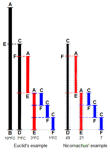
La Méthode d'Euclide pour trouver le plus grand diviseur commun (PGCD)
de deux longueurs de départ`BA` et `DC`, toutes deux définies comme étant
multiples d'une longueur commune. La longueur `DC` étant
plus courte, elle est utilisée pour « mesurer » `BA`, mais une seule fois car
le reste `EA` est inférieur à `DC`. `EA` mesure maintenant (deux fois)
la longueur la plus courte `DC`, le reste `FC` étant plus court que `EA`.
Alors `FC` mesure (trois fois) la longueur `EA`. Parce qu'il y a
pas de reste, le processus se termine par `FC` étant le « PGCD ».
À droite, l'exemple de Nicomaque de Gérase avec les nombres `49` et `21`
ayan un PGCD de `7` (dérivé de Heath 1908: 300).

Un de rectangle de dimensions `24 par 60` peux se carreler en carrés de `12 par 12`,
puisque `12` est le PGCD ed `24` et `60`. De façon générale,
un rectangle de dimension `a par b` peut se carreler en carrés
de côté `c`, seulement si `c` est un diviseur commun de `a` et `b`.

Animation basée sur la soustraction via l'algorithme euclidien.
Le rectangle initial a les dimensions `a = 1071` et `b = 462`.
Des carrés de taille `462 × 462` y sont placés en laissant un
rectangle de `462 × 147`. Ce rectangle est carrelé avec des
carrés de `147 × 147` jusqu'à ce qu'un rectangle de `21 × 147` soit laissé,
qui à son tour estcarrelé avec des carrés `21 × 21`,
ne laissant aucune zone non couverte.
La plus petite taille carrée, `21`, est le PGCD de `1071` et `462`.
## References
[Wikipedia](https://fr.wikipedia.org/wiki/Algorithme_d%27Euclide)
================================================
FILE: src/algorithms/math/euclidean-algorithm/README.md
================================================
# Euclidean algorithm
_Read this in other languages:_
[français](README.fr-FR.md).
In mathematics, the Euclidean algorithm, or Euclid's algorithm,
is an efficient method for computing the greatest common divisor
(GCD) of two numbers, the largest number that divides both of
them without leaving a remainder.
The Euclidean algorithm is based on the principle that the
greatest common divisor of two numbers does not change if
the larger number is replaced by its difference with the
smaller number. For example, `21` is the GCD of `252` and
`105` (as `252 = 21 × 12` and `105 = 21 × 5`), and the same
number `21` is also the GCD of `105` and `252 − 105 = 147`.
Since this replacement reduces the larger of the two numbers,
repeating this process gives successively smaller pairs of
numbers until the two numbers become equal.
When that occurs, they are the GCD of the original two numbers.
By reversing the steps, the GCD can be expressed as a sum of
the two original numbers each multiplied by a positive or
negative integer, e.g., `21 = 5 × 10⁵ + (−2) × 252`.
The fact that the GCD can always be expressed in this way is
known as Bézout's identity.

Euclid's method for finding the greatest common divisor (GCD)
of two starting lengths `BA` and `DC`, both defined to be
multiples of a common "unit" length. The length `DC` being
shorter, it is used to "measure" `BA`, but only once because
remainder `EA` is less than `DC`. EA now measures (twice)
the shorter length `DC`, with remainder `FC` shorter than `EA`.
Then `FC` measures (three times) length `EA`. Because there is
no remainder, the process ends with `FC` being the `GCD`.
On the right Nicomachus' example with numbers `49` and `21`
resulting in their GCD of `7` (derived from Heath 1908:300).

A `24-by-60` rectangle is covered with ten `12-by-12` square
tiles, where `12` is the GCD of `24` and `60`. More generally,
an `a-by-b` rectangle can be covered with square tiles of
side-length `c` only if `c` is a common divisor of `a` and `b`.

Subtraction-based animation of the Euclidean algorithm.
The initial rectangle has dimensions `a = 1071` and `b = 462`.
Squares of size `462×462` are placed within it leaving a
`462×147` rectangle. This rectangle is tiled with `147×147`
squares until a `21×147` rectangle is left, which in turn is
tiled with `21×21` squares, leaving no uncovered area.
The smallest square size, `21`, is the GCD of `1071` and `462`.
## References
[Wikipedia](https://en.wikipedia.org/wiki/Euclidean_algorithm)
================================================
FILE: src/algorithms/math/euclidean-algorithm/__test__/euclideanAlgorithm.test.js
================================================
import euclideanAlgorithm from '../euclideanAlgorithm';
describe('euclideanAlgorithm', () => {
it('should calculate GCD recursively', () => {
expect(euclideanAlgorithm(0, 0)).toBe(0);
expect(euclideanAlgorithm(2, 0)).toBe(2);
expect(euclideanAlgorithm(0, 2)).toBe(2);
expect(euclideanAlgorithm(1, 2)).toBe(1);
expect(euclideanAlgorithm(2, 1)).toBe(1);
expect(euclideanAlgorithm(6, 6)).toBe(6);
expect(euclideanAlgorithm(2, 4)).toBe(2);
expect(euclideanAlgorithm(4, 2)).toBe(2);
expect(euclideanAlgorithm(12, 4)).toBe(4);
expect(euclideanAlgorithm(4, 12)).toBe(4);
expect(euclideanAlgorithm(5, 13)).toBe(1);
expect(euclideanAlgorithm(27, 13)).toBe(1);
expect(euclideanAlgorithm(24, 60)).toBe(12);
expect(euclideanAlgorithm(60, 24)).toBe(12);
expect(euclideanAlgorithm(252, 105)).toBe(21);
expect(euclideanAlgorithm(105, 252)).toBe(21);
expect(euclideanAlgorithm(1071, 462)).toBe(21);
expect(euclideanAlgorithm(462, 1071)).toBe(21);
expect(euclideanAlgorithm(462, -1071)).toBe(21);
expect(euclideanAlgorithm(-462, -1071)).toBe(21);
});
});
================================================
FILE: src/algorithms/math/euclidean-algorithm/__test__/euclideanAlgorithmIterative.test.js
================================================
import euclideanAlgorithmIterative from '../euclideanAlgorithmIterative';
describe('euclideanAlgorithmIterative', () => {
it('should calculate GCD iteratively', () => {
expect(euclideanAlgorithmIterative(0, 0)).toBe(0);
expect(euclideanAlgorithmIterative(2, 0)).toBe(2);
expect(euclideanAlgorithmIterative(0, 2)).toBe(2);
expect(euclideanAlgorithmIterative(1, 2)).toBe(1);
expect(euclideanAlgorithmIterative(2, 1)).toBe(1);
expect(euclideanAlgorithmIterative(6, 6)).toBe(6);
expect(euclideanAlgorithmIterative(2, 4)).toBe(2);
expect(euclideanAlgorithmIterative(4, 2)).toBe(2);
expect(euclideanAlgorithmIterative(12, 4)).toBe(4);
expect(euclideanAlgorithmIterative(4, 12)).toBe(4);
expect(euclideanAlgorithmIterative(5, 13)).toBe(1);
expect(euclideanAlgorithmIterative(27, 13)).toBe(1);
expect(euclideanAlgorithmIterative(24, 60)).toBe(12);
expect(euclideanAlgorithmIterative(60, 24)).toBe(12);
expect(euclideanAlgorithmIterative(252, 105)).toBe(21);
expect(euclideanAlgorithmIterative(105, 252)).toBe(21);
expect(euclideanAlgorithmIterative(1071, 462)).toBe(21);
expect(euclideanAlgorithmIterative(462, 1071)).toBe(21);
expect(euclideanAlgorithmIterative(462, -1071)).toBe(21);
expect(euclideanAlgorithmIterative(-462, -1071)).toBe(21);
});
});
================================================
FILE: src/algorithms/math/euclidean-algorithm/euclideanAlgorithm.js
================================================
/**
* Recursive version of Euclidean Algorithm of finding greatest common divisor (GCD).
* @param {number} originalA
* @param {number} originalB
* @return {number}
*/
export default function euclideanAlgorithm(originalA, originalB) {
// Make input numbers positive.
const a = Math.abs(originalA);
const b = Math.abs(originalB);
// To make algorithm work faster instead of subtracting one number from the other
// we may use modulo operation.
return (b === 0) ? a : euclideanAlgorithm(b, a % b);
}
================================================
FILE: src/algorithms/math/euclidean-algorithm/euclideanAlgorithmIterative.js
================================================
/**
* Iterative version of Euclidean Algorithm of finding greatest common divisor (GCD).
* @param {number} originalA
* @param {number} originalB
* @return {number}
*/
export default function euclideanAlgorithmIterative(originalA, originalB) {
// Make input numbers positive.
let a = Math.abs(originalA);
let b = Math.abs(originalB);
// Subtract one number from another until both numbers would become the same.
// This will be out GCD. Also quit the loop if one of the numbers is zero.
while (a && b && a !== b) {
[a, b] = a > b ? [a - b, b] : [a, b - a];
}
// Return the number that is not equal to zero since the last subtraction (it will be a GCD).
return a || b;
}
================================================
FILE: src/algorithms/math/euclidean-distance/README.md
================================================
# Euclidean Distance
In mathematics, the **Euclidean distance** between two points in Euclidean space is the length of a line segment between the two points. It can be calculated from the Cartesian coordinates of the points using the Pythagorean theorem, therefore occasionally being called the Pythagorean distance.

## Distance formulas
### One dimension
The distance between any two points on the real line is the absolute value of the numerical difference of their coordinates

### Two dimensions

### Higher dimensions
In three dimensions, for points given by their Cartesian coordinates, the distance is

Example: the distance between the two points `(8,2,6)` and `(3,5,7)`:

In general, for points given by Cartesian coordinates in `n`-dimensional Euclidean space, the distance is

## References
- [Euclidean Distance on MathIsFun](https://www.mathsisfun.com/algebra/distance-2-points.html)
- [Euclidean Distance on Wikipedia](https://en.wikipedia.org/wiki/Euclidean_distance)
================================================
FILE: src/algorithms/math/euclidean-distance/__tests__/euclideanDistance.test.js
================================================
import euclideanDistance from '../euclideanDistance';
describe('euclideanDistance', () => {
it('should calculate euclidean distance between vectors', () => {
expect(euclideanDistance([[1]], [[2]])).toEqual(1);
expect(euclideanDistance([[2]], [[1]])).toEqual(1);
expect(euclideanDistance([[5, 8]], [[7, 3]])).toEqual(5.39);
expect(euclideanDistance([[5], [8]], [[7], [3]])).toEqual(5.39);
expect(euclideanDistance([[8, 2, 6]], [[3, 5, 7]])).toEqual(5.92);
expect(euclideanDistance([[8], [2], [6]], [[3], [5], [7]])).toEqual(5.92);
expect(euclideanDistance([[[8]], [[2]], [[6]]], [[[3]], [[5]], [[7]]])).toEqual(5.92);
});
it('should throw an error in case if two matrices are of different shapes', () => {
expect(() => euclideanDistance([[1]], [[[2]]])).toThrow(
'Matrices have different dimensions',
);
expect(() => euclideanDistance([[1]], [[2, 3]])).toThrow(
'Matrices have different shapes',
);
});
});
================================================
FILE: src/algorithms/math/euclidean-distance/euclideanDistance.js
================================================
/**
* @typedef {import('../matrix/Matrix.js').Matrix} Matrix
*/
import * as mtrx from '../matrix/Matrix';
/**
* Calculates the euclidean distance between 2 matrices.
*
* @param {Matrix} a
* @param {Matrix} b
* @returns {number}
* @trows {Error}
*/
const euclideanDistance = (a, b) => {
mtrx.validateSameShape(a, b);
let squaresTotal = 0;
mtrx.walk(a, (indices, aCellValue) => {
const bCellValue = mtrx.getCellAtIndex(b, indices);
squaresTotal += (aCellValue - bCellValue) ** 2;
});
return Number(Math.sqrt(squaresTotal).toFixed(2));
};
export default euclideanDistance;
================================================
FILE: src/algorithms/math/factorial/README.fr-FR.md
================================================
# Factorielle
_Lisez ceci dans d'autres langues:_
[english](README.md), [_简体中文_](README.zh-CN.md).
En mathématiques, la factorielle d'un entier naturel `n`,
notée avec un point d'exclamation `n!`, est le produit des nombres entiers
strictement positifs inférieurs ou égaux à n. Par exemple:
```
5! = 5 * 4 * 3 * 2 * 1 = 120
```
| n | n! |
| --- | ----------------: |
| 0 | 1 |
| 1 | 1 |
| 2 | 2 |
| 3 | 6 |
| 4 | 24 |
| 5 | 120 |
| 6 | 720 |
| 7 | 5 040 |
| 8 | 40 320 |
| 9 | 362 880 |
| 10 | 3 628 800 |
| 11 | 39 916 800 |
| 12 | 479 001 600 |
| 13 | 6 227 020 800 |
| 14 | 87 178 291 200 |
| 15 | 1 307 674 368 000 |
## References
[Wikipedia](https://fr.wikipedia.org/wiki/Factorielle)
================================================
FILE: src/algorithms/math/factorial/README.ka-GE.md
================================================
# ფაქტორიალი
მათემატიკაში `n` ნატურალური რიცხვის ფაქტორიალი
(აღინიშნება `n!` სიმბოლოთი)
არის ყველა ნატურალური რიცხვის ნამრავლი 1-იდან `n`-ის ჩათვლით. მაგალითად:
```
5! = 5 * 4 * 3 * 2 * 1 = 120
```
| n | n! |
| --- | ----------------: |
| 0 | 1 |
| 1 | 1 |
| 2 | 2 |
| 3 | 6 |
| 4 | 24 |
| 5 | 120 |
| 6 | 720 |
| 7 | 5 040 |
| 8 | 40 320 |
| 9 | 362 880 |
| 10 | 3 628 800 |
| 11 | 39 916 800 |
| 12 | 479 001 600 |
| 13 | 6 227 020 800 |
| 14 | 87 178 291 200 |
| 15 | 1 307 674 368 000 |
## სქოლიო
[Wikipedia](https://ka.wikipedia.org/wiki/%E1%83%9B%E1%83%90%E1%83%97%E1%83%94%E1%83%9B%E1%83%90%E1%83%A2%E1%83%98%E1%83%99%E1%83%A3%E1%83%A0%E1%83%98_%E1%83%A4%E1%83%90%E1%83%A5%E1%83%A2%E1%83%9D%E1%83%A0%E1%83%98%E1%83%90%E1%83%9A%E1%83%98)
================================================
FILE: src/algorithms/math/factorial/README.md
================================================
# Factorial
_Read this in other languages:_
[_简体中文_](README.zh-CN.md), [_Français_](README.fr-FR.md), [_Türkçe_](README.tr-TR.md), [_ქართული_](README.ka-GE.md), [_Українська_](README.uk-UA.md).
In mathematics, the factorial of a non-negative integer `n`,
denoted by `n!`, is the product of all positive integers less
than or equal to `n`. For example:
```
5! = 5 * 4 * 3 * 2 * 1 = 120
```
| n | n! |
| --- | ----------------: |
| 0 | 1 |
| 1 | 1 |
| 2 | 2 |
| 3 | 6 |
| 4 | 24 |
| 5 | 120 |
| 6 | 720 |
| 7 | 5 040 |
| 8 | 40 320 |
| 9 | 362 880 |
| 10 | 3 628 800 |
| 11 | 39 916 800 |
| 12 | 479 001 600 |
| 13 | 6 227 020 800 |
| 14 | 87 178 291 200 |
| 15 | 1 307 674 368 000 |
## References
[Wikipedia](https://en.wikipedia.org/wiki/Factorial)
================================================
FILE: src/algorithms/math/factorial/README.tr-TR.md
================================================
# Faktöriyel
_Bunu diğer dillerde okuyun:_
[_简体中文_](README.zh-CN.md), [français](README.fr-FR.md).
Faktöriyel, matematikte, sağına ünlem işareti konulmuş sayıya
verilen isim, daha genel olan Gama fonksiyonunun tam sayılarla
sınırlanmış özel bir durumudur. 1'den başlayarak belirli bir
sayma sayısına kadar olan sayıların çarpımına o sayının
faktöriyeli denir. Basit bir şekilde faktöriyel, n tane ayrık
elemanın kaç farklı şekilde sıralanabileceğidir.
```
5! = 5 * 4 * 3 * 2 * 1 = 120
```
| n | n! |
| --- | ----------------: |
| 0 | 1 |
| 1 | 1 |
| 2 | 2 |
| 3 | 6 |
| 4 | 24 |
| 5 | 120 |
| 6 | 720 |
| 7 | 5 040 |
| 8 | 40 320 |
| 9 | 362 880 |
| 10 | 3 628 800 |
| 11 | 39 916 800 |
| 12 | 479 001 600 |
| 13 | 6 227 020 800 |
| 14 | 87 178 291 200 |
| 15 | 1 307 674 368 000 |
## Referanslar
[Wikipedia](https://en.wikipedia.org/wiki/Factorial)
================================================
FILE: src/algorithms/math/factorial/README.uk-UA.md
================================================
# Факторіал
_Прочитайте це іншими мовами:_
[_English_](README.md), [_简体中文_](README.zh-CN.md), [_Français_](README.fr-FR.md), [_Türkçe_](README.tr-TR.md), [_ქართული_](README.ka-GE.md).
У математиці факторіал невід'ємного цілого числа `n`, позначений `n!`, є добутком усіх натуральних чисел, менших або рівних `n`. Наприклад:
```
5! = 5 * 4 * 3 * 2 * 1 = 120
```
| n | n! |
| --- | ----------------: |
| 0 | 1 |
| 1 | 1 |
| 2 | 2 |
| 3 | 6 |
| 4 | 24 |
| 5 | 120 |
| 6 | 720 |
| 7 | 5 040 |
| 8 | 40 320 |
| 9 | 362 880 |
| 10 | 3 628 800 |
| 11 | 39 916 800 |
| 12 | 479 001 600 |
| 13 | 6 227 020 800 |
| 14 | 87 178 291 200 |
| 15 | 1 307 674 368 000 |
## Посилання
[Wikipedia](https://uk.wikipedia.org/wiki/%D0%A4%D0%B0%D0%BA%D1%82%D0%BE%D1%80%D1%96%D0%B0%D0%BB)
================================================
FILE: src/algorithms/math/factorial/README.zh-CN.md
================================================
# 阶乘
在数学上, 一个正整数 `n` 的阶乘 (写作 `n!`), 就是所有小于等于 `n` 的正整数的乘积. 比如:
```
5! = 5 * 4 * 3 * 2 * 1 = 120
```
| n | n! |
| ----- | --------------------------: |
| 0 | 1 |
| 1 | 1 |
| 2 | 2 |
| 3 | 6 |
| 4 | 24 |
| 5 | 120 |
| 6 | 720 |
| 7 | 5 040 |
| 8 | 40 320 |
| 9 | 362 880 |
| 10 | 3 628 800 |
| 11 | 39 916 800 |
| 12 | 479 001 600 |
| 13 | 6 227 020 800 |
| 14 | 87 178 291 200 |
| 15 | 1 307 674 368 000 |
================================================
FILE: src/algorithms/math/factorial/__test__/factorial.test.js
================================================
import factorial from '../factorial';
describe('factorial', () => {
it('should calculate factorial', () => {
expect(factorial(0)).toBe(1);
expect(factorial(1)).toBe(1);
expect(factorial(5)).toBe(120);
expect(factorial(8)).toBe(40320);
expect(factorial(10)).toBe(3628800);
});
});
================================================
FILE: src/algorithms/math/factorial/__test__/factorialRecursive.test.js
================================================
import factorialRecursive from '../factorialRecursive';
describe('factorialRecursive', () => {
it('should calculate factorial', () => {
expect(factorialRecursive(0)).toBe(1);
expect(factorialRecursive(1)).toBe(1);
expect(factorialRecursive(5)).toBe(120);
expect(factorialRecursive(8)).toBe(40320);
expect(factorialRecursive(10)).toBe(3628800);
});
});
================================================
FILE: src/algorithms/math/factorial/factorial.js
================================================
/**
* @param {number} number
* @return {number}
*/
export default function factorial(number) {
let result = 1;
for (let i = 2; i <= number; i += 1) {
result *= i;
}
return result;
}
================================================
FILE: src/algorithms/math/factorial/factorialRecursive.js
================================================
/**
* @param {number} number
* @return {number}
*/
export default function factorialRecursive(number) {
return number > 1 ? number * factorialRecursive(number - 1) : 1;
}
================================================
FILE: src/algorithms/math/fast-powering/README.fr-FR.md
================================================
# Algorithme d'exponentiation rapide
_Read this in other languages:_
[english](README.md).
En algèbre, une **puissance** d'un nombre est le résultat de la multiplication répétée de ce nombre avec lui-même.
Elle est souvent notée en assortissant le nombre d'un entier, typographié en exposant, qui indique le nombre de fois qu'apparaît le nombre comme facteur dans cette multiplication.

## Implémentation « naïve »
Comment trouver `a` élevé à la puissance `b` ?
On multiplie `a` avec lui-même, `b` nombre de fois.
Ainsi, `a^b = a * a * a * ... * a` (`b` occurrences de `a`).
Cette opération aura un complexité linéaire, notée `O(n)`,
car la multiplication aura lieu exactement `n` fois.
## Algorithme d'exponentiation rapide
Peut-on faire mieux que cette implémentation naïve?
Oui, on peut réduire le nombre de puissance à un complexité de `O(log(n))`.
Cet algorithme utilise l'approche « diviser pour mieux régner »
pour calculer cette puissance.
En l'état, cet algorithme fonctionne pour deux entiers positifs `X` et `Y`.
L'idée derrière cet algorithme est basée sur l'observation suivante.
Lorsque `Y` est **pair**:
```text
X^Y = X^(Y/2) * X^(Y/2)
```
Lorsque `Y` est **impair**:
```text
X^Y = X^(Y//2) * X^(Y//2) * X
où Y//2 est le résultat de la division entière de Y par 2.
```
**Par exemple**
```text
2^4 = (2 * 2) * (2 * 2) = (2^2) * (2^2)
```
```text
2^5 = (2 * 2) * (2 * 2) * 2 = (2^2) * (2^2) * (2)
```
Ainsi, puisqu'à chaque étape on doits calculer
deux fois la même puissance `X ^ (Y / 2)`,
on peut optimiser en l'enregistrant dans une variable intermédiaire
pour éviter son calcul en double.
**Complexité en temps**
Comme à chaque itération nous réduisons la puissance de moitié,
nous appelons récursivement la fonction `log(n)` fois. Le complexité de temps de cet algorithme est donc réduite à:
```text
O(log(n))
```
## Références
- [YouTube](https://www.youtube.com/watch?v=LUWavfN9zEo&index=80&list=PLLXdhg_r2hKA7DPDsunoDZ-Z769jWn4R8&t=0s)
- [Wikipedia](https://fr.wikipedia.org/wiki/Exponentiation_rapide)
================================================
FILE: src/algorithms/math/fast-powering/README.md
================================================
# Fast Powering Algorithm
_Read this in other languages:_
[français](README.fr-FR.md).
**The power of a number** says how many times to use the number in a
multiplication.
It is written as a small number to the right and above the base number.

## Naive Algorithm Complexity
How to find `a` raised to the power `b`?
We multiply `a` to itself, `b` times. That
is, `a^b = a * a * a * ... * a` (`b` occurrences of `a`).
This operation will take `O(n)` time since we need to do multiplication operation
exactly `n` times.
## Fast Power Algorithm
Can we do better than naive algorithm does? Yes we may solve the task of
powering in `O(log(n))` time.
The algorithm uses divide and conquer approach to compute power. Currently the
algorithm work for two positive integers `X` and `Y`.
The idea behind the algorithm is based on the fact that:
For **even** `Y`:
```text
X^Y = X^(Y/2) * X^(Y/2)
```
For **odd** `Y`:
```text
X^Y = X^(Y//2) * X^(Y//2) * X
where Y//2 is result of division of Y by 2 without reminder.
```
**For example**
```text
2^4 = (2 * 2) * (2 * 2) = (2^2) * (2^2)
```
```text
2^5 = (2 * 2) * (2 * 2) * 2 = (2^2) * (2^2) * (2)
```
Now, since on each step we need to compute the same `X^(Y/2)` power twice we may optimise
it by saving it to some intermediate variable to avoid its duplicate calculation.
**Time Complexity**
Since each iteration we split the power by half then we will call function
recursively `log(n)` times. This the time complexity of the algorithm is reduced to:
```text
O(log(n))
```
## References
- [YouTube](https://www.youtube.com/watch?v=LUWavfN9zEo&index=80&list=PLLXdhg_r2hKA7DPDsunoDZ-Z769jWn4R8&t=0s)
- [Wikipedia](https://en.wikipedia.org/wiki/Exponentiation_by_squaring)
================================================
FILE: src/algorithms/math/fast-powering/__test__/fastPowering.test.js
================================================
import fastPowering from '../fastPowering';
describe('fastPowering', () => {
it('should compute power in log(n) time', () => {
expect(fastPowering(1, 1)).toBe(1);
expect(fastPowering(2, 0)).toBe(1);
expect(fastPowering(2, 2)).toBe(4);
expect(fastPowering(2, 3)).toBe(8);
expect(fastPowering(2, 4)).toBe(16);
expect(fastPowering(2, 5)).toBe(32);
expect(fastPowering(2, 6)).toBe(64);
expect(fastPowering(2, 7)).toBe(128);
expect(fastPowering(2, 8)).toBe(256);
expect(fastPowering(3, 4)).toBe(81);
expect(fastPowering(190, 2)).toBe(36100);
expect(fastPowering(11, 5)).toBe(161051);
expect(fastPowering(13, 11)).toBe(1792160394037);
expect(fastPowering(9, 16)).toBe(1853020188851841);
expect(fastPowering(16, 16)).toBe(18446744073709552000);
expect(fastPowering(7, 21)).toBe(558545864083284000);
expect(fastPowering(100, 9)).toBe(1000000000000000000);
});
});
================================================
FILE: src/algorithms/math/fast-powering/fastPowering.js
================================================
/**
* Fast Powering Algorithm.
* Recursive implementation to compute power.
*
* Complexity: log(n)
*
* @param {number} base - Number that will be raised to the power.
* @param {number} power - The power that number will be raised to.
* @return {number}
*/
export default function fastPowering(base, power) {
if (power === 0) {
// Anything that is raised to the power of zero is 1.
return 1;
}
if (power % 2 === 0) {
// If the power is even...
// we may recursively redefine the result via twice smaller powers:
// x^8 = x^4 * x^4.
const multiplier = fastPowering(base, power / 2);
return multiplier * multiplier;
}
// If the power is odd...
// we may recursively redefine the result via twice smaller powers:
// x^9 = x^4 * x^4 * x.
const multiplier = fastPowering(base, Math.floor(power / 2));
return multiplier * multiplier * base;
}
================================================
FILE: src/algorithms/math/fibonacci/README.fr-FR.md
================================================
# Nombre de Fibonacci
_Read this in other languages:_
[english](README.md),
[ქართული](README.ka-GE.md).
En mathématiques, la suite de Fibonacci est une suite d'entiers
dans laquelle chaque terme (après les deux premiers)
est la somme des deux termes qui le précèdent.
Les termes de cette suite sont appelés nombres de Fibonacci:
`0, 1, 1, 2, 3, 5, 8, 13, 21, 34, 55, 89, 144, ...`
Les carrés de Fibonacci en spirale s'ajustent ensemble pour former une spirale d'or.

La spirale de Fibonacci: approximation d'une spirale d'or créée en dessinant des arcs de cercle reliant les coins opposés de carrés dans un pavage Fibonacci[4] . Celui-ci utilise des carrés de tailles 1, 1, 2, 3, 5, 8, 13, 21, et 34.

## References
- [Wikipedia](https://fr.wikipedia.org/wiki/Suite_de_Fibonacci)
================================================
FILE: src/algorithms/math/fibonacci/README.ka-GE.md
================================================
# ფიბონაჩის რიცხვი
მათემატიკაში ფიბონაჩის მიმდევრობა წარმოადგენს მთელ რიცხვთა მიმდევრობას,
რომელშიც ყოველი რიცხვი (პირველი ორი რიცხვის შემდეგ)
მისი წინამორბედი ორი რიცხვის
ჯამის ტოლია:
`0, 1, 1, 2, 3, 5, 8, 13, 21, 34, 55, 89, 144, ...`
კვადრატების წყობა, სადაც ყოველი კვადრატის გვერდების სიგრძე, თანმიმდევრობით, ფიბონაჩის რიცხვებს შეესაბამება

ფიბონაჩის სპირალი: ოქროს სპირალის აპროქსიმაცია, რომელიც შექმნილია კვადრატების მოპირდაპირე კუთხეებს შორის შემაერთებელი რკალების გავლებით;[4] ამ შემთხვევაში, გამოყენებულ კვადრატთა [გვერდების] ზომებია: 1, 1, 2, 3, 5, 8, 13 და 21.

## სქოლიო
- [Wikipedia](https://en.wikipedia.org/wiki/Fibonacci_number)
================================================
FILE: src/algorithms/math/fibonacci/README.md
================================================
# Fibonacci Number
_Read this in other languages:_
[français](README.fr-FR.md),
[简体中文](README.zh-CN.md),
[ქართული](README.ka-GE.md).
In mathematics, the Fibonacci numbers are the numbers in the following
integer sequence, called the Fibonacci sequence, and characterized by
the fact that every number after the first two is the sum of the two
preceding ones:
`0, 1, 1, 2, 3, 5, 8, 13, 21, 34, 55, 89, 144, ...`
A tiling with squares whose side lengths are successive Fibonacci numbers

The Fibonacci spiral: an approximation of the golden spiral created by drawing circular arcs connecting the opposite corners of squares in the Fibonacci tiling;[4] this one uses squares of sizes 1, 1, 2, 3, 5, 8, 13 and 21.

## References
- [Wikipedia](https://en.wikipedia.org/wiki/Fibonacci_number)
================================================
FILE: src/algorithms/math/fibonacci/README.zh-CN.md
================================================
# 斐波那契数
_Read this in other languages:_
[français](README.fr-FR.md),
[english](README.md),
[ქართული](README.ka-GE.md).
在数学中,斐波那契数是以下整数序列(称为斐波那契数列)中的数字,其特征在于前两个数字之后的每个数字都是前两个数字的和:
`0, 1, 1, 2, 3, 5, 8, 13, 21, 34, 55, 89, 144, ...`
边长为连续斐波纳契数的正方形平铺

斐波那契螺旋:通过绘制连接斐波那契平铺中正方形的相对角的圆弧而创建的金色螺旋的近似值; [4]该三角形使用大小为1、1、2、3、5、8、13和21的正方形。

## References
- [Wikipedia](https://en.wikipedia.org/wiki/Fibonacci_number)
================================================
FILE: src/algorithms/math/fibonacci/__test__/fibonacci.test.js
================================================
import fibonacci from '../fibonacci';
describe('fibonacci', () => {
it('should calculate fibonacci correctly', () => {
expect(fibonacci(1)).toEqual([1]);
expect(fibonacci(2)).toEqual([1, 1]);
expect(fibonacci(3)).toEqual([1, 1, 2]);
expect(fibonacci(4)).toEqual([1, 1, 2, 3]);
expect(fibonacci(5)).toEqual([1, 1, 2, 3, 5]);
expect(fibonacci(6)).toEqual([1, 1, 2, 3, 5, 8]);
expect(fibonacci(7)).toEqual([1, 1, 2, 3, 5, 8, 13]);
expect(fibonacci(8)).toEqual([1, 1, 2, 3, 5, 8, 13, 21]);
expect(fibonacci(9)).toEqual([1, 1, 2, 3, 5, 8, 13, 21, 34]);
expect(fibonacci(10)).toEqual([1, 1, 2, 3, 5, 8, 13, 21, 34, 55]);
});
});
================================================
FILE: src/algorithms/math/fibonacci/__test__/fibonacciNth.test.js
================================================
import fibonacciNth from '../fibonacciNth';
describe('fibonacciNth', () => {
it('should calculate fibonacci correctly', () => {
expect(fibonacciNth(1)).toBe(1);
expect(fibonacciNth(2)).toBe(1);
expect(fibonacciNth(3)).toBe(2);
expect(fibonacciNth(4)).toBe(3);
expect(fibonacciNth(5)).toBe(5);
expect(fibonacciNth(6)).toBe(8);
expect(fibonacciNth(7)).toBe(13);
expect(fibonacciNth(8)).toBe(21);
expect(fibonacciNth(20)).toBe(6765);
expect(fibonacciNth(30)).toBe(832040);
expect(fibonacciNth(50)).toBe(12586269025);
expect(fibonacciNth(70)).toBe(190392490709135);
expect(fibonacciNth(71)).toBe(308061521170129);
expect(fibonacciNth(72)).toBe(498454011879264);
expect(fibonacciNth(73)).toBe(806515533049393);
expect(fibonacciNth(74)).toBe(1304969544928657);
expect(fibonacciNth(75)).toBe(2111485077978050);
});
});
================================================
FILE: src/algorithms/math/fibonacci/__test__/fibonacciNthClosedForm.test.js
================================================
import fibonacciNthClosedForm from '../fibonacciNthClosedForm';
describe('fibonacciClosedForm', () => {
it('should throw an error when trying to calculate fibonacci for not allowed positions', () => {
const calculateFibonacciForNotAllowedPosition = () => {
fibonacciNthClosedForm(76);
};
expect(calculateFibonacciForNotAllowedPosition).toThrow();
});
it('should calculate fibonacci correctly', () => {
expect(fibonacciNthClosedForm(1)).toBe(1);
expect(fibonacciNthClosedForm(2)).toBe(1);
expect(fibonacciNthClosedForm(3)).toBe(2);
expect(fibonacciNthClosedForm(4)).toBe(3);
expect(fibonacciNthClosedForm(5)).toBe(5);
expect(fibonacciNthClosedForm(6)).toBe(8);
expect(fibonacciNthClosedForm(7)).toBe(13);
expect(fibonacciNthClosedForm(8)).toBe(21);
expect(fibonacciNthClosedForm(20)).toBe(6765);
expect(fibonacciNthClosedForm(30)).toBe(832040);
expect(fibonacciNthClosedForm(50)).toBe(12586269025);
expect(fibonacciNthClosedForm(70)).toBe(190392490709135);
});
});
================================================
FILE: src/algorithms/math/fibonacci/fibonacci.js
================================================
/**
* Return a fibonacci sequence as an array.
*
* @param n
* @return {number[]}
*/
export default function fibonacci(n) {
const fibSequence = [1];
let currentValue = 1;
let previousValue = 0;
if (n === 1) {
return fibSequence;
}
let iterationsCounter = n - 1;
while (iterationsCounter) {
currentValue += previousValue;
previousValue = currentValue - previousValue;
fibSequence.push(currentValue);
iterationsCounter -= 1;
}
return fibSequence;
}
================================================
FILE: src/algorithms/math/fibonacci/fibonacciNth.js
================================================
/**
* Calculate fibonacci number at specific position using Dynamic Programming approach.
*
* @param n
* @return {number}
*/
export default function fibonacciNth(n) {
let currentValue = 1;
let previousValue = 0;
if (n === 1) {
return 1;
}
let iterationsCounter = n - 1;
while (iterationsCounter) {
currentValue += previousValue;
previousValue = currentValue - previousValue;
iterationsCounter -= 1;
}
return currentValue;
}
================================================
FILE: src/algorithms/math/fibonacci/fibonacciNthClosedForm.js
================================================
/**
* Calculate fibonacci number at specific position using closed form function (Binet's formula).
* @see: https://en.wikipedia.org/wiki/Fibonacci_number#Closed-form_expression
*
* @param {number} position - Position number of fibonacci sequence (must be number from 1 to 75).
* @return {number}
*/
export default function fibonacciClosedForm(position) {
const topMaxValidPosition = 70;
// Check that position is valid.
if (position < 1 || position > topMaxValidPosition) {
throw new Error(`Can't handle position smaller than 1 or greater than ${topMaxValidPosition}`);
}
// Calculate √5 to re-use it in further formulas.
const sqrt5 = Math.sqrt(5);
// Calculate φ constant (≈ 1.61803).
const phi = (1 + sqrt5) / 2;
// Calculate fibonacci number using Binet's formula.
return Math.floor((phi ** position) / sqrt5 + 0.5);
}
================================================
FILE: src/algorithms/math/fourier-transform/README.fr-FR.md
================================================
# Transformation de Fourier
_Read this in other languages:_
[english](README.md).
## Définitions
La transformation de Fourier (**ℱ**) est une opération qui transforme
une fonction intégrable sur ℝ en une autre fonction,
décrivant le spectre fréquentiel de cette dernière
La **Transformée de Fourier Discrète** (**TFD**) convertit une séquence finie d'échantillons également espacés d'une fonction, dans une séquence de même longueur d'échantillons, également espacés de la Transformée de Fourier à temps discret (TFtd), qui est une fonction complexe de la fréquence.
L'intervalle auquel le TFtd est échantillonné est l'inverse de la durée de la séquence d'entrée.
Une TFD inverse est une série de Fourier, utilisant les échantillons TFtd comme coefficients de sinusoïdes complexes aux fréquences TFtd correspondantes. Elle a les mêmes valeurs d'échantillonnage que la
séquence d'entrée originale. On dit donc que la TFD est une représentation du domaine fréquentiel
de la séquence d'entrée d'origine. Si la séquence d'origine couvre toutes les
valeurs non nulles d'une fonction, sa TFtd est continue (et périodique), et la TFD fournit
les échantillons discrets d'une fenêtre. Si la séquence d'origine est un cycle d'une fonction périodique, la TFD fournit toutes les valeurs non nulles d'une fenêtre TFtd.
Transformée de Fourier Discrète converti une séquence de `N` nombres complexes:
{xn} = x0, x1, x2 ..., xN-1
en une atre séquence de nombres complexes::
{Xk} = X0, X1, X2 ..., XN-1
décrite par:

The **Transformée de Fourier à temps discret** (**TFtd**) est une forme d'analyse de Fourier
qui s'applique aux échantillons uniformément espacés d'une fonction continue. Le terme "temps discret" fait référence au fait que la transformée fonctionne sur des données discrètes
(échantillons) dont l'intervalle a souvent des unités de temps.
À partir des seuls échantillons, elle produit une fonction de fréquence qui est une somme périodique de la
Transformée de Fourier continue de la fonction continue d'origine.
A **Transformation de Fourier rapide** (**FFT** pour Fast Fourier Transform) est un algorithme de calcul de la transformation de Fourier discrète (TFD). Il est couramment utilisé en traitement numérique du signal pour transformer des données discrètes du domaine temporel dans le domaine fréquentiel, en particulier dans les oscilloscopes numériques (les analyseurs de spectre utilisant plutôt des filtres analogiques, plus précis). Son efficacité permet de réaliser des filtrages en modifiant le spectre et en utilisant la transformation inverse (filtre à réponse impulsionnelle finie).
Cette transformation peut être illustée par la formule suivante. Sur la période de temps mesurée
dans le diagramme, le signal contient 3 fréquences dominantes distinctes.
Vue d'un signal dans le domaine temporel et fréquentiel:
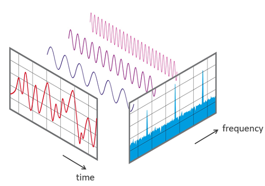
An FFT algorithm computes the discrete Fourier transform (DFT) of a sequence, or
its inverse (IFFT). Fourier analysis converts a signal from its original domain
to a representation in the frequency domain and vice versa. An FFT rapidly
computes such transformations by factorizing the DFT matrix into a product of
sparse (mostly zero) factors. As a result, it manages to reduce the complexity of
computing the DFT from O(n2), which arises if one simply applies the
definition of DFT, to O(n log n), where n is the data size.
Un algorithme FFT calcule la Transformée de Fourier discrète (TFD) d'une séquence, ou
son inverse (IFFT). L'analyse de Fourier convertit un signal de son domaine d'origine
en une représentation dans le domaine fréquentiel et vice versa. Une FFT
calcule rapidement ces transformations en factorisant la matrice TFD en un produit de
facteurs dispersés (généralement nuls). En conséquence, il parvient à réduire la complexité de
calcul de la TFD de O (n 2 ), qui survient si l'on applique simplement la
définition de TFD, à O (n log n), où n est la taille des données.
Voici une analyse de Fourier discrète d'une somme d'ondes cosinus à 10, 20, 30, 40,
et 50 Hz:
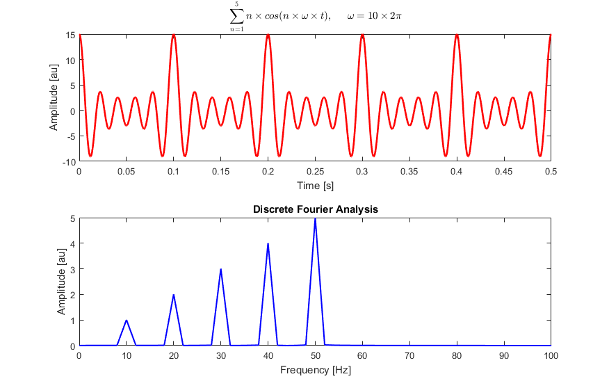
## Explanation
La Transformée de Fourier est l'une des connaissances les plus importante jamais découverte. Malheureusement, le
son sens est enfoui dans des équations denses::
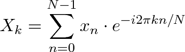
et
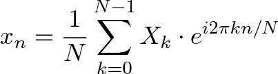
Plutôt que se noyer dans les symboles, faisons en premier lieu l'expérience de l'idée principale. Voici une métaphore en français simple:
- _Que fait la transformée de Fourier ?_ A partir d'un smoothie, elle trouve sa recette.
- _Comment ?_ Elle passe le smoothie dans un filtre pour en extraire chaque ingrédient.
- _Pourquoi ?_ Les recettes sont plus faciles à analyser, comparer et modifier que le smoothie lui-même.
- _Comment récupérer le smoothie ?_ Re-mélanger les ingrédients.
**Pensez en cercles, pas seulement en sinusoïdes**
La transformée de Fourier concerne des trajectoires circulaires (pas les sinusoïdes 1-d)
et la formuled'Euler est une manière intelligente d'en générer une:
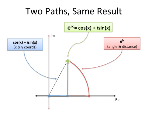
Doit-on utiliser des exposants imaginaires pour se déplacer en cercle ? Non. Mais c'est pratique
et compact. Et bien sûr, nous pouvons décrire notre chemin comme un mouvement coordonné en deux
dimensions (réelle et imaginaire), mais n'oubliez pas la vue d'ensemble: nous sommes juste
en déplacement dans un cercle.
**À la découverte de la transformation complète**
L'idée générale: notre signal n'est qu'un tas de pics de temps, d'instant T ! Si nous combinons les
recettes pour chaque pic de temps, nous devrions obtenir la recette du signal complet.
La transformée de Fourier construit cette recette fréquence par fréquence:
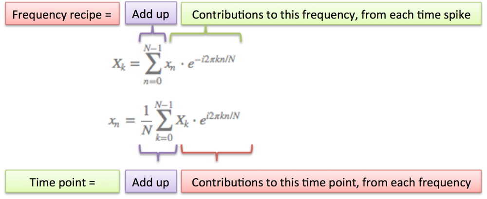
Quelques notes
- N = nombre d'échantillons de temps dont nous disposons
- n = échantillon actuellement étudié (0 ... N-1)
- xn = valeur du signal au temps n
- k = fréquence actuellement étudiée (0 Hertz up to N-1 Hertz)
- Xk = quantité de fréquence k dans le signal (amplitude et phase, un nombre complexe)
- Le facteur 1 / N est généralement déplacé vers la transformée inverse (passant des fréquences au temps). Ceci est autorisé, bien que je préfère 1 / N dans la transformation directe car cela donne les tailles réelles des pics de temps. Vous pouvez être plus ambitieux et utiliser 1 / racine carrée de (N) sur les deux transformations (aller en avant et en arrière crée le facteur 1 / N).
- n/N est le pourcentage du temps que nous avons passé. 2 _ pi _ k est notre vitesse en radians/s. e ^ -ix est notre chemin circulaire vers l'arrière. La combinaison est la distance parcourue, pour cette vitesse et ce temps.
- Les équations brutes de la transformée de Fourier consiste simplement à "ajouter les nombres complexes". De nombreux langages de programmation ne peuvent pas gérer directement les nombres complexes, on converti donc tout en coordonnées rectangulaires, pour les ajouter.
Stuart Riffle a une excellente interprétation de la transformée de Fourier:
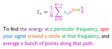
## Références
- Wikipedia
- [TF](https://fr.wikipedia.org/wiki/Transformation_de_Fourier)
- [TFD](https://fr.wikipedia.org/wiki/Transformation_de_Fourier_discr%C3%A8te)
- [FFT](https://fr.wikipedia.org/wiki/Transformation_de_Fourier_rapide)
- [TFtd (en anglais)](https://en.wikipedia.org/wiki/Discrete-time_Fourier_transform)
- en Anglais
- [An Interactive Guide To The Fourier Transform](https://betterexplained.com/articles/an-interactive-guide-to-the-fourier-transform/)
- [DFT on YouTube by Better Explained](https://www.youtube.com/watch?v=iN0VG9N2q0U&t=0s&index=77&list=PLLXdhg_r2hKA7DPDsunoDZ-Z769jWn4R8)
- [FT on YouTube by 3Blue1Brown](https://www.youtube.com/watch?v=spUNpyF58BY&t=0s&index=76&list=PLLXdhg_r2hKA7DPDsunoDZ-Z769jWn4R8)
- [FFT on YouTube by Simon Xu](https://www.youtube.com/watch?v=htCj9exbGo0&index=78&list=PLLXdhg_r2hKA7DPDsunoDZ-Z769jWn4R8&t=0s)
================================================
FILE: src/algorithms/math/fourier-transform/README.md
================================================
# Fourier Transform
_Read this in other languages:_
[français](README.fr-FR.md).
## Definitions
The **Fourier Transform** (**FT**) decomposes a function of time (a signal) into
the frequencies that make it up, in a way similar to how a musical chord can be
expressed as the frequencies (or pitches) of its constituent notes.
The **Discrete Fourier Transform** (**DFT**) converts a finite sequence of
equally-spaced samples of a function into a same-length sequence of
equally-spaced samples of the discrete-time Fourier transform (DTFT), which is a
complex-valued function of frequency. The interval at which the DTFT is sampled
is the reciprocal of the duration of the input sequence. An inverse DFT is a
Fourier series, using the DTFT samples as coefficients of complex sinusoids at
the corresponding DTFT frequencies. It has the same sample-values as the original
input sequence. The DFT is therefore said to be a frequency domain representation
of the original input sequence. If the original sequence spans all the non-zero
values of a function, its DTFT is continuous (and periodic), and the DFT provides
discrete samples of one cycle. If the original sequence is one cycle of a periodic
function, the DFT provides all the non-zero values of one DTFT cycle.
The Discrete Fourier transform transforms a sequence of `N` complex numbers:
{xn} = x0, x1, x2 ..., xN-1
into another sequence of complex numbers:
{Xk} = X0, X1, X2 ..., XN-1
which is defined by:

The **Discrete-Time Fourier Transform** (**DTFT**) is a form of Fourier analysis
that is applicable to the uniformly-spaced samples of a continuous function. The
term discrete-time refers to the fact that the transform operates on discrete data
(samples) whose interval often has units of time. From only the samples, it
produces a function of frequency that is a periodic summation of the continuous
Fourier transform of the original continuous function.
A **Fast Fourier Transform** (**FFT**) is an algorithm that samples a signal over
a period of time (or space) and divides it into its frequency components. These
components are single sinusoidal oscillations at distinct frequencies each with
their own amplitude and phase.
This transformation is illustrated in Diagram below. Over the time period measured
in the diagram, the signal contains 3 distinct dominant frequencies.
View of a signal in the time and frequency domain:

An FFT algorithm computes the discrete Fourier transform (DFT) of a sequence, or
its inverse (IFFT). Fourier analysis converts a signal from its original domain
to a representation in the frequency domain and vice versa. An FFT rapidly
computes such transformations by factorizing the DFT matrix into a product of
sparse (mostly zero) factors. As a result, it manages to reduce the complexity of
computing the DFT from O(n2), which arises if one simply applies the
definition of DFT, to O(n log n), where n is the data size.
Here a discrete Fourier analysis of a sum of cosine waves at 10, 20, 30, 40,
and 50 Hz:

## Explanation
The Fourier Transform is one of deepest insights ever made. Unfortunately, the
meaning is buried within dense equations:

and

Rather than jumping into the symbols, let's experience the key idea firsthand. Here's a plain-English metaphor:
- _What does the Fourier Transform do?_ Given a smoothie, it finds the recipe.
- _How?_ Run the smoothie through filters to extract each ingredient.
- _Why?_ Recipes are easier to analyze, compare, and modify than the smoothie itself.
- _How do we get the smoothie back?_ Blend the ingredients.
**Think With Circles, Not Just Sinusoids**
The Fourier Transform is about circular paths (not 1-d sinusoids) and Euler's
formula is a clever way to generate one:

Must we use imaginary exponents to move in a circle? Nope. But it's convenient
and compact. And sure, we can describe our path as coordinated motion in two
dimensions (real and imaginary), but don't forget the big picture: we're just
moving in a circle.
**Discovering The Full Transform**
The big insight: our signal is just a bunch of time spikes! If we merge the
recipes for each time spike, we should get the recipe for the full signal.
The Fourier Transform builds the recipe frequency-by-frequency:

A few notes:
- N = number of time samples we have
- n = current sample we're considering (0 ... N-1)
- xn = value of the signal at time n
- k = current frequency we're considering (0 Hertz up to N-1 Hertz)
- Xk = amount of frequency k in the signal (amplitude and phase, a complex number)
- The 1/N factor is usually moved to the reverse transform (going from frequencies back to time). This is allowed, though I prefer 1/N in the forward transform since it gives the actual sizes for the time spikes. You can get wild and even use 1/sqrt(N) on both transforms (going forward and back creates the 1/N factor).
- n/N is the percent of the time we've gone through. 2 _ pi _ k is our speed in radians / sec. e^-ix is our backwards-moving circular path. The combination is how far we've moved, for this speed and time.
- The raw equations for the Fourier Transform just say "add the complex numbers". Many programming languages cannot handle complex numbers directly, so you convert everything to rectangular coordinates and add those.
Stuart Riffle has a great interpretation of the Fourier Transform:

## References
- [An Interactive Guide To The Fourier Transform](https://betterexplained.com/articles/an-interactive-guide-to-the-fourier-transform/)
- [DFT on YouTube by Better Explained](https://www.youtube.com/watch?v=iN0VG9N2q0U&t=0s&index=77&list=PLLXdhg_r2hKA7DPDsunoDZ-Z769jWn4R8)
- [FT on YouTube by 3Blue1Brown](https://www.youtube.com/watch?v=spUNpyF58BY&t=0s&index=76&list=PLLXdhg_r2hKA7DPDsunoDZ-Z769jWn4R8)
- [FFT on YouTube by Simon Xu](https://www.youtube.com/watch?v=htCj9exbGo0&index=78&list=PLLXdhg_r2hKA7DPDsunoDZ-Z769jWn4R8&t=0s)
- Wikipedia
- [FT](https://en.wikipedia.org/wiki/Fourier_transform)
- [DFT](https://www.wikiwand.com/en/Discrete_Fourier_transform)
- [DTFT](https://en.wikipedia.org/wiki/Discrete-time_Fourier_transform)
- [FFT](https://www.wikiwand.com/en/Fast_Fourier_transform)
================================================
FILE: src/algorithms/math/fourier-transform/__test__/FourierTester.js
================================================
import ComplexNumber from '../../complex-number/ComplexNumber';
export const fourierTestCases = [
{
input: [
{ amplitude: 1 },
],
output: [
{
frequency: 0, amplitude: 1, phase: 0, re: 1, im: 0,
},
],
},
{
input: [
{ amplitude: 1 },
{ amplitude: 0 },
],
output: [
{
frequency: 0, amplitude: 0.5, phase: 0, re: 0.5, im: 0,
},
{
frequency: 1, amplitude: 0.5, phase: 0, re: 0.5, im: 0,
},
],
},
{
input: [
{ amplitude: 2 },
{ amplitude: 0 },
],
output: [
{
frequency: 0, amplitude: 1, phase: 0, re: 1, im: 0,
},
{
frequency: 1, amplitude: 1, phase: 0, re: 1, im: 0,
},
],
},
{
input: [
{ amplitude: 1 },
{ amplitude: 0 },
{ amplitude: 0 },
],
output: [
{
frequency: 0, amplitude: 0.33333, phase: 0, re: 0.33333, im: 0,
},
{
frequency: 1, amplitude: 0.33333, phase: 0, re: 0.33333, im: 0,
},
{
frequency: 2, amplitude: 0.33333, phase: 0, re: 0.33333, im: 0,
},
],
},
{
input: [
{ amplitude: 1 },
{ amplitude: 0 },
{ amplitude: 0 },
{ amplitude: 0 },
],
output: [
{
frequency: 0, amplitude: 0.25, phase: 0, re: 0.25, im: 0,
},
{
frequency: 1, amplitude: 0.25, phase: 0, re: 0.25, im: 0,
},
{
frequency: 2, amplitude: 0.25, phase: 0, re: 0.25, im: 0,
},
{
frequency: 3, amplitude: 0.25, phase: 0, re: 0.25, im: 0,
},
],
},
{
input: [
{ amplitude: 0 },
{ amplitude: 1 },
{ amplitude: 0 },
{ amplitude: 0 },
],
output: [
{
frequency: 0, amplitude: 0.25, phase: 0, re: 0.25, im: 0,
},
{
frequency: 1, amplitude: 0.25, phase: -90, re: 0, im: -0.25,
},
{
frequency: 2, amplitude: 0.25, phase: 180, re: -0.25, im: 0,
},
{
frequency: 3, amplitude: 0.25, phase: 90, re: 0, im: 0.25,
},
],
},
{
input: [
{ amplitude: 0 },
{ amplitude: 0 },
{ amplitude: 1 },
{ amplitude: 0 },
],
output: [
{
frequency: 0, amplitude: 0.25, phase: 0, re: 0.25, im: 0,
},
{
frequency: 1, amplitude: 0.25, phase: 180, re: -0.25, im: 0,
},
{
frequency: 2, amplitude: 0.25, phase: 0, re: 0.25, im: 0,
},
{
frequency: 3, amplitude: 0.25, phase: 180, re: -0.25, im: 0,
},
],
},
{
input: [
{ amplitude: 0 },
{ amplitude: 0 },
{ amplitude: 0 },
{ amplitude: 2 },
],
output: [
{
frequency: 0, amplitude: 0.5, phase: 0, re: 0.5, im: 0,
},
{
frequency: 1, amplitude: 0.5, phase: 90, re: 0, im: 0.5,
},
{
frequency: 2, amplitude: 0.5, phase: 180, re: -0.5, im: 0,
},
{
frequency: 3, amplitude: 0.5, phase: -90, re: 0, im: -0.5,
},
],
},
{
input: [
{ amplitude: 0 },
{ amplitude: 1 },
{ amplitude: 0 },
{ amplitude: 2 },
],
output: [
{
frequency: 0, amplitude: 0.75, phase: 0, re: 0.75, im: 0,
},
{
frequency: 1, amplitude: 0.25, phase: 90, re: 0, im: 0.25,
},
{
frequency: 2, amplitude: 0.75, phase: 180, re: -0.75, im: 0,
},
{
frequency: 3, amplitude: 0.25, phase: -90, re: 0, im: -0.25,
},
],
},
{
input: [
{ amplitude: 4 },
{ amplitude: 1 },
{ amplitude: 0 },
{ amplitude: 2 },
],
output: [
{
frequency: 0, amplitude: 1.75, phase: 0, re: 1.75, im: 0,
},
{
frequency: 1, amplitude: 1.03077, phase: 14.03624, re: 0.99999, im: 0.25,
},
{
frequency: 2, amplitude: 0.25, phase: 0, re: 0.25, im: 0,
},
{
frequency: 3, amplitude: 1.03077, phase: -14.03624, re: 1, im: -0.25,
},
],
},
{
input: [
{ amplitude: 4 },
{ amplitude: 1 },
{ amplitude: -3 },
{ amplitude: 2 },
],
output: [
{
frequency: 0, amplitude: 1, phase: 0, re: 1, im: 0,
},
{
frequency: 1, amplitude: 1.76776, phase: 8.13010, re: 1.75, im: 0.25,
},
{
frequency: 2, amplitude: 0.5, phase: 180, re: -0.5, im: 0,
},
{
frequency: 3, amplitude: 1.76776, phase: -8.13010, re: 1.75, im: -0.24999,
},
],
},
{
input: [
{ amplitude: 1 },
{ amplitude: 2 },
{ amplitude: 3 },
{ amplitude: 4 },
],
output: [
{
frequency: 0, amplitude: 2.5, phase: 0, re: 2.5, im: 0,
},
{
frequency: 1, amplitude: 0.70710, phase: 135, re: -0.5, im: 0.49999,
},
{
frequency: 2, amplitude: 0.5, phase: 180, re: -0.5, im: 0,
},
{
frequency: 3, amplitude: 0.70710, phase: -134.99999, re: -0.49999, im: -0.5,
},
],
},
];
export default class FourierTester {
/**
* @param {function} fourierTransform
*/
static testDirectFourierTransform(fourierTransform) {
fourierTestCases.forEach((testCase) => {
const { input, output: expectedOutput } = testCase;
// Try to split input signal into sequence of pure sinusoids.
const formattedInput = input.map((sample) => sample.amplitude);
const currentOutput = fourierTransform(formattedInput);
// Check the signal has been split into proper amount of sub-signals.
expect(currentOutput.length).toBeGreaterThanOrEqual(formattedInput.length);
// Now go through all the signals and check their frequency, amplitude and phase.
expectedOutput.forEach((expectedSignal, frequency) => {
// Get template data we want to test against.
const currentSignal = currentOutput[frequency];
const currentPolarSignal = currentSignal.getPolarForm(false);
// Check all signal parameters.
expect(frequency).toBe(expectedSignal.frequency);
expect(currentSignal.re).toBeCloseTo(expectedSignal.re, 4);
expect(currentSignal.im).toBeCloseTo(expectedSignal.im, 4);
expect(currentPolarSignal.phase).toBeCloseTo(expectedSignal.phase, 4);
expect(currentPolarSignal.radius).toBeCloseTo(expectedSignal.amplitude, 4);
});
});
}
/**
* @param {function} inverseFourierTransform
*/
static testInverseFourierTransform(inverseFourierTransform) {
fourierTestCases.forEach((testCase) => {
const { input: expectedOutput, output: inputFrequencies } = testCase;
// Try to join frequencies into time signal.
const formattedInput = inputFrequencies.map((frequency) => {
return new ComplexNumber({ re: frequency.re, im: frequency.im });
});
const currentOutput = inverseFourierTransform(formattedInput);
// Check the signal has been combined of proper amount of time samples.
expect(currentOutput.length).toBeLessThanOrEqual(formattedInput.length);
// Now go through all the amplitudes and check their values.
expectedOutput.forEach((expectedAmplitudes, timer) => {
// Get template data we want to test against.
const currentAmplitude = currentOutput[timer];
// Check if current amplitude is close enough to the calculated one.
expect(currentAmplitude).toBeCloseTo(expectedAmplitudes.amplitude, 4);
});
});
}
}
================================================
FILE: src/algorithms/math/fourier-transform/__test__/discreteFourierTransform.test.js
================================================
import discreteFourierTransform from '../discreteFourierTransform';
import FourierTester from './FourierTester';
describe('discreteFourierTransform', () => {
it('should split signal into frequencies', () => {
FourierTester.testDirectFourierTransform(discreteFourierTransform);
});
});
================================================
FILE: src/algorithms/math/fourier-transform/__test__/fastFourierTransform.test.js
================================================
import fastFourierTransform from '../fastFourierTransform';
import ComplexNumber from '../../complex-number/ComplexNumber';
/**
* @param {ComplexNumber[]} sequence1
* @param {ComplexNumber[]} sequence2
* @param {Number} delta
* @return {boolean}
*/
function sequencesApproximatelyEqual(sequence1, sequence2, delta) {
if (sequence1.length !== sequence2.length) {
return false;
}
for (let numberIndex = 0; numberIndex < sequence1.length; numberIndex += 1) {
if (Math.abs(sequence1[numberIndex].re - sequence2[numberIndex].re) > delta) {
return false;
}
if (Math.abs(sequence1[numberIndex].im - sequence2[numberIndex].im) > delta) {
return false;
}
}
return true;
}
const delta = 1e-6;
describe('fastFourierTransform', () => {
it('should calculate the radix-2 discrete fourier transform #1', () => {
const input = [new ComplexNumber({ re: 0, im: 0 })];
const expectedOutput = [new ComplexNumber({ re: 0, im: 0 })];
const output = fastFourierTransform(input);
const invertedOutput = fastFourierTransform(output, true);
expect(sequencesApproximatelyEqual(expectedOutput, output, delta)).toBe(true);
expect(sequencesApproximatelyEqual(input, invertedOutput, delta)).toBe(true);
});
it('should calculate the radix-2 discrete fourier transform #2', () => {
const input = [
new ComplexNumber({ re: 1, im: 2 }),
new ComplexNumber({ re: 2, im: 3 }),
new ComplexNumber({ re: 8, im: 4 }),
];
const expectedOutput = [
new ComplexNumber({ re: 11, im: 9 }),
new ComplexNumber({ re: -10, im: 0 }),
new ComplexNumber({ re: 7, im: 3 }),
new ComplexNumber({ re: -4, im: -4 }),
];
const output = fastFourierTransform(input);
const invertedOutput = fastFourierTransform(output, true);
expect(sequencesApproximatelyEqual(expectedOutput, output, delta)).toBe(true);
expect(sequencesApproximatelyEqual(input, invertedOutput, delta)).toBe(true);
});
it('should calculate the radix-2 discrete fourier transform #3', () => {
const input = [
new ComplexNumber({ re: -83656.9359385182, im: 98724.08038374918 }),
new ComplexNumber({ re: -47537.415125808424, im: 88441.58381765135 }),
new ComplexNumber({ re: -24849.657029355192, im: -72621.79007878687 }),
new ComplexNumber({ re: 31451.27290052717, im: -21113.301128347346 }),
new ComplexNumber({ re: 13973.90836288876, im: -73378.36721594246 }),
new ComplexNumber({ re: 14981.520420492234, im: 63279.524958963884 }),
new ComplexNumber({ re: -9892.575367044381, im: -81748.44671677813 }),
new ComplexNumber({ re: -35933.00356823792, im: -46153.47157161784 }),
new ComplexNumber({ re: -22425.008561855735, im: -86284.24507370662 }),
new ComplexNumber({ re: -39327.43830818355, im: 30611.949874562706 }),
];
const expectedOutput = [
new ComplexNumber({ re: -203215.3322151, im: -100242.4827503 }),
new ComplexNumber({ re: 99217.0805705, im: 270646.9331932 }),
new ComplexNumber({ re: -305990.9040412, im: 68224.8435751 }),
new ComplexNumber({ re: -14135.7758282, im: 199223.9878095 }),
new ComplexNumber({ re: -306965.6350922, im: 26030.1025439 }),
new ComplexNumber({ re: -76477.6755206, im: 40781.9078990 }),
new ComplexNumber({ re: -48409.3099088, im: 54674.7959662 }),
new ComplexNumber({ re: -329683.0131713, im: 164287.7995937 }),
new ComplexNumber({ re: -50485.2048527, im: -330375.0546527 }),
new ComplexNumber({ re: 122235.7738708, im: 91091.6398019 }),
new ComplexNumber({ re: 47625.8850387, im: 73497.3981523 }),
new ComplexNumber({ re: -15619.8231136, im: 80804.8685410 }),
new ComplexNumber({ re: 192234.0276101, im: 160833.3072355 }),
new ComplexNumber({ re: -96389.4195635, im: 393408.4543872 }),
new ComplexNumber({ re: -173449.0825417, im: 146875.7724104 }),
new ComplexNumber({ re: -179002.5662573, im: 239821.0124341 }),
];
const output = fastFourierTransform(input);
const invertedOutput = fastFourierTransform(output, true);
expect(sequencesApproximatelyEqual(expectedOutput, output, delta)).toBe(true);
expect(sequencesApproximatelyEqual(input, invertedOutput, delta)).toBe(true);
});
});
================================================
FILE: src/algorithms/math/fourier-transform/__test__/inverseDiscreteFourierTransform.test.js
================================================
import inverseDiscreteFourierTransform from '../inverseDiscreteFourierTransform';
import FourierTester from './FourierTester';
describe('inverseDiscreteFourierTransform', () => {
it('should calculate output signal out of input frequencies', () => {
FourierTester.testInverseFourierTransform(inverseDiscreteFourierTransform);
});
});
================================================
FILE: src/algorithms/math/fourier-transform/discreteFourierTransform.js
================================================
import ComplexNumber from '../complex-number/ComplexNumber';
const CLOSE_TO_ZERO_THRESHOLD = 1e-10;
/**
* Discrete Fourier Transform (DFT): time to frequencies.
*
* Time complexity: O(N^2)
*
* @param {number[]} inputAmplitudes - Input signal amplitudes over time (complex
* numbers with real parts only).
* @param {number} zeroThreshold - Threshold that is used to convert real and imaginary numbers
* to zero in case if they are smaller then this.
*
* @return {ComplexNumber[]} - Array of complex number. Each of the number represents the frequency
* or signal. All signals together will form input signal over discrete time periods. Each signal's
* complex number has radius (amplitude) and phase (angle) in polar form that describes the signal.
*
* @see https://gist.github.com/anonymous/129d477ddb1c8025c9ac
* @see https://betterexplained.com/articles/an-interactive-guide-to-the-fourier-transform/
*/
export default function dft(inputAmplitudes, zeroThreshold = CLOSE_TO_ZERO_THRESHOLD) {
const N = inputAmplitudes.length;
const signals = [];
// Go through every discrete frequency.
for (let frequency = 0; frequency < N; frequency += 1) {
// Compound signal at current frequency that will ultimately
// take part in forming input amplitudes.
let frequencySignal = new ComplexNumber();
// Go through every discrete point in time.
for (let timer = 0; timer < N; timer += 1) {
const currentAmplitude = inputAmplitudes[timer];
// Calculate rotation angle.
const rotationAngle = -1 * (2 * Math.PI) * frequency * (timer / N);
// Remember that e^ix = cos(x) + i * sin(x);
const dataPointContribution = new ComplexNumber({
re: Math.cos(rotationAngle),
im: Math.sin(rotationAngle),
}).multiply(currentAmplitude);
// Add this data point's contribution.
frequencySignal = frequencySignal.add(dataPointContribution);
}
// Close to zero? You're zero.
if (Math.abs(frequencySignal.re) < zeroThreshold) {
frequencySignal.re = 0;
}
if (Math.abs(frequencySignal.im) < zeroThreshold) {
frequencySignal.im = 0;
}
// Average contribution at this frequency.
// The 1/N factor is usually moved to the reverse transform (going from frequencies
// back to time). This is allowed, though it would be nice to have 1/N in the forward
// transform since it gives the actual sizes for the time spikes.
frequencySignal = frequencySignal.divide(N);
// Add current frequency signal to the list of compound signals.
signals[frequency] = frequencySignal;
}
return signals;
}
================================================
FILE: src/algorithms/math/fourier-transform/fastFourierTransform.js
================================================
import ComplexNumber from '../complex-number/ComplexNumber';
import bitLength from '../bits/bitLength';
/**
* Returns the number which is the flipped binary representation of input.
*
* @param {number} input
* @param {number} bitsCount
* @return {number}
*/
function reverseBits(input, bitsCount) {
let reversedBits = 0;
for (let bitIndex = 0; bitIndex < bitsCount; bitIndex += 1) {
reversedBits *= 2;
if (Math.floor(input / (1 << bitIndex)) % 2 === 1) {
reversedBits += 1;
}
}
return reversedBits;
}
/**
* Returns the radix-2 fast fourier transform of the given array.
* Optionally computes the radix-2 inverse fast fourier transform.
*
* @param {ComplexNumber[]} inputData
* @param {boolean} [inverse]
* @return {ComplexNumber[]}
*/
export default function fastFourierTransform(inputData, inverse = false) {
const bitsCount = bitLength(inputData.length - 1);
const N = 1 << bitsCount;
while (inputData.length < N) {
inputData.push(new ComplexNumber());
}
const output = [];
for (let dataSampleIndex = 0; dataSampleIndex < N; dataSampleIndex += 1) {
output[dataSampleIndex] = inputData[reverseBits(dataSampleIndex, bitsCount)];
}
for (let blockLength = 2; blockLength <= N; blockLength *= 2) {
const imaginarySign = inverse ? -1 : 1;
const phaseStep = new ComplexNumber({
re: Math.cos((2 * Math.PI) / blockLength),
im: imaginarySign * Math.sin((2 * Math.PI) / blockLength),
});
for (let blockStart = 0; blockStart < N; blockStart += blockLength) {
let phase = new ComplexNumber({ re: 1, im: 0 });
for (let signalId = blockStart; signalId < (blockStart + blockLength / 2); signalId += 1) {
const component = output[signalId + blockLength / 2].multiply(phase);
const upd1 = output[signalId].add(component);
const upd2 = output[signalId].subtract(component);
output[signalId] = upd1;
output[signalId + blockLength / 2] = upd2;
phase = phase.multiply(phaseStep);
}
}
}
if (inverse) {
for (let signalId = 0; signalId < N; signalId += 1) {
output[signalId] /= N;
}
}
return output;
}
================================================
FILE: src/algorithms/math/fourier-transform/inverseDiscreteFourierTransform.js
================================================
import ComplexNumber from '../complex-number/ComplexNumber';
const CLOSE_TO_ZERO_THRESHOLD = 1e-10;
/**
* Inverse Discrete Fourier Transform (IDFT): frequencies to time.
*
* Time complexity: O(N^2)
*
* @param {ComplexNumber[]} frequencies - Frequencies summands of the final signal.
* @param {number} zeroThreshold - Threshold that is used to convert real and imaginary numbers
* to zero in case if they are smaller then this.
*
* @return {number[]} - Discrete amplitudes distributed in time.
*/
export default function inverseDiscreteFourierTransform(
frequencies,
zeroThreshold = CLOSE_TO_ZERO_THRESHOLD,
) {
const N = frequencies.length;
const amplitudes = [];
// Go through every discrete point of time.
for (let timer = 0; timer < N; timer += 1) {
// Compound amplitude at current time.
let amplitude = new ComplexNumber();
// Go through all discrete frequencies.
for (let frequency = 0; frequency < N; frequency += 1) {
const currentFrequency = frequencies[frequency];
// Calculate rotation angle.
const rotationAngle = (2 * Math.PI) * frequency * (timer / N);
// Remember that e^ix = cos(x) + i * sin(x);
const frequencyContribution = new ComplexNumber({
re: Math.cos(rotationAngle),
im: Math.sin(rotationAngle),
}).multiply(currentFrequency);
amplitude = amplitude.add(frequencyContribution);
}
// Close to zero? You're zero.
if (Math.abs(amplitude.re) < zeroThreshold) {
amplitude.re = 0;
}
if (Math.abs(amplitude.im) < zeroThreshold) {
amplitude.im = 0;
}
// Add current frequency signal to the list of compound signals.
amplitudes[timer] = amplitude.re;
}
return amplitudes;
}
================================================
FILE: src/algorithms/math/horner-method/README.md
================================================
# Horner's Method
In mathematics, Horner's method (or Horner's scheme) is an algorithm for polynomial evaluation. With this method, it is possible to evaluate a polynomial with only `n` additions and `n` multiplications. Hence, its storage requirements are `n` times the number of bits of `x`.
Horner's method can be based on the following identity:

This identity is called _Horner's rule_.
To solve the right part of the identity above, for a given `x`, we start by iterating through the polynomial from the inside out, accumulating each iteration result. After `n` iterations, with `n` being the order of the polynomial, the accumulated result gives us the polynomial evaluation.
**Using the polynomial:**
`4 * x^4 + 2 * x^3 + 3 * x^2 + x^1 + 3`, a traditional approach to evaluate it at `x = 2`, could be representing it as an array `[3, 1, 3, 2, 4]` and iterate over it saving each iteration value at an accumulator, such as `acc += pow(x=2, index) * array[index]`. In essence, each power of a number (`pow`) operation is `n-1` multiplications. So, in this scenario, a total of `14` operations would have happened, composed of `4` additions, `5` multiplications, and `5` pows (we're assuming that each power is calculated by repeated multiplication).
Now, **using the same scenario but with Horner's rule**, the polynomial can be re-written as `x * (x * (x * (4 * x + 2) + 3) + 1) + 3`, representing it as `[4, 2, 3, 1, 3]` it is possible to save the first iteration as `acc = arr[0] * (x=2) + arr[1]`, and then finish iterations for `acc *= (x=2) + arr[index]`. In the same scenario but using Horner's rule, a total of `10` operations would have happened, composed of only `4` additions and `4` multiplications.
## References
- [Wikipedia](https://en.wikipedia.org/wiki/Horner%27s_method)
================================================
FILE: src/algorithms/math/horner-method/__test__/classicPolynome.test.js
================================================
import classicPolynome from '../classicPolynome';
describe('classicPolynome', () => {
it('should evaluate the polynomial for the specified value of x correctly', () => {
expect(classicPolynome([8], 0.1)).toBe(8);
expect(classicPolynome([2, 4, 2, 5], 0.555)).toBe(7.68400775);
expect(classicPolynome([2, 4, 2, 5], 0.75)).toBe(9.59375);
expect(classicPolynome([1, 1, 1, 1, 1], 1.75)).toBe(20.55078125);
expect(classicPolynome([15, 3.5, 0, 2, 1.42, 0.41], 0.315)).toBe(1.1367300651406251);
expect(classicPolynome([0, 0, 2.77, 1.42, 0.41], 1.35)).toBe(7.375325000000001);
expect(classicPolynome([0, 0, 2.77, 1.42, 2.3311], 1.35)).toBe(9.296425000000001);
expect(classicPolynome([2, 0, 0, 5.757, 5.31412, 12.3213], 3.141)).toBe(697.2731167035034);
});
});
================================================
FILE: src/algorithms/math/horner-method/__test__/hornerMethod.test.js
================================================
import hornerMethod from '../hornerMethod';
import classicPolynome from '../classicPolynome';
describe('hornerMethod', () => {
it('should evaluate the polynomial for the specified value of x correctly', () => {
expect(hornerMethod([8], 0.1)).toBe(8);
expect(hornerMethod([2, 4, 2, 5], 0.555)).toBe(7.68400775);
expect(hornerMethod([2, 4, 2, 5], 0.75)).toBe(9.59375);
expect(hornerMethod([1, 1, 1, 1, 1], 1.75)).toBe(20.55078125);
expect(hornerMethod([15, 3.5, 0, 2, 1.42, 0.41], 0.315)).toBe(1.136730065140625);
expect(hornerMethod([0, 0, 2.77, 1.42, 0.41], 1.35)).toBe(7.375325000000001);
expect(hornerMethod([0, 0, 2.77, 1.42, 2.3311], 1.35)).toBe(9.296425000000001);
expect(hornerMethod([2, 0, 0, 5.757, 5.31412, 12.3213], 3.141)).toBe(697.2731167035034);
});
it('should evaluate the same polynomial value as classical approach', () => {
expect(hornerMethod([8], 0.1)).toBe(classicPolynome([8], 0.1));
expect(hornerMethod([2, 4, 2, 5], 0.555)).toBe(classicPolynome([2, 4, 2, 5], 0.555));
expect(hornerMethod([2, 4, 2, 5], 0.75)).toBe(classicPolynome([2, 4, 2, 5], 0.75));
});
});
================================================
FILE: src/algorithms/math/horner-method/classicPolynome.js
================================================
/**
* Returns the evaluation of a polynomial function at a certain point.
* Uses straightforward approach with powers.
*
* @param {number[]} coefficients - i.e. [4, 3, 2] for (4 * x^2 + 3 * x + 2)
* @param {number} xVal
* @return {number}
*/
export default function classicPolynome(coefficients, xVal) {
return coefficients.reverse().reduce(
(accumulator, currentCoefficient, index) => {
return accumulator + currentCoefficient * (xVal ** index);
},
0,
);
}
================================================
FILE: src/algorithms/math/horner-method/hornerMethod.js
================================================
/**
* Returns the evaluation of a polynomial function at a certain point.
* Uses Horner's rule.
*
* @param {number[]} coefficients - i.e. [4, 3, 2] for (4 * x^2 + 3 * x + 2)
* @param {number} xVal
* @return {number}
*/
export default function hornerMethod(coefficients, xVal) {
return coefficients.reduce(
(accumulator, currentCoefficient) => {
return accumulator * xVal + currentCoefficient;
},
0,
);
}
================================================
FILE: src/algorithms/math/integer-partition/README.md
================================================
# Integer Partition
In number theory and combinatorics, a partition of a positive
integer `n`, also called an **integer partition**, is a way of
writing `n` as a sum of positive integers.
Two sums that differ only in the order of their summands are
considered the same partition. For example, `4` can be partitioned
in five distinct ways:
```
4
3 + 1
2 + 2
2 + 1 + 1
1 + 1 + 1 + 1
```
The order-dependent composition `1 + 3` is the same partition
as `3 + 1`, while the two distinct
compositions `1 + 2 + 1` and `1 + 1 + 2` represent the same
partition `2 + 1 + 1`.
Young diagrams associated to the partitions of the positive
integers `1` through `8`. They are arranged so that images
under the reflection about the main diagonal of the square
are conjugate partitions.

## References
- [Wikipedia](https://en.wikipedia.org/wiki/Partition_(number_theory))
- [YouTube](https://www.youtube.com/watch?v=ZaVM057DuzE&list=PLLXdhg_r2hKA7DPDsunoDZ-Z769jWn4R8)
================================================
FILE: src/algorithms/math/integer-partition/__test__/integerPartition.test.js
================================================
import integerPartition from '../integerPartition';
describe('integerPartition', () => {
it('should partition the number', () => {
expect(integerPartition(1)).toBe(1);
expect(integerPartition(2)).toBe(2);
expect(integerPartition(3)).toBe(3);
expect(integerPartition(4)).toBe(5);
expect(integerPartition(5)).toBe(7);
expect(integerPartition(6)).toBe(11);
expect(integerPartition(7)).toBe(15);
expect(integerPartition(8)).toBe(22);
});
});
================================================
FILE: src/algorithms/math/integer-partition/integerPartition.js
================================================
/**
* @param {number} number
* @return {number}
*/
export default function integerPartition(number) {
// Create partition matrix for solving this task using Dynamic Programming.
const partitionMatrix = Array(number + 1).fill(null).map(() => {
return Array(number + 1).fill(null);
});
// Fill partition matrix with initial values.
// Let's fill the first row that represents how many ways we would have
// to combine the numbers 1, 2, 3, ..., n with number 0. We would have zero
// ways obviously since with zero number we may form only zero.
for (let numberIndex = 1; numberIndex <= number; numberIndex += 1) {
partitionMatrix[0][numberIndex] = 0;
}
// Let's fill the first column. It represents the number of ways we can form
// number zero out of numbers 0, 0 and 1, 0 and 1 and 2, 0 and 1 and 2 and 3, ...
// Obviously there is only one way we could form number 0
// and it is with number 0 itself.
for (let summandIndex = 0; summandIndex <= number; summandIndex += 1) {
partitionMatrix[summandIndex][0] = 1;
}
// Now let's go through other possible options of how we could form number m out of
// summands 0, 1, ..., m using Dynamic Programming approach.
for (let summandIndex = 1; summandIndex <= number; summandIndex += 1) {
for (let numberIndex = 1; numberIndex <= number; numberIndex += 1) {
if (summandIndex > numberIndex) {
// If summand number is bigger then current number itself then just it won't add
// any new ways of forming the number. Thus we may just copy the number from row above.
partitionMatrix[summandIndex][numberIndex] = partitionMatrix[summandIndex - 1][numberIndex];
} else {
/*
* The number of combinations would equal to number of combinations of forming the same
* number but WITHOUT current summand number PLUS number of combinations of forming the
* number but WITH current summand.
*
* Example:
* Number of ways to form 5 using summands {0, 1, 2} would equal the SUM of:
* - number of ways to form 5 using summands {0, 1} (we've excluded summand 2)
* - number of ways to form 3 (because 5 - 2 = 3) using summands {0, 1, 2}
* (we've included summand 2)
*/
const combosWithoutSummand = partitionMatrix[summandIndex - 1][numberIndex];
const combosWithSummand = partitionMatrix[summandIndex][numberIndex - summandIndex];
partitionMatrix[summandIndex][numberIndex] = combosWithoutSummand + combosWithSummand;
}
}
}
return partitionMatrix[number][number];
}
================================================
FILE: src/algorithms/math/is-power-of-two/README.md
================================================
# Is a power of two
Given a positive integer, write a function to find if it is
a power of two or not.
**Naive solution**
In naive solution we just keep dividing the number by two
unless the number becomes `1` and every time we do so, we
check that remainder after division is always `0`. Otherwise, the number can't be a power of two.
**Bitwise solution**
Powers of two in binary form always have just one bit set.
The only exception is with a signed integer (e.g. an 8-bit
signed integer with a value of -128 looks like: `10000000`)
```
1: 0001
2: 0010
4: 0100
8: 1000
```
So after checking that the number is greater than zero,
we can use a bitwise hack to test that one and only one
bit is set.
```
number & (number - 1)
```
For example for number `8` that operations will look like:
```
1000
- 0001
----
0111
1000
& 0111
----
0000
```
## References
- [GeeksForGeeks](https://www.geeksforgeeks.org/program-to-find-whether-a-no-is-power-of-two/)
- [Bitwise Solution on Stanford](http://www.graphics.stanford.edu/~seander/bithacks.html#DetermineIfPowerOf2)
- [Binary number subtraction on YouTube](https://www.youtube.com/watch?v=S9LJknZTyos&t=0s&list=PLLXdhg_r2hKA7DPDsunoDZ-Z769jWn4R8&index=66)
================================================
FILE: src/algorithms/math/is-power-of-two/__test__/isPowerOfTwo.test.js
================================================
import isPowerOfTwo from '../isPowerOfTwo';
describe('isPowerOfTwo', () => {
it('should check if the number is made by multiplying twos', () => {
expect(isPowerOfTwo(-1)).toBe(false);
expect(isPowerOfTwo(0)).toBe(false);
expect(isPowerOfTwo(1)).toBe(true);
expect(isPowerOfTwo(2)).toBe(true);
expect(isPowerOfTwo(3)).toBe(false);
expect(isPowerOfTwo(4)).toBe(true);
expect(isPowerOfTwo(5)).toBe(false);
expect(isPowerOfTwo(6)).toBe(false);
expect(isPowerOfTwo(7)).toBe(false);
expect(isPowerOfTwo(8)).toBe(true);
expect(isPowerOfTwo(10)).toBe(false);
expect(isPowerOfTwo(12)).toBe(false);
expect(isPowerOfTwo(16)).toBe(true);
expect(isPowerOfTwo(31)).toBe(false);
expect(isPowerOfTwo(64)).toBe(true);
expect(isPowerOfTwo(1024)).toBe(true);
expect(isPowerOfTwo(1023)).toBe(false);
});
});
================================================
FILE: src/algorithms/math/is-power-of-two/__test__/isPowerOfTwoBitwise.test.js
================================================
import isPowerOfTwoBitwise from '../isPowerOfTwoBitwise';
describe('isPowerOfTwoBitwise', () => {
it('should check if the number is made by multiplying twos', () => {
expect(isPowerOfTwoBitwise(-1)).toBe(false);
expect(isPowerOfTwoBitwise(0)).toBe(false);
expect(isPowerOfTwoBitwise(1)).toBe(true);
expect(isPowerOfTwoBitwise(2)).toBe(true);
expect(isPowerOfTwoBitwise(3)).toBe(false);
expect(isPowerOfTwoBitwise(4)).toBe(true);
expect(isPowerOfTwoBitwise(5)).toBe(false);
expect(isPowerOfTwoBitwise(6)).toBe(false);
expect(isPowerOfTwoBitwise(7)).toBe(false);
expect(isPowerOfTwoBitwise(8)).toBe(true);
expect(isPowerOfTwoBitwise(10)).toBe(false);
expect(isPowerOfTwoBitwise(12)).toBe(false);
expect(isPowerOfTwoBitwise(16)).toBe(true);
expect(isPowerOfTwoBitwise(31)).toBe(false);
expect(isPowerOfTwoBitwise(64)).toBe(true);
expect(isPowerOfTwoBitwise(1024)).toBe(true);
expect(isPowerOfTwoBitwise(1023)).toBe(false);
});
});
================================================
FILE: src/algorithms/math/is-power-of-two/isPowerOfTwo.js
================================================
/**
* @param {number} number
* @return {boolean}
*/
export default function isPowerOfTwo(number) {
// 1 (2^0) is the smallest power of two.
if (number < 1) {
return false;
}
// Let's find out if we can divide the number by two
// many times without remainder.
let dividedNumber = number;
while (dividedNumber !== 1) {
if (dividedNumber % 2 !== 0) {
// For every case when remainder isn't zero we can say that this number
// couldn't be a result of power of two.
return false;
}
dividedNumber /= 2;
}
return true;
}
================================================
FILE: src/algorithms/math/is-power-of-two/isPowerOfTwoBitwise.js
================================================
/**
* @param {number} number
* @return {boolean}
*/
export default function isPowerOfTwoBitwise(number) {
// 1 (2^0) is the smallest power of two.
if (number < 1) {
return false;
}
/*
* Powers of two in binary look like this:
* 1: 0001
* 2: 0010
* 4: 0100
* 8: 1000
*
* Note that there is always exactly 1 bit set. The only exception is with a signed integer.
* e.g. An 8-bit signed integer with a value of -128 looks like:
* 10000000
*
* So after checking that the number is greater than zero, we can use a clever little bit
* hack to test that one and only one bit is set.
*/
return (number & (number - 1)) === 0;
}
================================================
FILE: src/algorithms/math/least-common-multiple/README.md
================================================
# Least common multiple
In arithmetic and number theory, the least common multiple,
lowest common multiple, or smallest common multiple of
two integers `a` and `b`, usually denoted by `LCM(a, b)`, is
the smallest positive integer that is divisible by
both `a` and `b`. Since division of integers by zero is
undefined, this definition has meaning only if `a` and `b` are
both different from zero. However, some authors define `lcm(a,0)`
as `0` for all `a`, which is the result of taking the `lcm`
to be the least upper bound in the lattice of divisibility.
## Example
What is the LCM of 4 and 6?
Multiples of `4` are:
```
4, 8, 12, 16, 20, 24, 28, 32, 36, 40, 44, 48, 52, 56, 60, 64, 68, 72, 76, ...
```
and the multiples of `6` are:
```
6, 12, 18, 24, 30, 36, 42, 48, 54, 60, 66, 72, ...
```
Common multiples of `4` and `6` are simply the numbers
that are in both lists:
```
12, 24, 36, 48, 60, 72, ....
```
So, from this list of the first few common multiples of
the numbers `4` and `6`, their least common multiple is `12`.
## Computing the least common multiple
The following formula reduces the problem of computing the
least common multiple to the problem of computing the greatest
common divisor (GCD), also known as the greatest common factor:
```
lcm(a, b) = |a * b| / gcd(a, b)
```

A Venn diagram showing the least common multiples of
combinations of `2`, `3`, `4`, `5` and `7` (`6` is skipped as
it is `2 × 3`, both of which are already represented).
For example, a card game which requires its cards to be
divided equally among up to `5` players requires at least `60`
cards, the number at the intersection of the `2`, `3`, `4`
and `5` sets, but not the `7` set.
## References
[Wikipedia](https://en.wikipedia.org/wiki/Least_common_multiple)
================================================
FILE: src/algorithms/math/least-common-multiple/__test__/leastCommonMultiple.test.js
================================================
import leastCommonMultiple from '../leastCommonMultiple';
describe('leastCommonMultiple', () => {
it('should find least common multiple', () => {
expect(leastCommonMultiple(0, 0)).toBe(0);
expect(leastCommonMultiple(1, 0)).toBe(0);
expect(leastCommonMultiple(0, 1)).toBe(0);
expect(leastCommonMultiple(4, 6)).toBe(12);
expect(leastCommonMultiple(6, 21)).toBe(42);
expect(leastCommonMultiple(7, 2)).toBe(14);
expect(leastCommonMultiple(3, 5)).toBe(15);
expect(leastCommonMultiple(7, 3)).toBe(21);
expect(leastCommonMultiple(1000000, 2)).toBe(1000000);
expect(leastCommonMultiple(-9, -18)).toBe(18);
expect(leastCommonMultiple(-7, -9)).toBe(63);
expect(leastCommonMultiple(-7, 9)).toBe(63);
});
});
================================================
FILE: src/algorithms/math/least-common-multiple/leastCommonMultiple.js
================================================
import euclideanAlgorithm from '../euclidean-algorithm/euclideanAlgorithm';
/**
* @param {number} a
* @param {number} b
* @return {number}
*/
export default function leastCommonMultiple(a, b) {
return ((a === 0) || (b === 0)) ? 0 : Math.abs(a * b) / euclideanAlgorithm(a, b);
}
================================================
FILE: src/algorithms/math/liu-hui/README.md
================================================
# Liu Hui's π Algorithm
Liu Hui remarked in his commentary to The Nine Chapters on the Mathematical Art,
that the ratio of the circumference of an inscribed hexagon to the diameter of
the circle was `three`, hence `π` must be greater than three. He went on to provide
a detailed step-by-step description of an iterative algorithm to calculate `π` to
any required accuracy based on bisecting polygons; he calculated `π` to
between `3.141024` and `3.142708` with a 96-gon; he suggested that `3.14` was
a good enough approximation, and expressed `π` as `157/50`; he admitted that
this number was a bit small. Later he invented an ingenious quick method to
improve on it, and obtained `π ≈ 3.1416` with only a 96-gon, with an accuracy
comparable to that from a 1536-gon. His most important contribution in this
area was his simple iterative `π` algorithm.
## Area of a circle
Liu Hui argued:
> Multiply one side of a hexagon by the radius (of its
circumcircle), then multiply this by three, to yield the
area of a dodecagon; if we cut a hexagon into a
dodecagon, multiply its side by its radius, then again
multiply by six, we get the area of a 24-gon; the finer
we cut, the smaller the loss with respect to the area
of circle, thus with further cut after cut, the area of
the resulting polygon will coincide and become one with
the circle; there will be no loss

Liu Hui's method of calculating the area of a circle.
Further, Liu Hui proved that the area of a circle is half of its circumference
multiplied by its radius. He said:
> Between a polygon and a circle, there is excess radius. Multiply the excess
radius by a side of the polygon. The resulting area exceeds the boundary of
the circle
In the diagram `d = excess radius`. Multiplying `d` by one side results in
oblong `ABCD` which exceeds the boundary of the circle. If a side of the polygon
is small (i.e. there is a very large number of sides), then the excess radius
will be small, hence excess area will be small.
> Multiply the side of a polygon by its radius, and the area doubles;
hence multiply half the circumference by the radius to yield the area of circle.

The area within a circle is equal to the radius multiplied by half the
circumference, or `A = r x C/2 = r x r x π`.
## Iterative algorithm
Liu Hui began with an inscribed hexagon. Let `M` be the length of one side `AB` of
hexagon, `r` is the radius of circle.

Bisect `AB` with line `OPC`, `AC` becomes one side of dodecagon (12-gon), let
its length be `m`. Let the length of `PC` be `j` and the length of `OP` be `G`.
`AOP`, `APC` are two right angle triangles. Liu Hui used
the [Gou Gu](https://en.wikipedia.org/wiki/Pythagorean_theorem) (Pythagorean theorem)
theorem repetitively:


From here, there is now a technique to determine `m` from `M`, which gives the
side length for a polygon with twice the number of edges. Starting with a
hexagon, Liu Hui could determine the side length of a dodecagon using this
formula. Then continue repetitively to determine the side length of a
24-gon given the side length of a dodecagon. He could do this recursively as
many times as necessary. Knowing how to determine the area of these polygons,
Liu Hui could then approximate `π`.
## References
- [Wikipedia](https://en.wikipedia.org/wiki/Liu_Hui%27s_%CF%80_algorithm)
================================================
FILE: src/algorithms/math/liu-hui/__test__/liuHui.test.js
================================================
import liuHui from '../liuHui';
describe('liuHui', () => {
it('should calculate π based on 12-gon', () => {
expect(liuHui(1)).toBe(3);
});
it('should calculate π based on 24-gon', () => {
expect(liuHui(2)).toBe(3.105828541230249);
});
it('should calculate π based on 6144-gon', () => {
expect(liuHui(10)).toBe(3.1415921059992717);
});
it('should calculate π based on 201326592-gon', () => {
expect(liuHui(25)).toBe(3.141592653589793);
});
});
================================================
FILE: src/algorithms/math/liu-hui/liuHui.js
================================================
/*
* Let circleRadius is the radius of circle.
* circleRadius is also the side length of the inscribed hexagon
*/
const circleRadius = 1;
/**
* @param {number} sideLength
* @param {number} splitCounter
* @return {number}
*/
function getNGonSideLength(sideLength, splitCounter) {
if (splitCounter <= 0) {
return sideLength;
}
const halfSide = sideLength / 2;
// Liu Hui used the Gou Gu (Pythagorean theorem) theorem repetitively.
const perpendicular = Math.sqrt((circleRadius ** 2) - (halfSide ** 2));
const excessRadius = circleRadius - perpendicular;
const splitSideLength = Math.sqrt((excessRadius ** 2) + (halfSide ** 2));
return getNGonSideLength(splitSideLength, splitCounter - 1);
}
/**
* @param {number} splitCount
* @return {number}
*/
function getNGonSideCount(splitCount) {
// Liu Hui began with an inscribed hexagon (6-gon).
const hexagonSidesCount = 6;
// On every split iteration we make N-gons: 6-gon, 12-gon, 24-gon, 48-gon and so on.
return hexagonSidesCount * (splitCount ? 2 ** splitCount : 1);
}
/**
* Calculate the π value using Liu Hui's π algorithm
*
* @param {number} splitCount - number of times we're going to split 6-gon.
* On each split we will receive 12-gon, 24-gon and so on.
* @return {number}
*/
export default function liuHui(splitCount = 1) {
const nGonSideLength = getNGonSideLength(circleRadius, splitCount - 1);
const nGonSideCount = getNGonSideCount(splitCount - 1);
const nGonPerimeter = nGonSideLength * nGonSideCount;
const approximateCircleArea = (nGonPerimeter / 2) * circleRadius;
// Return approximate value of pi.
return approximateCircleArea / (circleRadius ** 2);
}
================================================
FILE: src/algorithms/math/matrix/Matrix.js
================================================
/**
* @typedef {number} Cell
* @typedef {Cell[][]|Cell[][][]} Matrix
* @typedef {number[]} Shape
* @typedef {number[]} CellIndices
*/
/**
* Gets the matrix's shape.
*
* @param {Matrix} m
* @returns {Shape}
*/
export const shape = (m) => {
const shapes = [];
let dimension = m;
while (dimension && Array.isArray(dimension)) {
shapes.push(dimension.length);
dimension = (dimension.length && [...dimension][0]) || null;
}
return shapes;
};
/**
* Checks if matrix has a correct type.
*
* @param {Matrix} m
* @throws {Error}
*/
const validateType = (m) => {
if (
!m
|| !Array.isArray(m)
|| !Array.isArray(m[0])
) {
throw new Error('Invalid matrix format');
}
};
/**
* Checks if matrix is two dimensional.
*
* @param {Matrix} m
* @throws {Error}
*/
const validate2D = (m) => {
validateType(m);
const aShape = shape(m);
if (aShape.length !== 2) {
throw new Error('Matrix is not of 2D shape');
}
};
/**
* Validates that matrices are of the same shape.
*
* @param {Matrix} a
* @param {Matrix} b
* @trows {Error}
*/
export const validateSameShape = (a, b) => {
validateType(a);
validateType(b);
const aShape = shape(a);
const bShape = shape(b);
if (aShape.length !== bShape.length) {
throw new Error('Matrices have different dimensions');
}
while (aShape.length && bShape.length) {
if (aShape.pop() !== bShape.pop()) {
throw new Error('Matrices have different shapes');
}
}
};
/**
* Generates the matrix of specific shape with specific values.
*
* @param {Shape} mShape - the shape of the matrix to generate
* @param {function({CellIndex}): Cell} fill - cell values of a generated matrix.
* @returns {Matrix}
*/
export const generate = (mShape, fill) => {
/**
* Generates the matrix recursively.
*
* @param {Shape} recShape - the shape of the matrix to generate
* @param {CellIndices} recIndices
* @returns {Matrix}
*/
const generateRecursively = (recShape, recIndices) => {
if (recShape.length === 1) {
return Array(recShape[0])
.fill(null)
.map((cellValue, cellIndex) => fill([...recIndices, cellIndex]));
}
const m = [];
for (let i = 0; i < recShape[0]; i += 1) {
m.push(generateRecursively(recShape.slice(1), [...recIndices, i]));
}
return m;
};
return generateRecursively(mShape, []);
};
/**
* Generates the matrix of zeros of specified shape.
*
* @param {Shape} mShape - shape of the matrix
* @returns {Matrix}
*/
export const zeros = (mShape) => {
return generate(mShape, () => 0);
};
/**
* @param {Matrix} a
* @param {Matrix} b
* @return Matrix
* @throws {Error}
*/
export const dot = (a, b) => {
// Validate inputs.
validate2D(a);
validate2D(b);
// Check dimensions.
const aShape = shape(a);
const bShape = shape(b);
if (aShape[1] !== bShape[0]) {
throw new Error('Matrices have incompatible shape for multiplication');
}
// Perform matrix multiplication.
const outputShape = [aShape[0], bShape[1]];
const c = zeros(outputShape);
for (let bCol = 0; bCol < b[0].length; bCol += 1) {
for (let aRow = 0; aRow < a.length; aRow += 1) {
let cellSum = 0;
for (let aCol = 0; aCol < a[aRow].length; aCol += 1) {
cellSum += a[aRow][aCol] * b[aCol][bCol];
}
c[aRow][bCol] = cellSum;
}
}
return c;
};
/**
* Transposes the matrix.
*
* @param {Matrix} m
* @returns Matrix
* @throws {Error}
*/
export const t = (m) => {
validate2D(m);
const mShape = shape(m);
const transposed = zeros([mShape[1], mShape[0]]);
for (let row = 0; row < m.length; row += 1) {
for (let col = 0; col < m[0].length; col += 1) {
transposed[col][row] = m[row][col];
}
}
return transposed;
};
/**
* Traverses the matrix.
*
* @param {Matrix} m
* @param {function(indices: CellIndices, c: Cell)} visit
*/
export const walk = (m, visit) => {
/**
* Traverses the matrix recursively.
*
* @param {Matrix} recM
* @param {CellIndices} cellIndices
* @return {Matrix}
*/
const recWalk = (recM, cellIndices) => {
const recMShape = shape(recM);
if (recMShape.length === 1) {
for (let i = 0; i < recM.length; i += 1) {
visit([...cellIndices, i], recM[i]);
}
}
for (let i = 0; i < recM.length; i += 1) {
recWalk(recM[i], [...cellIndices, i]);
}
};
recWalk(m, []);
};
/**
* Gets the matrix cell value at specific index.
*
* @param {Matrix} m - Matrix that contains the cell that needs to be updated
* @param {CellIndices} cellIndices - Array of cell indices
* @return {Cell}
*/
export const getCellAtIndex = (m, cellIndices) => {
// We start from the row at specific index.
let cell = m[cellIndices[0]];
// Going deeper into the next dimensions but not to the last one to preserve
// the pointer to the last dimension array.
for (let dimIdx = 1; dimIdx < cellIndices.length - 1; dimIdx += 1) {
cell = cell[cellIndices[dimIdx]];
}
// At this moment the cell variable points to the array at the last needed dimension.
return cell[cellIndices[cellIndices.length - 1]];
};
/**
* Update the matrix cell at specific index.
*
* @param {Matrix} m - Matrix that contains the cell that needs to be updated
* @param {CellIndices} cellIndices - Array of cell indices
* @param {Cell} cellValue - New cell value
*/
export const updateCellAtIndex = (m, cellIndices, cellValue) => {
// We start from the row at specific index.
let cell = m[cellIndices[0]];
// Going deeper into the next dimensions but not to the last one to preserve
// the pointer to the last dimension array.
for (let dimIdx = 1; dimIdx < cellIndices.length - 1; dimIdx += 1) {
cell = cell[cellIndices[dimIdx]];
}
// At this moment the cell variable points to the array at the last needed dimension.
cell[cellIndices[cellIndices.length - 1]] = cellValue;
};
/**
* Adds two matrices element-wise.
*
* @param {Matrix} a
* @param {Matrix} b
* @return {Matrix}
*/
export const add = (a, b) => {
validateSameShape(a, b);
const result = zeros(shape(a));
walk(a, (cellIndices, cellValue) => {
updateCellAtIndex(result, cellIndices, cellValue);
});
walk(b, (cellIndices, cellValue) => {
const currentCellValue = getCellAtIndex(result, cellIndices);
updateCellAtIndex(result, cellIndices, currentCellValue + cellValue);
});
return result;
};
/**
* Multiplies two matrices element-wise.
*
* @param {Matrix} a
* @param {Matrix} b
* @return {Matrix}
*/
export const mul = (a, b) => {
validateSameShape(a, b);
const result = zeros(shape(a));
walk(a, (cellIndices, cellValue) => {
updateCellAtIndex(result, cellIndices, cellValue);
});
walk(b, (cellIndices, cellValue) => {
const currentCellValue = getCellAtIndex(result, cellIndices);
updateCellAtIndex(result, cellIndices, currentCellValue * cellValue);
});
return result;
};
/**
* Subtract two matrices element-wise.
*
* @param {Matrix} a
* @param {Matrix} b
* @return {Matrix}
*/
export const sub = (a, b) => {
validateSameShape(a, b);
const result = zeros(shape(a));
walk(a, (cellIndices, cellValue) => {
updateCellAtIndex(result, cellIndices, cellValue);
});
walk(b, (cellIndices, cellValue) => {
const currentCellValue = getCellAtIndex(result, cellIndices);
updateCellAtIndex(result, cellIndices, currentCellValue - cellValue);
});
return result;
};
================================================
FILE: src/algorithms/math/matrix/README.md
================================================
# Matrices
In mathematics, a **matrix** (plural **matrices**) is a rectangular array or table of numbers, symbols, or expressions, arranged in rows and columns. For example, the dimension of the matrix below is `2 × 3` (read "two by three"), because there are two rows and three columns:
```
| 1 9 -13 |
| 20 5 -6 |
```

An `m × n` matrix: the `m` rows are horizontal, and the `n` columns are vertical. Each element of a matrix is often denoted by a variable with two subscripts. For example, a2,1 represents the element at the second row and first column of the matrix
## Operations on matrices
### Addition
To add two matrices: add the numbers in the matching positions:
The two matrices must be the same size, i.e. the rows must match in size, and the columns must match in size.
### Subtracting
To subtract two matrices: subtract the numbers in the matching positions:
### Multiply by a Constant
We can multiply a matrix by a constant (the value 2 in this case):
### Multiplying by Another Matrix
To multiply a matrix by another matrix we need to do the [dot product](https://www.mathsisfun.com/algebra/vectors-dot-product.html) of rows and columns.
To work out the answer for the **1st row** and **1st column**:

Here it is for the 1st row and 2nd column:

If we'll do the same for the rest of the rows and columns we'll get the following resulting matrix:

### Transposing
To "transpose" a matrix, swap the rows and columns.
We put a "T" in the top right-hand corner to mean transpose:
## References
- [Matrices on MathIsFun](https://www.mathsisfun.com/algebra/matrix-introduction.html)
- [Matrix on Wikipedia](https://en.wikipedia.org/wiki/Matrix_(mathematics))
================================================
FILE: src/algorithms/math/matrix/__tests__/Matrix.test.js
================================================
import * as mtrx from '../Matrix';
describe('Matrix', () => {
it('should throw when trying to add matrices of invalid shapes', () => {
expect(
() => mtrx.dot([0], [1]),
).toThrow('Invalid matrix format');
expect(
() => mtrx.dot([[0]], [1]),
).toThrow('Invalid matrix format');
expect(
() => mtrx.dot([[[0]]], [[1]]),
).toThrow('Matrix is not of 2D shape');
expect(
() => mtrx.dot([[0]], [[1], [2]]),
).toThrow('Matrices have incompatible shape for multiplication');
});
it('should calculate matrices dimensions', () => {
expect(mtrx.shape([])).toEqual([0]);
expect(mtrx.shape([
[],
])).toEqual([1, 0]);
expect(mtrx.shape([
[0],
])).toEqual([1, 1]);
expect(mtrx.shape([
[0, 0],
])).toEqual([1, 2]);
expect(mtrx.shape([
[0, 0],
[0, 0],
])).toEqual([2, 2]);
expect(mtrx.shape([
[0, 0, 0],
[0, 0, 0],
])).toEqual([2, 3]);
expect(mtrx.shape([
[0, 0],
[0, 0],
[0, 0],
])).toEqual([3, 2]);
expect(mtrx.shape([
[0, 0, 0],
[0, 0, 0],
[0, 0, 0],
])).toEqual([3, 3]);
expect(mtrx.shape([
[0],
[0],
[0],
])).toEqual([3, 1]);
expect(mtrx.shape([
[[0], [0], [0]],
[[0], [0], [0]],
[[0], [0], [0]],
])).toEqual([3, 3, 1]);
expect(mtrx.shape([
[[0, 0, 0], [0, 0, 0], [0, 0, 0]],
[[0, 0, 0], [0, 0, 0], [0, 0, 0]],
[[0, 0, 0], [0, 0, 0], [0, 0, 0]],
])).toEqual([3, 3, 3]);
});
it('should generate the matrix of zeros', () => {
expect(mtrx.zeros([1, 0])).toEqual([
[],
]);
expect(mtrx.zeros([1, 1])).toEqual([
[0],
]);
expect(mtrx.zeros([1, 3])).toEqual([
[0, 0, 0],
]);
expect(mtrx.zeros([3, 3])).toEqual([
[0, 0, 0],
[0, 0, 0],
[0, 0, 0],
]);
expect(mtrx.zeros([3, 3, 1])).toEqual([
[[0], [0], [0]],
[[0], [0], [0]],
[[0], [0], [0]],
]);
});
it('should generate the matrix with custom values', () => {
expect(mtrx.generate([1, 0], () => 1)).toEqual([
[],
]);
expect(mtrx.generate([1, 1], () => 1)).toEqual([
[1],
]);
expect(mtrx.generate([1, 3], () => 1)).toEqual([
[1, 1, 1],
]);
expect(mtrx.generate([3, 3], () => 1)).toEqual([
[1, 1, 1],
[1, 1, 1],
[1, 1, 1],
]);
expect(mtrx.generate([3, 3, 1], () => 1)).toEqual([
[[1], [1], [1]],
[[1], [1], [1]],
[[1], [1], [1]],
]);
});
it('should generate a custom matrix based on specific cell indices', () => {
const indicesCallback = jest.fn((indices) => {
return indices[0] * 10 + indices[1];
});
const m = mtrx.generate([3, 3], indicesCallback);
expect(indicesCallback).toHaveBeenCalledTimes(3 * 3);
expect(indicesCallback.mock.calls[0][0]).toEqual([0, 0]);
expect(indicesCallback.mock.calls[1][0]).toEqual([0, 1]);
expect(indicesCallback.mock.calls[2][0]).toEqual([0, 2]);
expect(indicesCallback.mock.calls[3][0]).toEqual([1, 0]);
expect(indicesCallback.mock.calls[4][0]).toEqual([1, 1]);
expect(indicesCallback.mock.calls[5][0]).toEqual([1, 2]);
expect(indicesCallback.mock.calls[6][0]).toEqual([2, 0]);
expect(indicesCallback.mock.calls[7][0]).toEqual([2, 1]);
expect(indicesCallback.mock.calls[8][0]).toEqual([2, 2]);
expect(m).toEqual([
[0, 1, 2],
[10, 11, 12],
[20, 21, 22],
]);
});
it('should multiply two matrices', () => {
let c;
c = mtrx.dot(
[
[1, 2],
[3, 4],
],
[
[5, 6],
[7, 8],
],
);
expect(mtrx.shape(c)).toEqual([2, 2]);
expect(c).toEqual([
[19, 22],
[43, 50],
]);
c = mtrx.dot(
[
[1, 2],
[3, 4],
],
[
[5],
[6],
],
);
expect(mtrx.shape(c)).toEqual([2, 1]);
expect(c).toEqual([
[17],
[39],
]);
c = mtrx.dot(
[
[1, 2, 3],
[4, 5, 6],
],
[
[7, 8],
[9, 10],
[11, 12],
],
);
expect(mtrx.shape(c)).toEqual([2, 2]);
expect(c).toEqual([
[58, 64],
[139, 154],
]);
c = mtrx.dot(
[
[3, 4, 2],
],
[
[13, 9, 7, 5],
[8, 7, 4, 6],
[6, 4, 0, 3],
],
);
expect(mtrx.shape(c)).toEqual([1, 4]);
expect(c).toEqual([
[83, 63, 37, 45],
]);
});
it('should transpose matrices', () => {
expect(mtrx.t([[1, 2, 3]])).toEqual([
[1],
[2],
[3],
]);
expect(mtrx.t([
[1],
[2],
[3],
])).toEqual([
[1, 2, 3],
]);
expect(mtrx.t([
[1, 2, 3],
[4, 5, 6],
])).toEqual([
[1, 4],
[2, 5],
[3, 6],
]);
expect(mtrx.t([
[1, 2, 3],
[4, 5, 6],
[7, 8, 9],
])).toEqual([
[1, 4, 7],
[2, 5, 8],
[3, 6, 9],
]);
});
it('should throw when trying to transpose non 2D matrix', () => {
expect(() => {
mtrx.t([[[1]]]);
}).toThrow('Matrix is not of 2D shape');
});
it('should add two matrices', () => {
expect(mtrx.add([[1]], [[2]])).toEqual([[3]]);
expect(mtrx.add(
[[1, 2, 3]],
[[4, 5, 6]],
))
.toEqual(
[[5, 7, 9]],
);
expect(mtrx.add(
[[1], [2], [3]],
[[4], [5], [6]],
))
.toEqual(
[[5], [7], [9]],
);
expect(mtrx.add(
[
[1, 2, 3],
[4, 5, 6],
[7, 8, 9],
],
[
[10, 11, 12],
[13, 14, 15],
[16, 17, 18],
],
))
.toEqual(
[
[11, 13, 15],
[17, 19, 21],
[23, 25, 27],
],
);
expect(mtrx.add(
[
[[1], [2], [3]],
[[4], [5], [6]],
[[7], [8], [9]],
],
[
[[10], [11], [12]],
[[13], [14], [15]],
[[16], [17], [18]],
],
))
.toEqual(
[
[[11], [13], [15]],
[[17], [19], [21]],
[[23], [25], [27]],
],
);
});
it('should throw when trying to add matrices of different shape', () => {
expect(() => mtrx.add([[0]], [[[0]]])).toThrow(
'Matrices have different dimensions',
);
expect(() => mtrx.add([[0]], [[0, 0]])).toThrow(
'Matrices have different shapes',
);
});
it('should do element wise multiplication two matrices', () => {
expect(mtrx.mul([[2]], [[3]])).toEqual([[6]]);
expect(mtrx.mul(
[[1, 2, 3]],
[[4, 5, 6]],
))
.toEqual(
[[4, 10, 18]],
);
expect(mtrx.mul(
[[1], [2], [3]],
[[4], [5], [6]],
))
.toEqual(
[[4], [10], [18]],
);
expect(mtrx.mul(
[
[1, 2],
[3, 4],
],
[
[5, 6],
[7, 8],
],
))
.toEqual(
[
[5, 12],
[21, 32],
],
);
expect(mtrx.mul(
[
[[1], [2]],
[[3], [4]],
],
[
[[5], [6]],
[[7], [8]],
],
))
.toEqual(
[
[[5], [12]],
[[21], [32]],
],
);
});
it('should throw when trying to multiply matrices element-wise of different shape', () => {
expect(() => mtrx.mul([[0]], [[[0]]])).toThrow(
'Matrices have different dimensions',
);
expect(() => mtrx.mul([[0]], [[0, 0]])).toThrow(
'Matrices have different shapes',
);
});
it('should do element wise subtraction two matrices', () => {
expect(mtrx.sub([[3]], [[2]])).toEqual([[1]]);
expect(mtrx.sub(
[[10, 12, 14]],
[[4, 5, 6]],
))
.toEqual(
[[6, 7, 8]],
);
expect(mtrx.sub(
[[[10], [12], [14]]],
[[[4], [5], [6]]],
))
.toEqual(
[[[6], [7], [8]]],
);
expect(mtrx.sub(
[
[10, 20],
[30, 40],
],
[
[5, 6],
[7, 8],
],
))
.toEqual(
[
[5, 14],
[23, 32],
],
);
expect(mtrx.sub(
[
[[10], [20]],
[[30], [40]],
],
[
[[5], [6]],
[[7], [8]],
],
))
.toEqual(
[
[[5], [14]],
[[23], [32]],
],
);
});
it('should throw when trying to subtract matrices element-wise of different shape', () => {
expect(() => mtrx.sub([[0]], [[[0]]])).toThrow(
'Matrices have different dimensions',
);
expect(() => mtrx.sub([[0]], [[0, 0]])).toThrow(
'Matrices have different shapes',
);
});
});
================================================
FILE: src/algorithms/math/pascal-triangle/README.md
================================================
# Pascal's Triangle
In mathematics, **Pascal's triangle** is a triangular array of
the [binomial coefficients](https://en.wikipedia.org/wiki/Binomial_coefficient).
The rows of Pascal's triangle are conventionally enumerated
starting with row `n = 0` at the top (the `0th` row). The
entries in each row are numbered from the left beginning
with `k = 0` and are usually staggered relative to the
numbers in the adjacent rows. The triangle may be constructed
in the following manner: In row `0` (the topmost row), there
is a unique nonzero entry `1`. Each entry of each subsequent
row is constructed by adding the number above and to the
left with the number above and to the right, treating blank
entries as `0`. For example, the initial number in the
first (or any other) row is `1` (the sum of `0` and `1`),
whereas the numbers `1` and `3` in the third row are added
to produce the number `4` in the fourth row.

## Formula
The entry in the `nth` row and `kth` column of Pascal's
triangle is denoted .
For example, the unique nonzero entry in the topmost
row is .
With this notation, the construction of the previous
paragraph may be written as follows:

for any non-negative integer `n` and any
integer `k` between `0` and `n`, inclusive.

## Calculating triangle entries in O(n) time
We know that `i`-th entry in a line number `lineNumber` is
Binomial Coefficient `C(lineNumber, i)` and all lines start
with value `1`. The idea is to
calculate `C(lineNumber, i)` using `C(lineNumber, i-1)`. It
can be calculated in `O(1)` time using the following:
```
C(lineNumber, i) = lineNumber! / ((lineNumber - i)! * i!)
C(lineNumber, i - 1) = lineNumber! / ((lineNumber - i + 1)! * (i - 1)!)
```
We can derive following expression from above two expressions:
```
C(lineNumber, i) = C(lineNumber, i - 1) * (lineNumber - i + 1) / i
```
So `C(lineNumber, i)` can be calculated
from `C(lineNumber, i - 1)` in `O(1)` time.
## References
- [Wikipedia](https://en.wikipedia.org/wiki/Pascal%27s_triangle)
- [GeeksForGeeks](https://www.geeksforgeeks.org/pascal-triangle/)
================================================
FILE: src/algorithms/math/pascal-triangle/__test__/pascalTriangle.test.js
================================================
import pascalTriangle from '../pascalTriangle';
describe('pascalTriangle', () => {
it('should calculate Pascal Triangle coefficients for specific line number', () => {
expect(pascalTriangle(0)).toEqual([1]);
expect(pascalTriangle(1)).toEqual([1, 1]);
expect(pascalTriangle(2)).toEqual([1, 2, 1]);
expect(pascalTriangle(3)).toEqual([1, 3, 3, 1]);
expect(pascalTriangle(4)).toEqual([1, 4, 6, 4, 1]);
expect(pascalTriangle(5)).toEqual([1, 5, 10, 10, 5, 1]);
expect(pascalTriangle(6)).toEqual([1, 6, 15, 20, 15, 6, 1]);
expect(pascalTriangle(7)).toEqual([1, 7, 21, 35, 35, 21, 7, 1]);
});
});
================================================
FILE: src/algorithms/math/pascal-triangle/__test__/pascalTriangleRecursive.test.js
================================================
import pascalTriangleRecursive from '../pascalTriangleRecursive';
describe('pascalTriangleRecursive', () => {
it('should calculate Pascal Triangle coefficients for specific line number', () => {
expect(pascalTriangleRecursive(0)).toEqual([1]);
expect(pascalTriangleRecursive(1)).toEqual([1, 1]);
expect(pascalTriangleRecursive(2)).toEqual([1, 2, 1]);
expect(pascalTriangleRecursive(3)).toEqual([1, 3, 3, 1]);
expect(pascalTriangleRecursive(4)).toEqual([1, 4, 6, 4, 1]);
expect(pascalTriangleRecursive(5)).toEqual([1, 5, 10, 10, 5, 1]);
expect(pascalTriangleRecursive(6)).toEqual([1, 6, 15, 20, 15, 6, 1]);
expect(pascalTriangleRecursive(7)).toEqual([1, 7, 21, 35, 35, 21, 7, 1]);
});
});
================================================
FILE: src/algorithms/math/pascal-triangle/pascalTriangle.js
================================================
/**
* @param {number} lineNumber - zero based.
* @return {number[]}
*/
export default function pascalTriangle(lineNumber) {
const currentLine = [1];
const currentLineSize = lineNumber + 1;
for (let numIndex = 1; numIndex < currentLineSize; numIndex += 1) {
// See explanation of this formula in README.
currentLine[numIndex] = (currentLine[numIndex - 1] * (lineNumber - numIndex + 1)) / numIndex;
}
return currentLine;
}
================================================
FILE: src/algorithms/math/pascal-triangle/pascalTriangleRecursive.js
================================================
/**
* @param {number} lineNumber - zero based.
* @return {number[]}
*/
export default function pascalTriangleRecursive(lineNumber) {
if (lineNumber === 0) {
return [1];
}
const currentLineSize = lineNumber + 1;
const previousLineSize = currentLineSize - 1;
// Create container for current line values.
const currentLine = [];
// We'll calculate current line based on previous one.
const previousLine = pascalTriangleRecursive(lineNumber - 1);
// Let's go through all elements of current line except the first and
// last one (since they were and will be filled with 1's) and calculate
// current coefficient based on previous line.
for (let numIndex = 0; numIndex < currentLineSize; numIndex += 1) {
const leftCoefficient = (numIndex - 1) >= 0 ? previousLine[numIndex - 1] : 0;
const rightCoefficient = numIndex < previousLineSize ? previousLine[numIndex] : 0;
currentLine[numIndex] = leftCoefficient + rightCoefficient;
}
return currentLine;
}
================================================
FILE: src/algorithms/math/primality-test/README.md
================================================
# Primality Test
A **prime number** (or a **prime**) is a natural number greater than `1` that
cannot be formed by multiplying two smaller natural numbers. A natural number
greater than `1` that is not prime is called a composite number. For
example, `5` is prime because the only ways of writing it as a
product, `1 × 5` or `5 × 1`, involve `5` itself. However, `6` is
composite because it is the product of two numbers `(2 × 3)` that are
both smaller than `6`.

A **primality test** is an algorithm for determining whether an input
number is prime. Among other fields of mathematics, it is used
for cryptography. Unlike integer factorization, primality tests
do not generally give prime factors, only stating whether the
input number is prime or not. Factorization is thought to be
a computationally difficult problem, whereas primality testing
is comparatively easy (its running time is polynomial in the
size of the input).
## References
- [Prime Numbers on Wikipedia](https://en.wikipedia.org/wiki/Prime_number)
- [Primality Test on Wikipedia](https://en.wikipedia.org/wiki/Primality_test)
================================================
FILE: src/algorithms/math/primality-test/__test__/trialDivision.test.js
================================================
import trialDivision from '../trialDivision';
/**
* @param {function(n: number)} testFunction
*/
function primalityTest(testFunction) {
expect(testFunction(1)).toBe(false);
expect(testFunction(2)).toBe(true);
expect(testFunction(3)).toBe(true);
expect(testFunction(5)).toBe(true);
expect(testFunction(11)).toBe(true);
expect(testFunction(191)).toBe(true);
expect(testFunction(191)).toBe(true);
expect(testFunction(199)).toBe(true);
expect(testFunction(-1)).toBe(false);
expect(testFunction(0)).toBe(false);
expect(testFunction(4)).toBe(false);
expect(testFunction(6)).toBe(false);
expect(testFunction(12)).toBe(false);
expect(testFunction(14)).toBe(false);
expect(testFunction(25)).toBe(false);
expect(testFunction(192)).toBe(false);
expect(testFunction(200)).toBe(false);
expect(testFunction(400)).toBe(false);
// It should also deal with floats.
expect(testFunction(0.5)).toBe(false);
expect(testFunction(1.3)).toBe(false);
expect(testFunction(10.5)).toBe(false);
}
describe('trialDivision', () => {
it('should detect prime numbers', () => {
primalityTest(trialDivision);
});
});
================================================
FILE: src/algorithms/math/primality-test/trialDivision.js
================================================
/**
* @param {number} number
* @return {boolean}
*/
export default function trialDivision(number) {
// Check if number is integer.
if (number % 1 !== 0) {
return false;
}
if (number <= 1) {
// If number is less than one then it isn't prime by definition.
return false;
}
if (number <= 3) {
// All numbers from 2 to 3 are prime.
return true;
}
// If the number is not divided by 2 then we may eliminate all further even dividers.
if (number % 2 === 0) {
return false;
}
// If there is no dividers up to square root of n then there is no higher dividers as well.
const dividerLimit = Math.sqrt(number);
for (let divider = 3; divider <= dividerLimit; divider += 2) {
if (number % divider === 0) {
return false;
}
}
return true;
}
================================================
FILE: src/algorithms/math/prime-factors/README.md
================================================
# Prime Factors
_Read this in other languages:_
[简体中文](README.zh-CN.md).
**Prime number** is a whole number greater than `1` that **cannot** be made by multiplying other whole numbers. The first few prime numbers are: `2`, `3`, `5`, `7`, `11`, `13`, `17`, `19` and so on.
If we **can** make it by multiplying other whole numbers it is a **Composite Number**.

_Image source: [Math is Fun](https://www.mathsisfun.com/prime-factorization.html)_
**Prime factors** are those [prime numbers](https://en.wikipedia.org/wiki/Prime_number) which multiply together to give the original number. For example `39` will have prime factors of `3` and `13` which are also prime numbers. Another example is `15` whose prime factors are `3` and `5`.

_Image source: [Math is Fun](https://www.mathsisfun.com/prime-factorization.html)_
## Finding the prime factors and their count accurately
The approach is to keep on dividing the natural number `n` by indexes from `i = 2` to `i = n` (by prime indexes only). The value of `n` is being overridden by `(n / i)` on each iteration.
The time complexity till now is `O(n)` in the worst case scenario since the loop runs from index `i = 2` to `i = n`. This time complexity can be reduced from `O(n)` to `O(sqrt(n))`. The optimisation is achievable when loop runs from `i = 2` to `i = sqrt(n)`. Now, we go only till `O(sqrt(n))` because when `i` becomes greater than `sqrt(n)`, we have the confirmation that there is no index `i` left which can divide `n` completely other than `n` itself.
## Hardy-Ramanujan formula for approximate calculation of prime-factor count
In 1917, a theorem was formulated by G.H Hardy and Srinivasa Ramanujan which states that the normal order of the number `ω(n)` of distinct prime factors of a number `n` is `log(log(n))`.
Roughly speaking, this means that most numbers have about this number of distinct prime factors.
## References
- [Prime numbers on Math is Fun](https://www.mathsisfun.com/prime-factorization.html)
- [Prime numbers on Wikipedia](https://en.wikipedia.org/wiki/Prime_number)
- [Hardy–Ramanujan theorem on Wikipedia](https://en.wikipedia.org/wiki/Hardy%E2%80%93Ramanujan_theorem)
- [Prime factorization of a number on Youtube](https://www.youtube.com/watch?v=6PDtgHhpCHo&list=PLLXdhg_r2hKA7DPDsunoDZ-Z769jWn4R8&index=82)
================================================
FILE: src/algorithms/math/prime-factors/README.zh-CN.md
================================================
# 质数因子
_Read this in other languages:_
[english](README.md).
**质数** 是一个比 `1` 大的整数,且 **不能**由其它整数相乘得出。前几个质数是: `2`, `3`, `5`, `7`, `11`, `13`, `17`, `19`,依此类推。
如果我们**能**通过其它整数相乘得出,我们则称它为**合数**

_Image source: [Math is Fun](https://www.mathsisfun.com/prime-factorization.html)_
**质数因子**是那些相乘得到原始数的[质数](https://en.wikipedia.org/wiki/Prime_number)。例如`39`的质数因子是`3`和`13`,`15`的质数因子是`3`和`5`。

_Image source: [Math is Fun](https://www.mathsisfun.com/prime-factorization.html)_
## 正确计算所有的质数因子及其数量
这个方法将自然数`n`从`i = 2`除到`i = n`(仅按质数索引)。且每次循环后`n`的值被`(n / i)`的值替换。
在最坏的情况下,即循环从`i = 2`执行到 `i = n`,上述方法的时间复杂度为`O(n)`。时间复杂度其实可以从`O(n)`减少到`O(sqrt(n))`,通过减少循环的执行次数,从`i = 2`执行到 `i = sqrt(n)`。因为可以确认,当`i`大于`sqrt(n)`时,除了`n`本身,再没有数可以被整除了。
## Hardy-Ramanujan公式用于计算质数因子的个数
1917年,G.H Hardy和Srinivasa Ramanujan提出了一个定理,该定理指出,自然数 `n` 的不同素数的数 `ω(n)` 的正态次序是`log(log(n))`。
粗略地讲,这意味着大多数数字具有这个数量的质数因子。
## References
- [Prime numbers on Math is Fun](https://www.mathsisfun.com/prime-factorization.html)
- [Prime numbers on Wikipedia](https://en.wikipedia.org/wiki/Prime_number)
- [Hardy–Ramanujan theorem on Wikipedia](https://en.wikipedia.org/wiki/Hardy%E2%80%93Ramanujan_theorem)
- [Prime factorization of a number on Youtube](https://www.youtube.com/watch?v=6PDtgHhpCHo&list=PLLXdhg_r2hKA7DPDsunoDZ-Z769jWn4R8&index=82)
================================================
FILE: src/algorithms/math/prime-factors/__test__/primeFactors.test.js
================================================
import {
primeFactors,
hardyRamanujan,
} from '../primeFactors';
/**
* Calculates the error between exact and approximate prime factor counts.
* @param {number} exactCount
* @param {number} approximateCount
* @returns {number} - approximation error (percentage).
*/
function approximationError(exactCount, approximateCount) {
return (Math.abs((exactCount - approximateCount) / exactCount) * 100);
}
describe('primeFactors', () => {
it('should find prime factors', () => {
expect(primeFactors(1)).toEqual([]);
expect(primeFactors(2)).toEqual([2]);
expect(primeFactors(3)).toEqual([3]);
expect(primeFactors(4)).toEqual([2, 2]);
expect(primeFactors(14)).toEqual([2, 7]);
expect(primeFactors(40)).toEqual([2, 2, 2, 5]);
expect(primeFactors(54)).toEqual([2, 3, 3, 3]);
expect(primeFactors(100)).toEqual([2, 2, 5, 5]);
expect(primeFactors(156)).toEqual([2, 2, 3, 13]);
expect(primeFactors(273)).toEqual([3, 7, 13]);
expect(primeFactors(300)).toEqual([2, 2, 3, 5, 5]);
expect(primeFactors(980)).toEqual([2, 2, 5, 7, 7]);
expect(primeFactors(1000)).toEqual([2, 2, 2, 5, 5, 5]);
expect(primeFactors(52734)).toEqual([2, 3, 11, 17, 47]);
expect(primeFactors(343434)).toEqual([2, 3, 7, 13, 17, 37]);
expect(primeFactors(456745)).toEqual([5, 167, 547]);
expect(primeFactors(510510)).toEqual([2, 3, 5, 7, 11, 13, 17]);
expect(primeFactors(8735463)).toEqual([3, 3, 11, 88237]);
expect(primeFactors(873452453)).toEqual([149, 1637, 3581]);
});
it('should give approximate prime factors count using Hardy-Ramanujan theorem', () => {
expect(hardyRamanujan(2)).toBeCloseTo(-0.366, 2);
expect(hardyRamanujan(4)).toBeCloseTo(0.326, 2);
expect(hardyRamanujan(40)).toBeCloseTo(1.305, 2);
expect(hardyRamanujan(156)).toBeCloseTo(1.6193, 2);
expect(hardyRamanujan(980)).toBeCloseTo(1.929, 2);
expect(hardyRamanujan(52734)).toBeCloseTo(2.386, 2);
expect(hardyRamanujan(343434)).toBeCloseTo(2.545, 2);
expect(hardyRamanujan(456745)).toBeCloseTo(2.567, 2);
expect(hardyRamanujan(510510)).toBeCloseTo(2.575, 2);
expect(hardyRamanujan(8735463)).toBeCloseTo(2.771, 2);
expect(hardyRamanujan(873452453)).toBeCloseTo(3.024, 2);
});
it('should give correct deviation between exact and approx counts', () => {
expect(approximationError(primeFactors(2).length, hardyRamanujan(2)))
.toBeCloseTo(136.651, 2);
expect(approximationError(primeFactors(4).length, hardyRamanujan(2)))
.toBeCloseTo(118.325, 2);
expect(approximationError(primeFactors(40).length, hardyRamanujan(2)))
.toBeCloseTo(109.162, 2);
expect(approximationError(primeFactors(156).length, hardyRamanujan(2)))
.toBeCloseTo(109.162, 2);
expect(approximationError(primeFactors(980).length, hardyRamanujan(2)))
.toBeCloseTo(107.330, 2);
expect(approximationError(primeFactors(52734).length, hardyRamanujan(52734)))
.toBeCloseTo(52.274, 2);
expect(approximationError(primeFactors(343434).length, hardyRamanujan(343434)))
.toBeCloseTo(57.578, 2);
expect(approximationError(primeFactors(456745).length, hardyRamanujan(456745)))
.toBeCloseTo(14.420, 2);
expect(approximationError(primeFactors(510510).length, hardyRamanujan(510510)))
.toBeCloseTo(63.201, 2);
expect(approximationError(primeFactors(8735463).length, hardyRamanujan(8735463)))
.toBeCloseTo(30.712, 2);
expect(approximationError(primeFactors(873452453).length, hardyRamanujan(873452453)))
.toBeCloseTo(0.823, 2);
});
});
================================================
FILE: src/algorithms/math/prime-factors/primeFactors.js
================================================
/**
* Finds prime factors of a number.
*
* @param {number} n - the number that is going to be split into prime factors.
* @returns {number[]} - array of prime factors.
*/
export function primeFactors(n) {
// Clone n to avoid function arguments override.
let nn = n;
// Array that stores the all the prime factors.
const factors = [];
// Running the loop till sqrt(n) instead of n to optimise time complexity from O(n) to O(sqrt(n)).
for (let factor = 2; factor <= Math.sqrt(nn); factor += 1) {
// Check that factor divides n without a reminder.
while (nn % factor === 0) {
// Overriding the value of n.
nn /= factor;
// Saving the factor.
factors.push(factor);
}
}
// The ultimate reminder should be a last prime factor,
// unless it is not 1 (since 1 is not a prime number).
if (nn !== 1) {
factors.push(nn);
}
return factors;
}
/**
* Hardy-Ramanujan approximation of prime factors count.
*
* @param {number} n
* @returns {number} - approximate number of prime factors.
*/
export function hardyRamanujan(n) {
return Math.log(Math.log(n));
}
================================================
FILE: src/algorithms/math/radian/README.md
================================================
# Radian
The **radian** (symbol **rad**) is the unit for measuring angles, and is the
standard unit of angular measure used in many areas of mathematics.
The length of an arc of a unit circle is numerically equal to the measurement
in radians of the angle that it subtends; one radian is just under `57.3` degrees.
An arc of a circle with the same length as the radius of that circle subtends an
angle of `1 radian`. The circumference subtends an angle of `2π radians`.

A complete revolution is 2π radians (shown here with a circle of radius one and
thus circumference `2π`).

**Conversions**
| Radians | Degrees |
| :-----: | :-----: |
| 0 | 0° |
| π/12 | 15° |
| π/6 | 30° |
| π/4 | 45° |
| 1 | 57.3° |
| π/3 | 60° |
| π/2 | 90° |
| π | 180° |
| 2π | 360° |
## References
- [Wikipedia](https://en.wikipedia.org/wiki/Radian)
================================================
FILE: src/algorithms/math/radian/__test__/degreeToRadian.test.js
================================================
import degreeToRadian from '../degreeToRadian';
describe('degreeToRadian', () => {
it('should convert degree to radian', () => {
expect(degreeToRadian(0)).toBe(0);
expect(degreeToRadian(45)).toBe(Math.PI / 4);
expect(degreeToRadian(90)).toBe(Math.PI / 2);
expect(degreeToRadian(180)).toBe(Math.PI);
expect(degreeToRadian(270)).toBe((3 * Math.PI) / 2);
expect(degreeToRadian(360)).toBe(2 * Math.PI);
});
});
================================================
FILE: src/algorithms/math/radian/__test__/radianToDegree.test.js
================================================
import radianToDegree from '../radianToDegree';
describe('radianToDegree', () => {
it('should convert radian to degree', () => {
expect(radianToDegree(0)).toBe(0);
expect(radianToDegree(Math.PI / 4)).toBe(45);
expect(radianToDegree(Math.PI / 2)).toBe(90);
expect(radianToDegree(Math.PI)).toBe(180);
expect(radianToDegree((3 * Math.PI) / 2)).toBe(270);
expect(radianToDegree(2 * Math.PI)).toBe(360);
});
});
================================================
FILE: src/algorithms/math/radian/degreeToRadian.js
================================================
/**
* @param {number} degree
* @return {number}
*/
export default function degreeToRadian(degree) {
return degree * (Math.PI / 180);
}
================================================
FILE: src/algorithms/math/radian/radianToDegree.js
================================================
/**
* @param {number} radian
* @return {number}
*/
export default function radianToDegree(radian) {
return radian * (180 / Math.PI);
}
================================================
FILE: src/algorithms/math/sieve-of-eratosthenes/README.md
================================================
# Sieve of Eratosthenes
The Sieve of Eratosthenes is an algorithm for finding all prime numbers up to some limit `n`.
It is attributed to Eratosthenes of Cyrene, an ancient Greek mathematician.
## How it works
1. Create a boolean array of `n + 1` positions (to represent the numbers `0` through `n`)
2. Set positions `0` and `1` to `false`, and the rest to `true`
3. Start at position `p = 2` (the first prime number)
4. Mark as `false` all the multiples of `p` (that is, positions `2 * p`, `3 * p`, `4 * p`... until you reach the end of the array)
5. Find the first position greater than `p` that is `true` in the array. If there is no such position, stop. Otherwise, let `p` equal this new number (which is the next prime), and repeat from step 4
When the algorithm terminates, the numbers remaining `true` in the array are all
the primes below `n`.
An improvement of this algorithm is, in step 4, start marking multiples
of `p` from `p * p`, and not from `2 * p`. The reason why this works is because,
at that point, smaller multiples of `p` will have already been marked `false`.
## Example

## Complexity
The algorithm has a complexity of `O(n log(log n))`.
## References
- [Wikipedia](https://en.wikipedia.org/wiki/Sieve_of_Eratosthenes)
================================================
FILE: src/algorithms/math/sieve-of-eratosthenes/__test__/sieveOfEratosthenes.test.js
================================================
import sieveOfEratosthenes from '../sieveOfEratosthenes';
describe('sieveOfEratosthenes', () => {
it('should find all primes less than or equal to n', () => {
expect(sieveOfEratosthenes(5)).toEqual([2, 3, 5]);
expect(sieveOfEratosthenes(10)).toEqual([2, 3, 5, 7]);
expect(sieveOfEratosthenes(100)).toEqual([
2, 3, 5, 7, 11, 13, 17, 19, 23, 29, 31, 37, 41,
43, 47, 53, 59, 61, 67, 71, 73, 79, 83, 89, 97,
]);
});
});
================================================
FILE: src/algorithms/math/sieve-of-eratosthenes/sieveOfEratosthenes.js
================================================
/**
* @param {number} maxNumber
* @return {number[]}
*/
export default function sieveOfEratosthenes(maxNumber) {
const isPrime = new Array(maxNumber + 1).fill(true);
isPrime[0] = false;
isPrime[1] = false;
const primes = [];
for (let number = 2; number <= maxNumber; number += 1) {
if (isPrime[number] === true) {
primes.push(number);
/*
* Optimisation.
* Start marking multiples of `p` from `p * p`, and not from `2 * p`.
* The reason why this works is because, at that point, smaller multiples
* of `p` will have already been marked `false`.
*
* Warning: When working with really big numbers, the following line may cause overflow
* In that case, it can be changed to:
* let nextNumber = 2 * number;
*/
let nextNumber = number * number;
while (nextNumber <= maxNumber) {
isPrime[nextNumber] = false;
nextNumber += number;
}
}
}
return primes;
}
================================================
FILE: src/algorithms/math/square-root/README.md
================================================
# Square Root (Newton's Method)
In numerical analysis, a branch of mathematics, there are several square root
algorithms or methods of computing the principal square root of a non-negative real
number. As, generally, the roots of a function cannot be computed exactly.
The root-finding algorithms provide approximations to roots expressed as floating
point numbers.
Finding  is
the same as solving the equation  for a
positive `x`. Therefore, any general numerical root-finding algorithm can be used.
**Newton's method** (also known as the Newton–Raphson method), named after
_Isaac Newton_ and _Joseph Raphson_, is one example of a root-finding algorithm. It is a
method for finding successively better approximations to the roots of a real-valued function.
Let's start by explaining the general idea of Newton's method and then apply it to our particular
case with finding a square root of the number.
## Newton's Method General Idea
The Newton–Raphson method in one variable is implemented as follows:
The method starts with a function `f` defined over the real numbers `x`, the function's derivative `f'`, and an
initial guess `x0` for a root of the function `f`. If the function satisfies the assumptions made in the derivation
of the formula and the initial guess is close, then a better approximation `x1` is:

Geometrically, `(x1, 0)` is the intersection of the `x`-axis and the tangent of
the graph of `f` at `(x0, f (x0))`.
The process is repeated as:

until a sufficiently accurate value is reached.

## Newton's Method of Finding a Square Root
As it was mentioned above, finding  is
the same as solving the equation  for a
positive `x`.
The derivative of the function `f(x)` in case of square root problem is `2x`.
After applying the Newton's formula (see above) we get the following equation for our algorithm iterations:
```text
x := x - (x² - S) / (2x)
```
The `x² − S` above is how far away `x²` is from where it needs to be, and the
division by `2x` is the derivative of `x²`, to scale how much we adjust `x` by how
quickly `x²` is changing.
## References
- [Methods of computing square roots on Wikipedia](https://en.wikipedia.org/wiki/Methods_of_computing_square_roots)
- [Newton's method on Wikipedia](https://en.wikipedia.org/wiki/Newton%27s_method)
================================================
FILE: src/algorithms/math/square-root/__test__/squareRoot.test.js
================================================
import squareRoot from '../squareRoot';
describe('squareRoot', () => {
it('should throw for negative numbers', () => {
function failingSquareRoot() {
squareRoot(-5);
}
expect(failingSquareRoot).toThrow();
});
it('should correctly calculate square root with default tolerance', () => {
expect(squareRoot(0)).toBe(0);
expect(squareRoot(1)).toBe(1);
expect(squareRoot(2)).toBe(1);
expect(squareRoot(3)).toBe(2);
expect(squareRoot(4)).toBe(2);
expect(squareRoot(15)).toBe(4);
expect(squareRoot(16)).toBe(4);
expect(squareRoot(256)).toBe(16);
expect(squareRoot(473)).toBe(22);
expect(squareRoot(14723)).toBe(121);
});
it('should correctly calculate square root for integers with custom tolerance', () => {
let tolerance = 1;
expect(squareRoot(0, tolerance)).toBe(0);
expect(squareRoot(1, tolerance)).toBe(1);
expect(squareRoot(2, tolerance)).toBe(1.4);
expect(squareRoot(3, tolerance)).toBe(1.8);
expect(squareRoot(4, tolerance)).toBe(2);
expect(squareRoot(15, tolerance)).toBe(3.9);
expect(squareRoot(16, tolerance)).toBe(4);
expect(squareRoot(256, tolerance)).toBe(16);
expect(squareRoot(473, tolerance)).toBe(21.7);
expect(squareRoot(14723, tolerance)).toBe(121.3);
tolerance = 3;
expect(squareRoot(0, tolerance)).toBe(0);
expect(squareRoot(1, tolerance)).toBe(1);
expect(squareRoot(2, tolerance)).toBe(1.414);
expect(squareRoot(3, tolerance)).toBe(1.732);
expect(squareRoot(4, tolerance)).toBe(2);
expect(squareRoot(15, tolerance)).toBe(3.873);
expect(squareRoot(16, tolerance)).toBe(4);
expect(squareRoot(256, tolerance)).toBe(16);
expect(squareRoot(473, tolerance)).toBe(21.749);
expect(squareRoot(14723, tolerance)).toBe(121.338);
tolerance = 10;
expect(squareRoot(0, tolerance)).toBe(0);
expect(squareRoot(1, tolerance)).toBe(1);
expect(squareRoot(2, tolerance)).toBe(1.4142135624);
expect(squareRoot(3, tolerance)).toBe(1.7320508076);
expect(squareRoot(4, tolerance)).toBe(2);
expect(squareRoot(15, tolerance)).toBe(3.8729833462);
expect(squareRoot(16, tolerance)).toBe(4);
expect(squareRoot(256, tolerance)).toBe(16);
expect(squareRoot(473, tolerance)).toBe(21.7485631709);
expect(squareRoot(14723, tolerance)).toBe(121.3383698588);
});
it('should correctly calculate square root for integers with custom tolerance', () => {
expect(squareRoot(4.5, 10)).toBe(2.1213203436);
expect(squareRoot(217.534, 10)).toBe(14.7490338667);
});
});
================================================
FILE: src/algorithms/math/square-root/squareRoot.js
================================================
/**
* Calculates the square root of the number with given tolerance (precision)
* by using Newton's method.
*
* @param number - the number we want to find a square root for.
* @param [tolerance] - how many precise numbers after the floating point we want to get.
* @return {number}
*/
export default function squareRoot(number, tolerance = 0) {
// For now we won't support operations that involves manipulation with complex numbers.
if (number < 0) {
throw new Error('The method supports only positive integers');
}
// Handle edge case with finding the square root of zero.
if (number === 0) {
return 0;
}
// We will start approximation from value 1.
let root = 1;
// Delta is a desired distance between the number and the square of the root.
// - if tolerance=0 then delta=1
// - if tolerance=1 then delta=0.1
// - if tolerance=2 then delta=0.01
// - and so on...
const requiredDelta = 1 / (10 ** tolerance);
// Approximating the root value to the point when we get a desired precision.
while (Math.abs(number - (root ** 2)) > requiredDelta) {
// Newton's method reduces in this case to the so-called Babylonian method.
// These methods generally yield approximate results, but can be made arbitrarily
// precise by increasing the number of calculation steps.
root -= ((root ** 2) - number) / (2 * root);
}
// Cut off undesired floating digits and return the root value.
return Math.round(root * (10 ** tolerance)) / (10 ** tolerance);
}
================================================
FILE: src/algorithms/ml/k-means/README.md
================================================
# k-Means Algorithm
_Read this in other languages:_
[_Português_](README.pt-BR.md)
The **k-Means algorithm** is an unsupervised Machine Learning algorithm. It's a clustering algorithm, which groups the sample data on the basis of similarity between dimensions of vectors.
In k-Means classification, the output is a set of classes assigned to each vector. Each cluster location is continuously optimized in order to get the accurate locations of each cluster such that they represent each group clearly.
The idea is to calculate the similarity between cluster location and data vectors, and reassign clusters based on it. [Euclidean distance](https://github.com/trekhleb/javascript-algorithms/tree/master/src/algorithms/math/euclidean-distance) is used mostly for this task.

_Image source: [Wikipedia](https://en.wikipedia.org/wiki/Euclidean_distance)_
The algorithm is as follows:
1. Check for errors like invalid/inconsistent data
2. Initialize the `k` cluster locations with initial/random `k` points
3. Calculate the distance of each data point from each cluster
4. Assign the cluster label of each data point equal to that of the cluster at its minimum distance
5. Calculate the centroid of each cluster based on the data points it contains
6. Repeat each of the above steps until the centroid locations are varying
Here is a visualization of k-Means clustering for better understanding:

_Image source: [Wikipedia](https://en.wikipedia.org/wiki/K-means_clustering)_
The centroids are moving continuously in order to create better distinction between the different set of data points. As we can see, after a few iterations, the difference in centroids is quite low between iterations. For example between iterations `13` and `14` the difference is quite small because there the optimizer is tuning boundary cases.
## Code Examples
- [kMeans.js](./kMeans.js)
- [kMeans.test.js](./__test__/kMeans.test.js) (test cases)
## References
- [k-Means neighbors algorithm on Wikipedia](https://en.wikipedia.org/wiki/K-means_clustering)
================================================
FILE: src/algorithms/ml/k-means/README.pt-BR.md
================================================
# Algoritmo k-Means
_Leia isso em outros idiomas:_
[_English_](README.md)
O **algoritmo k-Means** é um algoritmo de aprendizado de máquina não supervisionado. É um algoritmo de agrupamento, que agrupa os dados da amostra com base na semelhança entre as dimensões dos vetores.
Na classificação k-Means, a saída é um conjunto de classes atribuídas a cada vetor. Cada localização de cluster é continuamente otimizada para obter as localizações precisas de cada cluster de forma que representem cada grupo claramente.
A ideia é calcular a similaridade entre a localização do cluster e os vetores de dados e reatribuir os clusters com base nela. [Distância Euclidiana](https://github.com/trekhleb/javascript-algorithms/tree/master/src/algorithms/math/euclidean-distance) é usado principalmente para esta tarefa.

_Fonte: [Wikipedia](https://en.wikipedia.org/wiki/Euclidean_distance)_
O algoritmo é o seguinte:
1. Verifique se há erros como dados inválidos/inconsistentes
2. Inicialize os locais do cluster `k` com pontos `k` iniciais/aleatórios
3. Calcule a distância de cada ponto de dados de cada cluster
4. Atribua o rótulo do cluster de cada ponto de dados igual ao do cluster em sua distância mínima
5. Calcule o centroide de cada cluster com base nos pontos de dados que ele contém
6. Repita cada uma das etapas acima até que as localizações do centroide estejam variando
Aqui está uma visualização do agrupamento k-Means para melhor compreensão:

_Fonte: [Wikipedia](https://en.wikipedia.org/wiki/K-means_clustering)_
Os centroides estão se movendo continuamente para criar uma melhor distinção entre os diferentes conjuntos de pontos de dados. Como podemos ver, após algumas iterações, a diferença de centroides é bastante baixa entre as iterações. Por exemplo, entre as iterações `13` e `14` a diferença é bem pequena porque o otimizador está ajustando os casos limite.
## Referências
- [k-Means neighbors algorithm on Wikipedia](https://en.wikipedia.org/wiki/K-means_clustering)
================================================
FILE: src/algorithms/ml/k-means/__test__/kMeans.test.js
================================================
import KMeans from '../kMeans';
describe('kMeans', () => {
it('should throw an error on invalid data', () => {
expect(() => {
KMeans();
}).toThrow('The data is empty');
});
it('should throw an error on inconsistent data', () => {
expect(() => {
KMeans([[1, 2], [1]], 2);
}).toThrow('Matrices have different shapes');
});
it('should find the nearest neighbour', () => {
const data = [[1, 1], [6, 2], [3, 3], [4, 5], [9, 2], [2, 4], [8, 7]];
const k = 2;
const expectedClusters = [0, 1, 0, 1, 1, 0, 1];
expect(KMeans(data, k)).toEqual(expectedClusters);
expect(KMeans([[0, 0], [0, 1], [10, 10]], 2)).toEqual(
[0, 0, 1],
);
});
it('should find the clusters with equal distances', () => {
const dataSet = [[0, 0], [1, 1], [2, 2]];
const k = 3;
const expectedCluster = [0, 1, 2];
expect(KMeans(dataSet, k)).toEqual(expectedCluster);
});
it('should find the nearest neighbour in 3D space', () => {
const dataSet = [[0, 0, 0], [0, 1, 0], [2, 0, 2]];
const k = 2;
const expectedCluster = [1, 1, 0];
expect(KMeans(dataSet, k)).toEqual(expectedCluster);
});
});
================================================
FILE: src/algorithms/ml/k-means/kMeans.js
================================================
import * as mtrx from '../../math/matrix/Matrix';
import euclideanDistance from '../../math/euclidean-distance/euclideanDistance';
/**
* Classifies the point in space based on k-Means algorithm.
*
* @param {number[][]} data - array of dataSet points, i.e. [[0, 1], [3, 4], [5, 7]]
* @param {number} k - number of clusters
* @return {number[]} - the class of the point
*/
export default function KMeans(
data,
k = 1,
) {
if (!data) {
throw new Error('The data is empty');
}
// Assign k clusters locations equal to the location of initial k points.
const dataDim = data[0].length;
const clusterCenters = data.slice(0, k);
// Continue optimization till convergence.
// Centroids should not be moving once optimized.
// Calculate distance of each candidate vector from each cluster center.
// Assign cluster number to each data vector according to minimum distance.
// Matrix of distance from each data point to each cluster centroid.
const distances = mtrx.zeros([data.length, k]);
// Vector data points' classes. The value of -1 means that no class has bee assigned yet.
const classes = Array(data.length).fill(-1);
let iterate = true;
while (iterate) {
iterate = false;
// Calculate and store the distance of each data point from each cluster.
for (let dataIndex = 0; dataIndex < data.length; dataIndex += 1) {
for (let clusterIndex = 0; clusterIndex < k; clusterIndex += 1) {
distances[dataIndex][clusterIndex] = euclideanDistance(
[clusterCenters[clusterIndex]],
[data[dataIndex]],
);
}
// Assign the closest cluster number to each dataSet point.
const closestClusterIdx = distances[dataIndex].indexOf(
Math.min(...distances[dataIndex]),
);
// Check if data point class has been changed and we still need to re-iterate.
if (classes[dataIndex] !== closestClusterIdx) {
iterate = true;
}
classes[dataIndex] = closestClusterIdx;
}
// Recalculate cluster centroid values via all dimensions of the points under it.
for (let clusterIndex = 0; clusterIndex < k; clusterIndex += 1) {
// Reset cluster center coordinates since we need to recalculate them.
clusterCenters[clusterIndex] = Array(dataDim).fill(0);
let clusterSize = 0;
for (let dataIndex = 0; dataIndex < data.length; dataIndex += 1) {
if (classes[dataIndex] === clusterIndex) {
// Register one more data point of current cluster.
clusterSize += 1;
for (let dimensionIndex = 0; dimensionIndex < dataDim; dimensionIndex += 1) {
// Add data point coordinates to the cluster center coordinates.
clusterCenters[clusterIndex][dimensionIndex] += data[dataIndex][dimensionIndex];
}
}
}
// Calculate the average for each cluster center coordinate.
for (let dimensionIndex = 0; dimensionIndex < dataDim; dimensionIndex += 1) {
clusterCenters[clusterIndex][dimensionIndex] = parseFloat(Number(
clusterCenters[clusterIndex][dimensionIndex] / clusterSize,
).toFixed(2));
}
}
}
// Return the clusters assigned.
return classes;
}
================================================
FILE: src/algorithms/ml/knn/README.md
================================================
# k-Nearest Neighbors Algorithm
_Read this in other languages:_
[_Português_](README.pt-BR.md)
The **k-nearest neighbors algorithm (k-NN)** is a supervised Machine Learning algorithm. It's a classification algorithm, determining the class of a sample vector using a sample data.
In k-NN classification, the output is a class membership. An object is classified by a plurality vote of its neighbors, with the object being assigned to the class most common among its `k` nearest neighbors (`k` is a positive integer, typically small). If `k = 1`, then the object is simply assigned to the class of that single nearest neighbor.
The idea is to calculate the similarity between two data points on the basis of a distance metric. [Euclidean distance](https://en.wikipedia.org/wiki/Euclidean_distance) is used mostly for this task.

_Image source: [Wikipedia](https://en.wikipedia.org/wiki/Euclidean_distance)_
The algorithm is as follows:
1. Check for errors like invalid data/labels.
2. Calculate the euclidean distance of all the data points in training data with the classification point
3. Sort the distances of points along with their classes in ascending order
4. Take the initial `K` classes and find the mode to get the most similar class
5. Report the most similar class
Here is a visualization of k-NN classification for better understanding:

_Image source: [Wikipedia](https://en.wikipedia.org/wiki/K-nearest_neighbors_algorithm)_
The test sample (green dot) should be classified either to blue squares or to red triangles. If `k = 3` (solid line circle) it is assigned to the red triangles because there are `2` triangles and only `1` square inside the inner circle. If `k = 5` (dashed line circle) it is assigned to the blue squares (`3` squares vs. `2` triangles inside the outer circle).
Another k-NN classification example:
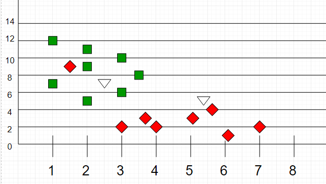
_Image source: [GeeksForGeeks](https://media.geeksforgeeks.org/wp-content/uploads/graph2-2.png)_
Here, as we can see, the classification of unknown points will be judged by their proximity to other points.
It is important to note that `K` is preferred to have odd values in order to break ties. Usually `K` is taken as `3` or `5`.
## References
- [k-nearest neighbors algorithm on Wikipedia](https://en.wikipedia.org/wiki/K-nearest_neighbors_algorithm)
================================================
FILE: src/algorithms/ml/knn/README.pt-BR.md
================================================
# Algoritmo de k-vizinhos mais próximos
_Leia isso em outros idiomas:_
[_English_](README.md)
O **algoritmo de k-vizinhos mais próximos (k-NN)** é um algoritmo de aprendizado de máquina supervisionado. É um algoritmo de classificação, determinando a classe de um vetor de amostra usando dados de amostra.
Na classificação k-NN, a saída é uma associação de classe. Um objeto é classificado por uma pluralidade de votos de seus vizinhos, com o objeto sendo atribuído à classe mais comum entre seus `k` vizinhos mais próximos (`k` é um inteiro positivo, tipicamente pequeno). Se `k = 1`, então o objeto é simplesmente atribuído à classe daquele único vizinho mais próximo.
The idea is to calculate the similarity between two data points on the basis of a distance metric. [Distância Euclidiana](https://github.com/trekhleb/javascript-algorithms/tree/master/src/algorithms/math/euclidean-distance) é usado principalmente para esta tarefa.

_Fonte: [Wikipedia](https://en.wikipedia.org/wiki/Euclidean_distance)_
O algoritmo é o seguinte:
1. Verifique se há erros como dados/rótulos inválidos.
2. Calcule a distância euclidiana de todos os pontos de dados nos dados de treinamento com o ponto de classificação
3. Classifique as distâncias dos pontos junto com suas classes em ordem crescente
4. Pegue as classes iniciais `K` e encontre o modo para obter a classe mais semelhante
5. Informe a classe mais semelhante
Aqui está uma visualização da classificação k-NN para melhor compreensão:

_Fonte: [Wikipedia](https://en.wikipedia.org/wiki/K-nearest_neighbors_algorithm)_
A amostra de teste (ponto verde) deve ser classificada em quadrados azuis ou em triângulos vermelhos. Se `k = 3` (círculo de linha sólida) é atribuído aos triângulos vermelhos porque existem `2` triângulos e apenas `1` quadrado dentro do círculo interno. Se `k = 5` (círculo de linha tracejada) é atribuído aos quadrados azuis (`3` quadrados vs. `2` triângulos dentro do círculo externo).
Outro exemplo de classificação k-NN:

_Fonte: [GeeksForGeeks](https://media.geeksforgeeks.org/wp-content/uploads/graph2-2.png)_
Aqui, como podemos ver, a classificação dos pontos desconhecidos será julgada pela proximidade com outros pontos.
É importante notar que `K` é preferível ter valores ímpares para desempate. Normalmente `K` é tomado como `3` ou `5`.
## Referências
- [k-nearest neighbors algorithm on Wikipedia](https://en.wikipedia.org/wiki/K-nearest_neighbors_algorithm)
================================================
FILE: src/algorithms/ml/knn/__test__/knn.test.js
================================================
import kNN from '../kNN';
describe('kNN', () => {
it('should throw an error on invalid data', () => {
expect(() => {
kNN();
}).toThrow('Either dataSet or labels or toClassify were not set');
});
it('should throw an error on invalid labels', () => {
const noLabels = () => {
kNN([[1, 1]]);
};
expect(noLabels).toThrow('Either dataSet or labels or toClassify were not set');
});
it('should throw an error on not giving classification vector', () => {
const noClassification = () => {
kNN([[1, 1]], [1]);
};
expect(noClassification).toThrow('Either dataSet or labels or toClassify were not set');
});
it('should throw an error on not giving classification vector', () => {
const inconsistent = () => {
kNN([[1, 1]], [1], [1]);
};
expect(inconsistent).toThrow('Matrices have different shapes');
});
it('should find the nearest neighbour', () => {
let dataSet;
let labels;
let toClassify;
let expectedClass;
dataSet = [[1, 1], [2, 2]];
labels = [1, 2];
toClassify = [1, 1];
expectedClass = 1;
expect(kNN(dataSet, labels, toClassify)).toBe(expectedClass);
dataSet = [[1, 1], [6, 2], [3, 3], [4, 5], [9, 2], [2, 4], [8, 7]];
labels = [1, 2, 1, 2, 1, 2, 1];
toClassify = [1.25, 1.25];
expectedClass = 1;
expect(kNN(dataSet, labels, toClassify)).toBe(expectedClass);
dataSet = [[1, 1], [6, 2], [3, 3], [4, 5], [9, 2], [2, 4], [8, 7]];
labels = [1, 2, 1, 2, 1, 2, 1];
toClassify = [1.25, 1.25];
expectedClass = 2;
expect(kNN(dataSet, labels, toClassify, 5)).toBe(expectedClass);
});
it('should find the nearest neighbour with equal distances', () => {
const dataSet = [[0, 0], [1, 1], [0, 2]];
const labels = [1, 3, 3];
const toClassify = [0, 1];
const expectedClass = 3;
expect(kNN(dataSet, labels, toClassify)).toBe(expectedClass);
});
it('should find the nearest neighbour in 3D space', () => {
const dataSet = [[0, 0, 0], [0, 1, 1], [0, 0, 2]];
const labels = [1, 3, 3];
const toClassify = [0, 0, 1];
const expectedClass = 3;
expect(kNN(dataSet, labels, toClassify)).toBe(expectedClass);
});
});
================================================
FILE: src/algorithms/ml/knn/kNN.js
================================================
/**
* Classifies the point in space based on k-nearest neighbors algorithm.
*
* @param {number[][]} dataSet - array of data points, i.e. [[0, 1], [3, 4], [5, 7]]
* @param {number[]} labels - array of classes (labels), i.e. [1, 1, 2]
* @param {number[]} toClassify - the point in space that needs to be classified, i.e. [5, 4]
* @param {number} k - number of nearest neighbors which will be taken into account (preferably odd)
* @return {number} - the class of the point
*/
import euclideanDistance from '../../math/euclidean-distance/euclideanDistance';
export default function kNN(
dataSet,
labels,
toClassify,
k = 3,
) {
if (!dataSet || !labels || !toClassify) {
throw new Error('Either dataSet or labels or toClassify were not set');
}
// Calculate distance from toClassify to each point for all dimensions in dataSet.
// Store distance and point's label into distances list.
const distances = [];
for (let i = 0; i < dataSet.length; i += 1) {
distances.push({
dist: euclideanDistance([dataSet[i]], [toClassify]),
label: labels[i],
});
}
// Sort distances list (from closer point to further ones).
// Take initial k values, count with class index
const kNearest = distances.sort((a, b) => {
if (a.dist === b.dist) {
return 0;
}
return a.dist < b.dist ? -1 : 1;
}).slice(0, k);
// Count the number of instances of each class in top k members.
const labelsCounter = {};
let topClass = 0;
let topClassCount = 0;
for (let i = 0; i < kNearest.length; i += 1) {
if (kNearest[i].label in labelsCounter) {
labelsCounter[kNearest[i].label] += 1;
} else {
labelsCounter[kNearest[i].label] = 1;
}
if (labelsCounter[kNearest[i].label] > topClassCount) {
topClassCount = labelsCounter[kNearest[i].label];
topClass = kNearest[i].label;
}
}
// Return the class with highest count.
return topClass;
}
================================================
FILE: src/algorithms/search/binary-search/README.es-ES.md
================================================
# Búsqueda binaria
_Lea esto en otros idiomas:_
[English](README.md)
[Português brasileiro](README.pt-BR.md).
En informática, la búsqueda binaria, también conocida como búsqueda de medio intervalo
búsqueda, búsqueda logarítmica, o corte binario, es un algoritmo de búsqueda
que encuentra la posición de un valor objetivo dentro de una matriz
ordenada. La búsqueda binaria compara el valor objetivo con el elemento central
de la matriz; si son desiguales, se elimina la mitad en la que
la mitad en la que no puede estar el objetivo se elimina y la búsqueda continúa
en la mitad restante hasta que tenga éxito. Si la búsqueda
termina con la mitad restante vacía, el objetivo no está
en la matriz.

## Complejidad
**Complejidad de tiempo**: `O(log(n))` - ya que dividimos el área de búsqueda en dos para cada
siguiente iteración.
## Referencias
- [Wikipedia](https://en.wikipedia.org/wiki/Binary_search_algorithm)
- [YouTube](https://www.youtube.com/watch?v=P3YID7liBug&index=29&list=PLLXdhg_r2hKA7DPDsunoDZ-Z769jWn4R8)
================================================
FILE: src/algorithms/search/binary-search/README.md
================================================
# Binary Search
_Read this in other languages:_
[Português brasileiro](README.pt-BR.md).
[Español](README.es-ES.md).
In computer science, binary search, also known as half-interval
search, logarithmic search, or binary chop, is a search algorithm
that finds the position of a target value within a sorted
array. Binary search compares the target value to the middle
element of the array; if they are unequal, the half in which
the target cannot lie is eliminated and the search continues
on the remaining half until it is successful. If the search
ends with the remaining half being empty, the target is not
in the array.

## Complexity
**Time Complexity**: `O(log(n))` - since we split search area by two for every
next iteration.
## References
- [Wikipedia](https://en.wikipedia.org/wiki/Binary_search_algorithm)
- [YouTube](https://www.youtube.com/watch?v=P3YID7liBug&index=29&list=PLLXdhg_r2hKA7DPDsunoDZ-Z769jWn4R8)
================================================
FILE: src/algorithms/search/binary-search/README.pt-BR.md
================================================
# Busca Binária
_Leia isso em outras línguas:_
[english](README.md).
[Español](README.es-ES.md).
Em ciência da computação, busca binária, também conhecida como busca de meio-intervalo, busca logarítmica ou corte binário, é um algoritmo de pesquisa
que encontra a posição de um elemento alvo dentro de um
vetor ordenado. O algoritmo compara o elemento alvo com o elemento central do vetor; se eles são diferentes, a metade em que
o elemento alvo não pode estar é eliminada e a busca continua
na metade remanescente até que o elemento alvo seja encontrado. Se a busca
terminar com a metade remanescente vazia, o elemento alvo não está presente no vetor.

## Complexidade
**Complexidade de Tempo**: `O(log(n))` - pois a área de busca é dividida por dois a cada iteração.
## Referências
- [Wikipedia](https://en.wikipedia.org/wiki/Binary_search_algorithm)
- [YouTube](https://www.youtube.com/watch?v=P3YID7liBug&index=29&list=PLLXdhg_r2hKA7DPDsunoDZ-Z769jWn4R8)
================================================
FILE: src/algorithms/search/binary-search/__test__/binarySearch.test.js
================================================
import binarySearch from '../binarySearch';
describe('binarySearch', () => {
it('should search number in sorted array', () => {
expect(binarySearch([], 1)).toBe(-1);
expect(binarySearch([1], 1)).toBe(0);
expect(binarySearch([1, 2], 1)).toBe(0);
expect(binarySearch([1, 2], 2)).toBe(1);
expect(binarySearch([1, 5, 10, 12], 1)).toBe(0);
expect(binarySearch([1, 5, 10, 12, 14, 17, 22, 100], 17)).toBe(5);
expect(binarySearch([1, 5, 10, 12, 14, 17, 22, 100], 1)).toBe(0);
expect(binarySearch([1, 5, 10, 12, 14, 17, 22, 100], 100)).toBe(7);
expect(binarySearch([1, 5, 10, 12, 14, 17, 22, 100], 0)).toBe(-1);
});
it('should search object in sorted array', () => {
const sortedArrayOfObjects = [
{ key: 1, value: 'value1' },
{ key: 2, value: 'value2' },
{ key: 3, value: 'value3' },
];
const comparator = (a, b) => {
if (a.key === b.key) return 0;
return a.key < b.key ? -1 : 1;
};
expect(binarySearch([], { key: 1 }, comparator)).toBe(-1);
expect(binarySearch(sortedArrayOfObjects, { key: 4 }, comparator)).toBe(-1);
expect(binarySearch(sortedArrayOfObjects, { key: 1 }, comparator)).toBe(0);
expect(binarySearch(sortedArrayOfObjects, { key: 2 }, comparator)).toBe(1);
expect(binarySearch(sortedArrayOfObjects, { key: 3 }, comparator)).toBe(2);
});
});
================================================
FILE: src/algorithms/search/binary-search/binarySearch.js
================================================
import Comparator from '../../../utils/comparator/Comparator';
/**
* Binary search implementation.
*
* @param {*[]} sortedArray
* @param {*} seekElement
* @param {function(a, b)} [comparatorCallback]
* @return {number}
*/
export default function binarySearch(sortedArray, seekElement, comparatorCallback) {
// Let's create comparator from the comparatorCallback function.
// Comparator object will give us common comparison methods like equal() and lessThan().
const comparator = new Comparator(comparatorCallback);
// These two indices will contain current array (sub-array) boundaries.
let startIndex = 0;
let endIndex = sortedArray.length - 1;
// Let's continue to split array until boundaries are collapsed
// and there is nothing to split anymore.
while (startIndex <= endIndex) {
// Let's calculate the index of the middle element.
const middleIndex = startIndex + Math.floor((endIndex - startIndex) / 2);
// If we've found the element just return its position.
if (comparator.equal(sortedArray[middleIndex], seekElement)) {
return middleIndex;
}
// Decide which half to choose for seeking next: left or right one.
if (comparator.lessThan(sortedArray[middleIndex], seekElement)) {
// Go to the right half of the array.
startIndex = middleIndex + 1;
} else {
// Go to the left half of the array.
endIndex = middleIndex - 1;
}
}
// Return -1 if we have not found anything.
return -1;
}
================================================
FILE: src/algorithms/search/interpolation-search/README.md
================================================
# Interpolation Search
**Interpolation search** is an algorithm for searching for a key in an array that
has been ordered by numerical values assigned to the keys (key values).
For example we have a sorted array of `n` uniformly distributed values `arr[]`,
and we need to write a function to search for a particular element `x` in the array.
**Linear Search** finds the element in `O(n)` time, **Jump Search** takes `O(√ n)` time
and **Binary Search** take `O(Log n)` time.
The **Interpolation Search** is an improvement over Binary Search for instances,
where the values in a sorted array are _uniformly_ distributed. Binary Search
always goes to the middle element to check. On the other hand, interpolation
search may go to different locations according to the value of the key being
searched. For example, if the value of the key is closer to the last element,
interpolation search is likely to start search toward the end side.
To find the position to be searched, it uses following formula:
```
// The idea of formula is to return higher value of pos
// when element to be searched is closer to arr[hi]. And
// smaller value when closer to arr[lo]
pos = lo + ((x - arr[lo]) * (hi - lo) / (arr[hi] - arr[Lo]))
arr[] - Array where elements need to be searched
x - Element to be searched
lo - Starting index in arr[]
hi - Ending index in arr[]
```
## Complexity
**Time complexity**: `O(log(log(n))`
## References
- [GeeksForGeeks](https://www.geeksforgeeks.org/interpolation-search/)
- [Wikipedia](https://en.wikipedia.org/wiki/Interpolation_search)
================================================
FILE: src/algorithms/search/interpolation-search/__test__/interpolationSearch.test.js
================================================
import interpolationSearch from '../interpolationSearch';
describe('interpolationSearch', () => {
it('should search elements in sorted array of numbers', () => {
expect(interpolationSearch([], 1)).toBe(-1);
expect(interpolationSearch([1], 1)).toBe(0);
expect(interpolationSearch([1], 0)).toBe(-1);
expect(interpolationSearch([1, 1], 1)).toBe(0);
expect(interpolationSearch([1, 2], 1)).toBe(0);
expect(interpolationSearch([1, 2], 2)).toBe(1);
expect(interpolationSearch([10, 20, 30, 40, 50], 40)).toBe(3);
expect(interpolationSearch([1, 2, 3, 4, 5, 6, 7, 8, 9, 10, 11, 12, 13, 14, 15], 14)).toBe(13);
expect(interpolationSearch([1, 6, 7, 8, 12, 13, 14, 19, 21, 23, 24, 24, 24, 300], 24)).toBe(10);
expect(interpolationSearch([1, 2, 3, 700, 800, 1200, 1300, 1400, 1900], 600)).toBe(-1);
expect(interpolationSearch([1, 2, 3, 700, 800, 1200, 1300, 1400, 1900], 1)).toBe(0);
expect(interpolationSearch([1, 2, 3, 700, 800, 1200, 1300, 1400, 1900], 2)).toBe(1);
expect(interpolationSearch([1, 2, 3, 700, 800, 1200, 1300, 1400, 1900], 3)).toBe(2);
expect(interpolationSearch([1, 2, 3, 700, 800, 1200, 1300, 1400, 1900], 700)).toBe(3);
expect(interpolationSearch([1, 2, 3, 700, 800, 1200, 1300, 1400, 1900], 800)).toBe(4);
expect(interpolationSearch([0, 2, 3, 700, 800, 1200, 1300, 1400, 1900], 1200)).toBe(5);
expect(interpolationSearch([1, 2, 3, 700, 800, 1200, 1300, 1400, 19000], 800)).toBe(4);
expect(interpolationSearch([0, 10, 11, 12, 13, 14, 15], 10)).toBe(1);
});
});
================================================
FILE: src/algorithms/search/interpolation-search/interpolationSearch.js
================================================
/**
* Interpolation search implementation.
*
* @param {*[]} sortedArray - sorted array with uniformly distributed values
* @param {*} seekElement
* @return {number}
*/
export default function interpolationSearch(sortedArray, seekElement) {
let leftIndex = 0;
let rightIndex = sortedArray.length - 1;
while (leftIndex <= rightIndex) {
const rangeDelta = sortedArray[rightIndex] - sortedArray[leftIndex];
const indexDelta = rightIndex - leftIndex;
const valueDelta = seekElement - sortedArray[leftIndex];
// If valueDelta is less then zero it means that there is no seek element
// exists in array since the lowest element from the range is already higher
// then seek element.
if (valueDelta < 0) {
return -1;
}
// If range delta is zero then subarray contains all the same numbers
// and thus there is nothing to search for unless this range is all
// consists of seek number.
if (!rangeDelta) {
// By doing this we're also avoiding division by zero while
// calculating the middleIndex later.
return sortedArray[leftIndex] === seekElement ? leftIndex : -1;
}
// Do interpolation of the middle index.
const middleIndex = leftIndex + Math.floor((valueDelta * indexDelta) / rangeDelta);
// If we've found the element just return its position.
if (sortedArray[middleIndex] === seekElement) {
return middleIndex;
}
// Decide which half to choose for seeking next: left or right one.
if (sortedArray[middleIndex] < seekElement) {
// Go to the right half of the array.
leftIndex = middleIndex + 1;
} else {
// Go to the left half of the array.
rightIndex = middleIndex - 1;
}
}
return -1;
}
================================================
FILE: src/algorithms/search/jump-search/README.md
================================================
# Jump Search
Like Binary Search, **Jump Search** (or **Block Search**) is a searching algorithm
for sorted arrays. The basic idea is to check fewer elements (than linear search)
by jumping ahead by fixed steps or skipping some elements in place of searching all
elements.
For example, suppose we have an array `arr[]` of size `n` and block (to be jumped)
of size `m`. Then we search at the indexes `arr[0]`, `arr[m]`, `arr[2 * m]`, ..., `arr[k * m]` and
so on. Once we find the interval `arr[k * m] < x < arr[(k+1) * m]`, we perform a
linear search operation from the index `k * m` to find the element `x`.
**What is the optimal block size to be skipped?**
In the worst case, we have to do `n/m` jumps and if the last checked value is
greater than the element to be searched for, we perform `m - 1` comparisons more
for linear search. Therefore the total number of comparisons in the worst case
will be `((n/m) + m - 1)`. The value of the function `((n/m) + m - 1)` will be
minimum when `m = √n`. Therefore, the best step size is `m = √n`.
## Complexity
**Time complexity**: `O(√n)` - because we do search by blocks of size `√n`.
## References
- [GeeksForGeeks](https://www.geeksforgeeks.org/jump-search/)
- [Wikipedia](https://en.wikipedia.org/wiki/Jump_search)
================================================
FILE: src/algorithms/search/jump-search/__test__/jumpSearch.test.js
================================================
import jumpSearch from '../jumpSearch';
describe('jumpSearch', () => {
it('should search for an element in sorted array', () => {
expect(jumpSearch([], 1)).toBe(-1);
expect(jumpSearch([1], 2)).toBe(-1);
expect(jumpSearch([1], 1)).toBe(0);
expect(jumpSearch([1, 2], 1)).toBe(0);
expect(jumpSearch([1, 2], 1)).toBe(0);
expect(jumpSearch([1, 1, 1], 1)).toBe(0);
expect(jumpSearch([1, 2, 5, 10, 20, 21, 24, 30, 48], 2)).toBe(1);
expect(jumpSearch([1, 2, 5, 10, 20, 21, 24, 30, 48], 0)).toBe(-1);
expect(jumpSearch([1, 2, 5, 10, 20, 21, 24, 30, 48], 0)).toBe(-1);
expect(jumpSearch([1, 2, 5, 10, 20, 21, 24, 30, 48], 7)).toBe(-1);
expect(jumpSearch([1, 2, 5, 10, 20, 21, 24, 30, 48], 5)).toBe(2);
expect(jumpSearch([1, 2, 5, 10, 20, 21, 24, 30, 48], 20)).toBe(4);
expect(jumpSearch([1, 2, 5, 10, 20, 21, 24, 30, 48], 30)).toBe(7);
expect(jumpSearch([1, 2, 5, 10, 20, 21, 24, 30, 48], 48)).toBe(8);
});
it('should search object in sorted array', () => {
const sortedArrayOfObjects = [
{ key: 1, value: 'value1' },
{ key: 2, value: 'value2' },
{ key: 3, value: 'value3' },
];
const comparator = (a, b) => {
if (a.key === b.key) return 0;
return a.key < b.key ? -1 : 1;
};
expect(jumpSearch([], { key: 1 }, comparator)).toBe(-1);
expect(jumpSearch(sortedArrayOfObjects, { key: 4 }, comparator)).toBe(-1);
expect(jumpSearch(sortedArrayOfObjects, { key: 1 }, comparator)).toBe(0);
expect(jumpSearch(sortedArrayOfObjects, { key: 2 }, comparator)).toBe(1);
expect(jumpSearch(sortedArrayOfObjects, { key: 3 }, comparator)).toBe(2);
});
});
================================================
FILE: src/algorithms/search/jump-search/jumpSearch.js
================================================
import Comparator from '../../../utils/comparator/Comparator';
/**
* Jump (block) search implementation.
*
* @param {*[]} sortedArray
* @param {*} seekElement
* @param {function(a, b)} [comparatorCallback]
* @return {number}
*/
export default function jumpSearch(sortedArray, seekElement, comparatorCallback) {
const comparator = new Comparator(comparatorCallback);
const arraySize = sortedArray.length;
if (!arraySize) {
// We can't find anything in empty array.
return -1;
}
// Calculate optimal jump size.
// Total number of comparisons in the worst case will be ((arraySize/jumpSize) + jumpSize - 1).
// The value of the function ((arraySize/jumpSize) + jumpSize - 1) will be minimum
// when jumpSize = √array.length.
const jumpSize = Math.floor(Math.sqrt(arraySize));
// Find the block where the seekElement belong to.
let blockStart = 0;
let blockEnd = jumpSize;
while (comparator.greaterThan(seekElement, sortedArray[Math.min(blockEnd, arraySize) - 1])) {
// Jump to the next block.
blockStart = blockEnd;
blockEnd += jumpSize;
// If our next block is out of array then we couldn't found the element.
if (blockStart > arraySize) {
return -1;
}
}
// Do linear search for seekElement in subarray starting from blockStart.
let currentIndex = blockStart;
while (currentIndex < Math.min(blockEnd, arraySize)) {
if (comparator.equal(sortedArray[currentIndex], seekElement)) {
return currentIndex;
}
currentIndex += 1;
}
return -1;
}
================================================
FILE: src/algorithms/search/linear-search/README.md
================================================
# Linear Search
_Read this in other languages:_
[Português brasileiro](README.pt-BR.md).
In computer science, linear search or sequential search is a
method for finding a target value within a list. It sequentially
checks each element of the list for the target value until a
match is found or until all the elements have been searched.
Linear search runs in at worst linear time and makes at most `n`
comparisons, where `n` is the length of the list.
## Complexity
**Time Complexity**: `O(n)` - since in worst case we're checking each element
exactly once.
## References
- [Wikipedia](https://en.wikipedia.org/wiki/Linear_search)
- [TutorialsPoint](https://www.tutorialspoint.com/data_structures_algorithms/linear_search_algorithm.htm)
- [Youtube](https://www.youtube.com/watch?v=SGU9duLE30w)
================================================
FILE: src/algorithms/search/linear-search/README.pt-BR.md
================================================
# Busca Linear
_Leia isso em outras línguas:_
[english](README.md).
Na Ciência da Computação, busca linear ou busca sequencial é um método para encontrar um elemento alvo em uma lista.
O algoritmo verifica sequencialmente cada elemento da lista procurando o elemento alvo até ele ser encontrado ou até ter verificado todos os elementos.
A Busca linear realiza no máximo `n` comparações, onde `n` é o tamanho da lista.

## Complexidade
**Complexidade de Tempo**: `O(n)` - pois no pior caso devemos verificar cada elemento exatamente uma vez.
## Referências
- [Wikipedia](https://en.wikipedia.org/wiki/Linear_search)
- [TutorialsPoint](https://www.tutorialspoint.com/data_structures_algorithms/linear_search_algorithm.htm)
- [Youtube](https://www.youtube.com/watch?v=SGU9duLE30w)
================================================
FILE: src/algorithms/search/linear-search/__test__/linearSearch.test.js
================================================
import linearSearch from '../linearSearch';
describe('linearSearch', () => {
it('should search all numbers in array', () => {
const array = [1, 2, 4, 6, 2];
expect(linearSearch(array, 10)).toEqual([]);
expect(linearSearch(array, 1)).toEqual([0]);
expect(linearSearch(array, 2)).toEqual([1, 4]);
});
it('should search all strings in array', () => {
const array = ['a', 'b', 'a'];
expect(linearSearch(array, 'c')).toEqual([]);
expect(linearSearch(array, 'b')).toEqual([1]);
expect(linearSearch(array, 'a')).toEqual([0, 2]);
});
it('should search through objects as well', () => {
const comparatorCallback = (a, b) => {
if (a.key === b.key) {
return 0;
}
return a.key <= b.key ? -1 : 1;
};
const array = [
{ key: 5 },
{ key: 6 },
{ key: 7 },
{ key: 6 },
];
expect(linearSearch(array, { key: 10 }, comparatorCallback)).toEqual([]);
expect(linearSearch(array, { key: 5 }, comparatorCallback)).toEqual([0]);
expect(linearSearch(array, { key: 6 }, comparatorCallback)).toEqual([1, 3]);
});
});
================================================
FILE: src/algorithms/search/linear-search/linearSearch.js
================================================
import Comparator from '../../../utils/comparator/Comparator';
/**
* Linear search implementation.
*
* @param {*[]} array
* @param {*} seekElement
* @param {function(a, b)} [comparatorCallback]
* @return {number[]}
*/
export default function linearSearch(array, seekElement, comparatorCallback) {
const comparator = new Comparator(comparatorCallback);
const foundIndices = [];
array.forEach((element, index) => {
if (comparator.equal(element, seekElement)) {
foundIndices.push(index);
}
});
return foundIndices;
}
================================================
FILE: src/algorithms/sets/cartesian-product/README.md
================================================
# Cartesian Product
In set theory a Cartesian product is a mathematical operation that returns a set
(or product set or simply product) from multiple sets. That is, for sets A and B,
the Cartesian product A × B is the set of all ordered pairs (a, b)
where a ∈ A and b ∈ B.
Cartesian product `AxB` of two sets `A={x,y,z}` and `B={1,2,3}`

## References
[Wikipedia](https://en.wikipedia.org/wiki/Cartesian_product)
================================================
FILE: src/algorithms/sets/cartesian-product/__test__/cartesianProduct.test.js
================================================
import cartesianProduct from '../cartesianProduct';
describe('cartesianProduct', () => {
it('should return null if there is not enough info for calculation', () => {
const product1 = cartesianProduct([1], null);
const product2 = cartesianProduct([], null);
expect(product1).toBeNull();
expect(product2).toBeNull();
});
it('should calculate the product of two sets', () => {
const product1 = cartesianProduct([1], [1]);
const product2 = cartesianProduct([1, 2], [3, 5]);
expect(product1).toEqual([[1, 1]]);
expect(product2).toEqual([[1, 3], [1, 5], [2, 3], [2, 5]]);
});
});
================================================
FILE: src/algorithms/sets/cartesian-product/cartesianProduct.js
================================================
/**
* Generates Cartesian Product of two sets.
* @param {*[]} setA
* @param {*[]} setB
* @return {*[]}
*/
export default function cartesianProduct(setA, setB) {
// Check if input sets are not empty.
// Otherwise return null since we can't generate Cartesian Product out of them.
if (!setA || !setB || !setA.length || !setB.length) {
return null;
}
// Init product set.
const product = [];
// Now, let's go through all elements of a first and second set and form all possible pairs.
for (let indexA = 0; indexA < setA.length; indexA += 1) {
for (let indexB = 0; indexB < setB.length; indexB += 1) {
// Add current product pair to the product set.
product.push([setA[indexA], setB[indexB]]);
}
}
// Return cartesian product set.
return product;
}
================================================
FILE: src/algorithms/sets/combination-sum/README.md
================================================
# Combination Sum Problem
Given a **set** of candidate numbers (`candidates`) **(without duplicates)** and
a target number (`target`), find all unique combinations in `candidates` where
the candidate numbers sums to `target`.
The **same** repeated number may be chosen from `candidates` unlimited number
of times.
**Note:**
- All numbers (including `target`) will be positive integers.
- The solution set must not contain duplicate combinations.
## Examples
```
Input: candidates = [2,3,6,7], target = 7,
A solution set is:
[
[7],
[2,2,3]
]
```
```
Input: candidates = [2,3,5], target = 8,
A solution set is:
[
[2,2,2,2],
[2,3,3],
[3,5]
]
```
## Explanations
Since the problem is to get all the possible results, not the best or the
number of result, thus we don’t need to consider DP (dynamic programming),
backtracking approach using recursion is needed to handle it.
Here is an example of decision tree for the situation when `candidates = [2, 3]` and `target = 6`:
```
0
/ \
+2 +3
/ \ \
+2 +3 +3
/ \ / \ \
+2 ✘ ✘ ✘ ✓
/ \
✓ ✘
```
## References
- [LeetCode](https://leetcode.com/problems/combination-sum/description/)
================================================
FILE: src/algorithms/sets/combination-sum/__test__/combinationSum.test.js
================================================
import combinationSum from '../combinationSum';
describe('combinationSum', () => {
it('should find all combinations with specific sum', () => {
expect(combinationSum([1], 4)).toEqual([
[1, 1, 1, 1],
]);
expect(combinationSum([2, 3, 6, 7], 7)).toEqual([
[2, 2, 3],
[7],
]);
expect(combinationSum([2, 3, 5], 8)).toEqual([
[2, 2, 2, 2],
[2, 3, 3],
[3, 5],
]);
expect(combinationSum([2, 5], 3)).toEqual([]);
expect(combinationSum([], 3)).toEqual([]);
});
});
================================================
FILE: src/algorithms/sets/combination-sum/combinationSum.js
================================================
/**
* @param {number[]} candidates - candidate numbers we're picking from.
* @param {number} remainingSum - remaining sum after adding candidates to currentCombination.
* @param {number[][]} finalCombinations - resulting list of combinations.
* @param {number[]} currentCombination - currently explored candidates.
* @param {number} startFrom - index of the candidate to start further exploration from.
* @return {number[][]}
*/
function combinationSumRecursive(
candidates,
remainingSum,
finalCombinations = [],
currentCombination = [],
startFrom = 0,
) {
if (remainingSum < 0) {
// By adding another candidate we've gone below zero.
// This would mean that the last candidate was not acceptable.
return finalCombinations;
}
if (remainingSum === 0) {
// If after adding the previous candidate our remaining sum
// became zero - we need to save the current combination since it is one
// of the answers we're looking for.
finalCombinations.push(currentCombination.slice());
return finalCombinations;
}
// If we haven't reached zero yet let's continue to add all
// possible candidates that are left.
for (let candidateIndex = startFrom; candidateIndex < candidates.length; candidateIndex += 1) {
const currentCandidate = candidates[candidateIndex];
// Let's try to add another candidate.
currentCombination.push(currentCandidate);
// Explore further option with current candidate being added.
combinationSumRecursive(
candidates,
remainingSum - currentCandidate,
finalCombinations,
currentCombination,
candidateIndex,
);
// BACKTRACKING.
// Let's get back, exclude current candidate and try another ones later.
currentCombination.pop();
}
return finalCombinations;
}
/**
* Backtracking algorithm of finding all possible combination for specific sum.
*
* @param {number[]} candidates
* @param {number} target
* @return {number[][]}
*/
export default function combinationSum(candidates, target) {
return combinationSumRecursive(candidates, target);
}
================================================
FILE: src/algorithms/sets/combinations/README.md
================================================
# Combinations
When the order doesn't matter, it is a **Combination**.
When the order **does** matter it is a **Permutation**.
**"My fruit salad is a combination of apples, grapes and bananas"**
We don't care what order the fruits are in, they could also be
"bananas, grapes and apples" or "grapes, apples and bananas",
its the same fruit salad.
## Combinations without repetitions
This is how lotteries work. The numbers are drawn one at a
time, and if we have the lucky numbers (no matter what order)
we win!
No Repetition: such as lottery numbers `(2,14,15,27,30,33)`
**Number of combinations**
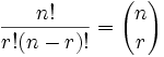
where `n` is the number of things to choose from, and we choose `r` of them,
no repetition, order doesn't matter.
It is often called "n choose r" (such as "16 choose 3"). And is also known as the Binomial Coefficient.
## Combinations with repetitions
Repetition is Allowed: such as coins in your pocket `(5,5,5,10,10)`
Or let us say there are five flavours of ice cream:
`banana`, `chocolate`, `lemon`, `strawberry` and `vanilla`.
We can have three scoops. How many variations will there be?
Let's use letters for the flavours: `{b, c, l, s, v}`.
Example selections include:
- `{c, c, c}` (3 scoops of chocolate)
- `{b, l, v}` (one each of banana, lemon and vanilla)
- `{b, v, v}` (one of banana, two of vanilla)
**Number of combinations**
Where `n` is the number of things to choose from, and we
choose `r` of them. Repetition allowed,
order doesn't matter.
## Cheatsheet


| | |
| --- | --- |
| |  |
*Made with [okso.app](https://okso.app)*
## References
- [Math Is Fun](https://www.mathsisfun.com/combinatorics/combinations-permutations.html)
- [Permutations/combinations cheat sheets](https://medium.com/@trekhleb/permutations-combinations-algorithms-cheat-sheet-68c14879aba5)
================================================
FILE: src/algorithms/sets/combinations/__test__/combineWithRepetitions.test.js
================================================
import combineWithRepetitions from '../combineWithRepetitions';
import factorial from '../../../math/factorial/factorial';
describe('combineWithRepetitions', () => {
it('should combine string with repetitions', () => {
expect(combineWithRepetitions(['A'], 1)).toEqual([
['A'],
]);
expect(combineWithRepetitions(['A', 'B'], 1)).toEqual([
['A'],
['B'],
]);
expect(combineWithRepetitions(['A', 'B'], 2)).toEqual([
['A', 'A'],
['A', 'B'],
['B', 'B'],
]);
expect(combineWithRepetitions(['A', 'B'], 3)).toEqual([
['A', 'A', 'A'],
['A', 'A', 'B'],
['A', 'B', 'B'],
['B', 'B', 'B'],
]);
expect(combineWithRepetitions(['A', 'B', 'C'], 2)).toEqual([
['A', 'A'],
['A', 'B'],
['A', 'C'],
['B', 'B'],
['B', 'C'],
['C', 'C'],
]);
expect(combineWithRepetitions(['A', 'B', 'C'], 3)).toEqual([
['A', 'A', 'A'],
['A', 'A', 'B'],
['A', 'A', 'C'],
['A', 'B', 'B'],
['A', 'B', 'C'],
['A', 'C', 'C'],
['B', 'B', 'B'],
['B', 'B', 'C'],
['B', 'C', 'C'],
['C', 'C', 'C'],
]);
const combinationOptions = ['A', 'B', 'C', 'D', 'E', 'F', 'G', 'H'];
const combinationSlotsNumber = 4;
const combinations = combineWithRepetitions(combinationOptions, combinationSlotsNumber);
const n = combinationOptions.length;
const r = combinationSlotsNumber;
const expectedNumberOfCombinations = factorial((r + n) - 1) / (factorial(r) * factorial(n - 1));
expect(combinations.length).toBe(expectedNumberOfCombinations);
});
});
================================================
FILE: src/algorithms/sets/combinations/__test__/combineWithoutRepetitions.test.js
================================================
import combineWithoutRepetitions from '../combineWithoutRepetitions';
import factorial from '../../../math/factorial/factorial';
import pascalTriangle from '../../../math/pascal-triangle/pascalTriangle';
describe('combineWithoutRepetitions', () => {
it('should combine string without repetitions', () => {
expect(combineWithoutRepetitions(['A', 'B'], 3)).toEqual([]);
expect(combineWithoutRepetitions(['A', 'B'], 1)).toEqual([
['A'],
['B'],
]);
expect(combineWithoutRepetitions(['A'], 1)).toEqual([
['A'],
]);
expect(combineWithoutRepetitions(['A', 'B'], 2)).toEqual([
['A', 'B'],
]);
expect(combineWithoutRepetitions(['A', 'B', 'C'], 2)).toEqual([
['A', 'B'],
['A', 'C'],
['B', 'C'],
]);
expect(combineWithoutRepetitions(['A', 'B', 'C'], 3)).toEqual([
['A', 'B', 'C'],
]);
expect(combineWithoutRepetitions(['A', 'B', 'C', 'D'], 3)).toEqual([
['A', 'B', 'C'],
['A', 'B', 'D'],
['A', 'C', 'D'],
['B', 'C', 'D'],
]);
expect(combineWithoutRepetitions(['A', 'B', 'C', 'D', 'E'], 3)).toEqual([
['A', 'B', 'C'],
['A', 'B', 'D'],
['A', 'B', 'E'],
['A', 'C', 'D'],
['A', 'C', 'E'],
['A', 'D', 'E'],
['B', 'C', 'D'],
['B', 'C', 'E'],
['B', 'D', 'E'],
['C', 'D', 'E'],
]);
const combinationOptions = ['A', 'B', 'C', 'D', 'E', 'F', 'G', 'H'];
const combinationSlotsNumber = 4;
const combinations = combineWithoutRepetitions(combinationOptions, combinationSlotsNumber);
const n = combinationOptions.length;
const r = combinationSlotsNumber;
const expectedNumberOfCombinations = factorial(n) / (factorial(r) * factorial(n - r));
expect(combinations.length).toBe(expectedNumberOfCombinations);
// This one is just to see one of the way of Pascal's triangle application.
expect(combinations.length).toBe(pascalTriangle(n)[r]);
});
});
================================================
FILE: src/algorithms/sets/combinations/combineWithRepetitions.js
================================================
/**
* @param {*[]} comboOptions
* @param {number} comboLength
* @return {*[]}
*/
export default function combineWithRepetitions(comboOptions, comboLength) {
// If the length of the combination is 1 then each element of the original array
// is a combination itself.
if (comboLength === 1) {
return comboOptions.map((comboOption) => [comboOption]);
}
// Init combinations array.
const combos = [];
// Remember characters one by one and concatenate them to combinations of smaller lengths.
// We don't extract elements here because the repetitions are allowed.
comboOptions.forEach((currentOption, optionIndex) => {
// Generate combinations of smaller size.
const smallerCombos = combineWithRepetitions(
comboOptions.slice(optionIndex),
comboLength - 1,
);
// Concatenate currentOption with all combinations of smaller size.
smallerCombos.forEach((smallerCombo) => {
combos.push([currentOption].concat(smallerCombo));
});
});
return combos;
}
================================================
FILE: src/algorithms/sets/combinations/combineWithoutRepetitions.js
================================================
/**
* @param {*[]} comboOptions
* @param {number} comboLength
* @return {*[]}
*/
export default function combineWithoutRepetitions(comboOptions, comboLength) {
// If the length of the combination is 1 then each element of the original array
// is a combination itself.
if (comboLength === 1) {
return comboOptions.map((comboOption) => [comboOption]);
}
// Init combinations array.
const combos = [];
// Extract characters one by one and concatenate them to combinations of smaller lengths.
// We need to extract them because we don't want to have repetitions after concatenation.
comboOptions.forEach((currentOption, optionIndex) => {
// Generate combinations of smaller size.
const smallerCombos = combineWithoutRepetitions(
comboOptions.slice(optionIndex + 1),
comboLength - 1,
);
// Concatenate currentOption with all combinations of smaller size.
smallerCombos.forEach((smallerCombo) => {
combos.push([currentOption].concat(smallerCombo));
});
});
return combos;
}
================================================
FILE: src/algorithms/sets/fisher-yates/README.md
================================================
# Fisher–Yates shuffle
The Fisher–Yates shuffle is an algorithm for generating a random
permutation of a finite sequence—in plain terms, the algorithm
shuffles the sequence. The algorithm effectively puts all the
elements into a hat; it continually determines the next element
by randomly drawing an element from the hat until no elements
remain. The algorithm produces an unbiased permutation: every
permutation is equally likely. The modern version of the
algorithm is efficient: it takes time proportional to the
number of items being shuffled and shuffles them in place.
## References
[Wikipedia](https://en.wikipedia.org/wiki/Fisher%E2%80%93Yates_shuffle)
================================================
FILE: src/algorithms/sets/fisher-yates/__test__/fisherYates.test.js
================================================
import fisherYates from '../fisherYates';
import { sortedArr } from '../../../sorting/SortTester';
import QuickSort from '../../../sorting/quick-sort/QuickSort';
describe('fisherYates', () => {
it('should shuffle small arrays', () => {
expect(fisherYates([])).toEqual([]);
expect(fisherYates([1])).toEqual([1]);
});
it('should shuffle array randomly', () => {
const shuffledArray = fisherYates(sortedArr);
const sorter = new QuickSort();
expect(shuffledArray.length).toBe(sortedArr.length);
expect(shuffledArray).not.toEqual(sortedArr);
expect(sorter.sort(shuffledArray)).toEqual(sortedArr);
});
});
================================================
FILE: src/algorithms/sets/fisher-yates/fisherYates.js
================================================
/**
* @param {*[]} originalArray
* @return {*[]}
*/
export default function fisherYates(originalArray) {
// Clone array from preventing original array from modification (for testing purpose).
const array = originalArray.slice(0);
for (let i = (array.length - 1); i > 0; i -= 1) {
const randomIndex = Math.floor(Math.random() * (i + 1));
[array[i], array[randomIndex]] = [array[randomIndex], array[i]];
}
return array;
}
================================================
FILE: src/algorithms/sets/knapsack-problem/Knapsack.js
================================================
import MergeSort from '../../sorting/merge-sort/MergeSort';
export default class Knapsack {
/**
* @param {KnapsackItem[]} possibleItems
* @param {number} weightLimit
*/
constructor(possibleItems, weightLimit) {
this.selectedItems = [];
this.weightLimit = weightLimit;
this.possibleItems = possibleItems;
}
sortPossibleItemsByWeight() {
this.possibleItems = new MergeSort({
/**
* @var KnapsackItem itemA
* @var KnapsackItem itemB
*/
compareCallback: (itemA, itemB) => {
if (itemA.weight === itemB.weight) {
return 0;
}
return itemA.weight < itemB.weight ? -1 : 1;
},
}).sort(this.possibleItems);
}
sortPossibleItemsByValue() {
this.possibleItems = new MergeSort({
/**
* @var KnapsackItem itemA
* @var KnapsackItem itemB
*/
compareCallback: (itemA, itemB) => {
if (itemA.value === itemB.value) {
return 0;
}
return itemA.value > itemB.value ? -1 : 1;
},
}).sort(this.possibleItems);
}
sortPossibleItemsByValuePerWeightRatio() {
this.possibleItems = new MergeSort({
/**
* @var KnapsackItem itemA
* @var KnapsackItem itemB
*/
compareCallback: (itemA, itemB) => {
if (itemA.valuePerWeightRatio === itemB.valuePerWeightRatio) {
return 0;
}
return itemA.valuePerWeightRatio > itemB.valuePerWeightRatio ? -1 : 1;
},
}).sort(this.possibleItems);
}
// Solve 0/1 knapsack problem
// Dynamic Programming approach.
solveZeroOneKnapsackProblem() {
// We do two sorts because in case of equal weights but different values
// we need to take the most valuable items first.
this.sortPossibleItemsByValue();
this.sortPossibleItemsByWeight();
this.selectedItems = [];
// Create knapsack values matrix.
const numberOfRows = this.possibleItems.length;
const numberOfColumns = this.weightLimit;
const knapsackMatrix = Array(numberOfRows).fill(null).map(() => {
return Array(numberOfColumns + 1).fill(null);
});
// Fill the first column with zeros since it would mean that there is
// no items we can add to knapsack in case if weight limitation is zero.
for (let itemIndex = 0; itemIndex < this.possibleItems.length; itemIndex += 1) {
knapsackMatrix[itemIndex][0] = 0;
}
// Fill the first row with max possible values we would get by just adding
// or not adding the first item to the knapsack.
for (let weightIndex = 1; weightIndex <= this.weightLimit; weightIndex += 1) {
const itemIndex = 0;
const itemWeight = this.possibleItems[itemIndex].weight;
const itemValue = this.possibleItems[itemIndex].value;
knapsackMatrix[itemIndex][weightIndex] = itemWeight <= weightIndex ? itemValue : 0;
}
// Go through combinations of how we may add items to knapsack and
// define what weight/value we would receive using Dynamic Programming
// approach.
for (let itemIndex = 1; itemIndex < this.possibleItems.length; itemIndex += 1) {
for (let weightIndex = 1; weightIndex <= this.weightLimit; weightIndex += 1) {
const currentItemWeight = this.possibleItems[itemIndex].weight;
const currentItemValue = this.possibleItems[itemIndex].value;
if (currentItemWeight > weightIndex) {
// In case if item's weight is bigger then currently allowed weight
// then we can't add it to knapsack and the max possible value we can
// gain at the moment is the max value we got for previous item.
knapsackMatrix[itemIndex][weightIndex] = knapsackMatrix[itemIndex - 1][weightIndex];
} else {
// Else we need to consider the max value we can gain at this point by adding
// current value or just by keeping the previous item for current weight.
knapsackMatrix[itemIndex][weightIndex] = Math.max(
currentItemValue + knapsackMatrix[itemIndex - 1][weightIndex - currentItemWeight],
knapsackMatrix[itemIndex - 1][weightIndex],
);
}
}
}
// Now let's trace back the knapsack matrix to see what items we're going to add
// to the knapsack.
let itemIndex = this.possibleItems.length - 1;
let weightIndex = this.weightLimit;
while (itemIndex > 0) {
const currentItem = this.possibleItems[itemIndex];
const prevItem = this.possibleItems[itemIndex - 1];
// Check if matrix value came from top (from previous item).
// In this case this would mean that we need to include previous item
// to the list of selected items.
if (
knapsackMatrix[itemIndex][weightIndex]
&& knapsackMatrix[itemIndex][weightIndex] === knapsackMatrix[itemIndex - 1][weightIndex]
) {
// Check if there are several items with the same weight but with the different values.
// We need to add highest item in the matrix that is possible to get the highest value.
const prevSumValue = knapsackMatrix[itemIndex - 1][weightIndex];
const prevPrevSumValue = knapsackMatrix[itemIndex - 2][weightIndex];
if (
!prevSumValue
|| (prevSumValue && prevPrevSumValue !== prevSumValue)
) {
this.selectedItems.push(prevItem);
}
} else if (knapsackMatrix[itemIndex - 1][weightIndex - currentItem.weight]) {
this.selectedItems.push(prevItem);
weightIndex -= currentItem.weight;
}
itemIndex -= 1;
}
}
// Solve unbounded knapsack problem.
// Greedy approach.
solveUnboundedKnapsackProblem() {
this.sortPossibleItemsByValue();
this.sortPossibleItemsByValuePerWeightRatio();
for (let itemIndex = 0; itemIndex < this.possibleItems.length; itemIndex += 1) {
if (this.totalWeight < this.weightLimit) {
const currentItem = this.possibleItems[itemIndex];
// Detect how much of current items we can push to knapsack.
const availableWeight = this.weightLimit - this.totalWeight;
const maxPossibleItemsCount = Math.floor(availableWeight / currentItem.weight);
if (maxPossibleItemsCount > currentItem.itemsInStock) {
// If we have more items in stock then it is allowed to add
// let's add the maximum allowed number of them.
currentItem.quantity = currentItem.itemsInStock;
} else if (maxPossibleItemsCount) {
// In case if we don't have specified number of items in stock
// let's add only items we have in stock.
currentItem.quantity = maxPossibleItemsCount;
}
this.selectedItems.push(currentItem);
}
}
}
get totalValue() {
/** @var {KnapsackItem} item */
return this.selectedItems.reduce((accumulator, item) => {
return accumulator + item.totalValue;
}, 0);
}
get totalWeight() {
/** @var {KnapsackItem} item */
return this.selectedItems.reduce((accumulator, item) => {
return accumulator + item.totalWeight;
}, 0);
}
}
================================================
FILE: src/algorithms/sets/knapsack-problem/KnapsackItem.js
================================================
export default class KnapsackItem {
/**
* @param {Object} itemSettings - knapsack item settings,
* @param {number} itemSettings.value - value of the item.
* @param {number} itemSettings.weight - weight of the item.
* @param {number} itemSettings.itemsInStock - how many items are available to be added.
*/
constructor({ value, weight, itemsInStock = 1 }) {
this.value = value;
this.weight = weight;
this.itemsInStock = itemsInStock;
// Actual number of items that is going to be added to knapsack.
this.quantity = 1;
}
get totalValue() {
return this.value * this.quantity;
}
get totalWeight() {
return this.weight * this.quantity;
}
// This coefficient shows how valuable the 1 unit of weight is
// for current item.
get valuePerWeightRatio() {
return this.value / this.weight;
}
toString() {
return `v${this.value} w${this.weight} x ${this.quantity}`;
}
}
================================================
FILE: src/algorithms/sets/knapsack-problem/README.md
================================================
# Knapsack Problem
The knapsack problem or rucksack problem is a problem in
combinatorial optimization: Given a set of items, each with
a weight and a value, determine the number of each item to
include in a collection so that the total weight is less
than or equal to a given limit and the total value is as
large as possible.
It derives its name from the problem faced by someone who is
constrained by a fixed-size knapsack and must fill it with the
most valuable items.
Example of a one-dimensional (constraint) knapsack problem:
which boxes should be chosen to maximize the amount of money
while still keeping the overall weight under or equal to 15 kg?

## Definition
### 0/1 knapsack problem
The most common problem being solved is the **0/1 knapsack problem**,
which restricts the number `xi` of copies of each kind of item to zero or one.
Given a set of n items numbered from `1` up to `n`, each with a
weight `wi` and a value `vi`, along with a maximum weight
capacity `W`,
maximize 
subject to 
and 
Here `xi` represents the number of instances of item `i` to
include in the knapsack. Informally, the problem is to maximize
the sum of the values of the items in the knapsack so that the
sum of the weights is less than or equal to the knapsack's
capacity.
### Bounded knapsack problem (BKP)
The **bounded knapsack problem (BKP)** removes the restriction
that there is only one of each item, but restricts the number
`xi` of copies of each kind of item to a maximum non-negative
integer value `c`:
maximize 
subject to 
and 
### Unbounded knapsack problem (UKP)
The **unbounded knapsack problem (UKP)** places no upper bound
on the number of copies of each kind of item and can be
formulated as above except for that the only restriction
on `xi` is that it is a non-negative integer.
maximize 
subject to 
and 
## References
- [Wikipedia](https://en.wikipedia.org/wiki/Knapsack_problem)
- [0/1 Knapsack Problem on YouTube](https://www.youtube.com/watch?v=8LusJS5-AGo&list=PLLXdhg_r2hKA7DPDsunoDZ-Z769jWn4R8)
================================================
FILE: src/algorithms/sets/knapsack-problem/__test__/Knapsack.test.js
================================================
import Knapsack from '../Knapsack';
import KnapsackItem from '../KnapsackItem';
describe('Knapsack', () => {
it('should solve 0/1 knapsack problem', () => {
const possibleKnapsackItems = [
new KnapsackItem({ value: 1, weight: 1 }),
new KnapsackItem({ value: 4, weight: 3 }),
new KnapsackItem({ value: 5, weight: 4 }),
new KnapsackItem({ value: 7, weight: 5 }),
];
const maxKnapsackWeight = 7;
const knapsack = new Knapsack(possibleKnapsackItems, maxKnapsackWeight);
knapsack.solveZeroOneKnapsackProblem();
expect(knapsack.totalValue).toBe(9);
expect(knapsack.totalWeight).toBe(7);
expect(knapsack.selectedItems.length).toBe(2);
expect(knapsack.selectedItems[0].toString()).toBe('v5 w4 x 1');
expect(knapsack.selectedItems[1].toString()).toBe('v4 w3 x 1');
});
it('should solve 0/1 knapsack problem regardless of items order', () => {
const possibleKnapsackItems = [
new KnapsackItem({ value: 5, weight: 4 }),
new KnapsackItem({ value: 1, weight: 1 }),
new KnapsackItem({ value: 7, weight: 5 }),
new KnapsackItem({ value: 4, weight: 3 }),
];
const maxKnapsackWeight = 7;
const knapsack = new Knapsack(possibleKnapsackItems, maxKnapsackWeight);
knapsack.solveZeroOneKnapsackProblem();
expect(knapsack.totalValue).toBe(9);
expect(knapsack.totalWeight).toBe(7);
expect(knapsack.selectedItems.length).toBe(2);
expect(knapsack.selectedItems[0].toString()).toBe('v5 w4 x 1');
expect(knapsack.selectedItems[1].toString()).toBe('v4 w3 x 1');
});
it('should solve 0/1 knapsack problem with impossible items set', () => {
const possibleKnapsackItems = [
new KnapsackItem({ value: 5, weight: 40 }),
new KnapsackItem({ value: 1, weight: 10 }),
new KnapsackItem({ value: 7, weight: 50 }),
new KnapsackItem({ value: 4, weight: 30 }),
];
const maxKnapsackWeight = 7;
const knapsack = new Knapsack(possibleKnapsackItems, maxKnapsackWeight);
knapsack.solveZeroOneKnapsackProblem();
expect(knapsack.totalValue).toBe(0);
expect(knapsack.totalWeight).toBe(0);
expect(knapsack.selectedItems.length).toBe(0);
});
it('should solve 0/1 knapsack problem with all equal weights', () => {
const possibleKnapsackItems = [
new KnapsackItem({ value: 5, weight: 1 }),
new KnapsackItem({ value: 1, weight: 1 }),
new KnapsackItem({ value: 7, weight: 1 }),
new KnapsackItem({ value: 4, weight: 1 }),
new KnapsackItem({ value: 4, weight: 1 }),
new KnapsackItem({ value: 4, weight: 1 }),
];
const maxKnapsackWeight = 3;
const knapsack = new Knapsack(possibleKnapsackItems, maxKnapsackWeight);
knapsack.solveZeroOneKnapsackProblem();
expect(knapsack.totalValue).toBe(16);
expect(knapsack.totalWeight).toBe(3);
expect(knapsack.selectedItems.length).toBe(3);
expect(knapsack.selectedItems[0].toString()).toBe('v4 w1 x 1');
expect(knapsack.selectedItems[1].toString()).toBe('v5 w1 x 1');
expect(knapsack.selectedItems[2].toString()).toBe('v7 w1 x 1');
});
it('should solve unbound knapsack problem', () => {
const possibleKnapsackItems = [
new KnapsackItem({ value: 84, weight: 7 }), // v/w ratio is 12
new KnapsackItem({ value: 5, weight: 2 }), // v/w ratio is 2.5
new KnapsackItem({ value: 12, weight: 3 }), // v/w ratio is 4
new KnapsackItem({ value: 10, weight: 1 }), // v/w ratio is 10
new KnapsackItem({ value: 20, weight: 2 }), // v/w ratio is 10
];
const maxKnapsackWeight = 15;
const knapsack = new Knapsack(possibleKnapsackItems, maxKnapsackWeight);
knapsack.solveUnboundedKnapsackProblem();
expect(knapsack.totalValue).toBe(84 + 20 + 12 + 10 + 5);
expect(knapsack.totalWeight).toBe(15);
expect(knapsack.selectedItems.length).toBe(5);
expect(knapsack.selectedItems[0].toString()).toBe('v84 w7 x 1');
expect(knapsack.selectedItems[1].toString()).toBe('v20 w2 x 1');
expect(knapsack.selectedItems[2].toString()).toBe('v10 w1 x 1');
expect(knapsack.selectedItems[3].toString()).toBe('v12 w3 x 1');
expect(knapsack.selectedItems[4].toString()).toBe('v5 w2 x 1');
});
it('should solve unbound knapsack problem with items in stock', () => {
const possibleKnapsackItems = [
new KnapsackItem({ value: 84, weight: 7, itemsInStock: 3 }), // v/w ratio is 12
new KnapsackItem({ value: 5, weight: 2, itemsInStock: 2 }), // v/w ratio is 2.5
new KnapsackItem({ value: 12, weight: 3, itemsInStock: 1 }), // v/w ratio is 4
new KnapsackItem({ value: 10, weight: 1, itemsInStock: 6 }), // v/w ratio is 10
new KnapsackItem({ value: 20, weight: 2, itemsInStock: 8 }), // v/w ratio is 10
];
const maxKnapsackWeight = 17;
const knapsack = new Knapsack(possibleKnapsackItems, maxKnapsackWeight);
knapsack.solveUnboundedKnapsackProblem();
expect(knapsack.totalValue).toBe(84 + 84 + 20 + 10);
expect(knapsack.totalWeight).toBe(17);
expect(knapsack.selectedItems.length).toBe(3);
expect(knapsack.selectedItems[0].toString()).toBe('v84 w7 x 2');
expect(knapsack.selectedItems[1].toString()).toBe('v20 w2 x 1');
expect(knapsack.selectedItems[2].toString()).toBe('v10 w1 x 1');
});
it('should solve unbound knapsack problem with items in stock and max weight more than sum of all items', () => {
const possibleKnapsackItems = [
new KnapsackItem({ value: 84, weight: 7, itemsInStock: 3 }), // v/w ratio is 12
new KnapsackItem({ value: 5, weight: 2, itemsInStock: 2 }), // v/w ratio is 2.5
new KnapsackItem({ value: 12, weight: 3, itemsInStock: 1 }), // v/w ratio is 4
new KnapsackItem({ value: 10, weight: 1, itemsInStock: 6 }), // v/w ratio is 10
new KnapsackItem({ value: 20, weight: 2, itemsInStock: 8 }), // v/w ratio is 10
];
const maxKnapsackWeight = 60;
const knapsack = new Knapsack(possibleKnapsackItems, maxKnapsackWeight);
knapsack.solveUnboundedKnapsackProblem();
expect(knapsack.totalValue).toBe((3 * 84) + (2 * 5) + (1 * 12) + (6 * 10) + (8 * 20));
expect(knapsack.totalWeight).toBe((3 * 7) + (2 * 2) + (1 * 3) + (6 * 1) + (8 * 2));
expect(knapsack.selectedItems.length).toBe(5);
expect(knapsack.selectedItems[0].toString()).toBe('v84 w7 x 3');
expect(knapsack.selectedItems[1].toString()).toBe('v20 w2 x 8');
expect(knapsack.selectedItems[2].toString()).toBe('v10 w1 x 6');
expect(knapsack.selectedItems[3].toString()).toBe('v12 w3 x 1');
expect(knapsack.selectedItems[4].toString()).toBe('v5 w2 x 2');
});
});
================================================
FILE: src/algorithms/sets/knapsack-problem/__test__/KnapsackItem.test.js
================================================
import KnapsackItem from '../KnapsackItem';
describe('KnapsackItem', () => {
it('should create knapsack item and count its total weight and value', () => {
const knapsackItem = new KnapsackItem({ value: 3, weight: 2 });
expect(knapsackItem.value).toBe(3);
expect(knapsackItem.weight).toBe(2);
expect(knapsackItem.quantity).toBe(1);
expect(knapsackItem.valuePerWeightRatio).toBe(1.5);
expect(knapsackItem.toString()).toBe('v3 w2 x 1');
expect(knapsackItem.totalValue).toBe(3);
expect(knapsackItem.totalWeight).toBe(2);
knapsackItem.quantity = 0;
expect(knapsackItem.value).toBe(3);
expect(knapsackItem.weight).toBe(2);
expect(knapsackItem.quantity).toBe(0);
expect(knapsackItem.valuePerWeightRatio).toBe(1.5);
expect(knapsackItem.toString()).toBe('v3 w2 x 0');
expect(knapsackItem.totalValue).toBe(0);
expect(knapsackItem.totalWeight).toBe(0);
knapsackItem.quantity = 2;
expect(knapsackItem.value).toBe(3);
expect(knapsackItem.weight).toBe(2);
expect(knapsackItem.quantity).toBe(2);
expect(knapsackItem.valuePerWeightRatio).toBe(1.5);
expect(knapsackItem.toString()).toBe('v3 w2 x 2');
expect(knapsackItem.totalValue).toBe(6);
expect(knapsackItem.totalWeight).toBe(4);
});
});
================================================
FILE: src/algorithms/sets/longest-common-subsequence/README.md
================================================
# Longest common subsequence problem
The longest common subsequence (LCS) problem is the problem of finding
the longest subsequence common to all sequences in a set of sequences
(often just two sequences). It differs from the longest common substring
problem: unlike substrings, subsequences are not required to occupy
consecutive positions within the original sequences.
## Application
The longest common subsequence problem is a classic computer science
problem, the basis of data comparison programs such as the diff utility,
and has applications in bioinformatics. It is also widely used by
revision control systems such as Git for reconciling multiple changes
made to a revision-controlled collection of files.
## Example
- LCS for input Sequences `ABCDGH` and `AEDFHR` is `ADH` of length 3.
- LCS for input Sequences `AGGTAB` and `GXTXAYB` is `GTAB` of length 4.
## References
- [Wikipedia](https://en.wikipedia.org/wiki/Longest_common_subsequence_problem)
- [YouTube](https://www.youtube.com/watch?v=NnD96abizww&list=PLLXdhg_r2hKA7DPDsunoDZ-Z769jWn4R8)
================================================
FILE: src/algorithms/sets/longest-common-subsequence/__test__/longestCommonSubsequence.test.js
================================================
import longestCommonSubsequence from '../longestCommonSubsequence';
describe('longestCommonSubsequence', () => {
it('should find longest common subsequence for two strings', () => {
expect(longestCommonSubsequence([''], [''])).toEqual(['']);
expect(longestCommonSubsequence([''], ['A', 'B', 'C'])).toEqual(['']);
expect(longestCommonSubsequence(['A', 'B', 'C'], [''])).toEqual(['']);
expect(longestCommonSubsequence(
['A', 'B', 'C'],
['D', 'E', 'F', 'G'],
)).toEqual(['']);
expect(longestCommonSubsequence(
['A', 'B', 'C', 'D', 'G', 'H'],
['A', 'E', 'D', 'F', 'H', 'R'],
)).toEqual(['A', 'D', 'H']);
expect(longestCommonSubsequence(
['A', 'G', 'G', 'T', 'A', 'B'],
['G', 'X', 'T', 'X', 'A', 'Y', 'B'],
)).toEqual(['G', 'T', 'A', 'B']);
expect(longestCommonSubsequence(
['A', 'B', 'C', 'D', 'A', 'F'],
['A', 'C', 'B', 'C', 'F'],
)).toEqual(['A', 'B', 'C', 'F']);
});
});
================================================
FILE: src/algorithms/sets/longest-common-subsequence/__test__/longestCommonSubsequenceRecursive.test.js
================================================
import longestCommonSubsequence from '../longestCommonSubsequenceRecursive';
describe('longestCommonSubsequenceRecursive', () => {
it('should find longest common substring between two strings', () => {
expect(longestCommonSubsequence('', '')).toBe('');
expect(longestCommonSubsequence('ABC', '')).toBe('');
expect(longestCommonSubsequence('', 'ABC')).toBe('');
expect(longestCommonSubsequence('ABABC', 'BABCA')).toBe('BABC');
expect(longestCommonSubsequence('BABCA', 'ABCBA')).toBe('ABCA');
expect(longestCommonSubsequence('sea', 'eat')).toBe('ea');
expect(longestCommonSubsequence('algorithms', 'rithm')).toBe('rithm');
expect(longestCommonSubsequence(
'Algorithms and data structures implemented in JavaScript',
'Here you may find Algorithms and data structures that are implemented in JavaScript',
)).toBe('Algorithms and data structures implemented in JavaScript');
});
});
================================================
FILE: src/algorithms/sets/longest-common-subsequence/longestCommonSubsequence.js
================================================
/**
* @param {string[]} set1
* @param {string[]} set2
* @return {string[]}
*/
export default function longestCommonSubsequence(set1, set2) {
// Init LCS matrix.
const lcsMatrix = Array(set2.length + 1).fill(null).map(() => Array(set1.length + 1).fill(null));
// Fill first row with zeros.
for (let columnIndex = 0; columnIndex <= set1.length; columnIndex += 1) {
lcsMatrix[0][columnIndex] = 0;
}
// Fill first column with zeros.
for (let rowIndex = 0; rowIndex <= set2.length; rowIndex += 1) {
lcsMatrix[rowIndex][0] = 0;
}
// Fill rest of the column that correspond to each of two strings.
for (let rowIndex = 1; rowIndex <= set2.length; rowIndex += 1) {
for (let columnIndex = 1; columnIndex <= set1.length; columnIndex += 1) {
if (set1[columnIndex - 1] === set2[rowIndex - 1]) {
lcsMatrix[rowIndex][columnIndex] = lcsMatrix[rowIndex - 1][columnIndex - 1] + 1;
} else {
lcsMatrix[rowIndex][columnIndex] = Math.max(
lcsMatrix[rowIndex - 1][columnIndex],
lcsMatrix[rowIndex][columnIndex - 1],
);
}
}
}
// Calculate LCS based on LCS matrix.
if (!lcsMatrix[set2.length][set1.length]) {
// If the length of largest common string is zero then return empty string.
return [''];
}
const longestSequence = [];
let columnIndex = set1.length;
let rowIndex = set2.length;
while (columnIndex > 0 || rowIndex > 0) {
if (set1[columnIndex - 1] === set2[rowIndex - 1]) {
// Move by diagonal left-top.
longestSequence.unshift(set1[columnIndex - 1]);
columnIndex -= 1;
rowIndex -= 1;
} else if (lcsMatrix[rowIndex][columnIndex] === lcsMatrix[rowIndex][columnIndex - 1]) {
// Move left.
columnIndex -= 1;
} else {
// Move up.
rowIndex -= 1;
}
}
return longestSequence;
}
================================================
FILE: src/algorithms/sets/longest-common-subsequence/longestCommonSubsequenceRecursive.js
================================================
/* eslint-disable no-param-reassign */
/**
* Longest Common Subsequence (LCS) (Recursive Approach).
*
* @param {string} string1
* @param {string} string2
* @return {number}
*/
export default function longestCommonSubsequenceRecursive(string1, string2) {
/**
*
* @param {string} s1
* @param {string} s2
* @return {string} - returns the LCS (Longest Common Subsequence)
*/
const lcs = (s1, s2, memo = {}) => {
if (!s1 || !s2) return '';
if (memo[`${s1}:${s2}`]) return memo[`${s1}:${s2}`];
if (s1[0] === s2[0]) {
return s1[0] + lcs(s1.substring(1), s2.substring(1), memo);
}
const nextLcs1 = lcs(s1.substring(1), s2, memo);
const nextLcs2 = lcs(s1, s2.substring(1), memo);
const nextLongest = nextLcs1.length >= nextLcs2.length ? nextLcs1 : nextLcs2;
memo[`${s1}:${s2}`] = nextLongest;
return nextLongest;
};
return lcs(string1, string2);
}
================================================
FILE: src/algorithms/sets/longest-increasing-subsequence/README.md
================================================
# Longest Increasing Subsequence
The longest increasing subsequence problem is to find a subsequence of a
given sequence in which the subsequence's elements are in sorted order,
lowest to highest, and in which the subsequence is as long as possible.
This subsequence is not necessarily contiguous, or unique.
## Complexity
The longest increasing subsequence problem is solvable in
time `O(n log n)`, where `n` denotes the length of the input sequence.
Dynamic programming approach has complexity `O(n * n)`.
## Example
In the first 16 terms of the binary Van der Corput sequence
```
0, 8, 4, 12, 2, 10, 6, 14, 1, 9, 5, 13, 3, 11, 7, 15
```
a longest increasing subsequence is
```
0, 2, 6, 9, 11, 15.
```
This subsequence has length six;
the input sequence has no seven-member increasing subsequences.
The longest increasing subsequence in this example is not unique: for
instance,
```
0, 4, 6, 9, 11, 15 or
0, 2, 6, 9, 13, 15 or
0, 4, 6, 9, 13, 15
```
are other increasing subsequences of equal length in the same
input sequence.
## References
- [Wikipedia](https://en.wikipedia.org/wiki/Longest_increasing_subsequence)
- [Dynamic Programming Approach on YouTube](https://www.youtube.com/watch?v=CE2b_-XfVDk&list=PLLXdhg_r2hKA7DPDsunoDZ-Z769jWn4R8)
================================================
FILE: src/algorithms/sets/longest-increasing-subsequence/__test__/dpLongestIncreasingSubsequence.test.js
================================================
import dpLongestIncreasingSubsequence from '../dpLongestIncreasingSubsequence';
describe('dpLongestIncreasingSubsequence', () => {
it('should find longest increasing subsequence length', () => {
// Should be:
// 9 or
// 8 or
// 7 or
// 6 or
// ...
expect(dpLongestIncreasingSubsequence([
9, 8, 7, 6, 5, 4, 3, 2, 1, 0,
])).toBe(1);
// Should be:
// 0, 1, 2, 3, 4, 5, 6, 7, 8, 9
expect(dpLongestIncreasingSubsequence([
0, 1, 2, 3, 4, 5, 6, 7, 8, 9,
])).toBe(10);
// Should be:
// -1, 0, 2, 3
expect(dpLongestIncreasingSubsequence([
3, 4, -1, 0, 6, 2, 3,
])).toBe(4);
// Should be:
// 0, 2, 6, 9, 11, 15 or
// 0, 4, 6, 9, 11, 15 or
// 0, 2, 6, 9, 13, 15 or
// 0, 4, 6, 9, 13, 15
expect(dpLongestIncreasingSubsequence([
0, 8, 4, 12, 2, 10, 6, 14, 1, 9, 5, 13, 3, 11, 7, 15,
])).toBe(6);
});
});
================================================
FILE: src/algorithms/sets/longest-increasing-subsequence/dpLongestIncreasingSubsequence.js
================================================
/**
* Dynamic programming approach to find longest increasing subsequence.
* Complexity: O(n * n)
*
* @param {number[]} sequence
* @return {number}
*/
export default function dpLongestIncreasingSubsequence(sequence) {
// Create array with longest increasing substrings length and
// fill it with 1-s that would mean that each element of the sequence
// is itself a minimum increasing subsequence.
const lengthsArray = Array(sequence.length).fill(1);
let previousElementIndex = 0;
let currentElementIndex = 1;
while (currentElementIndex < sequence.length) {
if (sequence[previousElementIndex] < sequence[currentElementIndex]) {
// If current element is bigger then the previous one then
// current element is a part of increasing subsequence which
// length is by one bigger then the length of increasing subsequence
// for previous element.
const newLength = lengthsArray[previousElementIndex] + 1;
if (newLength > lengthsArray[currentElementIndex]) {
// Increase only if previous element would give us bigger subsequence length
// then we already have for current element.
lengthsArray[currentElementIndex] = newLength;
}
}
// Move previous element index right.
previousElementIndex += 1;
// If previous element index equals to current element index then
// shift current element right and reset previous element index to zero.
if (previousElementIndex === currentElementIndex) {
currentElementIndex += 1;
previousElementIndex = 0;
}
}
// Find the biggest element in lengthsArray.
// This number is the biggest length of increasing subsequence.
let longestIncreasingLength = 0;
for (let i = 0; i < lengthsArray.length; i += 1) {
if (lengthsArray[i] > longestIncreasingLength) {
longestIncreasingLength = lengthsArray[i];
}
}
return longestIncreasingLength;
}
================================================
FILE: src/algorithms/sets/maximum-subarray/README.md
================================================
# Maximum subarray problem
The maximum subarray problem is the task of finding the contiguous
subarray within a one-dimensional array, `a[1...n]`, of numbers
which has the largest sum, where,

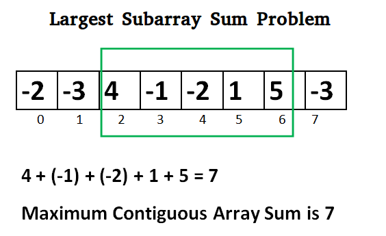
## Example
The list usually contains both positive and negative numbers along
with `0`. For example, for the array of
values `−2, 1, −3, 4, −1, 2, 1, −5, 4` the contiguous subarray
with the largest sum is `4, −1, 2, 1`, with sum `6`.
## Solutions
- Brute Force solution `O(n^2)`: [bfMaximumSubarray.js](./bfMaximumSubarray.js)
- Divide and Conquer solution `O(n^2)`: [dcMaximumSubarraySum.js](./dcMaximumSubarraySum.js)
- Dynamic Programming solution `O(n)`: [dpMaximumSubarray.js](./dpMaximumSubarray.js)
## References
- [Wikipedia](https://en.wikipedia.org/wiki/Maximum_subarray_problem)
- [YouTube](https://www.youtube.com/watch?v=ohHWQf1HDfU&list=PLLXdhg_r2hKA7DPDsunoDZ-Z769jWn4R8)
- [GeeksForGeeks](https://www.geeksforgeeks.org/largest-sum-contiguous-subarray/)
- [LeetCode](https://leetcode.com/explore/interview/card/top-interview-questions-easy/97/dynamic-programming/566/discuss/1595195/C++Python-7-Simple-Solutions-w-Explanation-or-Brute-Force-+-DP-+-Kadane-+-Divide-and-Conquer)
================================================
FILE: src/algorithms/sets/maximum-subarray/__test__/bfMaximumSubarray.test.js
================================================
import bfMaximumSubarray from '../bfMaximumSubarray';
describe('bfMaximumSubarray', () => {
it('should find maximum subarray using the brute force algorithm', () => {
expect(bfMaximumSubarray([])).toEqual([]);
expect(bfMaximumSubarray([0, 0])).toEqual([0]);
expect(bfMaximumSubarray([0, 0, 1])).toEqual([0, 0, 1]);
expect(bfMaximumSubarray([0, 0, 1, 2])).toEqual([0, 0, 1, 2]);
expect(bfMaximumSubarray([0, 0, -1, 2])).toEqual([2]);
expect(bfMaximumSubarray([-1, -2, -3, -4, -5])).toEqual([-1]);
expect(bfMaximumSubarray([1, 2, 3, 2, 3, 4, 5])).toEqual([1, 2, 3, 2, 3, 4, 5]);
expect(bfMaximumSubarray([-2, 1, -3, 4, -1, 2, 1, -5, 4])).toEqual([4, -1, 2, 1]);
expect(bfMaximumSubarray([-2, -3, 4, -1, -2, 1, 5, -3])).toEqual([4, -1, -2, 1, 5]);
expect(bfMaximumSubarray([1, -3, 2, -5, 7, 6, -1, 4, 11, -23])).toEqual([7, 6, -1, 4, 11]);
});
});
================================================
FILE: src/algorithms/sets/maximum-subarray/__test__/dcMaximumSubarraySum.test.js
================================================
import dcMaximumSubarray from '../dcMaximumSubarraySum';
describe('dcMaximumSubarraySum', () => {
it('should find maximum subarray sum using the divide and conquer algorithm', () => {
expect(dcMaximumSubarray([])).toEqual(-Infinity);
expect(dcMaximumSubarray([0, 0])).toEqual(0);
expect(dcMaximumSubarray([0, 0, 1])).toEqual(1);
expect(dcMaximumSubarray([0, 0, 1, 2])).toEqual(3);
expect(dcMaximumSubarray([0, 0, -1, 2])).toEqual(2);
expect(dcMaximumSubarray([-1, -2, -3, -4, -5])).toEqual(-1);
expect(dcMaximumSubarray([1, 2, 3, 2, 3, 4, 5])).toEqual(20);
expect(dcMaximumSubarray([-2, 1, -3, 4, -1, 2, 1, -5, 4])).toEqual(6);
expect(dcMaximumSubarray([-2, -3, 4, -1, -2, 1, 5, -3])).toEqual(7);
expect(dcMaximumSubarray([1, -3, 2, -5, 7, 6, -1, 4, 11, -23])).toEqual(27);
});
});
================================================
FILE: src/algorithms/sets/maximum-subarray/__test__/dpMaximumSubarray.test.js
================================================
import dpMaximumSubarray from '../dpMaximumSubarray';
describe('dpMaximumSubarray', () => {
it('should find maximum subarray using the dynamic programming algorithm', () => {
expect(dpMaximumSubarray([])).toEqual([]);
expect(dpMaximumSubarray([0, 0])).toEqual([0]);
expect(dpMaximumSubarray([0, 0, 1])).toEqual([0, 0, 1]);
expect(dpMaximumSubarray([0, 0, 1, 2])).toEqual([0, 0, 1, 2]);
expect(dpMaximumSubarray([0, 0, -1, 2])).toEqual([2]);
expect(dpMaximumSubarray([-1, -2, -3, -4, -5])).toEqual([-1]);
expect(dpMaximumSubarray([1, 2, 3, 2, 3, 4, 5])).toEqual([1, 2, 3, 2, 3, 4, 5]);
expect(dpMaximumSubarray([-2, 1, -3, 4, -1, 2, 1, -5, 4])).toEqual([4, -1, 2, 1]);
expect(dpMaximumSubarray([-2, -3, 4, -1, -2, 1, 5, -3])).toEqual([4, -1, -2, 1, 5]);
expect(dpMaximumSubarray([1, -3, 2, -5, 7, 6, -1, 4, 11, -23])).toEqual([7, 6, -1, 4, 11]);
});
});
================================================
FILE: src/algorithms/sets/maximum-subarray/bfMaximumSubarray.js
================================================
/**
* Brute Force solution.
* Complexity: O(n^2)
*
* @param {Number[]} inputArray
* @return {Number[]}
*/
export default function bfMaximumSubarray(inputArray) {
let maxSubarrayStartIndex = 0;
let maxSubarrayLength = 0;
let maxSubarraySum = null;
for (let startIndex = 0; startIndex < inputArray.length; startIndex += 1) {
let subarraySum = 0;
for (let arrLength = 1; arrLength <= (inputArray.length - startIndex); arrLength += 1) {
subarraySum += inputArray[startIndex + (arrLength - 1)];
if (maxSubarraySum === null || subarraySum > maxSubarraySum) {
maxSubarraySum = subarraySum;
maxSubarrayStartIndex = startIndex;
maxSubarrayLength = arrLength;
}
}
}
return inputArray.slice(maxSubarrayStartIndex, maxSubarrayStartIndex + maxSubarrayLength);
}
================================================
FILE: src/algorithms/sets/maximum-subarray/dcMaximumSubarraySum.js
================================================
/**
* Divide and Conquer solution.
* Complexity: O(n^2) in case if no memoization applied
*
* @param {Number[]} inputArray
* @return {Number[]}
*/
export default function dcMaximumSubarraySum(inputArray) {
/**
* We are going through the inputArray array and for each element we have two options:
* - to pick
* - not to pick
*
* Also keep in mind, that the maximum sub-array must be contiguous. It means if we picked
* the element, we need to continue picking the next elements or stop counting the max sum.
*
* @param {number} elementIndex - the index of the element we're deciding to pick or not
* @param {boolean} mustPick - to pick or not to pick the element
* @returns {number} - maximum subarray sum that we'll get
*/
function solveRecursively(elementIndex, mustPick) {
if (elementIndex >= inputArray.length) {
return mustPick ? 0 : -Infinity;
}
return Math.max(
// Option #1: Pick the current element, and continue picking next one.
inputArray[elementIndex] + solveRecursively(elementIndex + 1, true),
// Option #2: Don't pick the current element.
mustPick ? 0 : solveRecursively(elementIndex + 1, false),
);
}
return solveRecursively(0, false);
}
================================================
FILE: src/algorithms/sets/maximum-subarray/dpMaximumSubarray.js
================================================
/**
* Dynamic Programming solution.
* Complexity: O(n)
*
* @param {Number[]} inputArray
* @return {Number[]}
*/
export default function dpMaximumSubarray(inputArray) {
// We iterate through the inputArray once, using a greedy approach to keep track of the maximum
// sum we've seen so far and the current sum.
//
// The currentSum variable gets reset to 0 every time it drops below 0.
//
// The maxSum variable is set to -Infinity so that if all numbers are negative, the highest
// negative number will constitute the maximum subarray.
let maxSum = -Infinity;
let currentSum = 0;
// We need to keep track of the starting and ending indices that contributed to our maxSum
// so that we can return the actual subarray. From the beginning let's assume that whole array
// is contributing to maxSum.
let maxStartIndex = 0;
let maxEndIndex = inputArray.length - 1;
let currentStartIndex = 0;
inputArray.forEach((currentNumber, currentIndex) => {
currentSum += currentNumber;
// Update maxSum and the corresponding indices if we have found a new max.
if (maxSum < currentSum) {
maxSum = currentSum;
maxStartIndex = currentStartIndex;
maxEndIndex = currentIndex;
}
// Reset currentSum and currentStartIndex if currentSum drops below 0.
if (currentSum < 0) {
currentSum = 0;
currentStartIndex = currentIndex + 1;
}
});
return inputArray.slice(maxStartIndex, maxEndIndex + 1);
}
================================================
FILE: src/algorithms/sets/permutations/README.md
================================================
# Permutations
When the order doesn't matter, it is a **Combination**.
When the order **does** matter it is a **Permutation**.
**"The combination to the safe is 472"**. We do care about the order. `724` won't work, nor will `247`.
It has to be exactly `4-7-2`.
## Permutations without repetitions
A permutation, also called an “arrangement number” or “order”, is a rearrangement of
the elements of an ordered list `S` into a one-to-one correspondence with `S` itself.
Below are the permutations of string `ABC`.
`ABC ACB BAC BCA CBA CAB`
Or for example the first three people in a running race: you can't be first and second.
**Number of combinations**
```
n * (n-1) * (n -2) * ... * 1 = n!
```
## Permutations with repetitions
When repetition is allowed we have permutations with repetitions.
For example the the lock below: it could be `333`.

**Number of combinations**
```
n * n * n ... (r times) = n^r
```
## Cheatsheet


| | |
| --- | --- |
| |  |
*Made with [okso.app](https://okso.app)*
## References
- [Math Is Fun](https://www.mathsisfun.com/combinatorics/combinations-permutations.html)
- [Permutations/combinations cheat sheets](https://medium.com/@trekhleb/permutations-combinations-algorithms-cheat-sheet-68c14879aba5)
================================================
FILE: src/algorithms/sets/permutations/__test__/permutateWithRepetitions.test.js
================================================
import permutateWithRepetitions from '../permutateWithRepetitions';
describe('permutateWithRepetitions', () => {
it('should permutate string with repetition', () => {
const permutations1 = permutateWithRepetitions(['A']);
expect(permutations1).toEqual([
['A'],
]);
const permutations2 = permutateWithRepetitions(['A', 'B']);
expect(permutations2).toEqual([
['A', 'A'],
['A', 'B'],
['B', 'A'],
['B', 'B'],
]);
const permutations3 = permutateWithRepetitions(['A', 'B', 'C']);
expect(permutations3).toEqual([
['A', 'A', 'A'],
['A', 'A', 'B'],
['A', 'A', 'C'],
['A', 'B', 'A'],
['A', 'B', 'B'],
['A', 'B', 'C'],
['A', 'C', 'A'],
['A', 'C', 'B'],
['A', 'C', 'C'],
['B', 'A', 'A'],
['B', 'A', 'B'],
['B', 'A', 'C'],
['B', 'B', 'A'],
['B', 'B', 'B'],
['B', 'B', 'C'],
['B', 'C', 'A'],
['B', 'C', 'B'],
['B', 'C', 'C'],
['C', 'A', 'A'],
['C', 'A', 'B'],
['C', 'A', 'C'],
['C', 'B', 'A'],
['C', 'B', 'B'],
['C', 'B', 'C'],
['C', 'C', 'A'],
['C', 'C', 'B'],
['C', 'C', 'C'],
]);
const permutations4 = permutateWithRepetitions(['A', 'B', 'C', 'D']);
expect(permutations4.length).toBe(4 * 4 * 4 * 4);
});
});
================================================
FILE: src/algorithms/sets/permutations/__test__/permutateWithoutRepetitions.test.js
================================================
import permutateWithoutRepetitions from '../permutateWithoutRepetitions';
import factorial from '../../../math/factorial/factorial';
describe('permutateWithoutRepetitions', () => {
it('should permutate string', () => {
const permutations1 = permutateWithoutRepetitions(['A']);
expect(permutations1).toEqual([
['A'],
]);
const permutations2 = permutateWithoutRepetitions(['A', 'B']);
expect(permutations2.length).toBe(2);
expect(permutations2).toEqual([
['A', 'B'],
['B', 'A'],
]);
const permutations6 = permutateWithoutRepetitions(['A', 'A']);
expect(permutations6.length).toBe(2);
expect(permutations6).toEqual([
['A', 'A'],
['A', 'A'],
]);
const permutations3 = permutateWithoutRepetitions(['A', 'B', 'C']);
expect(permutations3.length).toBe(factorial(3));
expect(permutations3).toEqual([
['A', 'B', 'C'],
['B', 'A', 'C'],
['B', 'C', 'A'],
['A', 'C', 'B'],
['C', 'A', 'B'],
['C', 'B', 'A'],
]);
const permutations4 = permutateWithoutRepetitions(['A', 'B', 'C', 'D']);
expect(permutations4.length).toBe(factorial(4));
expect(permutations4).toEqual([
['A', 'B', 'C', 'D'],
['B', 'A', 'C', 'D'],
['B', 'C', 'A', 'D'],
['B', 'C', 'D', 'A'],
['A', 'C', 'B', 'D'],
['C', 'A', 'B', 'D'],
['C', 'B', 'A', 'D'],
['C', 'B', 'D', 'A'],
['A', 'C', 'D', 'B'],
['C', 'A', 'D', 'B'],
['C', 'D', 'A', 'B'],
['C', 'D', 'B', 'A'],
['A', 'B', 'D', 'C'],
['B', 'A', 'D', 'C'],
['B', 'D', 'A', 'C'],
['B', 'D', 'C', 'A'],
['A', 'D', 'B', 'C'],
['D', 'A', 'B', 'C'],
['D', 'B', 'A', 'C'],
['D', 'B', 'C', 'A'],
['A', 'D', 'C', 'B'],
['D', 'A', 'C', 'B'],
['D', 'C', 'A', 'B'],
['D', 'C', 'B', 'A'],
]);
const permutations5 = permutateWithoutRepetitions(['A', 'B', 'C', 'D', 'E', 'F']);
expect(permutations5.length).toBe(factorial(6));
});
});
================================================
FILE: src/algorithms/sets/permutations/permutateWithRepetitions.js
================================================
/**
* @param {*[]} permutationOptions
* @param {number} permutationLength
* @return {*[]}
*/
export default function permutateWithRepetitions(
permutationOptions,
permutationLength = permutationOptions.length,
) {
if (permutationLength === 1) {
return permutationOptions.map((permutationOption) => [permutationOption]);
}
// Init permutations array.
const permutations = [];
// Get smaller permutations.
const smallerPermutations = permutateWithRepetitions(
permutationOptions,
permutationLength - 1,
);
// Go through all options and join it to the smaller permutations.
permutationOptions.forEach((currentOption) => {
smallerPermutations.forEach((smallerPermutation) => {
permutations.push([currentOption].concat(smallerPermutation));
});
});
return permutations;
}
================================================
FILE: src/algorithms/sets/permutations/permutateWithoutRepetitions.js
================================================
/**
* @param {*[]} permutationOptions
* @return {*[]}
*/
export default function permutateWithoutRepetitions(permutationOptions) {
if (permutationOptions.length === 1) {
return [permutationOptions];
}
// Init permutations array.
const permutations = [];
// Get all permutations for permutationOptions excluding the first element.
const smallerPermutations = permutateWithoutRepetitions(permutationOptions.slice(1));
// Insert first option into every possible position of every smaller permutation.
const firstOption = permutationOptions[0];
for (let permIndex = 0; permIndex < smallerPermutations.length; permIndex += 1) {
const smallerPermutation = smallerPermutations[permIndex];
// Insert first option into every possible position of smallerPermutation.
for (let positionIndex = 0; positionIndex <= smallerPermutation.length; positionIndex += 1) {
const permutationPrefix = smallerPermutation.slice(0, positionIndex);
const permutationSuffix = smallerPermutation.slice(positionIndex);
permutations.push(permutationPrefix.concat([firstOption], permutationSuffix));
}
}
return permutations;
}
================================================
FILE: src/algorithms/sets/power-set/README.md
================================================
# Power Set
Power set of a set `S` is the set of all of the subsets of `S`, including the
empty set and `S` itself. Power set of set `S` is denoted as `P(S)`.
For example for `{x, y, z}`, the subsets
are:
```text
{
{}, // (also denoted empty set ∅ or the null set)
{x},
{y},
{z},
{x, y},
{x, z},
{y, z},
{x, y, z}
}
```

Here is how we may illustrate the elements of the power set of the set `{x, y, z}` ordered with respect to
inclusion:

**Number of Subsets**
If `S` is a finite set with `|S| = n` elements, then the number of subsets
of `S` is `|P(S)| = 2^n`. This fact, which is the motivation for the
notation `2^S`, may be demonstrated simply as follows:
> First, order the elements of `S` in any manner. We write any subset of `S` in
the format `{γ1, γ2, ..., γn}` where `γi , 1 ≤ i ≤ n`, can take the value
of `0` or `1`. If `γi = 1`, the `i`-th element of `S` is in the subset;
otherwise, the `i`-th element is not in the subset. Clearly the number of
distinct subsets that can be constructed this way is `2^n` as `γi ∈ {0, 1}`.
## Algorithms
### Bitwise Solution
Each number in binary representation in a range from `0` to `2^n` does exactly
what we need: it shows by its bits (`0` or `1`) whether to include related
element from the set or not. For example, for the set `{1, 2, 3}` the binary
number of `0b010` would mean that we need to include only `2` to the current set.
| | `abc` | Subset |
| :---: | :---: | :-----------: |
| `0` | `000` | `{}` |
| `1` | `001` | `{c}` |
| `2` | `010` | `{b}` |
| `3` | `011` | `{c, b}` |
| `4` | `100` | `{a}` |
| `5` | `101` | `{a, c}` |
| `6` | `110` | `{a, b}` |
| `7` | `111` | `{a, b, c}` |
> See [bwPowerSet.js](./bwPowerSet.js) file for bitwise solution.
### Backtracking Solution
In backtracking approach we're constantly trying to add next element of the set
to the subset, memorizing it and then removing it and try the same with the next
element.
> See [btPowerSet.js](./btPowerSet.js) file for backtracking solution.
### Cascading Solution
This is, arguably, the simplest solution to generate a Power Set.
We start with an empty set:
```text
powerSets = [[]]
```
Now, let's say:
```text
originalSet = [1, 2, 3]
```
Let's add the 1st element from the originalSet to all existing sets:
```text
[[]] ← 1 = [[], [1]]
```
Adding the 2nd element to all existing sets:
```text
[[], [1]] ← 2 = [[], [1], [2], [1, 2]]
```
Adding the 3nd element to all existing sets:
```
[[], [1], [2], [1, 2]] ← 3 = [[], [1], [2], [1, 2], [3], [1, 3], [2, 3], [1, 2, 3]]
```
And so on, for the rest of the elements from the `originalSet`. On every iteration the number of sets is doubled, so we'll get `2^n` sets.
> See [caPowerSet.js](./caPowerSet.js) file for cascading solution.
## References
* [Wikipedia](https://en.wikipedia.org/wiki/Power_set)
* [Math is Fun](https://www.mathsisfun.com/sets/power-set.html)
================================================
FILE: src/algorithms/sets/power-set/__test__/btPowerSet.test.js
================================================
import btPowerSet from '../btPowerSet';
describe('btPowerSet', () => {
it('should calculate power set of given set using backtracking approach', () => {
expect(btPowerSet([1])).toEqual([
[],
[1],
]);
expect(btPowerSet([1, 2, 3])).toEqual([
[],
[1],
[1, 2],
[1, 2, 3],
[1, 3],
[2],
[2, 3],
[3],
]);
});
});
================================================
FILE: src/algorithms/sets/power-set/__test__/bwPowerSet.test.js
================================================
import bwPowerSet from '../bwPowerSet';
describe('bwPowerSet', () => {
it('should calculate power set of given set using bitwise approach', () => {
expect(bwPowerSet([1])).toEqual([
[],
[1],
]);
expect(bwPowerSet([1, 2, 3])).toEqual([
[],
[1],
[2],
[1, 2],
[3],
[1, 3],
[2, 3],
[1, 2, 3],
]);
});
});
================================================
FILE: src/algorithms/sets/power-set/__test__/caPowerSet.test.js
================================================
import caPowerSet from '../caPowerSet';
describe('caPowerSet', () => {
it('should calculate power set of given set using cascading approach', () => {
expect(caPowerSet([1])).toEqual([
[],
[1],
]);
expect(caPowerSet([1, 2])).toEqual([
[],
[1],
[2],
[1, 2],
]);
expect(caPowerSet([1, 2, 3])).toEqual([
[],
[1],
[2],
[1, 2],
[3],
[1, 3],
[2, 3],
[1, 2, 3],
]);
});
});
================================================
FILE: src/algorithms/sets/power-set/btPowerSet.js
================================================
/**
* @param {*[]} originalSet - Original set of elements we're forming power-set of.
* @param {*[][]} allSubsets - All subsets that have been formed so far.
* @param {*[]} currentSubSet - Current subset that we're forming at the moment.
* @param {number} startAt - The position of in original set we're starting to form current subset.
* @return {*[][]} - All subsets of original set.
*/
function btPowerSetRecursive(originalSet, allSubsets = [[]], currentSubSet = [], startAt = 0) {
// Let's iterate over originalSet elements that may be added to the subset
// without having duplicates. The value of startAt prevents adding the duplicates.
for (let position = startAt; position < originalSet.length; position += 1) {
// Let's push current element to the subset
currentSubSet.push(originalSet[position]);
// Current subset is already valid so let's memorize it.
// We do array destruction here to save the clone of the currentSubSet.
// We need to save a clone since the original currentSubSet is going to be
// mutated in further recursive calls.
allSubsets.push([...currentSubSet]);
// Let's try to generate all other subsets for the current subset.
// We're increasing the position by one to avoid duplicates in subset.
btPowerSetRecursive(originalSet, allSubsets, currentSubSet, position + 1);
// BACKTRACK. Exclude last element from the subset and try the next valid one.
currentSubSet.pop();
}
// Return all subsets of a set.
return allSubsets;
}
/**
* Find power-set of a set using BACKTRACKING approach.
*
* @param {*[]} originalSet
* @return {*[][]}
*/
export default function btPowerSet(originalSet) {
return btPowerSetRecursive(originalSet);
}
================================================
FILE: src/algorithms/sets/power-set/bwPowerSet.js
================================================
/**
* Find power-set of a set using BITWISE approach.
*
* @param {*[]} originalSet
* @return {*[][]}
*/
export default function bwPowerSet(originalSet) {
const subSets = [];
// We will have 2^n possible combinations (where n is a length of original set).
// It is because for every element of original set we will decide whether to include
// it or not (2 options for each set element).
const numberOfCombinations = 2 ** originalSet.length;
// Each number in binary representation in a range from 0 to 2^n does exactly what we need:
// it shows by its bits (0 or 1) whether to include related element from the set or not.
// For example, for the set {1, 2, 3} the binary number of 0b010 would mean that we need to
// include only "2" to the current set.
for (let combinationIndex = 0; combinationIndex < numberOfCombinations; combinationIndex += 1) {
const subSet = [];
for (let setElementIndex = 0; setElementIndex < originalSet.length; setElementIndex += 1) {
// Decide whether we need to include current element into the subset or not.
if (combinationIndex & (1 << setElementIndex)) {
subSet.push(originalSet[setElementIndex]);
}
}
// Add current subset to the list of all subsets.
subSets.push(subSet);
}
return subSets;
}
================================================
FILE: src/algorithms/sets/power-set/caPowerSet.js
================================================
/**
* Find power-set of a set using CASCADING approach.
*
* @param {*[]} originalSet
* @return {*[][]}
*/
export default function caPowerSet(originalSet) {
// Let's start with an empty set.
const sets = [[]];
/*
Now, let's say:
originalSet = [1, 2, 3].
Let's add the first element from the originalSet to all existing sets:
[[]] ← 1 = [[], [1]]
Adding the 2nd element to all existing sets:
[[], [1]] ← 2 = [[], [1], [2], [1, 2]]
Adding the 3nd element to all existing sets:
[[], [1], [2], [1, 2]] ← 3 = [[], [1], [2], [1, 2], [3], [1, 3], [2, 3], [1, 2, 3]]
And so on for the rest of the elements from originalSet.
On every iteration the number of sets is doubled, so we'll get 2^n sets.
*/
for (let numIdx = 0; numIdx < originalSet.length; numIdx += 1) {
const existingSetsNum = sets.length;
for (let setIdx = 0; setIdx < existingSetsNum; setIdx += 1) {
const set = [...sets[setIdx], originalSet[numIdx]];
sets.push(set);
}
}
return sets;
}
================================================
FILE: src/algorithms/sets/shortest-common-supersequence/README.md
================================================
# Shortest Common Supersequence
The shortest common supersequence (SCS) of two sequences `X` and `Y`
is the shortest sequence which has `X` and `Y` as subsequences.
In other words assume we're given two strings str1 and str2, find
the shortest string that has both str1 and str2 as subsequences.
This is a problem closely related to the longest common
subsequence problem.
## Example
```
Input: str1 = "geek", str2 = "eke"
Output: "geeke"
Input: str1 = "AGGTAB", str2 = "GXTXAYB"
Output: "AGXGTXAYB"
```
## References
- [GeeksForGeeks](https://www.geeksforgeeks.org/shortest-common-supersequence/)
================================================
FILE: src/algorithms/sets/shortest-common-supersequence/__test__/shortestCommonSupersequence.test.js
================================================
import shortestCommonSupersequence from '../shortestCommonSupersequence';
describe('shortestCommonSupersequence', () => {
it('should find shortest common supersequence of two sequences', () => {
// LCS (longest common subsequence) is empty
expect(shortestCommonSupersequence(
['A', 'B', 'C'],
['D', 'E', 'F'],
)).toEqual(['A', 'B', 'C', 'D', 'E', 'F']);
// LCS (longest common subsequence) is "EE"
expect(shortestCommonSupersequence(
['G', 'E', 'E', 'K'],
['E', 'K', 'E'],
)).toEqual(['G', 'E', 'K', 'E', 'K']);
// LCS (longest common subsequence) is "GTAB"
expect(shortestCommonSupersequence(
['A', 'G', 'G', 'T', 'A', 'B'],
['G', 'X', 'T', 'X', 'A', 'Y', 'B'],
)).toEqual(['A', 'G', 'G', 'X', 'T', 'X', 'A', 'Y', 'B']);
// LCS (longest common subsequence) is "BCBA".
expect(shortestCommonSupersequence(
['A', 'B', 'C', 'B', 'D', 'A', 'B'],
['B', 'D', 'C', 'A', 'B', 'A'],
)).toEqual(['A', 'B', 'D', 'C', 'A', 'B', 'D', 'A', 'B']);
// LCS (longest common subsequence) is "BDABA".
expect(shortestCommonSupersequence(
['B', 'D', 'C', 'A', 'B', 'A'],
['A', 'B', 'C', 'B', 'D', 'A', 'B', 'A', 'C'],
)).toEqual(['A', 'B', 'C', 'B', 'D', 'C', 'A', 'B', 'A', 'C']);
});
});
================================================
FILE: src/algorithms/sets/shortest-common-supersequence/shortestCommonSupersequence.js
================================================
import longestCommonSubsequence from '../longest-common-subsequence/longestCommonSubsequence';
/**
* @param {string[]} set1
* @param {string[]} set2
* @return {string[]}
*/
export default function shortestCommonSupersequence(set1, set2) {
// Let's first find the longest common subsequence of two sets.
const lcs = longestCommonSubsequence(set1, set2);
// If LCS is empty then the shortest common supersequence would be just
// concatenation of two sequences.
if (lcs.length === 1 && lcs[0] === '') {
return set1.concat(set2);
}
// Now let's add elements of set1 and set2 in order before/inside/after the LCS.
let supersequence = [];
let setIndex1 = 0;
let setIndex2 = 0;
let lcsIndex = 0;
let setOnHold1 = false;
let setOnHold2 = false;
while (lcsIndex < lcs.length) {
// Add elements of the first set to supersequence in correct order.
if (setIndex1 < set1.length) {
if (!setOnHold1 && set1[setIndex1] !== lcs[lcsIndex]) {
supersequence.push(set1[setIndex1]);
setIndex1 += 1;
} else {
setOnHold1 = true;
}
}
// Add elements of the second set to supersequence in correct order.
if (setIndex2 < set2.length) {
if (!setOnHold2 && set2[setIndex2] !== lcs[lcsIndex]) {
supersequence.push(set2[setIndex2]);
setIndex2 += 1;
} else {
setOnHold2 = true;
}
}
// Add LCS element to the supersequence in correct order.
if (setOnHold1 && setOnHold2) {
supersequence.push(lcs[lcsIndex]);
lcsIndex += 1;
setIndex1 += 1;
setIndex2 += 1;
setOnHold1 = false;
setOnHold2 = false;
}
}
// Attach set1 leftovers.
if (setIndex1 < set1.length) {
supersequence = supersequence.concat(set1.slice(setIndex1));
}
// Attach set2 leftovers.
if (setIndex2 < set2.length) {
supersequence = supersequence.concat(set2.slice(setIndex2));
}
return supersequence;
}
================================================
FILE: src/algorithms/sorting/Sort.js
================================================
import Comparator from '../../utils/comparator/Comparator';
/**
* @typedef {Object} SorterCallbacks
* @property {function(a: *, b: *)} compareCallback - If provided then all elements comparisons
* will be done through this callback.
* @property {function(a: *)} visitingCallback - If provided it will be called each time the sorting
* function is visiting the next element.
*/
export default class Sort {
constructor(originalCallbacks) {
this.callbacks = Sort.initSortingCallbacks(originalCallbacks);
this.comparator = new Comparator(this.callbacks.compareCallback);
}
/**
* @param {SorterCallbacks} originalCallbacks
* @returns {SorterCallbacks}
*/
static initSortingCallbacks(originalCallbacks) {
const callbacks = originalCallbacks || {};
const stubCallback = () => {};
callbacks.compareCallback = callbacks.compareCallback || undefined;
callbacks.visitingCallback = callbacks.visitingCallback || stubCallback;
return callbacks;
}
sort() {
throw new Error('sort method must be implemented');
}
}
================================================
FILE: src/algorithms/sorting/SortTester.js
================================================
export const sortedArr = [1, 2, 3, 4, 5, 6, 7, 8, 9, 10, 11, 12, 13, 14, 15, 16, 17, 18, 19, 20];
export const reverseArr = [20, 19, 18, 17, 16, 15, 14, 13, 12, 11, 10, 9, 8, 7, 6, 5, 4, 3, 2, 1];
export const notSortedArr = [15, 8, 5, 12, 10, 1, 16, 9, 11, 7, 20, 3, 2, 6, 17, 18, 4, 13, 14, 19];
export const equalArr = [1, 1, 1, 1, 1, 1, 1, 1, 1, 1, 1, 1, 1, 1, 1, 1, 1, 1, 1, 1];
export const negativeArr = [-1, 0, 5, -10, 20, 13, -7, 3, 2, -3];
export const negativeArrSorted = [-10, -7, -3, -1, 0, 2, 3, 5, 13, 20];
export class SortTester {
static testSort(SortingClass) {
const sorter = new SortingClass();
expect(sorter.sort([])).toEqual([]);
expect(sorter.sort([1])).toEqual([1]);
expect(sorter.sort([1, 2])).toEqual([1, 2]);
expect(sorter.sort([2, 1])).toEqual([1, 2]);
expect(sorter.sort([3, 4, 2, 1, 0, 0, 4, 3, 4, 2])).toEqual([0, 0, 1, 2, 2, 3, 3, 4, 4, 4]);
expect(sorter.sort(sortedArr)).toEqual(sortedArr);
expect(sorter.sort(reverseArr)).toEqual(sortedArr);
expect(sorter.sort(notSortedArr)).toEqual(sortedArr);
expect(sorter.sort(equalArr)).toEqual(equalArr);
}
static testNegativeNumbersSort(SortingClass) {
const sorter = new SortingClass();
expect(sorter.sort(negativeArr)).toEqual(negativeArrSorted);
}
static testSortWithCustomComparator(SortingClass) {
const callbacks = {
compareCallback: (a, b) => {
if (a.length === b.length) {
return 0;
}
return a.length < b.length ? -1 : 1;
},
};
const sorter = new SortingClass(callbacks);
expect(sorter.sort([''])).toEqual(['']);
expect(sorter.sort(['a'])).toEqual(['a']);
expect(sorter.sort(['aa', 'a'])).toEqual(['a', 'aa']);
expect(sorter.sort(['aa', 'q', 'bbbb', 'ccc'])).toEqual(['q', 'aa', 'ccc', 'bbbb']);
expect(sorter.sort(['aa', 'aa'])).toEqual(['aa', 'aa']);
}
static testSortStability(SortingClass) {
const callbacks = {
compareCallback: (a, b) => {
if (a.length === b.length) {
return 0;
}
return a.length < b.length ? -1 : 1;
},
};
const sorter = new SortingClass(callbacks);
expect(sorter.sort(['bb', 'aa', 'c'])).toEqual(['c', 'bb', 'aa']);
expect(sorter.sort(['aa', 'q', 'a', 'bbbb', 'ccc'])).toEqual(['q', 'a', 'aa', 'ccc', 'bbbb']);
}
static testAlgorithmTimeComplexity(SortingClass, arrayToBeSorted, numberOfVisits) {
const visitingCallback = jest.fn();
const callbacks = { visitingCallback };
const sorter = new SortingClass(callbacks);
sorter.sort(arrayToBeSorted);
expect(visitingCallback).toHaveBeenCalledTimes(numberOfVisits);
}
}
================================================
FILE: src/algorithms/sorting/__test__/Sort.test.js
================================================
import Sort from '../Sort';
describe('Sort', () => {
it('should throw an error when trying to call Sort.sort() method directly', () => {
function doForbiddenSort() {
const sorter = new Sort();
sorter.sort();
}
expect(doForbiddenSort).toThrow();
});
});
================================================
FILE: src/algorithms/sorting/bubble-sort/BubbleSort.js
================================================
import Sort from '../Sort';
export default class BubbleSort extends Sort {
sort(originalArray) {
// Flag that holds info about whether the swap has occur or not.
let swapped = false;
// Clone original array to prevent its modification.
const array = [...originalArray];
for (let i = 1; i < array.length; i += 1) {
swapped = false;
// Call visiting callback.
this.callbacks.visitingCallback(array[i]);
for (let j = 0; j < array.length - i; j += 1) {
// Call visiting callback.
this.callbacks.visitingCallback(array[j]);
// Swap elements if they are in wrong order.
if (this.comparator.lessThan(array[j + 1], array[j])) {
[array[j], array[j + 1]] = [array[j + 1], array[j]];
// Register the swap.
swapped = true;
}
}
// If there were no swaps then array is already sorted and there is
// no need to proceed.
if (!swapped) {
return array;
}
}
return array;
}
}
================================================
FILE: src/algorithms/sorting/bubble-sort/README.md
================================================
# Bubble Sort
_Read this in other languages:_
[_Português_](README.pt-BR.md)
Bubble sort, sometimes referred to as sinking sort, is a
simple sorting algorithm that repeatedly steps through
the list to be sorted, compares each pair of adjacent
items and swaps them if they are in the wrong order
(ascending or descending arrangement). The pass through
the list is repeated until no swaps are needed, which
indicates that the list is sorted.

## Complexity
| Name | Best | Average | Worst | Memory | Stable | Comments |
| --------------------- | :-------------: | :-----------------: | :-----------------: | :-------: | :-------: | :-------- |
| **Bubble sort** | n | n2 | n2 | 1 | Yes | |
## References
- [Wikipedia](https://en.wikipedia.org/wiki/Bubble_sort)
- [YouTube](https://www.youtube.com/watch?v=6Gv8vg0kcHc&index=27&t=0s&list=PLLXdhg_r2hKA7DPDsunoDZ-Z769jWn4R8)
================================================
FILE: src/algorithms/sorting/bubble-sort/README.pt-BR.md
================================================
# Bubble Sort
_Leia isso em outros idiomas:_
[_English_](README.md)
O bubble sort, ou ordenação por flutuação (literalmente "por bolha"), é um algoritmo de ordenação dos mais simples. A ideia é percorrer o vetor diversas vezes, e a cada passagem fazer flutuar para o topo o maior elemento da sequência. Essa movimentação lembra a forma como as bolhas em um tanque de água procuram seu próprio nível, e disso vem o nome do algoritmo.

## Complexidade
| Nome | Melhor | Média | Pior | Memória | Estável | Comentários |
| --------------------- | :-------------: | :-----------------: | :-----------------: | :-------: | :-------: | :-------- |
| **Bubble sort** | n | n2 | n2 | 1 | Sim | |
## Referências
- [Wikipedia](https://pt.wikipedia.org/wiki/Bubble_sort)
- [YouTube](https://www.youtube.com/watch?v=6Gv8vg0kcHc&index=27&t=0s&list=PLLXdhg_r2hKA7DPDsunoDZ-Z769jWn4R8)
================================================
FILE: src/algorithms/sorting/bubble-sort/__test__/BubbleSort.test.js
================================================
import BubbleSort from '../BubbleSort';
import {
equalArr,
notSortedArr,
reverseArr,
sortedArr,
SortTester,
} from '../../SortTester';
// Complexity constants.
const SORTED_ARRAY_VISITING_COUNT = 20;
const NOT_SORTED_ARRAY_VISITING_COUNT = 189;
const REVERSE_SORTED_ARRAY_VISITING_COUNT = 209;
const EQUAL_ARRAY_VISITING_COUNT = 20;
describe('BubbleSort', () => {
it('should sort array', () => {
SortTester.testSort(BubbleSort);
});
it('should sort array with custom comparator', () => {
SortTester.testSortWithCustomComparator(BubbleSort);
});
it('should do stable sorting', () => {
SortTester.testSortStability(BubbleSort);
});
it('should sort negative numbers', () => {
SortTester.testNegativeNumbersSort(BubbleSort);
});
it('should visit EQUAL array element specified number of times', () => {
SortTester.testAlgorithmTimeComplexity(
BubbleSort,
equalArr,
EQUAL_ARRAY_VISITING_COUNT,
);
});
it('should visit SORTED array element specified number of times', () => {
SortTester.testAlgorithmTimeComplexity(
BubbleSort,
sortedArr,
SORTED_ARRAY_VISITING_COUNT,
);
});
it('should visit NOT SORTED array element specified number of times', () => {
SortTester.testAlgorithmTimeComplexity(
BubbleSort,
notSortedArr,
NOT_SORTED_ARRAY_VISITING_COUNT,
);
});
it('should visit REVERSE SORTED array element specified number of times', () => {
SortTester.testAlgorithmTimeComplexity(
BubbleSort,
reverseArr,
REVERSE_SORTED_ARRAY_VISITING_COUNT,
);
});
});
================================================
FILE: src/algorithms/sorting/bucket-sort/BucketSort.js
================================================
import RadixSort from '../radix-sort/RadixSort';
/**
* Bucket Sort
*
* @param {number[]} arr
* @param {number} bucketsNum
* @return {number[]}
*/
export default function BucketSort(arr, bucketsNum = 1) {
const buckets = new Array(bucketsNum).fill(null).map(() => []);
const minValue = Math.min(...arr);
const maxValue = Math.max(...arr);
const bucketSize = Math.ceil(Math.max(1, (maxValue - minValue) / bucketsNum));
// Place elements into buckets.
for (let i = 0; i < arr.length; i += 1) {
const currValue = arr[i];
const bucketIndex = Math.floor((currValue - minValue) / bucketSize);
// Edge case for max value.
if (bucketIndex === bucketsNum) {
buckets[bucketsNum - 1].push(currValue);
} else {
buckets[bucketIndex].push(currValue);
}
}
// Sort individual buckets.
for (let i = 0; i < buckets.length; i += 1) {
// Let's use the Radix Sorter here. This may give us
// the average O(n + k) time complexity to sort one bucket
// (where k is a number of digits in the longest number).
buckets[i] = new RadixSort().sort(buckets[i]);
}
// Merge sorted buckets into final output.
const sortedArr = [];
for (let i = 0; i < buckets.length; i += 1) {
sortedArr.push(...buckets[i]);
}
return sortedArr;
}
================================================
FILE: src/algorithms/sorting/bucket-sort/README.md
================================================
# Bucket Sort
**Bucket sort**, or **bin sort**, is a sorting algorithm that works by distributing the elements of an array into a number of buckets. Each bucket is then sorted individually, either using a different sorting algorithm, or by recursively applying the bucket sorting algorithm.
## Algorithm
Bucket sort works as follows:
1. Set up an array of initially empty `buckets`.
2. **Scatter:** Go over the original array, putting each object in its `bucket`.
3. Sort each non-empty `bucket`.
4. **Gather:** Visit the `buckets` in order and put all elements back into the original array.
Elements are distributed among bins:

Then, elements are sorted within each bin:

## Complexity
The computational complexity depends on the algorithm used to sort each bucket, the number of buckets to use, and whether the input is uniformly distributed.
The **worst-case** time complexity of bucket sort is
`O(n^2)` if the sorting algorithm used on the bucket is *insertion sort*, which is the most common use case since the expectation is that buckets will not have too many elements relative to the entire list. In the worst case, all elements are placed in one bucket, causing the running time to reduce to the worst-case complexity of insertion sort (all elements are in reverse order). If the worst-case running time of the intermediate sort used is `O(n * log(n))`, then the worst-case running time of bucket sort will also be
`O(n * log(n))`.
On **average**, when the distribution of elements across buckets is reasonably uniform, it can be shown that bucket sort runs on average `O(n + k)` for `k` buckets.
## References
- [Bucket Sort on Wikipedia](https://en.wikipedia.org/wiki/Bucket_sort)
================================================
FILE: src/algorithms/sorting/bucket-sort/__test__/BucketSort.test.js
================================================
import BucketSort from '../BucketSort';
import {
equalArr,
notSortedArr,
reverseArr,
sortedArr,
} from '../../SortTester';
describe('BucketSort', () => {
it('should sort the array of numbers with different buckets amounts', () => {
expect(BucketSort(notSortedArr, 4)).toEqual(sortedArr);
expect(BucketSort(equalArr, 4)).toEqual(equalArr);
expect(BucketSort(reverseArr, 4)).toEqual(sortedArr);
expect(BucketSort(sortedArr, 4)).toEqual(sortedArr);
expect(BucketSort(notSortedArr, 10)).toEqual(sortedArr);
expect(BucketSort(equalArr, 10)).toEqual(equalArr);
expect(BucketSort(reverseArr, 10)).toEqual(sortedArr);
expect(BucketSort(sortedArr, 10)).toEqual(sortedArr);
expect(BucketSort(notSortedArr, 50)).toEqual(sortedArr);
expect(BucketSort(equalArr, 50)).toEqual(equalArr);
expect(BucketSort(reverseArr, 50)).toEqual(sortedArr);
expect(BucketSort(sortedArr, 50)).toEqual(sortedArr);
});
it('should sort the array of numbers with the default buckets of 1', () => {
expect(BucketSort(notSortedArr)).toEqual(sortedArr);
expect(BucketSort(equalArr)).toEqual(equalArr);
expect(BucketSort(reverseArr)).toEqual(sortedArr);
expect(BucketSort(sortedArr)).toEqual(sortedArr);
});
});
================================================
FILE: src/algorithms/sorting/counting-sort/CountingSort.js
================================================
import Sort from '../Sort';
export default class CountingSort extends Sort {
/**
* @param {number[]} originalArray
* @param {number} [smallestElement]
* @param {number} [biggestElement]
*/
sort(originalArray, smallestElement = undefined, biggestElement = undefined) {
// Init biggest and smallest elements in array in order to build number bucket array later.
let detectedSmallestElement = smallestElement || 0;
let detectedBiggestElement = biggestElement || 0;
if (smallestElement === undefined || biggestElement === undefined) {
originalArray.forEach((element) => {
// Visit element.
this.callbacks.visitingCallback(element);
// Detect biggest element.
if (this.comparator.greaterThan(element, detectedBiggestElement)) {
detectedBiggestElement = element;
}
// Detect smallest element.
if (this.comparator.lessThan(element, detectedSmallestElement)) {
detectedSmallestElement = element;
}
});
}
// Init buckets array.
// This array will hold frequency of each number from originalArray.
const buckets = Array(detectedBiggestElement - detectedSmallestElement + 1).fill(0);
originalArray.forEach((element) => {
// Visit element.
this.callbacks.visitingCallback(element);
buckets[element - detectedSmallestElement] += 1;
});
// Add previous frequencies to the current one for each number in bucket
// to detect how many numbers less then current one should be standing to
// the left of current one.
for (let bucketIndex = 1; bucketIndex < buckets.length; bucketIndex += 1) {
buckets[bucketIndex] += buckets[bucketIndex - 1];
}
// Now let's shift frequencies to the right so that they show correct numbers.
// I.e. if we won't shift right than the value of buckets[5] will display how many
// elements less than 5 should be placed to the left of 5 in sorted array
// INCLUDING 5th. After shifting though this number will not include 5th anymore.
buckets.pop();
buckets.unshift(0);
// Now let's assemble sorted array.
const sortedArray = Array(originalArray.length).fill(null);
for (let elementIndex = 0; elementIndex < originalArray.length; elementIndex += 1) {
// Get the element that we want to put into correct sorted position.
const element = originalArray[elementIndex];
// Visit element.
this.callbacks.visitingCallback(element);
// Get correct position of this element in sorted array.
const elementSortedPosition = buckets[element - detectedSmallestElement];
// Put element into correct position in sorted array.
sortedArray[elementSortedPosition] = element;
// Increase position of current element in the bucket for future correct placements.
buckets[element - detectedSmallestElement] += 1;
}
// Return sorted array.
return sortedArray;
}
}
================================================
FILE: src/algorithms/sorting/counting-sort/README.md
================================================
# Counting Sort
_Read this in other languages:_
[_Português_](README.pt-BR.md)
In computer science, **counting sort** is an algorithm for sorting
a collection of objects according to keys that are small integers;
that is, it is an integer sorting algorithm. It operates by
counting the number of objects that have each distinct key value,
and using arithmetic on those counts to determine the positions
of each key value in the output sequence. Its running time is
linear in the number of items and the difference between the
maximum and minimum key values, so it is only suitable for direct
use in situations where the variation in keys is not significantly
greater than the number of items. However, it is often used as a
subroutine in another sorting algorithm, radix sort, that can
handle larger keys more efficiently.
Because counting sort uses key values as indexes into an array,
it is not a comparison sort, and the `Ω(n log n)` lower bound for
comparison sorting does not apply to it. Bucket sort may be used
for many of the same tasks as counting sort, with a similar time
analysis; however, compared to counting sort, bucket sort requires
linked lists, dynamic arrays or a large amount of preallocated
memory to hold the sets of items within each bucket, whereas
counting sort instead stores a single number (the count of items)
per bucket.
Counting sorting works best when the range of numbers for each array
element is very small.
## Algorithm
**Step I**
In first step we calculate the count of all the elements of the
input array `A`. Then Store the result in the count array `C`.
The way we count is depicted below.
**Step II**
In second step we calculate how many elements exist in the input
array `A` which are less than or equals for the given index.
`Ci` = numbers of elements less than or equals to `i` in input array.
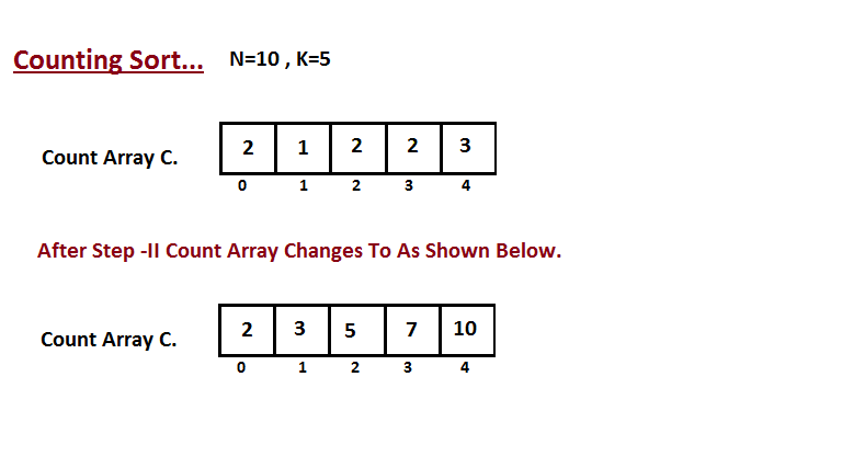
**Step III**
In this step we place the input array `A` element at sorted
position by taking help of constructed count array `C` ,i.e what
we constructed in step two. We used the result array `B` to store
the sorted elements. Here we handled the index of `B` start from
zero.
## Complexity
| Name | Best | Average | Worst | Memory | Stable | Comments |
| --------------------- | :-------------: | :-----------------: | :-----------------: | :-------: | :-------: | :-------- |
| **Counting sort** | n + r | n + r | n + r | n + r | Yes | r - biggest number in array |
## References
- [Wikipedia](https://en.wikipedia.org/wiki/Counting_sort)
- [YouTube](https://www.youtube.com/watch?v=OKd534EWcdk&index=61&t=0s&list=PLLXdhg_r2hKA7DPDsunoDZ-Z769jWn4R8)
- [EfficientAlgorithms](https://efficientalgorithms.blogspot.com/2016/09/lenear-sorting-counting-sort.html)
================================================
FILE: src/algorithms/sorting/counting-sort/README.pt-br.md
================================================
# Counting Sort
_Leia isso em outros idiomas:_
[_English_](README.md)
Em ciência da computação, **counting sort** é um algoritmo para ordenar
uma coleção de objetos de acordo com chaves que são pequenos inteiros;
ou seja, é um algoritmo de ordenação de inteiros. Ele opera por
contando o número de objetos que têm cada valor de chave distinto,
e usando aritmética nessas contagens para determinar as posições
de cada valor de chave na sequência de saída. Seu tempo de execução é
linear no número de itens e a diferença entre o
valores de chave máximo e mínimo, portanto, é adequado apenas para
uso em situações em que a variação de tonalidades não é significativamente
maior que o número de itens. No entanto, muitas vezes é usado como
sub-rotina em outro algoritmo de ordenação, radix sort, que pode
lidar com chaves maiores de forma mais eficiente.
Como a classificação por contagem usa valores-chave como índices em um vetor,
não é uma ordenação por comparação, e o limite inferior `Ω(n log n)` para
a ordenação por comparação não se aplica a ele. A classificação por bucket pode ser usada
para muitas das mesmas tarefas que a ordenação por contagem, com um tempo semelhante
análise; no entanto, em comparação com a classificação por contagem, a classificação por bucket requer
listas vinculadas, arrays dinâmicos ou uma grande quantidade de pré-alocados
memória para armazenar os conjuntos de itens dentro de cada bucket, enquanto
A classificação por contagem armazena um único número (a contagem de itens)
por balde.
A classificação por contagem funciona melhor quando o intervalo de números para cada
elemento do vetor é muito pequeno.
## Algoritmo
**Passo I**
Na primeira etapa, calculamos a contagem de todos os elementos do
vetor de entrada 'A'. Em seguida, armazene o resultado no vetor de contagem `C`.
A maneira como contamos é descrita abaixo.

**Passo II**
Na segunda etapa, calculamos quantos elementos existem na entrada
do vetor `A` que são menores ou iguais para o índice fornecido.
`Ci` = números de elementos menores ou iguais a `i` no vetor de entrada.

**Passo III**
Nesta etapa, colocamos o elemento `A` do vetor de entrada em classificado
posição usando a ajuda do vetor de contagem construída `C`, ou seja, o que
construímos no passo dois. Usamos o vetor de resultados `B` para armazenar
os elementos ordenados. Aqui nós lidamos com o índice de `B` começando de
zero.

## Complexidade
| Nome | Melhor | Média | Pior | Memória | Estável | Comentários |
| --------------------- | :-------------: | :-----------------: | :-----------------: | :-------: | :-------: | :-------- |
| **Counting sort** | n + r | n + r | n + r | n + r | Sim | r - Maior número no vetor |
## Referências
- [Wikipedia](https://en.wikipedia.org/wiki/Counting_sort)
- [YouTube](https://www.youtube.com/watch?v=OKd534EWcdk&index=61&t=0s&list=PLLXdhg_r2hKA7DPDsunoDZ-Z769jWn4R8)
- [EfficientAlgorithms](https://efficientalgorithms.blogspot.com/2016/09/lenear-sorting-counting-sort.html)
================================================
FILE: src/algorithms/sorting/counting-sort/__test__/CountingSort.test.js
================================================
import CountingSort from '../CountingSort';
import {
equalArr,
notSortedArr,
reverseArr,
sortedArr,
SortTester,
} from '../../SortTester';
// Complexity constants.
const SORTED_ARRAY_VISITING_COUNT = 60;
const NOT_SORTED_ARRAY_VISITING_COUNT = 60;
const REVERSE_SORTED_ARRAY_VISITING_COUNT = 60;
const EQUAL_ARRAY_VISITING_COUNT = 60;
describe('CountingSort', () => {
it('should sort array', () => {
SortTester.testSort(CountingSort);
});
it('should sort negative numbers', () => {
SortTester.testNegativeNumbersSort(CountingSort);
});
it('should allow to use specify max/min integer value in array to make sorting faster', () => {
const visitingCallback = jest.fn();
const sorter = new CountingSort({ visitingCallback });
// Detect biggest number in array in prior.
const biggestElement = Math.max(...notSortedArr);
// Detect smallest number in array in prior.
const smallestElement = Math.min(...notSortedArr);
const sortedArray = sorter.sort(notSortedArr, smallestElement, biggestElement);
expect(sortedArray).toEqual(sortedArr);
// Normally visitingCallback is being called 60 times but in this case
// it should be called only 40 times.
expect(visitingCallback).toHaveBeenCalledTimes(40);
});
it('should visit EQUAL array element specified number of times', () => {
SortTester.testAlgorithmTimeComplexity(
CountingSort,
equalArr,
EQUAL_ARRAY_VISITING_COUNT,
);
});
it('should visit SORTED array element specified number of times', () => {
SortTester.testAlgorithmTimeComplexity(
CountingSort,
sortedArr,
SORTED_ARRAY_VISITING_COUNT,
);
});
it('should visit NOT SORTED array element specified number of times', () => {
SortTester.testAlgorithmTimeComplexity(
CountingSort,
notSortedArr,
NOT_SORTED_ARRAY_VISITING_COUNT,
);
});
it('should visit REVERSE SORTED array element specified number of times', () => {
SortTester.testAlgorithmTimeComplexity(
CountingSort,
reverseArr,
REVERSE_SORTED_ARRAY_VISITING_COUNT,
);
});
});
================================================
FILE: src/algorithms/sorting/heap-sort/HeapSort.js
================================================
import Sort from '../Sort';
import MinHeap from '../../../data-structures/heap/MinHeap';
export default class HeapSort extends Sort {
sort(originalArray) {
const sortedArray = [];
const minHeap = new MinHeap(this.callbacks.compareCallback);
// Insert all array elements to the heap.
originalArray.forEach((element) => {
// Call visiting callback.
this.callbacks.visitingCallback(element);
minHeap.add(element);
});
// Now we have min heap with minimal element always on top.
// Let's poll that minimal element one by one and thus form the sorted array.
while (!minHeap.isEmpty()) {
const nextMinElement = minHeap.poll();
// Call visiting callback.
this.callbacks.visitingCallback(nextMinElement);
sortedArray.push(nextMinElement);
}
return sortedArray;
}
}
================================================
FILE: src/algorithms/sorting/heap-sort/README.md
================================================
# Heap Sort
_Read this in other languages:_
[_Português_](README.pt-BR.md)
Heapsort is a comparison-based sorting algorithm.
Heapsort can be thought of as an improved selection
sort: like that algorithm, it divides its input into
a sorted and an unsorted region, and it iteratively
shrinks the unsorted region by extracting the largest
element and moving that to the sorted region. The
improvement consists of the use of a heap data structure
rather than a linear-time search to find the maximum.

## Complexity
| Name | Best | Average | Worst | Memory | Stable | Comments |
| --------------------- | :-------------: | :-----------------: | :-----------------: | :-------: | :-------: | :-------- |
| **Heap sort** | n log(n) | n log(n) | n log(n) | 1 | No | |
## References
[Wikipedia](https://en.wikipedia.org/wiki/Heapsort)
================================================
FILE: src/algorithms/sorting/heap-sort/README.pt-BR.md
================================================
# Heap Sort
_Leia isso em outros idiomas:_
[_English_](README.md)
Heapsort é um algoritmo de ordenação baseado em comparação. O Heapsort pode ser pensado como uma seleção aprimorada sort: como esse algoritmo, ele divide sua entrada em uma região classificada e uma região não classificada, e iterativamente encolhe a região não classificada extraindo o maior elemento e movendo-o para a região classificada. A melhoria consiste no uso de uma estrutura de dados heap em vez de uma busca em tempo linear para encontrar o máximo.


## Complexidade
| Nome | Melhor | Média | Pior | Memória | Estável | Comentários |
| --------------------- | :-------------: | :-----------------: | :-----------------: | :-------: | :-------: | :-------- |
| **Heap sort** | n log(n) | n log(n) | n log(n) | 1 | Não | |
## Referências
[Wikipedia](https://en.wikipedia.org/wiki/Heapsort)
================================================
FILE: src/algorithms/sorting/heap-sort/__test__/HeapSort.test.js
================================================
import HeapSort from '../HeapSort';
import {
equalArr,
notSortedArr,
reverseArr,
sortedArr,
SortTester,
} from '../../SortTester';
// Complexity constants.
// These numbers don't take into account up/dow heapifying of the heap.
// Thus these numbers are higher in reality.
const SORTED_ARRAY_VISITING_COUNT = 40;
const NOT_SORTED_ARRAY_VISITING_COUNT = 40;
const REVERSE_SORTED_ARRAY_VISITING_COUNT = 40;
const EQUAL_ARRAY_VISITING_COUNT = 40;
describe('HeapSort', () => {
it('should sort array', () => {
SortTester.testSort(HeapSort);
});
it('should sort array with custom comparator', () => {
SortTester.testSortWithCustomComparator(HeapSort);
});
it('should sort negative numbers', () => {
SortTester.testNegativeNumbersSort(HeapSort);
});
it('should visit EQUAL array element specified number of times', () => {
SortTester.testAlgorithmTimeComplexity(
HeapSort,
equalArr,
EQUAL_ARRAY_VISITING_COUNT,
);
});
it('should visit SORTED array element specified number of times', () => {
SortTester.testAlgorithmTimeComplexity(
HeapSort,
sortedArr,
SORTED_ARRAY_VISITING_COUNT,
);
});
it('should visit NOT SORTED array element specified number of times', () => {
SortTester.testAlgorithmTimeComplexity(
HeapSort,
notSortedArr,
NOT_SORTED_ARRAY_VISITING_COUNT,
);
});
it('should visit REVERSE SORTED array element specified number of times', () => {
SortTester.testAlgorithmTimeComplexity(
HeapSort,
reverseArr,
REVERSE_SORTED_ARRAY_VISITING_COUNT,
);
});
});
================================================
FILE: src/algorithms/sorting/insertion-sort/InsertionSort.js
================================================
import Sort from '../Sort';
export default class InsertionSort extends Sort {
sort(originalArray) {
const array = [...originalArray];
// Go through all array elements...
for (let i = 1; i < array.length; i += 1) {
let currentIndex = i;
// Call visiting callback.
this.callbacks.visitingCallback(array[i]);
// Check if previous element is greater than current element.
// If so, swap the two elements.
while (
array[currentIndex - 1] !== undefined
&& this.comparator.lessThan(array[currentIndex], array[currentIndex - 1])
) {
// Call visiting callback.
this.callbacks.visitingCallback(array[currentIndex - 1]);
// Swap the elements.
[
array[currentIndex - 1],
array[currentIndex],
] = [
array[currentIndex],
array[currentIndex - 1],
];
// Shift current index left.
currentIndex -= 1;
}
}
return array;
}
}
================================================
FILE: src/algorithms/sorting/insertion-sort/README.md
================================================
# Insertion Sort
_Read this in other languages:_
[_Português_](README.pt-BR.md)
Insertion sort is a simple sorting algorithm that builds
the final sorted array (or list) one item at a time.
It is much less efficient on large lists than more
advanced algorithms such as quicksort, heapsort, or merge
sort.

## Complexity
| Name | Best | Average | Worst | Memory | Stable | Comments |
| --------------------- | :-------------: | :-----------------: | :-----------------: | :-------: | :-------: | :-------- |
| **Insertion sort** | n | n2 | n2 | 1 | Yes | |
## References
[Wikipedia](https://en.wikipedia.org/wiki/Insertion_sort)
================================================
FILE: src/algorithms/sorting/insertion-sort/README.pt-BR.md
================================================
# Insertion Sort
_Leia isso em outros idiomas:_
[_English_](README.md)
A ordenação por inserção é um algoritmo de ordenação simples que criaa matriz classificada final (ou lista) um item de cada vez.
É muito menos eficiente em grandes listas do que mais algoritmos avançados, como quicksort, heapsort ou merge
ordenar.


## Complexidade
| Nome | Melhor | Média | Pior | Memória | Estável | Comentários |
| --------------------- | :-------------: | :-----------------: | :-----------------: | :-------: | :-------: | :-------- |
| **Insertion sort** | n | n2 | n2 | 1 | Sim | |
## Referências
[Wikipedia](https://en.wikipedia.org/wiki/Insertion_sort)
================================================
FILE: src/algorithms/sorting/insertion-sort/__test__/InsertionSort.test.js
================================================
import InsertionSort from '../InsertionSort';
import {
equalArr,
notSortedArr,
reverseArr,
sortedArr,
SortTester,
} from '../../SortTester';
// Complexity constants.
const SORTED_ARRAY_VISITING_COUNT = 19;
const NOT_SORTED_ARRAY_VISITING_COUNT = 100;
const REVERSE_SORTED_ARRAY_VISITING_COUNT = 209;
const EQUAL_ARRAY_VISITING_COUNT = 19;
describe('InsertionSort', () => {
it('should sort array', () => {
SortTester.testSort(InsertionSort);
});
it('should sort array with custom comparator', () => {
SortTester.testSortWithCustomComparator(InsertionSort);
});
it('should do stable sorting', () => {
SortTester.testSortStability(InsertionSort);
});
it('should sort negative numbers', () => {
SortTester.testNegativeNumbersSort(InsertionSort);
});
it('should visit EQUAL array element specified number of times', () => {
SortTester.testAlgorithmTimeComplexity(
InsertionSort,
equalArr,
EQUAL_ARRAY_VISITING_COUNT,
);
});
it('should visit SORTED array element specified number of times', () => {
SortTester.testAlgorithmTimeComplexity(
InsertionSort,
sortedArr,
SORTED_ARRAY_VISITING_COUNT,
);
});
it('should visit NOT SORTED array element specified number of times', () => {
SortTester.testAlgorithmTimeComplexity(
InsertionSort,
notSortedArr,
NOT_SORTED_ARRAY_VISITING_COUNT,
);
});
it('should visit REVERSE SORTED array element specified number of times', () => {
SortTester.testAlgorithmTimeComplexity(
InsertionSort,
reverseArr,
REVERSE_SORTED_ARRAY_VISITING_COUNT,
);
});
});
================================================
FILE: src/algorithms/sorting/merge-sort/MergeSort.js
================================================
import Sort from '../Sort';
export default class MergeSort extends Sort {
sort(originalArray) {
// Call visiting callback.
this.callbacks.visitingCallback(null);
// If array is empty or consists of one element then return this array since it is sorted.
if (originalArray.length <= 1) {
return originalArray;
}
// Split array on two halves.
const middleIndex = Math.floor(originalArray.length / 2);
const leftArray = originalArray.slice(0, middleIndex);
const rightArray = originalArray.slice(middleIndex, originalArray.length);
// Sort two halves of split array
const leftSortedArray = this.sort(leftArray);
const rightSortedArray = this.sort(rightArray);
// Merge two sorted arrays into one.
return this.mergeSortedArrays(leftSortedArray, rightSortedArray);
}
mergeSortedArrays(leftArray, rightArray) {
const sortedArray = [];
// Use array pointers to exclude old elements after they have been added to the sorted array.
let leftIndex = 0;
let rightIndex = 0;
while (leftIndex < leftArray.length && rightIndex < rightArray.length) {
let minElement = null;
// Find the minimum element between the left and right array.
if (this.comparator.lessThanOrEqual(leftArray[leftIndex], rightArray[rightIndex])) {
minElement = leftArray[leftIndex];
// Increment index pointer to the right
leftIndex += 1;
} else {
minElement = rightArray[rightIndex];
// Increment index pointer to the right
rightIndex += 1;
}
// Add the minimum element to the sorted array.
sortedArray.push(minElement);
// Call visiting callback.
this.callbacks.visitingCallback(minElement);
}
// There will be elements remaining from either the left OR the right
// Concatenate the remaining elements into the sorted array
return sortedArray
.concat(leftArray.slice(leftIndex))
.concat(rightArray.slice(rightIndex));
}
}
================================================
FILE: src/algorithms/sorting/merge-sort/README.ko-KR.md
================================================
# 병합 정렬
컴퓨터과학에서, 병합 정렬(일반적으로 mergesort라고 쓰는)은 효율적이고, 범용적인, 비교 기반의 정렬 알고리즘입니다. 대부분의 구현들은 안정적인 정렬을 만들어내며, 이는 정렬된 산출물에서 동일한 요소들의 입력 순서가 유지된다는 것을 의미합니다. 병합 정렬은 1945년에 John von Neumann이 만든 분할 정복 알고리즘입니다.
병합 정렬의 예시입니다. 우선 리스트를 가장 작은 단위로 나누고(한 개의 요소), 두 개의 인접한 리스트를 정렬하고 병합하기 위해 각 요소와 인접한 리스트를 비교합니다. 마지막으로 모든 요소들은 정렬되고 병합됩니다.
재귀적인 병합 정렬 알고리즘은 7개의 정수값을 가진 배열을 정렬하는데 사용됩니다. 다음은 합병 정렬을 모방하기 위해 사람이 취하는 단계입니다.(하향식)

## 복잡도
| Name | Best | Average | Worst | Memory | Stable | Comments |
| --------------------- | :-------------: | :-----------------: | :-----------------: | :-------: | :-------: | :-------- |
| **Merge sort** | n log(n) | n log(n) | n log(n) | n | Yes | |
## 참조
- [Wikipedia](https://en.wikipedia.org/wiki/Merge_sort)
- [YouTube](https://www.youtube.com/watch?v=KF2j-9iSf4Q&index=27&list=PLLXdhg_r2hKA7DPDsunoDZ-Z769jWn4R8)
================================================
FILE: src/algorithms/sorting/merge-sort/README.md
================================================
# Merge Sort
_Read this in other languages:_
[_한국어_](README.ko-KR.md),
[_Português_](README.pt-BR.md)
In computer science, merge sort (also commonly spelled
mergesort) is an efficient, general-purpose,
comparison-based sorting algorithm. Most implementations
produce a stable sort, which means that the implementation
preserves the input order of equal elements in the sorted
output. Mergesort is a divide and conquer algorithm that
was invented by John von Neumann in 1945.
An example of merge sort. First divide the list into
the smallest unit (1 element), then compare each
element with the adjacent list to sort and merge the
two adjacent lists. Finally all the elements are sorted
and merged.

A recursive merge sort algorithm used to sort an array of 7
integer values. These are the steps a human would take to
emulate merge sort (top-down).

## Complexity
| Name | Best | Average | Worst | Memory | Stable | Comments |
| --------------------- | :-------------: | :-----------------: | :-----------------: | :-------: | :-------: | :-------- |
| **Merge sort** | n log(n) | n log(n) | n log(n) | n | Yes | |
## References
- [Wikipedia](https://en.wikipedia.org/wiki/Merge_sort)
- [YouTube](https://www.youtube.com/watch?v=KF2j-9iSf4Q&index=27&list=PLLXdhg_r2hKA7DPDsunoDZ-Z769jWn4R8)
================================================
FILE: src/algorithms/sorting/merge-sort/README.pt-BR.md
================================================
# Merge Sort
_Leia isso em outros idiomas:_
[_한국어_](README.ko-KR.md),
[_English_](README.md)
Em ciência da computação, merge sort (também comumente escrito
mergesort) é uma ferramenta eficiente, de propósito geral,
algoritmo de ordenação baseado em comparação. A maioria das implementações
produzir uma classificação estável, o que significa que a implementação
preserva a ordem de entrada de elementos iguais na ordenação
resultado. Mergesort é um algoritmo de divisão e conquista que
foi inventado por John von Neumann em 1945.
Um exemplo de classificação de mesclagem. Primeiro divida a lista em
a menor unidade (1 elemento), então compare cada
elemento com a lista adjacente para classificar e mesclar o
duas listas adjacentes. Finalmente todos os elementos são ordenados
e mesclado.

Um algoritmo de classificação de mesclagem recursivo usado para classificar uma matriz de 7
valores inteiros. Estes são os passos que um ser humano daria para
emular merge sort (top-down).

## Complexidade
| Nome | Melhor | Média | Pior | Memória | Estável | Comentários |
| --------------------- | :-------------: | :-----------------: | :-----------------: | :-------: | :-------: | :-------- |
| **Merge sort** | n log(n) | n log(n) | n log(n) | n | Sim | |
## Referências
- [Wikipedia](https://en.wikipedia.org/wiki/Merge_sort)
- [YouTube](https://www.youtube.com/watch?v=KF2j-9iSf4Q&index=27&list=PLLXdhg_r2hKA7DPDsunoDZ-Z769jWn4R8)
================================================
FILE: src/algorithms/sorting/merge-sort/__test__/MergeSort.test.js
================================================
import MergeSort from '../MergeSort';
import {
equalArr,
notSortedArr,
reverseArr,
sortedArr,
SortTester,
} from '../../SortTester';
// Complexity constants.
const SORTED_ARRAY_VISITING_COUNT = 79;
const NOT_SORTED_ARRAY_VISITING_COUNT = 102;
const REVERSE_SORTED_ARRAY_VISITING_COUNT = 87;
const EQUAL_ARRAY_VISITING_COUNT = 79;
describe('MergeSort', () => {
it('should sort array', () => {
SortTester.testSort(MergeSort);
});
it('should sort array with custom comparator', () => {
SortTester.testSortWithCustomComparator(MergeSort);
});
it('should do stable sorting', () => {
SortTester.testSortStability(MergeSort);
});
it('should sort negative numbers', () => {
SortTester.testNegativeNumbersSort(MergeSort);
});
it('should visit EQUAL array element specified number of times', () => {
SortTester.testAlgorithmTimeComplexity(
MergeSort,
equalArr,
EQUAL_ARRAY_VISITING_COUNT,
);
});
it('should visit SORTED array element specified number of times', () => {
SortTester.testAlgorithmTimeComplexity(
MergeSort,
sortedArr,
SORTED_ARRAY_VISITING_COUNT,
);
});
it('should visit NOT SORTED array element specified number of times', () => {
SortTester.testAlgorithmTimeComplexity(
MergeSort,
notSortedArr,
NOT_SORTED_ARRAY_VISITING_COUNT,
);
});
it('should visit REVERSE SORTED array element specified number of times', () => {
SortTester.testAlgorithmTimeComplexity(
MergeSort,
reverseArr,
REVERSE_SORTED_ARRAY_VISITING_COUNT,
);
});
});
================================================
FILE: src/algorithms/sorting/quick-sort/QuickSort.js
================================================
import Sort from '../Sort';
export default class QuickSort extends Sort {
/**
* @param {*[]} originalArray
* @return {*[]}
*/
sort(originalArray) {
// Clone original array to prevent it from modification.
const array = [...originalArray];
// If array has less than or equal to one elements then it is already sorted.
if (array.length <= 1) {
return array;
}
// Init left and right arrays.
const leftArray = [];
const rightArray = [];
// Take the first element of array as a pivot.
const pivotElement = array.shift();
const centerArray = [pivotElement];
// Split all array elements between left, center and right arrays.
while (array.length) {
const currentElement = array.shift();
// Call visiting callback.
this.callbacks.visitingCallback(currentElement);
if (this.comparator.equal(currentElement, pivotElement)) {
centerArray.push(currentElement);
} else if (this.comparator.lessThan(currentElement, pivotElement)) {
leftArray.push(currentElement);
} else {
rightArray.push(currentElement);
}
}
// Sort left and right arrays.
const leftArraySorted = this.sort(leftArray);
const rightArraySorted = this.sort(rightArray);
// Let's now join sorted left array with center array and with sorted right array.
return leftArraySorted.concat(centerArray, rightArraySorted);
}
}
================================================
FILE: src/algorithms/sorting/quick-sort/QuickSortInPlace.js
================================================
import Sort from '../Sort';
export default class QuickSortInPlace extends Sort {
/** Sorting in place avoids unnecessary use of additional memory, but modifies input array.
*
* This process is difficult to describe, but much clearer with a visualization:
* @see: https://www.hackerearth.com/practice/algorithms/sorting/quick-sort/visualize/
*
* @param {*[]} originalArray - Not sorted array.
* @param {number} inputLowIndex
* @param {number} inputHighIndex
* @param {boolean} recursiveCall
* @return {*[]} - Sorted array.
*/
sort(
originalArray,
inputLowIndex = 0,
inputHighIndex = originalArray.length - 1,
recursiveCall = false,
) {
// Copies array on initial call, and then sorts in place.
const array = recursiveCall ? originalArray : [...originalArray];
/**
* The partitionArray() operates on the subarray between lowIndex and highIndex, inclusive.
* It arbitrarily chooses the last element in the subarray as the pivot.
* Then, it partially sorts the subarray into elements than are less than the pivot,
* and elements that are greater than or equal to the pivot.
* Each time partitionArray() is executed, the pivot element is in its final sorted position.
*
* @param {number} lowIndex
* @param {number} highIndex
* @return {number}
*/
const partitionArray = (lowIndex, highIndex) => {
/**
* Swaps two elements in array.
* @param {number} leftIndex
* @param {number} rightIndex
*/
const swap = (leftIndex, rightIndex) => {
const temp = array[leftIndex];
array[leftIndex] = array[rightIndex];
array[rightIndex] = temp;
};
const pivot = array[highIndex];
// visitingCallback is used for time-complexity analysis.
this.callbacks.visitingCallback(pivot);
let partitionIndex = lowIndex;
for (let currentIndex = lowIndex; currentIndex < highIndex; currentIndex += 1) {
if (this.comparator.lessThan(array[currentIndex], pivot)) {
swap(partitionIndex, currentIndex);
partitionIndex += 1;
}
}
// The element at the partitionIndex is guaranteed to be greater than or equal to pivot.
// All elements to the left of partitionIndex are guaranteed to be less than pivot.
// Swapping the pivot with the partitionIndex therefore places the pivot in its
// final sorted position.
swap(partitionIndex, highIndex);
return partitionIndex;
};
// Base case is when low and high converge.
if (inputLowIndex < inputHighIndex) {
const partitionIndex = partitionArray(inputLowIndex, inputHighIndex);
const RECURSIVE_CALL = true;
this.sort(array, inputLowIndex, partitionIndex - 1, RECURSIVE_CALL);
this.sort(array, partitionIndex + 1, inputHighIndex, RECURSIVE_CALL);
}
return array;
}
}
================================================
FILE: src/algorithms/sorting/quick-sort/README.md
================================================
# Quicksort
_Read this in other languages:_
[_简体中文_](README.zh-CN.md),
[_Português_](README.pt-BR.md)
Quicksort is a divide and conquer algorithm.
Quicksort first divides a large array into two smaller
sub-arrays: the low elements and the high elements.
Quicksort can then recursively sort the sub-arrays
The steps are:
1. Pick an element, called a pivot, from the array.
2. Partitioning: reorder the array so that all elements with
values less than the pivot come before the pivot, while all
elements with values greater than the pivot come after it
(equal values can go either way). After this partitioning,
the pivot is in its final position. This is called the
partition operation.
3. Recursively apply the above steps to the sub-array of
elements with smaller values and separately to the
sub-array of elements with greater values.
Animated visualization of the quicksort algorithm.
The horizontal lines are pivot values.

## Complexity
| Name | Best | Average | Worst | Memory | Stable | Comments |
| --------------------- | :-------------: | :-----------------: | :-----------------: | :-------: | :-------: | :-------- |
| **Quick sort** | n log(n) | n log(n) | n2 | log(n) | No | Quicksort is usually done in-place with O(log(n)) stack space |
## References
- [Wikipedia](https://en.wikipedia.org/wiki/Quicksort)
- [YouTube](https://www.youtube.com/watch?v=SLauY6PpjW4&index=28&list=PLLXdhg_r2hKA7DPDsunoDZ-Z769jWn4R8)
================================================
FILE: src/algorithms/sorting/quick-sort/README.pt-BR.md
================================================
# Quicksort
_Leia isso em outros idiomas:_
[_简体中文_](README.zh-CN.md),
[_English_](README.md)
Quicksort é um algoritmo de dividir para conquistar.
Quicksort primeiro divide uma grande matriz em duas menores
submatrizes: os elementos baixos e os elementos altos.
O Quicksort pode então classificar recursivamente as submatrizes.
As etapas são:
1. Escolha um elemento, denominado pivô, na matriz.
2. Particionamento: reordene a matriz para que todos os elementos com
valores menores que o pivô estejam antes do pivô, enquanto todos
elementos com valores maiores do que o pivô vêm depois dele
(valores iguais podem ser usados em qualquer direção). Após este particionamento,
o pivô está em sua posição final. Isso é chamado de
operação de partição.
3. Aplique recursivamente as etapas acima à submatriz de
elementos com valores menores e separadamente para o
submatriz de elementos com valores maiores.
Visualização animada do algoritmo quicksort.
As linhas horizontais são valores dinâmicos.

## Complexidade
| Nome | Melhor | Média | Pior | Memória | Estável | Comentários |
| --------------------- | :-------------: | :-----------------: | :-----------------: | :-------: | :-------: | :-------- |
| **Quick sort** | n log(n) | n log(n) | n2 | log(n) | Não | Quicksort geralmente é feito no local com espaço de pilha O(log(n)) |
## Referências
- [Wikipedia](https://pt.wikipedia.org/wiki/Quicksort)
- [YouTube](https://www.youtube.com/watch?v=SLauY6PpjW4&index=28&list=PLLXdhg_r2hKA7DPDsunoDZ-Z769jWn4R8)
================================================
FILE: src/algorithms/sorting/quick-sort/README.zh-CN.md
================================================
# 快速排序
快速排序是一种分而治之的算法。快速排序首先将一个大数组分成两个较小的子数组:比某个数小的元素和比某个数大的元素。然后快速排序可以递归地对子数组进行排序。
步骤是:
1. 从数组中选择一个元素,称为基点
2. 分区:对数组重新排序,使所有值小于基点的元素都在它左边,而所有值大于基点的元素都在它右边(相等的值可以放在任何一边)。在此分区之后,基点处于其最终位置(左边和右边的中间位置)。这称为分区操作。
3. 递归地将上述步骤应用于左边的数组和右边的数组。
快速排序算法的动画可视化。水平线是基点值。

## 复杂度
| Name | Best | Average | Worst | Memory | Stable | Comments |
| -------------- | :-----------: | :-----------: | :-----------: | :----: | :----: | :------------------------------------------------------------ |
| **Quick sort** | n log(n) | n log(n) | n2 | log(n) | No | Quicksort is usually done in-place with O(log(n)) stack space |
## 引用
- [Wikipedia](https://en.wikipedia.org/wiki/Quicksort)
- [YouTube](https://www.youtube.com/watch?v=SLauY6PpjW4&index=28&list=PLLXdhg_r2hKA7DPDsunoDZ-Z769jWn4R8)
================================================
FILE: src/algorithms/sorting/quick-sort/__test__/QuickSort.test.js
================================================
import QuickSort from '../QuickSort';
import {
equalArr,
notSortedArr,
reverseArr,
sortedArr,
SortTester,
} from '../../SortTester';
// Complexity constants.
const SORTED_ARRAY_VISITING_COUNT = 190;
const NOT_SORTED_ARRAY_VISITING_COUNT = 62;
const REVERSE_SORTED_ARRAY_VISITING_COUNT = 190;
const EQUAL_ARRAY_VISITING_COUNT = 19;
describe('QuickSort', () => {
it('should sort array', () => {
SortTester.testSort(QuickSort);
});
it('should sort array with custom comparator', () => {
SortTester.testSortWithCustomComparator(QuickSort);
});
it('should do stable sorting', () => {
SortTester.testSortStability(QuickSort);
});
it('should sort negative numbers', () => {
SortTester.testNegativeNumbersSort(QuickSort);
});
it('should visit EQUAL array element specified number of times', () => {
SortTester.testAlgorithmTimeComplexity(
QuickSort,
equalArr,
EQUAL_ARRAY_VISITING_COUNT,
);
});
it('should visit SORTED array element specified number of times', () => {
SortTester.testAlgorithmTimeComplexity(
QuickSort,
sortedArr,
SORTED_ARRAY_VISITING_COUNT,
);
});
it('should visit NOT SORTED array element specified number of times', () => {
SortTester.testAlgorithmTimeComplexity(
QuickSort,
notSortedArr,
NOT_SORTED_ARRAY_VISITING_COUNT,
);
});
it('should visit REVERSE SORTED array element specified number of times', () => {
SortTester.testAlgorithmTimeComplexity(
QuickSort,
reverseArr,
REVERSE_SORTED_ARRAY_VISITING_COUNT,
);
});
});
================================================
FILE: src/algorithms/sorting/quick-sort/__test__/QuickSortInPlace.test.js
================================================
import QuickSortInPlace from '../QuickSortInPlace';
import {
equalArr,
notSortedArr,
reverseArr,
sortedArr,
SortTester,
} from '../../SortTester';
// Complexity constants.
const SORTED_ARRAY_VISITING_COUNT = 19;
const NOT_SORTED_ARRAY_VISITING_COUNT = 12;
const REVERSE_SORTED_ARRAY_VISITING_COUNT = 19;
const EQUAL_ARRAY_VISITING_COUNT = 19;
describe('QuickSortInPlace', () => {
it('should sort array', () => {
SortTester.testSort(QuickSortInPlace);
});
it('should sort array with custom comparator', () => {
SortTester.testSortWithCustomComparator(QuickSortInPlace);
});
it('should sort negative numbers', () => {
SortTester.testNegativeNumbersSort(QuickSortInPlace);
});
it('should visit EQUAL array element specified number of times', () => {
SortTester.testAlgorithmTimeComplexity(
QuickSortInPlace,
equalArr,
EQUAL_ARRAY_VISITING_COUNT,
);
});
it('should visit SORTED array element specified number of times', () => {
SortTester.testAlgorithmTimeComplexity(
QuickSortInPlace,
sortedArr,
SORTED_ARRAY_VISITING_COUNT,
);
});
it('should visit NOT SORTED array element specified number of times', () => {
SortTester.testAlgorithmTimeComplexity(
QuickSortInPlace,
notSortedArr,
NOT_SORTED_ARRAY_VISITING_COUNT,
);
});
it('should visit REVERSE SORTED array element specified number of times', () => {
SortTester.testAlgorithmTimeComplexity(
QuickSortInPlace,
reverseArr,
REVERSE_SORTED_ARRAY_VISITING_COUNT,
);
});
});
================================================
FILE: src/algorithms/sorting/radix-sort/README.md
================================================
# Radix Sort
_Read this in other languages:_
[_Português_](README.pt-BR.md),
In computer science, **radix sort** is a non-comparative integer sorting
algorithm that sorts data with integer keys by grouping keys by the individual
digits which share the same significant position and value. A positional notation
is required, but because integers can represent strings of characters
(e.g., names or dates) and specially formatted floating point numbers, radix
sort is not limited to integers.
*Where does the name come from?*
In mathematical numeral systems, the *radix* or base is the number of unique digits,
including the digit zero, used to represent numbers in a positional numeral system.
For example, a binary system (using numbers 0 and 1) has a radix of 2 and a decimal
system (using numbers 0 to 9) has a radix of 10.
## Efficiency
The topic of the efficiency of radix sort compared to other sorting algorithms is
somewhat tricky and subject to quite a lot of misunderstandings. Whether radix
sort is equally efficient, less efficient or more efficient than the best
comparison-based algorithms depends on the details of the assumptions made.
Radix sort complexity is `O(wn)` for `n` keys which are integers of word size `w`.
Sometimes `w` is presented as a constant, which would make radix sort better
(for sufficiently large `n`) than the best comparison-based sorting algorithms,
which all perform `O(n log n)` comparisons to sort `n` keys. However, in
general `w` cannot be considered a constant: if all `n` keys are distinct,
then `w` has to be at least `log n` for a random-access machine to be able to
store them in memory, which gives at best a time complexity `O(n log n)`. That
would seem to make radix sort at most equally efficient as the best
comparison-based sorts (and worse if keys are much longer than `log n`).

## Complexity
| Name | Best | Average | Worst | Memory | Stable | Comments |
| --------------------- | :-------------: | :-----------------: | :-----------------: | :-------: | :-------: | :-------- |
| **Radix sort** | n * k | n * k | n * k | n + k | Yes | k - length of longest key |
## References
- [Wikipedia](https://en.wikipedia.org/wiki/Radix_sort)
- [YouTube](https://www.youtube.com/watch?v=XiuSW_mEn7g&index=62&t=0s&list=PLLXdhg_r2hKA7DPDsunoDZ-Z769jWn4R8)
- [ResearchGate](https://www.researchgate.net/figure/Simplistic-illustration-of-the-steps-performed-in-a-radix-sort-In-this-example-the_fig1_291086231)
================================================
FILE: src/algorithms/sorting/radix-sort/README.pt-BR.md
================================================
# Radix Sort
_Leia isso em outros idiomas:_
[_English_](README.md)
Em ciência da computação, **radix sort** é uma classificação inteira não comparativa
algoritmo que classifica os dados com chaves inteiras agrupando as chaves pelo indivíduo
dígitos que compartilham a mesma posição e valor significativos. Uma notação posicional
é necessário, mas porque os números inteiros podem representar cadeias de caracteres
(por exemplo, nomes ou datas) e números de ponto flutuante especialmente formatados, base
sort não está limitado a inteiros.
*De onde vem o nome?*
Em sistemas numéricos matemáticos, a *radix* ou base é o número de dígitos únicos,
incluindo o dígito zero, usado para representar números em um sistema de numeração posicional.
Por exemplo, um sistema binário (usando números 0 e 1) tem uma raiz de 2 e um decimal
sistema (usando números de 0 a 9) tem uma raiz de 10.
## Eficiência
O tópico da eficiência do radix sort comparado a outros algoritmos de ordenação é
um pouco complicado e sujeito a muitos mal-entendidos. Se raiz
sort é igualmente eficiente, menos eficiente ou mais eficiente do que o melhor
algoritmos baseados em comparação depende dos detalhes das suposições feitas.
A complexidade de classificação de raiz é `O(wn)` para chaves `n` que são inteiros de tamanho de palavra `w`.
Às vezes, `w` é apresentado como uma constante, o que tornaria a classificação radix melhor
(para `n` suficientemente grande) do que os melhores algoritmos de ordenação baseados em comparação,
que todos realizam comparações `O(n log n)` para classificar chaves `n`. No entanto, em
geral `w` não pode ser considerado uma constante: se todas as chaves `n` forem distintas,
então `w` tem que ser pelo menos `log n` para que uma máquina de acesso aleatório seja capaz de
armazená-los na memória, o que dá na melhor das hipóteses uma complexidade de tempo `O(n log n)`. Este
parece tornar a ordenação radix no máximo tão eficiente quanto a melhor
ordenações baseadas em comparação (e pior se as chaves forem muito mais longas que `log n`).

## Complexidade
| Nome | Melhor | Média | Pior | Memória | Estável | Comentários |
| --------------------- | :-------------: | :-----------------: | :-----------------: | :-------: | :-------: | :-------- |
| **Radix sort** | n * k | n * k | n * k | n + k | Sim | k - comprimento da chave mais longa |
## Referências
- [Wikipedia](https://en.wikipedia.org/wiki/Radix_sort)
- [YouTube](https://www.youtube.com/watch?v=XiuSW_mEn7g&index=62&t=0s&list=PLLXdhg_r2hKA7DPDsunoDZ-Z769jWn4R8)
- [ResearchGate](https://www.researchgate.net/figure/Simplistic-illustration-of-the-steps-performed-in-a-radix-sort-In-this-example-the_fig1_291086231)
================================================
FILE: src/algorithms/sorting/radix-sort/RadixSort.js
================================================
import Sort from '../Sort';
// Using charCode (a = 97, b = 98, etc), we can map characters to buckets from 0 - 25
const BASE_CHAR_CODE = 97;
const NUMBER_OF_POSSIBLE_DIGITS = 10;
const ENGLISH_ALPHABET_LENGTH = 26;
export default class RadixSort extends Sort {
/**
* @param {*[]} originalArray
* @return {*[]}
*/
sort(originalArray) {
// Assumes all elements of array are of the same type
const isArrayOfNumbers = this.isArrayOfNumbers(originalArray);
let sortedArray = [...originalArray];
const numPasses = this.determineNumPasses(sortedArray);
for (let currentIndex = 0; currentIndex < numPasses; currentIndex += 1) {
const buckets = isArrayOfNumbers
? this.placeElementsInNumberBuckets(sortedArray, currentIndex)
: this.placeElementsInCharacterBuckets(sortedArray, currentIndex, numPasses);
// Flatten buckets into sortedArray, and repeat at next index
sortedArray = buckets.reduce((acc, val) => {
return [...acc, ...val];
}, []);
}
return sortedArray;
}
/**
* @param {*[]} array
* @param {number} index
* @return {*[]}
*/
placeElementsInNumberBuckets(array, index) {
// See below. These are used to determine which digit to use for bucket allocation
const modded = 10 ** (index + 1);
const divided = 10 ** index;
const buckets = this.createBuckets(NUMBER_OF_POSSIBLE_DIGITS);
array.forEach((element) => {
this.callbacks.visitingCallback(element);
if (element < divided) {
buckets[0].push(element);
} else {
/**
* Say we have element of 1,052 and are currently on index 1 (starting from 0). This means
* we want to use '5' as the bucket. `modded` would be 10 ** (1 + 1), which
* is 100. So we take 1,052 % 100 (52) and divide it by 10 (5.2) and floor it (5).
*/
const currentDigit = Math.floor((element % modded) / divided);
buckets[currentDigit].push(element);
}
});
return buckets;
}
/**
* @param {*[]} array
* @param {number} index
* @param {number} numPasses
* @return {*[]}
*/
placeElementsInCharacterBuckets(array, index, numPasses) {
const buckets = this.createBuckets(ENGLISH_ALPHABET_LENGTH);
array.forEach((element) => {
this.callbacks.visitingCallback(element);
const currentBucket = this.getCharCodeOfElementAtIndex(element, index, numPasses);
buckets[currentBucket].push(element);
});
return buckets;
}
/**
* @param {string} element
* @param {number} index
* @param {number} numPasses
* @return {number}
*/
getCharCodeOfElementAtIndex(element, index, numPasses) {
// Place element in last bucket if not ready to organize
if ((numPasses - index) > element.length) {
return ENGLISH_ALPHABET_LENGTH - 1;
}
/**
* If each character has been organized, use first character to determine bucket,
* otherwise iterate backwards through element
*/
const charPos = index > element.length - 1 ? 0 : element.length - index - 1;
return element.toLowerCase().charCodeAt(charPos) - BASE_CHAR_CODE;
}
/**
* Number of passes is determined by the length of the longest element in the array.
* For integers, this log10(num), and for strings, this would be the length of the string.
*/
determineNumPasses(array) {
return this.getLengthOfLongestElement(array);
}
/**
* @param {*[]} array
* @return {number}
*/
getLengthOfLongestElement(array) {
if (this.isArrayOfNumbers(array)) {
return Math.floor(Math.log10(Math.max(...array))) + 1;
}
return array.reduce((acc, val) => {
return val.length > acc ? val.length : acc;
}, -Infinity);
}
/**
* @param {*[]} array
* @return {boolean}
*/
isArrayOfNumbers(array) {
// Assumes all elements of array are of the same type
return this.isNumber(array[0]);
}
/**
* @param {number} numBuckets
* @return {*[]}
*/
createBuckets(numBuckets) {
/**
* Mapping buckets to an array instead of filling them with
* an array prevents each bucket from containing a reference to the same array
*/
return new Array(numBuckets).fill(null).map(() => []);
}
/**
* @param {*} element
* @return {boolean}
*/
isNumber(element) {
return Number.isInteger(element);
}
}
================================================
FILE: src/algorithms/sorting/radix-sort/__test__/RadixSort.test.js
================================================
import RadixSort from '../RadixSort';
import { SortTester } from '../../SortTester';
// Complexity constants.
const ARRAY_OF_STRINGS_VISIT_COUNT = 24;
const ARRAY_OF_INTEGERS_VISIT_COUNT = 77;
describe('RadixSort', () => {
it('should sort array', () => {
SortTester.testSort(RadixSort);
});
it('should visit array of strings n (number of strings) x m (length of longest element) times', () => {
SortTester.testAlgorithmTimeComplexity(
RadixSort,
['zzz', 'bb', 'a', 'rr', 'rrb', 'rrba'],
ARRAY_OF_STRINGS_VISIT_COUNT,
);
});
it('should visit array of integers n (number of elements) x m (length of longest integer) times', () => {
SortTester.testAlgorithmTimeComplexity(
RadixSort,
[3, 1, 75, 32, 884, 523, 4343456, 232, 123, 656, 343],
ARRAY_OF_INTEGERS_VISIT_COUNT,
);
});
});
================================================
FILE: src/algorithms/sorting/selection-sort/README.md
================================================
# Selection Sort
_Read this in other languages:_
[_Português_](README.pt-BR.md).
Selection sort is a sorting algorithm, specifically an
in-place comparison sort. It has O(n2) time complexity,
making it inefficient on large lists, and generally
performs worse than the similar insertion sort.
Selection sort is noted for its simplicity, and it has
performance advantages over more complicated algorithms
in certain situations, particularly where auxiliary
memory is limited.

## Complexity
| Name | Best | Average | Worst | Memory | Stable | Comments |
| --------------------- | :-------------: | :-----------------: | :-----------------: | :-------: | :-------: | :-------- |
| **Selection sort** | n2 | n2 | n2 | 1 | No | |
## References
[Wikipedia](https://en.wikipedia.org/wiki/Selection_sort)
================================================
FILE: src/algorithms/sorting/selection-sort/README.pt-BR.md
================================================
# Selection Sort
_Leia isso em outros idiomas:_
[_English_](README.md).
Selection Sort é um algoritmo de ordenação, mais especificamente um algoritmo de ordenação por comparação in-place (requer uma quantidade constante de espaço de memória adicional). Tem complexidade O(n²), tornando-o ineficiente em listas grandes e, geralmente, tem desempenho inferior ao similar Insertion Sort. O Selection Sort é conhecido por sua simplicidade e tem vantagens de desempenho sobre algoritmos mais complexos em certas situações, particularmente quando a memória auxiliar é limitada.


## Complexidade
| Nome | Melhor | Médio | Pior | Memória | Estável | Comentários |
| --------------------- | :-------------: | :-----------------: | :-----------------: | :-------: | :-------: | :----------: |
| **Selection sort** | n2 | n2 | n2 | 1 | Não | |
## Referências
[Wikipedia](https://en.wikipedia.org/wiki/Selection_sort)
================================================
FILE: src/algorithms/sorting/selection-sort/SelectionSort.js
================================================
import Sort from '../Sort';
export default class SelectionSort extends Sort {
sort(originalArray) {
// Clone original array to prevent its modification.
const array = [...originalArray];
for (let i = 0; i < array.length - 1; i += 1) {
let minIndex = i;
// Call visiting callback.
this.callbacks.visitingCallback(array[i]);
// Find minimum element in the rest of array.
for (let j = i + 1; j < array.length; j += 1) {
// Call visiting callback.
this.callbacks.visitingCallback(array[j]);
if (this.comparator.lessThan(array[j], array[minIndex])) {
minIndex = j;
}
}
// If new minimum element has been found then swap it with current i-th element.
if (minIndex !== i) {
[array[i], array[minIndex]] = [array[minIndex], array[i]];
}
}
return array;
}
}
================================================
FILE: src/algorithms/sorting/selection-sort/__test__/SelectionSort.test.js
================================================
import SelectionSort from '../SelectionSort';
import {
equalArr,
notSortedArr,
reverseArr,
sortedArr,
SortTester,
} from '../../SortTester';
// Complexity constants.
const SORTED_ARRAY_VISITING_COUNT = 209;
const NOT_SORTED_ARRAY_VISITING_COUNT = 209;
const REVERSE_SORTED_ARRAY_VISITING_COUNT = 209;
const EQUAL_ARRAY_VISITING_COUNT = 209;
describe('SelectionSort', () => {
it('should sort array', () => {
SortTester.testSort(SelectionSort);
});
it('should sort array with custom comparator', () => {
SortTester.testSortWithCustomComparator(SelectionSort);
});
it('should sort negative numbers', () => {
SortTester.testNegativeNumbersSort(SelectionSort);
});
it('should visit EQUAL array element specified number of times', () => {
SortTester.testAlgorithmTimeComplexity(
SelectionSort,
equalArr,
EQUAL_ARRAY_VISITING_COUNT,
);
});
it('should visit SORTED array element specified number of times', () => {
SortTester.testAlgorithmTimeComplexity(
SelectionSort,
sortedArr,
SORTED_ARRAY_VISITING_COUNT,
);
});
it('should visit NOT SORTED array element specified number of times', () => {
SortTester.testAlgorithmTimeComplexity(
SelectionSort,
notSortedArr,
NOT_SORTED_ARRAY_VISITING_COUNT,
);
});
it('should visit REVERSE SORTED array element specified number of times', () => {
SortTester.testAlgorithmTimeComplexity(
SelectionSort,
reverseArr,
REVERSE_SORTED_ARRAY_VISITING_COUNT,
);
});
});
================================================
FILE: src/algorithms/sorting/shell-sort/README.md
================================================
# Shellsort
_Read this in other languages:_
[_Português_](README.pt-BR.md).
Shellsort, also known as Shell sort or Shell's method,
is an in-place comparison sort. It can be seen as either a
generalization of sorting by exchange (bubble sort) or sorting
by insertion (insertion sort). The method starts by sorting
pairs of elements far apart from each other, then progressively
reducing the gap between elements to be compared. Starting
with far apart elements, it can move some out-of-place
elements into position faster than a simple nearest neighbor
exchange

## How Shell Sort Works
For our example and ease of understanding, we take the interval
of `4`. Make a virtual sub-list of all values located at the
interval of 4 positions. Here these values are
`{35, 14}`, `{33, 19}`, `{42, 27}` and `{10, 44}`

We compare values in each sub-list and swap them (if necessary)
in the original array. After this step, the new array should
look like this
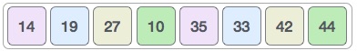
Then, we take interval of 2 and this gap generates two sub-lists
- `{14, 27, 35, 42}`, `{19, 10, 33, 44}`
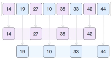
We compare and swap the values, if required, in the original array.
After this step, the array should look like this

> UPD: On the picture below there is a typo and result array is supposed to be `[14, 10, 27, 19, 35, 33, 42, 44]`.
Finally, we sort the rest of the array using interval of value 1.
Shell sort uses insertion sort to sort the array.
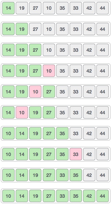
## Complexity
| Name | Best | Average | Worst | Memory | Stable | Comments |
| --------------------- | :-------------: | :-----------------: | :-----------------: | :-------: | :-------: | :-------- |
| **Shell sort** | n log(n) | depends on gap sequence | n (log(n))2 | 1 | No | |
## References
- [Tutorials Point](https://www.tutorialspoint.com/data_structures_algorithms/shell_sort_algorithm.htm)
- [Wikipedia](https://en.wikipedia.org/wiki/Shellsort)
- [YouTube by Rob Edwards](https://www.youtube.com/watch?v=ddeLSDsYVp8&index=79&list=PLLXdhg_r2hKA7DPDsunoDZ-Z769jWn4R8)
================================================
FILE: src/algorithms/sorting/shell-sort/README.pt-BR.md
================================================
# Shellsort
_Leia isso em outros idiomas:_
[_English_](README.md).
Shellsort, também conhecido como Shell sort ou método de Shell,
é uma classificação de comparação in-loco. Pode ser visto tanto como um
generalização da ordenação por troca (bubble sort) ou ordenação
por inserção (ordenação por inserção). O método começa classificando
pares de elementos distantes um do outro, então progressivamente
reduzindo a distância entre os elementos a serem comparados. Iniciando
com elementos distantes, pode mover alguns fora do lugar
elementos em posição mais rápido do que um simples vizinho mais próximo
intercâmbio

## Como o Shellsort funciona?
Para nosso exemplo e facilidade de compreensão, tomamos o intervalo
de `4`. Faça uma sub-lista virtual de todos os valores localizados no
intervalo de 4 posições. Aqui esses valores são
`{35, 14}`, `{33, 19}`, `{42, 27}` e `{10, 44}`

Comparamos valores em cada sublista e os trocamos (se necessário)
na matriz original. Após esta etapa, o novo array deve
parece com isso

Então, pegamos o intervalo de 2 e essa lacuna gera duas sub-listas
- `{14, 27, 35, 42}`, `{19, 10, 33, 44}`

Comparamos e trocamos os valores, se necessário, no array original.
Após esta etapa, a matriz deve ficar assim

> OBS: Na imagem abaixo há um erro de digitação e a matriz de resultados deve ser `[14, 10, 27, 19, 35, 33, 42, 44]`.
Finalmente, ordenamos o resto do array usando o intervalo de valor 1.
A classificação de shell usa a classificação por inserção para classificar a matriz.

## Complexidade
| Nome | Melhor | Média | Pior | Memória | Estável | Comentários |
| --------------------- | :-------------: | :-----------------: | :-----------------: | :-------: | :-------: | :-------- |
| **Shell sort** | n log(n) | depends on gap sequence | n (log(n))2 | 1 | Não | |
## Referências
- [Tutorials Point](https://www.tutorialspoint.com/data_structures_algorithms/shell_sort_algorithm.htm)
- [Wikipedia](https://en.wikipedia.org/wiki/Shellsort)
- [YouTube by Rob Edwards](https://www.youtube.com/watch?v=ddeLSDsYVp8&index=79&list=PLLXdhg_r2hKA7DPDsunoDZ-Z769jWn4R8)
================================================
FILE: src/algorithms/sorting/shell-sort/ShellSort.js
================================================
import Sort from '../Sort';
export default class ShellSort extends Sort {
sort(originalArray) {
// Prevent original array from mutations.
const array = [...originalArray];
// Define a gap distance.
let gap = Math.floor(array.length / 2);
// Until gap is bigger then zero do elements comparisons and swaps.
while (gap > 0) {
// Go and compare all distant element pairs.
for (let i = 0; i < (array.length - gap); i += 1) {
let currentIndex = i;
let gapShiftedIndex = i + gap;
while (currentIndex >= 0) {
// Call visiting callback.
this.callbacks.visitingCallback(array[currentIndex]);
// Compare and swap array elements if needed.
if (this.comparator.lessThan(array[gapShiftedIndex], array[currentIndex])) {
const tmp = array[currentIndex];
array[currentIndex] = array[gapShiftedIndex];
array[gapShiftedIndex] = tmp;
}
gapShiftedIndex = currentIndex;
currentIndex -= gap;
}
}
// Shrink the gap.
gap = Math.floor(gap / 2);
}
// Return sorted copy of an original array.
return array;
}
}
================================================
FILE: src/algorithms/sorting/shell-sort/__test__/ShellSort.test.js
================================================
import ShellSort from '../ShellSort';
import {
equalArr,
notSortedArr,
reverseArr,
sortedArr,
SortTester,
} from '../../SortTester';
// Complexity constants.
const SORTED_ARRAY_VISITING_COUNT = 320;
const NOT_SORTED_ARRAY_VISITING_COUNT = 320;
const REVERSE_SORTED_ARRAY_VISITING_COUNT = 320;
const EQUAL_ARRAY_VISITING_COUNT = 320;
describe('ShellSort', () => {
it('should sort array', () => {
SortTester.testSort(ShellSort);
});
it('should sort array with custom comparator', () => {
SortTester.testSortWithCustomComparator(ShellSort);
});
it('should sort negative numbers', () => {
SortTester.testNegativeNumbersSort(ShellSort);
});
it('should visit EQUAL array element specified number of times', () => {
SortTester.testAlgorithmTimeComplexity(
ShellSort,
equalArr,
EQUAL_ARRAY_VISITING_COUNT,
);
});
it('should visit SORTED array element specified number of times', () => {
SortTester.testAlgorithmTimeComplexity(
ShellSort,
sortedArr,
SORTED_ARRAY_VISITING_COUNT,
);
});
it('should visit NOT SORTED array element specified number of times', () => {
SortTester.testAlgorithmTimeComplexity(
ShellSort,
notSortedArr,
NOT_SORTED_ARRAY_VISITING_COUNT,
);
});
it('should visit REVERSE SORTED array element specified number of times', () => {
SortTester.testAlgorithmTimeComplexity(
ShellSort,
reverseArr,
REVERSE_SORTED_ARRAY_VISITING_COUNT,
);
});
});
================================================
FILE: src/algorithms/stack/valid-parentheses/README.md
================================================
# Valid Parentheses Problem
Given a string s containing just the characters '(', ')', '{', '}', '[' and ']', determine if the input string is valid.
An input string is valid if:
Open brackets must be closed by the same type of brackets.
Open brackets must be closed in the correct order.
Every close bracket has a corresponding open bracket of the same type.
Example 1:
`Input: s = "()"`
Output: true
Example 2:
`Input: s = "()[]{}"`
Output: true
Example 3:
`Input: s = "(]"`
Output: false
This is actually a very common interview question and a very good example of how to use a stack data structure to solve problems.
## Solution
The problem can be solved in two ways
### Bruteforce Approach
We can iterate through the string and then for each character in the string, we check for it's last closing character in the the string. Once we find the last closing character in the string, we remove both characters and then repeat the iteration, if we don't find a closing character for an opening character, then the string is invalid. The time complexity of this would be O(n^2) which is not so efficient.
### Using a Stack
We can use a hashtable to store all opening characters and the value would be the respective closing character. We can then iterate through the string and if we encounter an opening parantheses, we push it's closing character to the stack. If we ecounter a closing paraentheses, then we pop the stack and confirm that the popped element is equal to the current closing parentheses character. If it is not then the string is invalid. At the end of the iteration, we also need to check that the stack is empty. If it is not then the string is invalid. If it is, then the string is valid. This is a more efficient approach with a Time complexity and Space complexity of O(n).
## References
- [Leetcode](https://leetcode.com/problems/valid-parentheses/)
================================================
FILE: src/algorithms/stack/valid-parentheses/__test__/validParentheses.test.js
================================================
import isValid from '../validParentheses';
describe('validParentheses', () => {
it('should return false when string is empty', () => {
expect(isValid('')).toBe(false);
});
it('should return true when string contains valid parentheses in correct order', () => {
expect(isValid('()')).toBe(true);
expect(isValid('()[]{}')).toBe(true);
expect(isValid('((({[]})))')).toBe(true);
});
it('should return false when string contains invalid parentheses', () => {
expect(isValid('(]')).toBe(false);
expect(isValid('()[]{} }')).toBe(false);
expect(isValid('((({[(]})))')).toBe(false);
});
it('should return false when string contains valid parentheses in wrong order', () => {
expect(isValid('({)}')).toBe(false);
});
});
================================================
FILE: src/algorithms/stack/valid-parentheses/validParentheses.js
================================================
import Stack from '../../../data-structures/stack/Stack';
import HashTable from '../../../data-structures/hash-table/HashTable';
// Declare hashtable containg opening parentheses as key and it's closing parentheses as value.
const hashTable = new HashTable(3);
hashTable.set('{', '}');
hashTable.set('(', ')');
hashTable.set('[', ']');
/**
* Check if string has valid parentheses.
*
* @param {string} parenthesesString
* @return {boolean}
*/
export default function isValid(parenthesesString) {
// If string is empty return false
if (parenthesesString.length === 0) {
return false;
}
// Create stack
const stack = new Stack();
// Loop through each character of string
for (let i = 0; i < parenthesesString.length; i += 1) {
const currentCharacter = parenthesesString[i];
// If character is opening parentheses push it's closing parentheses to stack
if (hashTable.has(currentCharacter)) {
stack.push(hashTable.get(currentCharacter));
} else {
/* If character is a closing parentheses then,:
check If stack is empty, if it is return false.
if stack is not empty, pop from stack and compare it with current character.
If they are not same return false. */
if (stack.isEmpty() || stack.pop() !== currentCharacter) {
return false;
}
}
}
// If stack is empty return true else return false
return stack.isEmpty();
}
================================================
FILE: src/algorithms/statistics/weighted-random/README.md
================================================
# Weighted Random

## What is "Weighted Random"
Let's say you have a list of **items**. Item could be anything. For example, we may have a list of fruits and vegetables that you like to eat: `[ '🍌', '🍎', '🥕' ]`.
The list of **weights** represent the weight (or probability, or importance) of each item. Weights are numbers. For example, the weights like `[3, 7, 1]` would say that:
- you would like to eat `🍎 apples` more often (`7` out of `3 + 7 + 1 = 11` times),
- then you would like to eat `bananas 🍌` less often (only `3` out of `11` times),
- and the `carrots 🥕` you really don't like (want to eat it only `1` out of `11` times).
> If we speak in terms of probabilities than the weights list might be an array of floats that sum up to `1` (i.e. `[0.1, 0.5, 0.2, 0.2]`).
The **Weighted Random** in this case will be the function that will randomly return you the item from the list, and it will take each item's weight into account, so that items with the higher weight will be picked more often.
Example of the function interface:
```javascript
const items = [ '🍌', '🍎', '🥕' ];
const weights = [ 3, 7, 1 ];
function weightedRandom(items, weights) {
// implementation goes here ...
}
const nextSnackToEat = weightedRandom(items, weights); // Could be '🍎'
```
## Applications of Weighted Random
- In [Genetic Algorithm](https://en.wikipedia.org/wiki/Genetic_algorithm) the weighted random is used during the "Selection" phase, when we need to select the fittest/strongest individuums based on their fitness score for mating and for producing the next stronger generation. You may find an **example** in the [Self-Parking Car in 500 Lines of Code](https://trekhleb.dev/blog/2021/self-parking-car-evolution/) article.
- In [Recurrent Neural Networks (RNN)](https://en.wikipedia.org/wiki/Recurrent_neural_network) when trying to decide what letter to choose next (to form the sentence) based on the next letter probability. You may find an **example** in the [Recipe Generation using Recurrent Neural Network (RNN)](https://nbviewer.org/github/trekhleb/machine-learning-experiments/blob/master/experiments/recipe_generation_rnn/recipe_generation_rnn.ipynb) Jupyter notebook.
- In [Nginx Load Balancing](https://docs.nginx.com/nginx/admin-guide/load-balancer/http-load-balancer/) to send HTTP requests more often to the servers with the higher weights.
- And more...
## The Algorithm
The **straightforward approach** would be to:
1. Repeat each item in the list according to its weight.
2. Pick the random item from the list.
For example in our case with fruits and vegetables we could generate the following list of size `3 + 7 + 1 = 11`:
```javascript
const items = [ '🍌', '🍎', '🥕' ];
const weights = [ 3, 7, 1 ];
// Repeating the items based on weights.
const weightedItems = [
'🍌', '🍌', '🍌',
'🍎', '🍎', '🍎', '🍎', '🍎', '🍎', '🍎',
'🥕',
];
// And now just pick the random item from weightedItems array.
```
However, as you may see, this approach may require a lot of memory, in case if we have a lot of items to repeat in `weightedItems` list. Think of it as if you would need to repeat a string like `"some-random-string"` (`18` bytes) a ten million times. You will need to allocate around `180Mb` of additional memory space just for this array.
The **more efficient approach** would be to:
1. Prepare the list of cumulative weights for each item (i.e. the `cumulativeWeights` list which will have the same number of elements as the original `weights` list). In our case it will look like this: `cumulativeWeights = [3, 3 + 7, 3 + 7 + 1] = [3, 10, 11]`
2. Generate the random number `randomNumber` from `0` to the highest cumulative weight value. In our case the random number will be in a range of `[0..11]`. Let's say that we have `randomNumber = 8`.
3. Go through the `cumulativeWeights` list from left to right and pick the first element which is higher or equal to the `randomNumber`. The index of such element we will use to pick the item from the `items` array.
The idea behind this approach is that the higher weights will "occupy" more numeric space. Therefore, there is a higher chance that the random number will fall into the "higher weight numeric bucket".
```javascript
const weights = [3, 7, 1 ];
const cumulativeWeights = [3, 10, 11];
// In a pseudo-representation we may think about the cumulativeWeights array like this.
const pseudoCumulativeWeights = [
1, 2, 3, // <-- [3] numbers
4, 5, 6, 7, 8, 9, 10, // <-- [7] numbers
11, // <-- [1] number
];
```
Here is an example of how the `weightedRandom` function might be implemented:
```javascript
/**
* Picks the random item based on its weight.
* The items with higher weight will be picked more often (with a higher probability).
*
* For example:
* - items = ['banana', 'orange', 'apple']
* - weights = [0, 0.2, 0.8]
* - weightedRandom(items, weights) in 80% of cases will return 'apple', in 20% of cases will return
* 'orange' and it will never return 'banana' (because probability of picking the banana is 0%)
*
* @param {any[]} items
* @param {number[]} weights
* @returns {{item: any, index: number}}
*/
export default function weightedRandom(items, weights) {
if (items.length !== weights.length) {
throw new Error('Items and weights must be of the same size');
}
if (!items.length) {
throw new Error('Items must not be empty');
}
// Preparing the cumulative weights array.
// For example:
// - weights = [1, 4, 3]
// - cumulativeWeights = [1, 5, 8]
const cumulativeWeights = [];
for (let i = 0; i < weights.length; i += 1) {
cumulativeWeights[i] = weights[i] + (cumulativeWeights[i - 1] || 0);
}
// Getting the random number in a range of [0...sum(weights)]
// For example:
// - weights = [1, 4, 3]
// - maxCumulativeWeight = 8
// - range for the random number is [0...8]
const maxCumulativeWeight = cumulativeWeights[cumulativeWeights.length - 1];
const randomNumber = maxCumulativeWeight * Math.random();
// Picking the random item based on its weight.
// The items with higher weight will be picked more often.
for (let itemIndex = 0; itemIndex < items.length; itemIndex += 1) {
if (cumulativeWeights[itemIndex] >= randomNumber) {
return {
item: items[itemIndex],
index: itemIndex,
};
}
}
}
```
## Implementation
- Check the [weightedRandom.js](weightedRandom.js) file for the implementation of the `weightedRandom()` function.
- Check the [weightedRandom.test.js](__test__/weightedRandom.test.js) file for the tests-cases.
================================================
FILE: src/algorithms/statistics/weighted-random/__test__/weightedRandom.test.js
================================================
import weightedRandom from '../weightedRandom';
describe('weightedRandom', () => {
it('should throw an error when the number of weights does not match the number of items', () => {
const getWeightedRandomWithInvalidInputs = () => {
weightedRandom(['a', 'b', 'c'], [10, 0]);
};
expect(getWeightedRandomWithInvalidInputs).toThrow('Items and weights must be of the same size');
});
it('should throw an error when the number of weights or items are empty', () => {
const getWeightedRandomWithInvalidInputs = () => {
weightedRandom([], []);
};
expect(getWeightedRandomWithInvalidInputs).toThrow('Items must not be empty');
});
it('should correctly do random selection based on wights in straightforward cases', () => {
expect(weightedRandom(['a', 'b', 'c'], [1, 0, 0])).toEqual({ index: 0, item: 'a' });
expect(weightedRandom(['a', 'b', 'c'], [0, 1, 0])).toEqual({ index: 1, item: 'b' });
expect(weightedRandom(['a', 'b', 'c'], [0, 0, 1])).toEqual({ index: 2, item: 'c' });
expect(weightedRandom(['a', 'b', 'c'], [0, 1, 1])).not.toEqual({ index: 0, item: 'a' });
expect(weightedRandom(['a', 'b', 'c'], [1, 0, 1])).not.toEqual({ index: 1, item: 'b' });
expect(weightedRandom(['a', 'b', 'c'], [1, 1, 0])).not.toEqual({ index: 2, item: 'c' });
});
it('should correctly do random selection based on wights', () => {
// Number of times we're going to select the random items based on their weights.
const ATTEMPTS_NUM = 1000;
// The +/- delta in the number of times each item has been actually selected.
// I.e. if we want the item 'a' to be selected 300 times out of 1000 cases (30%)
// then 267 times is acceptable since it is bigger that 250 (which is 300 - 50)
// ans smaller than 350 (which is 300 + 50)
const THRESHOLD = 50;
const items = ['a', 'b', 'c']; // The actual items values don't matter.
const weights = [0.1, 0.3, 0.6];
const counter = [];
for (let i = 0; i < ATTEMPTS_NUM; i += 1) {
const randomItem = weightedRandom(items, weights);
if (!counter[randomItem.index]) {
counter[randomItem.index] = 1;
} else {
counter[randomItem.index] += 1;
}
}
for (let itemIndex = 0; itemIndex < items.length; itemIndex += 1) {
/*
i.e. item with the index of 0 must be selected 100 times (ideally)
or with the threshold of [100 - 50, 100 + 50] times.
i.e. item with the index of 1 must be selected 300 times (ideally)
or with the threshold of [300 - 50, 300 + 50] times.
i.e. item with the index of 2 must be selected 600 times (ideally)
or with the threshold of [600 - 50, 600 + 50] times.
*/
expect(counter[itemIndex]).toBeGreaterThan(ATTEMPTS_NUM * weights[itemIndex] - THRESHOLD);
expect(counter[itemIndex]).toBeLessThan(ATTEMPTS_NUM * weights[itemIndex] + THRESHOLD);
}
});
});
================================================
FILE: src/algorithms/statistics/weighted-random/weightedRandom.js
================================================
/**
* Picks the random item based on its weight.
* The items with higher weight will be picked more often (with a higher probability).
*
* For example:
* - items = ['banana', 'orange', 'apple']
* - weights = [0, 0.2, 0.8]
* - weightedRandom(items, weights) in 80% of cases will return 'apple', in 20% of cases will return
* 'orange' and it will never return 'banana' (because probability of picking the banana is 0%)
*
* @param {any[]} items
* @param {number[]} weights
* @returns {{item: any, index: number}}
*/
/* eslint-disable consistent-return */
export default function weightedRandom(items, weights) {
if (items.length !== weights.length) {
throw new Error('Items and weights must be of the same size');
}
if (!items.length) {
throw new Error('Items must not be empty');
}
// Preparing the cumulative weights array.
// For example:
// - weights = [1, 4, 3]
// - cumulativeWeights = [1, 5, 8]
const cumulativeWeights = [];
for (let i = 0; i < weights.length; i += 1) {
cumulativeWeights[i] = weights[i] + (cumulativeWeights[i - 1] || 0);
}
// Getting the random number in a range of [0...sum(weights)]
// For example:
// - weights = [1, 4, 3]
// - maxCumulativeWeight = 8
// - range for the random number is [0...8]
const maxCumulativeWeight = cumulativeWeights[cumulativeWeights.length - 1];
const randomNumber = maxCumulativeWeight * Math.random();
// Picking the random item based on its weight.
// The items with higher weight will be picked more often.
for (let itemIndex = 0; itemIndex < items.length; itemIndex += 1) {
if (cumulativeWeights[itemIndex] >= randomNumber) {
return {
item: items[itemIndex],
index: itemIndex,
};
}
}
}
================================================
FILE: src/algorithms/string/hamming-distance/README.md
================================================
# Hamming Distance
the Hamming distance between two strings of equal length is the
number of positions at which the corresponding symbols are
different. In other words, it measures the minimum number of
substitutions required to change one string into the other, or
the minimum number of errors that could have transformed one
string into the other. In a more general context, the Hamming
distance is one of several string metrics for measuring the
edit distance between two sequences.
## Examples
The Hamming distance between:
- "ka**rol**in" and "ka**thr**in" is **3**.
- "k**a**r**ol**in" and "k**e**r**st**in" is **3**.
- 10**1**1**1**01 and 10**0**1**0**01 is **2**.
- 2**17**3**8**96 and 2**23**3**7**96 is **3**.
## References
[Wikipedia](https://en.wikipedia.org/wiki/Hamming_distance)
================================================
FILE: src/algorithms/string/hamming-distance/__test__/hammingDistance.test.js
================================================
import hammingDistance from '../hammingDistance';
describe('hammingDistance', () => {
it('should throw an error when trying to compare the strings of different lengths', () => {
const compareStringsOfDifferentLength = () => {
hammingDistance('a', 'aa');
};
expect(compareStringsOfDifferentLength).toThrow();
});
it('should calculate difference between two strings', () => {
expect(hammingDistance('a', 'a')).toBe(0);
expect(hammingDistance('a', 'b')).toBe(1);
expect(hammingDistance('abc', 'add')).toBe(2);
expect(hammingDistance('karolin', 'kathrin')).toBe(3);
expect(hammingDistance('karolin', 'kerstin')).toBe(3);
expect(hammingDistance('1011101', '1001001')).toBe(2);
expect(hammingDistance('2173896', '2233796')).toBe(3);
});
});
================================================
FILE: src/algorithms/string/hamming-distance/hammingDistance.js
================================================
/**
* @param {string} a
* @param {string} b
* @return {number}
*/
export default function hammingDistance(a, b) {
if (a.length !== b.length) {
throw new Error('Strings must be of the same length');
}
let distance = 0;
for (let i = 0; i < a.length; i += 1) {
if (a[i] !== b[i]) {
distance += 1;
}
}
return distance;
}
================================================
FILE: src/algorithms/string/knuth-morris-pratt/README.md
================================================
# Knuth–Morris–Pratt Algorithm
The Knuth–Morris–Pratt string searching algorithm (or
KMP algorithm) searches for occurrences of a "word" `W`
within a main "text string" `T` by employing the
observation that when a mismatch occurs, the word itself
embodies sufficient information to determine where the
next match could begin, thus bypassing re-examination
of previously matched characters.
## Complexity
- **Time:** `O(|W| + |T|)` (much faster comparing to trivial `O(|W| * |T|)`)
- **Space:** `O(|W|)`
## References
- [Wikipedia](https://en.wikipedia.org/wiki/Knuth%E2%80%93Morris%E2%80%93Pratt_algorithm)
- [YouTube](https://www.youtube.com/watch?v=GTJr8OvyEVQ&list=PLLXdhg_r2hKA7DPDsunoDZ-Z769jWn4R8)
================================================
FILE: src/algorithms/string/knuth-morris-pratt/__test__/knuthMorrisPratt.test.js
================================================
import knuthMorrisPratt from '../knuthMorrisPratt';
describe('knuthMorrisPratt', () => {
it('should find word position in given text', () => {
expect(knuthMorrisPratt('', '')).toBe(0);
expect(knuthMorrisPratt('a', '')).toBe(0);
expect(knuthMorrisPratt('a', 'a')).toBe(0);
expect(knuthMorrisPratt('abcbcglx', 'abca')).toBe(-1);
expect(knuthMorrisPratt('abcbcglx', 'bcgl')).toBe(3);
expect(knuthMorrisPratt('abcxabcdabxabcdabcdabcy', 'abcdabcy')).toBe(15);
expect(knuthMorrisPratt('abcxabcdabxabcdabcdabcy', 'abcdabca')).toBe(-1);
expect(knuthMorrisPratt('abcxabcdabxaabcdabcabcdabcdabcy', 'abcdabca')).toBe(12);
expect(knuthMorrisPratt('abcxabcdabxaabaabaaaabcdabcdabcy', 'aabaabaaa')).toBe(11);
});
});
================================================
FILE: src/algorithms/string/knuth-morris-pratt/knuthMorrisPratt.js
================================================
/**
* @see https://www.youtube.com/watch?v=GTJr8OvyEVQ
* @param {string} word
* @return {number[]}
*/
function buildPatternTable(word) {
const patternTable = [0];
let prefixIndex = 0;
let suffixIndex = 1;
while (suffixIndex < word.length) {
if (word[prefixIndex] === word[suffixIndex]) {
patternTable[suffixIndex] = prefixIndex + 1;
suffixIndex += 1;
prefixIndex += 1;
} else if (prefixIndex === 0) {
patternTable[suffixIndex] = 0;
suffixIndex += 1;
} else {
prefixIndex = patternTable[prefixIndex - 1];
}
}
return patternTable;
}
/**
* @param {string} text
* @param {string} word
* @return {number}
*/
export default function knuthMorrisPratt(text, word) {
if (word.length === 0) {
return 0;
}
let textIndex = 0;
let wordIndex = 0;
const patternTable = buildPatternTable(word);
while (textIndex < text.length) {
if (text[textIndex] === word[wordIndex]) {
// We've found a match.
if (wordIndex === word.length - 1) {
return (textIndex - word.length) + 1;
}
wordIndex += 1;
textIndex += 1;
} else if (wordIndex > 0) {
wordIndex = patternTable[wordIndex - 1];
} else {
// wordIndex = 0;
textIndex += 1;
}
}
return -1;
}
================================================
FILE: src/algorithms/string/levenshtein-distance/README.md
================================================
# Levenshtein Distance
The Levenshtein distance is a string metric for measuring the
difference between two sequences. Informally, the Levenshtein
distance between two words is the minimum number of
single-character edits (insertions, deletions or substitutions)
required to change one word into the other.
## Definition
Mathematically, the Levenshtein distance between two strings
`a` and `b` (of length `|a|` and `|b|` respectively) is given by

where

where

is the indicator function equal to `0` when

and equal to 1 otherwise, and

is the distance between the first `i` characters of `a` and the first
`j` characters of `b`.
Note that the first element in the minimum corresponds to
deletion (from `a` to `b`), the second to insertion and
the third to match or mismatch, depending on whether the
respective symbols are the same.
## Example
For example, the Levenshtein distance between `kitten` and
`sitting` is `3`, since the following three edits change one
into the other, and there is no way to do it with fewer than
three edits:
1. **k**itten → **s**itten (substitution of "s" for "k")
2. sitt**e**n → sitt**i**n (substitution of "i" for "e")
3. sittin → sittin**g** (insertion of "g" at the end).
## Applications
This has a wide range of applications, for instance, spell checkers, correction
systems for optical character recognition, fuzzy string searching, and software
to assist natural language translation based on translation memory.
## Dynamic Programming Approach Explanation
Let’s take a simple example of finding minimum edit distance between
strings `ME` and `MY`. Intuitively you already know that minimum edit distance
here is `1` operation, which is replacing `E` with `Y`. But
let’s try to formalize it in a form of the algorithm in order to be able to
do more complex examples like transforming `Saturday` into `Sunday`.
To apply the mathematical formula mentioned above to `ME → MY` transformation
we need to know minimum edit distances of `ME → M`, `M → MY` and `M → M` transformations
in prior. Then we will need to pick the minimum one and add _one_ operation to
transform last letters `E → Y`. So minimum edit distance of `ME → MY` transformation
is being calculated based on three previously possible transformations.
To explain this further let’s draw the following matrix:
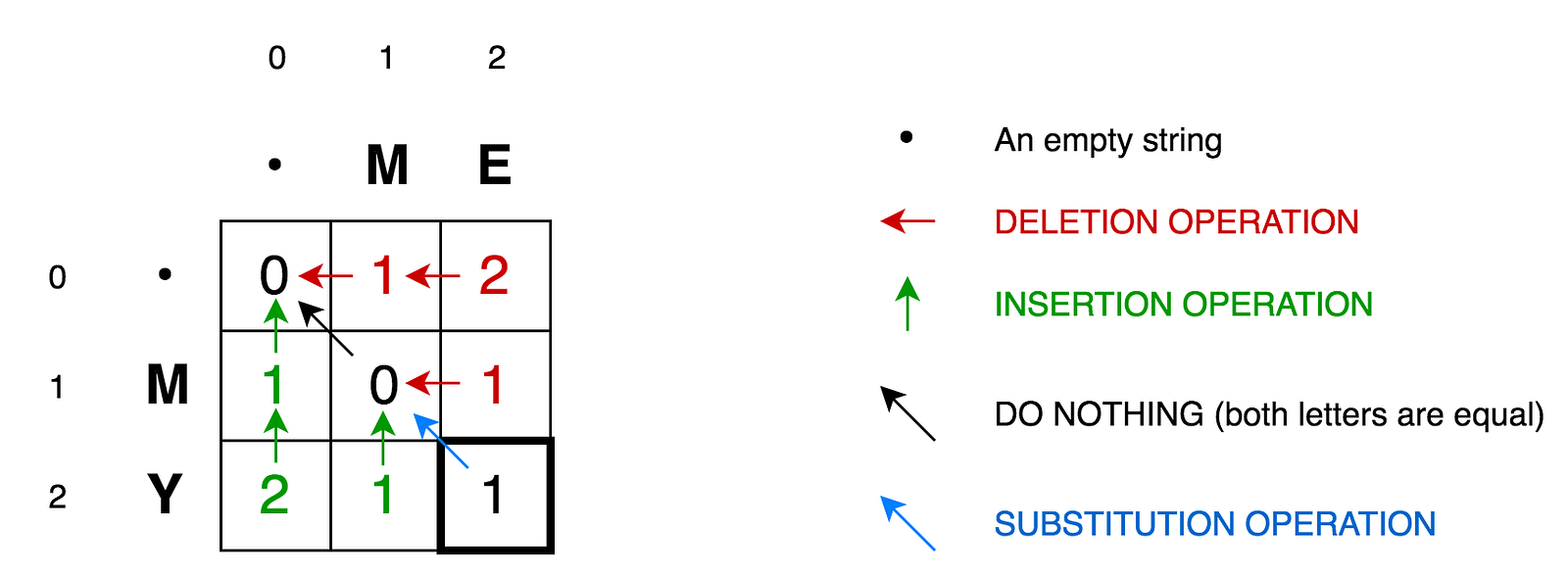
- Cell `(0:1)` contains red number 1. It means that we need 1 operation to
transform `M` to an empty string. And it is by deleting `M`. This is why this number is red.
- Cell `(0:2)` contains red number 2. It means that we need 2 operations
to transform `ME` to an empty string. And it is by deleting `E` and `M`.
- Cell `(1:0)` contains green number 1. It means that we need 1 operation
to transform an empty string to `M`. And it is by inserting `M`. This is why this number is green.
- Cell `(2:0)` contains green number 2. It means that we need 2 operations
to transform an empty string to `MY`. And it is by inserting `Y` and `M`.
- Cell `(1:1)` contains number 0. It means that it costs nothing
to transform `M` into `M`.
- Cell `(1:2)` contains red number 1. It means that we need 1 operation
to transform `ME` to `M`. And it is by deleting `E`.
- And so on...
This looks easy for such small matrix as ours (it is only `3x3`). But here you
may find basic concepts that may be applied to calculate all those numbers for
bigger matrices (let’s say a `9x7` matrix for `Saturday → Sunday` transformation).
According to the formula you only need three adjacent cells `(i-1:j)`, `(i-1:j-1)`, and `(i:j-1)` to
calculate the number for current cell `(i:j)`. All we need to do is to find the
minimum of those three cells and then add `1` in case if we have different
letters in `i`'s row and `j`'s column.
You may clearly see the recursive nature of the problem.
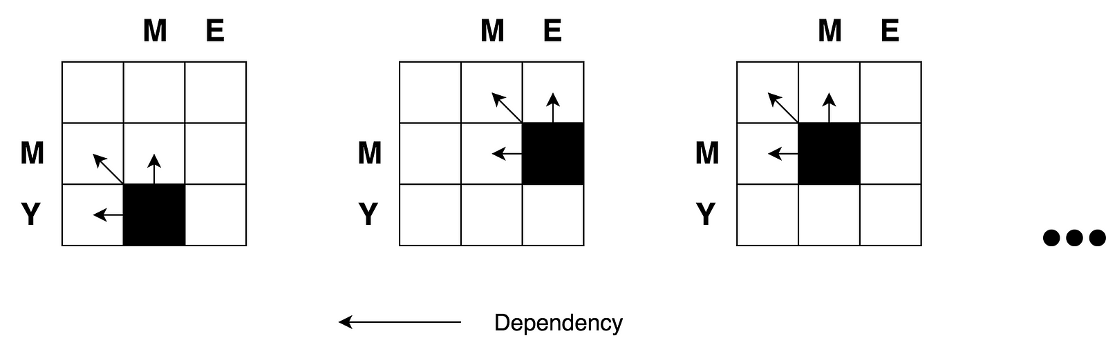
Let's draw a decision graph for this problem.
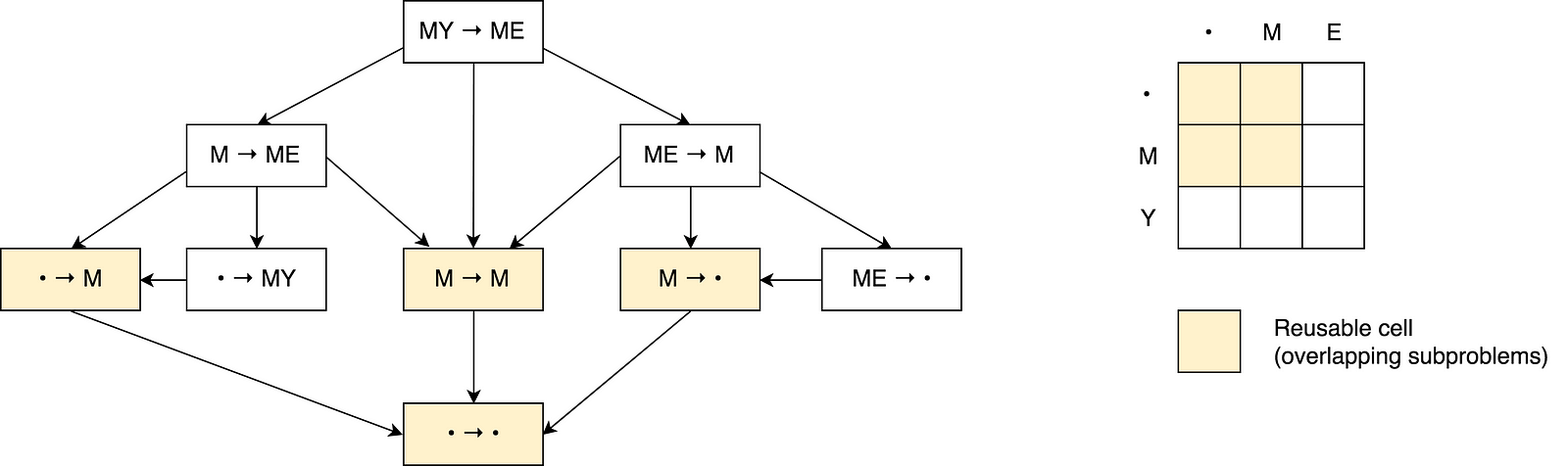
You may see a number of overlapping sub-problems on the picture that are marked
with red. Also there is no way to reduce the number of operations and make it
less than a minimum of those three adjacent cells from the formula.
Also you may notice that each cell number in the matrix is being calculated
based on previous ones. Thus the tabulation technique (filling the cache in
bottom-up direction) is being applied here.
Applying this principle further we may solve more complicated cases like
with `Saturday → Sunday` transformation.
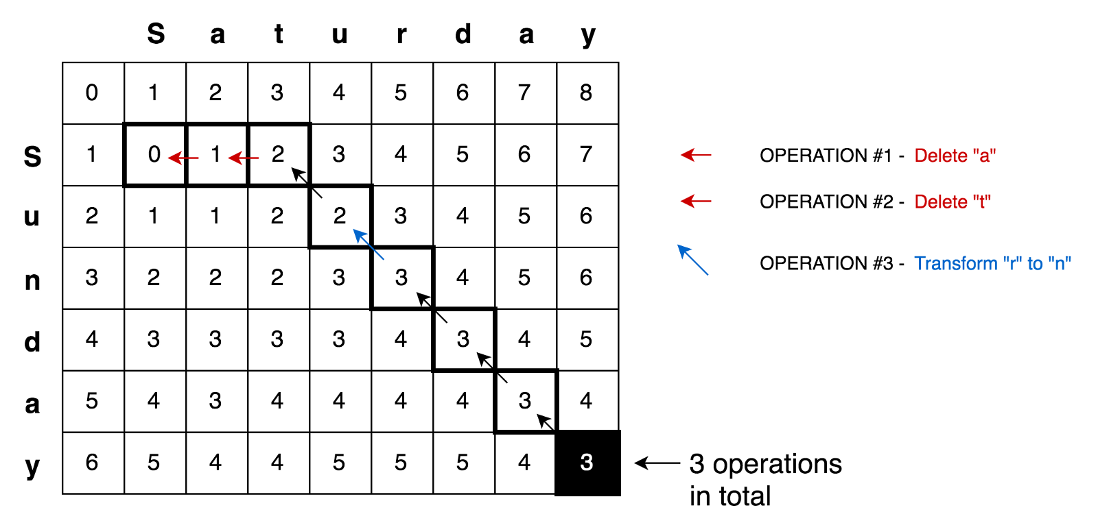
## References
- [Wikipedia](https://en.wikipedia.org/wiki/Levenshtein_distance)
- [YouTube](https://www.youtube.com/watch?v=We3YDTzNXEk&list=PLLXdhg_r2hKA7DPDsunoDZ-Z769jWn4R8)
- [ITNext](https://itnext.io/dynamic-programming-vs-divide-and-conquer-2fea680becbe)
================================================
FILE: src/algorithms/string/levenshtein-distance/__test__/levenshteinDistance.test.js
================================================
import levenshteinDistance from '../levenshteinDistance';
describe('levenshteinDistance', () => {
it('should calculate edit distance between two strings', () => {
expect(levenshteinDistance('', '')).toBe(0);
expect(levenshteinDistance('a', '')).toBe(1);
expect(levenshteinDistance('', 'a')).toBe(1);
expect(levenshteinDistance('abc', '')).toBe(3);
expect(levenshteinDistance('', 'abc')).toBe(3);
// Should just add I to the beginning.
expect(levenshteinDistance('islander', 'slander')).toBe(1);
// Needs to substitute M by K, T by M and add an A to the end
expect(levenshteinDistance('mart', 'karma')).toBe(3);
// Substitute K by S, E by I and insert G at the end.
expect(levenshteinDistance('kitten', 'sitting')).toBe(3);
// Should add 4 letters FOOT at the beginning.
expect(levenshteinDistance('ball', 'football')).toBe(4);
// Should delete 4 letters FOOT at the beginning.
expect(levenshteinDistance('football', 'foot')).toBe(4);
// Needs to substitute the first 5 chars: INTEN by EXECU
expect(levenshteinDistance('intention', 'execution')).toBe(5);
});
});
================================================
FILE: src/algorithms/string/levenshtein-distance/levenshteinDistance.js
================================================
/**
* @param {string} a
* @param {string} b
* @return {number}
*/
export default function levenshteinDistance(a, b) {
// Create empty edit distance matrix for all possible modifications of
// substrings of a to substrings of b.
const distanceMatrix = Array(b.length + 1).fill(null).map(() => Array(a.length + 1).fill(null));
// Fill the first row of the matrix.
// If this is first row then we're transforming empty string to a.
// In this case the number of transformations equals to size of a substring.
for (let i = 0; i <= a.length; i += 1) {
distanceMatrix[0][i] = i;
}
// Fill the first column of the matrix.
// If this is first column then we're transforming empty string to b.
// In this case the number of transformations equals to size of b substring.
for (let j = 0; j <= b.length; j += 1) {
distanceMatrix[j][0] = j;
}
for (let j = 1; j <= b.length; j += 1) {
for (let i = 1; i <= a.length; i += 1) {
const indicator = a[i - 1] === b[j - 1] ? 0 : 1;
distanceMatrix[j][i] = Math.min(
distanceMatrix[j][i - 1] + 1, // deletion
distanceMatrix[j - 1][i] + 1, // insertion
distanceMatrix[j - 1][i - 1] + indicator, // substitution
);
}
}
return distanceMatrix[b.length][a.length];
}
================================================
FILE: src/algorithms/string/longest-common-substring/README.md
================================================
# Longest Common Substring Problem
The longest common substring problem is to find the longest string
(or strings) that is a substring (or are substrings) of two or more
strings.
## Example
The longest common substring of the strings `ABABC`, `BABCA` and
`ABCBA` is string `ABC` of length 3. Other common substrings are
`A`, `AB`, `B`, `BA`, `BC` and `C`.
```
ABABC
|||
BABCA
|||
ABCBA
```
## References
- [Wikipedia](https://en.wikipedia.org/wiki/Longest_common_substring_problem)
- [YouTube](https://www.youtube.com/watch?v=BysNXJHzCEs&list=PLLXdhg_r2hKA7DPDsunoDZ-Z769jWn4R8)
================================================
FILE: src/algorithms/string/longest-common-substring/__test__/longestCommonSubstring.test.js
================================================
import longestCommonSubstring from '../longestCommonSubstring';
describe('longestCommonSubstring', () => {
it('should find longest common substring between two strings', () => {
expect(longestCommonSubstring('', '')).toBe('');
expect(longestCommonSubstring('ABC', '')).toBe('');
expect(longestCommonSubstring('', 'ABC')).toBe('');
expect(longestCommonSubstring('ABABC', 'BABCA')).toBe('BABC');
expect(longestCommonSubstring('BABCA', 'ABCBA')).toBe('ABC');
expect(longestCommonSubstring('sea', 'eat')).toBe('ea');
expect(longestCommonSubstring('algorithms', 'rithm')).toBe('rithm');
expect(longestCommonSubstring(
'Algorithms and data structures implemented in JavaScript',
'Here you may find Algorithms and data structures that are implemented in JavaScript',
)).toBe('Algorithms and data structures ');
});
it('should handle unicode correctly', () => {
expect(longestCommonSubstring('𐌵𐌵**ABC', '𐌵𐌵--ABC')).toBe('ABC');
expect(longestCommonSubstring('𐌵𐌵**A', '𐌵𐌵--A')).toBe('𐌵𐌵');
expect(longestCommonSubstring('A买B时', '买B时GD')).toBe('买B时');
expect(longestCommonSubstring('After test买时 case', 'another_test买时')).toBe('test买时');
});
});
================================================
FILE: src/algorithms/string/longest-common-substring/longestCommonSubstring.js
================================================
/**
* Longest Common Substring (LCS) (Dynamic Programming Approach).
*
* @param {string} string1
* @param {string} string2
* @return {string}
*/
export default function longestCommonSubstring(string1, string2) {
// Convert strings to arrays to treat unicode symbols length correctly.
// For example:
// '𐌵'.length === 2
// [...'𐌵'].length === 1
const s1 = [...string1];
const s2 = [...string2];
// Init the matrix of all substring lengths to use Dynamic Programming approach.
const substringMatrix = Array(s2.length + 1).fill(null).map(() => {
return Array(s1.length + 1).fill(null);
});
// Fill the first row and first column with zeros to provide initial values.
for (let columnIndex = 0; columnIndex <= s1.length; columnIndex += 1) {
substringMatrix[0][columnIndex] = 0;
}
for (let rowIndex = 0; rowIndex <= s2.length; rowIndex += 1) {
substringMatrix[rowIndex][0] = 0;
}
// Build the matrix of all substring lengths to use Dynamic Programming approach.
let longestSubstringLength = 0;
let longestSubstringColumn = 0;
let longestSubstringRow = 0;
for (let rowIndex = 1; rowIndex <= s2.length; rowIndex += 1) {
for (let columnIndex = 1; columnIndex <= s1.length; columnIndex += 1) {
if (s1[columnIndex - 1] === s2[rowIndex - 1]) {
substringMatrix[rowIndex][columnIndex] = substringMatrix[rowIndex - 1][columnIndex - 1] + 1;
} else {
substringMatrix[rowIndex][columnIndex] = 0;
}
// Try to find the biggest length of all common substring lengths
// and to memorize its last character position (indices)
if (substringMatrix[rowIndex][columnIndex] > longestSubstringLength) {
longestSubstringLength = substringMatrix[rowIndex][columnIndex];
longestSubstringColumn = columnIndex;
longestSubstringRow = rowIndex;
}
}
}
if (longestSubstringLength === 0) {
// Longest common substring has not been found.
return '';
}
// Detect the longest substring from the matrix.
let longestSubstring = '';
while (substringMatrix[longestSubstringRow][longestSubstringColumn] > 0) {
longestSubstring = s1[longestSubstringColumn - 1] + longestSubstring;
longestSubstringRow -= 1;
longestSubstringColumn -= 1;
}
return longestSubstring;
}
================================================
FILE: src/algorithms/string/palindrome/README.md
================================================
# Palindrome Check
A [Palindrome](https://en.wikipedia.org/wiki/Palindrome) is a string that reads the same forwards and backwards.
This means that the second half of the string is the reverse of the
first half.
## Examples
The following are palindromes (thus would return `TRUE`):
```
- "a"
- "pop" -> p + o + p
- "deed" -> de + ed
- "kayak" -> ka + y + ak
- "racecar" -> rac + e + car
```
The following are NOT palindromes (thus would return `FALSE`):
```
- "rad"
- "dodo"
- "polo"
```
## References
- [GeeksForGeeks - Check if a number is Palindrome](https://www.geeksforgeeks.org/check-if-a-number-is-palindrome/)
================================================
FILE: src/algorithms/string/palindrome/__test__/isPalindrome.test.js
================================================
import isPalindrome from '../isPalindrome';
describe('palindromeCheck', () => {
it('should return whether or not the string is a palindrome', () => {
expect(isPalindrome('a')).toBe(true);
expect(isPalindrome('pop')).toBe(true);
expect(isPalindrome('deed')).toBe(true);
expect(isPalindrome('kayak')).toBe(true);
expect(isPalindrome('racecar')).toBe(true);
expect(isPalindrome('rad')).toBe(false);
expect(isPalindrome('dodo')).toBe(false);
expect(isPalindrome('polo')).toBe(false);
});
});
================================================
FILE: src/algorithms/string/palindrome/isPalindrome.js
================================================
/**
* @param {string} string
* @return {boolean}
*/
export default function isPalindrome(string) {
let left = 0;
let right = string.length - 1;
while (left < right) {
if (string[left] !== string[right]) {
return false;
}
left += 1;
right -= 1;
}
return true;
}
================================================
FILE: src/algorithms/string/rabin-karp/README.md
================================================
# Rabin Karp Algorithm
In computer science, the Rabin–Karp algorithm or Karp–Rabin algorithm
is a string searching algorithm created by Richard M. Karp and
Michael O. Rabin (1987) that uses hashing to find any one of a set
of pattern strings in a text.
## Algorithm
The Rabin–Karp algorithm seeks to speed up the testing of equality of
the pattern to the substrings in the text by using a hash function. A
hash function is a function which converts every string into a numeric
value, called its hash value; for example, we might
have `hash('hello') = 5`. The algorithm exploits the fact
that if two strings are equal, their hash values are also equal. Thus,
string matching is reduced (almost) to computing the hash value of the
search pattern and then looking for substrings of the input string with
that hash value.
However, there are two problems with this approach. First, because there
are so many different strings and so few hash values, some differing
strings will have the same hash value. If the hash values match, the
pattern and the substring may not match; consequently, the potential
match of search pattern and the substring must be confirmed by comparing
them; that comparison can take a long time for long substrings.
Luckily, a good hash function on reasonable strings usually does not
have many collisions, so the expected search time will be acceptable.
## Hash Function Used
The key to the Rabin–Karp algorithm's performance is the efficient computation
of hash values of the successive substrings of the text.
The **Rabin fingerprint** is a popular and effective rolling hash function.
The **polynomial hash function** described in this example is not a Rabin
fingerprint, but it works equally well. It treats every substring as a
number in some base, the base being usually a large prime.
## Complexity
For text of length `n` and `p` patterns of combined length `m`, its average
and best case running time is `O(n + m)` in space `O(p)`, but its
worst-case time is `O(n * m)`.
## Application
A practical application of the algorithm is detecting plagiarism.
Given source material, the algorithm can rapidly search through a paper
for instances of sentences from the source material, ignoring details
such as case and punctuation. Because of the abundance of the sought
strings, single-string searching algorithms are impractical.
## References
- [Wikipedia](https://en.wikipedia.org/wiki/Rabin%E2%80%93Karp_algorithm)
- [YouTube](https://www.youtube.com/watch?v=H4VrKHVG5qI&list=PLLXdhg_r2hKA7DPDsunoDZ-Z769jWn4R8)
================================================
FILE: src/algorithms/string/rabin-karp/__test__/rabinKarp.test.js
================================================
import rabinKarp from '../rabinKarp';
describe('rabinKarp', () => {
it('should find substring in a string', () => {
expect(rabinKarp('', '')).toBe(0);
expect(rabinKarp('a', '')).toBe(0);
expect(rabinKarp('a', 'a')).toBe(0);
expect(rabinKarp('ab', 'b')).toBe(1);
expect(rabinKarp('abcbcglx', 'abca')).toBe(-1);
expect(rabinKarp('abcbcglx', 'bcgl')).toBe(3);
expect(rabinKarp('abcxabcdabxabcdabcdabcy', 'abcdabcy')).toBe(15);
expect(rabinKarp('abcxabcdabxabcdabcdabcy', 'abcdabca')).toBe(-1);
expect(rabinKarp('abcxabcdabxaabcdabcabcdabcdabcy', 'abcdabca')).toBe(12);
expect(rabinKarp('abcxabcdabxaabaabaaaabcdabcdabcy', 'aabaabaaa')).toBe(11);
expect(rabinKarp('^ !/\'#\'pp', ' !/\'#\'pp')).toBe(1);
});
it('should work with bigger texts', () => {
const text = 'Lorem Ipsum is simply dummy text of the printing and '
+ 'typesetting industry. Lorem Ipsum has been the industry\'s standard '
+ 'dummy text ever since the 1500s, when an unknown printer took a '
+ 'galley of type and scrambled it to make a type specimen book. It '
+ 'has survived not only five centuries, but also the leap into '
+ 'electronic typesetting, remaining essentially unchanged. It was '
+ 'popularised in the 1960s with the release of Letraset sheets '
+ 'containing Lorem Ipsum passages, and more recently with desktop'
+ 'publishing software like Aldus PageMaker including versions of Lorem '
+ 'Ipsum.';
expect(rabinKarp(text, 'Lorem')).toBe(0);
expect(rabinKarp(text, 'versions')).toBe(549);
expect(rabinKarp(text, 'versions of Lorem Ipsum.')).toBe(549);
expect(rabinKarp(text, 'versions of Lorem Ipsum:')).toBe(-1);
expect(rabinKarp(text, 'Lorem Ipsum passages, and more recently with')).toBe(446);
});
it('should work with UTF symbols', () => {
expect(rabinKarp('a\u{ffff}', '\u{ffff}')).toBe(1);
expect(rabinKarp('\u0000耀\u0000', '耀\u0000')).toBe(1);
// @TODO: Provide Unicode support.
// expect(rabinKarp('a\u{20000}', '\u{20000}')).toBe(1);
});
});
================================================
FILE: src/algorithms/string/rabin-karp/rabinKarp.js
================================================
import PolynomialHash from '../../cryptography/polynomial-hash/PolynomialHash';
/**
* @param {string} text - Text that may contain the searchable word.
* @param {string} word - Word that is being searched in text.
* @return {number} - Position of the word in text.
*/
export default function rabinKarp(text, word) {
const hasher = new PolynomialHash();
// Calculate word hash that we will use for comparison with other substring hashes.
const wordHash = hasher.hash(word);
let prevFrame = null;
let currentFrameHash = null;
// Go through all substring of the text that may match.
for (let charIndex = 0; charIndex <= (text.length - word.length); charIndex += 1) {
const currentFrame = text.substring(charIndex, charIndex + word.length);
// Calculate the hash of current substring.
if (currentFrameHash === null) {
currentFrameHash = hasher.hash(currentFrame);
} else {
currentFrameHash = hasher.roll(currentFrameHash, prevFrame, currentFrame);
}
prevFrame = currentFrame;
// Compare the hash of current substring and seeking string.
// In case if hashes match let's make sure that substrings are equal.
// In case of hash collision the strings may not be equal.
if (
wordHash === currentFrameHash
&& text.substr(charIndex, word.length) === word
) {
return charIndex;
}
}
return -1;
}
================================================
FILE: src/algorithms/string/regular-expression-matching/README.md
================================================
# Regular Expression Matching
Given an input string `s` and a pattern `p`, implement regular
expression matching with support for `.` and `*`.
- `.` Matches any single character.
- `*` Matches zero or more of the preceding element.
The matching should cover the **entire** input string (not partial).
**Note**
- `s` could be empty and contains only lowercase letters `a-z`.
- `p` could be empty and contains only lowercase letters `a-z`, and characters like `.` or `*`.
## Examples
**Example #1**
Input:
```
s = 'aa'
p = 'a'
```
Output: `false`
Explanation: `a` does not match the entire string `aa`.
**Example #2**
Input:
```
s = 'aa'
p = 'a*'
```
Output: `true`
Explanation: `*` means zero or more of the preceding element, `a`.
Therefore, by repeating `a` once, it becomes `aa`.
**Example #3**
Input:
```
s = 'ab'
p = '.*'
```
Output: `true`
Explanation: `.*` means "zero or more (`*`) of any character (`.`)".
**Example #4**
Input:
```
s = 'aab'
p = 'c*a*b'
```
Output: `true`
Explanation: `c` can be repeated 0 times, `a` can be repeated
1 time. Therefore it matches `aab`.
## References
- [YouTube](https://www.youtube.com/watch?v=l3hda49XcDE&list=PLLXdhg_r2hKA7DPDsunoDZ-Z769jWn4R8&index=71&t=0s)
- [LeetCode](https://leetcode.com/problems/regular-expression-matching/description/)
================================================
FILE: src/algorithms/string/regular-expression-matching/__test__/regularExpressionMatching.test.js
================================================
import regularExpressionMatching from '../regularExpressionMatching';
describe('regularExpressionMatching', () => {
it('should match regular expressions in a string', () => {
expect(regularExpressionMatching('', '')).toBe(true);
expect(regularExpressionMatching('a', 'a')).toBe(true);
expect(regularExpressionMatching('aa', 'aa')).toBe(true);
expect(regularExpressionMatching('aab', 'aab')).toBe(true);
expect(regularExpressionMatching('aab', 'aa.')).toBe(true);
expect(regularExpressionMatching('aab', '.a.')).toBe(true);
expect(regularExpressionMatching('aab', '...')).toBe(true);
expect(regularExpressionMatching('a', 'a*')).toBe(true);
expect(regularExpressionMatching('aaa', 'a*')).toBe(true);
expect(regularExpressionMatching('aaab', 'a*b')).toBe(true);
expect(regularExpressionMatching('aaabb', 'a*b*')).toBe(true);
expect(regularExpressionMatching('aaabb', 'a*b*c*')).toBe(true);
expect(regularExpressionMatching('', 'a*')).toBe(true);
expect(regularExpressionMatching('xaabyc', 'xa*b.c')).toBe(true);
expect(regularExpressionMatching('aab', 'c*a*b*')).toBe(true);
expect(regularExpressionMatching('mississippi', 'mis*is*.p*.')).toBe(true);
expect(regularExpressionMatching('ab', '.*')).toBe(true);
expect(regularExpressionMatching('', 'a')).toBe(false);
expect(regularExpressionMatching('a', '')).toBe(false);
expect(regularExpressionMatching('aab', 'aa')).toBe(false);
expect(regularExpressionMatching('aab', 'baa')).toBe(false);
expect(regularExpressionMatching('aabc', '...')).toBe(false);
expect(regularExpressionMatching('aaabbdd', 'a*b*c*')).toBe(false);
expect(regularExpressionMatching('mississippi', 'mis*is*p*.')).toBe(false);
expect(regularExpressionMatching('ab', 'a*')).toBe(false);
expect(regularExpressionMatching('abba', 'a*b*.c')).toBe(false);
expect(regularExpressionMatching('abba', '.*c')).toBe(false);
});
});
================================================
FILE: src/algorithms/string/regular-expression-matching/regularExpressionMatching.js
================================================
const ZERO_OR_MORE_CHARS = '*';
const ANY_CHAR = '.';
/**
* Dynamic programming approach.
*
* @param {string} string
* @param {string} pattern
* @return {boolean}
*/
export default function regularExpressionMatching(string, pattern) {
/*
* Let's initiate dynamic programming matrix for this string and pattern.
* We will have pattern characters on top (as columns) and string characters
* will be placed to the left of the table (as rows).
*
* Example:
*
* a * b . b
* - - - - - -
* a - - - - - -
* a - - - - - -
* b - - - - - -
* y - - - - - -
* b - - - - - -
*/
const matchMatrix = Array(string.length + 1).fill(null).map(() => {
return Array(pattern.length + 1).fill(null);
});
// Let's fill the top-left cell with true. This would mean that empty
// string '' matches to empty pattern ''.
matchMatrix[0][0] = true;
// Let's fill the first row of the matrix with false. That would mean that
// empty string can't match any non-empty pattern.
//
// Example:
// string: ''
// pattern: 'a.z'
//
// The one exception here is patterns like a*b* that matches the empty string.
for (let columnIndex = 1; columnIndex <= pattern.length; columnIndex += 1) {
const patternIndex = columnIndex - 1;
if (pattern[patternIndex] === ZERO_OR_MORE_CHARS) {
matchMatrix[0][columnIndex] = matchMatrix[0][columnIndex - 2];
} else {
matchMatrix[0][columnIndex] = false;
}
}
// Let's fill the first column with false. That would mean that empty pattern
// can't match any non-empty string.
//
// Example:
// string: 'ab'
// pattern: ''
for (let rowIndex = 1; rowIndex <= string.length; rowIndex += 1) {
matchMatrix[rowIndex][0] = false;
}
// Not let's go through every letter of the pattern and every letter of
// the string and compare them one by one.
for (let rowIndex = 1; rowIndex <= string.length; rowIndex += 1) {
for (let columnIndex = 1; columnIndex <= pattern.length; columnIndex += 1) {
// Take into account that fact that matrix contain one extra column and row.
const stringIndex = rowIndex - 1;
const patternIndex = columnIndex - 1;
if (pattern[patternIndex] === ZERO_OR_MORE_CHARS) {
/*
* In case if current pattern character is special '*' character we have
* two options:
*
* 1. Since * char allows it previous char to not be presented in a string we
* need to check if string matches the pattern without '*' char and without the
* char that goes before '*'. That would mean to go two positions left on the
* same row.
*
* 2. Since * char allows it previous char to be presented in a string many times we
* need to check if char before * is the same as current string char. If they are the
* same that would mean that current string matches the current pattern in case if
* the string WITHOUT current char matches the same pattern. This would mean to go
* one position up in the same row.
*/
if (matchMatrix[rowIndex][columnIndex - 2] === true) {
matchMatrix[rowIndex][columnIndex] = true;
} else if (
(
pattern[patternIndex - 1] === string[stringIndex]
|| pattern[patternIndex - 1] === ANY_CHAR
)
&& matchMatrix[rowIndex - 1][columnIndex] === true
) {
matchMatrix[rowIndex][columnIndex] = true;
} else {
matchMatrix[rowIndex][columnIndex] = false;
}
} else if (
pattern[patternIndex] === string[stringIndex]
|| pattern[patternIndex] === ANY_CHAR
) {
/*
* In case if current pattern char is the same as current string char
* or it may be any character (in case if pattern contains '.' char)
* we need to check if there was a match for the pattern and for the
* string by WITHOUT current char. This would mean that we may copy
* left-top diagonal value.
*
* Example:
*
* a b
* a 1 -
* b - 1
*/
matchMatrix[rowIndex][columnIndex] = matchMatrix[rowIndex - 1][columnIndex - 1];
} else {
/*
* In case if pattern char and string char are different we may
* treat this case as "no-match".
*
* Example:
*
* a b
* a - -
* c - 0
*/
matchMatrix[rowIndex][columnIndex] = false;
}
}
}
return matchMatrix[string.length][pattern.length];
}
================================================
FILE: src/algorithms/string/z-algorithm/README.md
================================================
# Z Algorithm
The Z-algorithm finds occurrences of a "word" `W`
within a main "text string" `T` in linear time `O(|W| + |T|)`.
Given a string `S` of length `n`, the algorithm produces
an array, `Z` where `Z[i]` represents the longest substring
starting from `S[i]` which is also a prefix of `S`. Finding
`Z` for the string obtained by concatenating the word, `W`
with a nonce character, say `$` followed by the text, `T`,
helps with pattern matching, for if there is some index `i`
such that `Z[i]` equals the pattern length, then the pattern
must be present at that point.
While the `Z` array can be computed with two nested loops in `O(|W| * |T|)` time, the
following strategy shows how to obtain it in linear time, based
on the idea that as we iterate over the letters in the string
(index `i` from `1` to `n - 1`), we maintain an interval `[L, R]`
which is the interval with maximum `R` such that `1 ≤ L ≤ i ≤ R`
and `S[L...R]` is a prefix that is also a substring (if no such
interval exists, just let `L = R = - 1`). For `i = 1`, we can
simply compute `L` and `R` by comparing `S[0...]` to `S[1...]`.
**Example of Z array**
```
Index 0 1 2 3 4 5 6 7 8 9 10 11
Text a a b c a a b x a a a z
Z values X 1 0 0 3 1 0 0 2 2 1 0
```
Other examples
```
str = a a a a a a
Z[] = x 5 4 3 2 1
```
```
str = a a b a a c d
Z[] = x 1 0 2 1 0 0
```
```
str = a b a b a b a b
Z[] = x 0 6 0 4 0 2 0
```
**Example of Z box**

## Complexity
- **Time:** `O(|W| + |T|)`
- **Space:** `O(|W|)`
## References
- [GeeksForGeeks](https://www.geeksforgeeks.org/z-algorithm-linear-time-pattern-searching-algorithm/)
- [YouTube](https://www.youtube.com/watch?v=CpZh4eF8QBw&t=0s&list=PLLXdhg_r2hKA7DPDsunoDZ-Z769jWn4R8&index=70)
- [Z Algorithm by Ivan Yurchenko](https://ivanyu.me/blog/2013/10/15/z-algorithm/)
================================================
FILE: src/algorithms/string/z-algorithm/__test__/zAlgorithm.test.js
================================================
import zAlgorithm from '../zAlgorithm';
describe('zAlgorithm', () => {
it('should find word positions in given text', () => {
expect(zAlgorithm('abcbcglx', 'abca')).toEqual([]);
expect(zAlgorithm('abca', 'abca')).toEqual([0]);
expect(zAlgorithm('abca', 'abcadfd')).toEqual([]);
expect(zAlgorithm('abcbcglabcx', 'abc')).toEqual([0, 7]);
expect(zAlgorithm('abcbcglx', 'bcgl')).toEqual([3]);
expect(zAlgorithm('abcbcglx', 'cglx')).toEqual([4]);
expect(zAlgorithm('abcxabcdabxabcdabcdabcy', 'abcdabcy')).toEqual([15]);
expect(zAlgorithm('abcxabcdabxabcdabcdabcy', 'abcdabca')).toEqual([]);
expect(zAlgorithm('abcxabcdabxaabcdabcabcdabcdabcy', 'abcdabca')).toEqual([12]);
expect(zAlgorithm('abcxabcdabxaabaabaaaabcdabcdabcy', 'aabaabaaa')).toEqual([11]);
});
});
================================================
FILE: src/algorithms/string/z-algorithm/zAlgorithm.js
================================================
// The string separator that is being used for "word" and "text" concatenation.
const SEPARATOR = '$';
/**
* @param {string} zString
* @return {number[]}
*/
function buildZArray(zString) {
// Initiate zArray and fill it with zeros.
const zArray = new Array(zString.length).fill(null).map(() => 0);
// Z box boundaries.
let zBoxLeftIndex = 0;
let zBoxRightIndex = 0;
// Position of current zBox character that is also a position of
// the same character in prefix.
// For example:
// Z string: ab$xxabxx
// Indices: 012345678
// Prefix: ab.......
// Z box: .....ab..
// Z box shift for 'a' would be 0 (0-position in prefix and 0-position in Z box)
// Z box shift for 'b' would be 1 (1-position in prefix and 1-position in Z box)
let zBoxShift = 0;
// Go through all characters of the zString.
for (let charIndex = 1; charIndex < zString.length; charIndex += 1) {
if (charIndex > zBoxRightIndex) {
// We're OUTSIDE of Z box. In other words this is a case when we're
// starting from Z box of size 1.
// In this case let's make current character to be a Z box of length 1.
zBoxLeftIndex = charIndex;
zBoxRightIndex = charIndex;
// Now let's go and check current and the following characters to see if
// they are the same as a prefix. By doing this we will also expand our
// Z box. For example if starting from current position we will find 3
// more characters that are equal to the ones in the prefix we will expand
// right Z box boundary by 3.
while (
zBoxRightIndex < zString.length
&& zString[zBoxRightIndex - zBoxLeftIndex] === zString[zBoxRightIndex]
) {
// Expanding Z box right boundary.
zBoxRightIndex += 1;
}
// Now we may calculate how many characters starting from current position
// are are the same as the prefix. We may calculate it by difference between
// right and left Z box boundaries.
zArray[charIndex] = zBoxRightIndex - zBoxLeftIndex;
// Move right Z box boundary left by one position just because we've used
// [zBoxRightIndex - zBoxLeftIndex] index calculation above.
zBoxRightIndex -= 1;
} else {
// We're INSIDE of Z box.
// Calculate corresponding Z box shift. Because we want to copy the values
// from zArray that have been calculated before.
zBoxShift = charIndex - zBoxLeftIndex;
// Check if the value that has been already calculated before
// leaves us inside of Z box or it goes beyond the checkbox
// right boundary.
if (zArray[zBoxShift] < (zBoxRightIndex - charIndex) + 1) {
// If calculated value don't force us to go outside Z box
// then we're safe and we may simply use previously calculated value.
zArray[charIndex] = zArray[zBoxShift];
} else {
// In case if previously calculated values forces us to go outside of Z box
// we can't safely copy previously calculated zArray value. It is because
// we are sure that there is no further prefix matches outside of Z box.
// Thus such values must be re-calculated and reduced to certain point.
// To do so we need to shift left boundary of Z box to current position.
zBoxLeftIndex = charIndex;
// And start comparing characters one by one as we normally do for the case
// when we are outside of checkbox.
while (
zBoxRightIndex < zString.length
&& zString[zBoxRightIndex - zBoxLeftIndex] === zString[zBoxRightIndex]
) {
zBoxRightIndex += 1;
}
zArray[charIndex] = zBoxRightIndex - zBoxLeftIndex;
zBoxRightIndex -= 1;
}
}
}
// Return generated zArray.
return zArray;
}
/**
* @param {string} text
* @param {string} word
* @return {number[]}
*/
export default function zAlgorithm(text, word) {
// The list of word's positions in text. Word may be found in the same text
// in several different positions. Thus it is an array.
const wordPositions = [];
// Concatenate word and string. Word will be a prefix to a string.
const zString = `${word}${SEPARATOR}${text}`;
// Generate Z-array for concatenated string.
const zArray = buildZArray(zString);
// Based on Z-array properties each cell will tell us the length of the match between
// the string prefix and current sub-text. Thus we're may find all positions in zArray
// with the number that equals to the length of the word (zString prefix) and based on
// that positions we'll be able to calculate word positions in text.
for (let charIndex = 1; charIndex < zArray.length; charIndex += 1) {
if (zArray[charIndex] === word.length) {
// Since we did concatenation to form zString we need to subtract prefix
// and separator lengths.
const wordPosition = charIndex - word.length - SEPARATOR.length;
wordPositions.push(wordPosition);
}
}
// Return the list of word positions.
return wordPositions;
}
================================================
FILE: src/algorithms/tree/breadth-first-search/README.md
================================================
# Breadth-First Search (BFS)
Breadth-first search (BFS) is an algorithm for traversing
or searching tree or graph data structures. It starts at
the tree root (or some arbitrary node of a graph, sometimes
referred to as a 'search key') and explores the neighbor
nodes first, before moving to the next level neighbors.

## Pseudocode
```text
BFS(root)
Pre: root is the node of the BST
Post: the nodes in the BST have been visited in breadth first order
q ← queue
while root = ø
yield root.value
if root.left = ø
q.enqueue(root.left)
end if
if root.right = ø
q.enqueue(root.right)
end if
if !q.isEmpty()
root ← q.dequeue()
else
root ← ø
end if
end while
end BFS
```
## References
- [Wikipedia](https://en.wikipedia.org/wiki/Breadth-first_search)
- [Tree Traversals (Inorder, Preorder and Postorder)](https://www.geeksforgeeks.org/tree-traversals-inorder-preorder-and-postorder/)
- [BFS vs DFS](https://www.geeksforgeeks.org/bfs-vs-dfs-binary-tree/)
================================================
FILE: src/algorithms/tree/breadth-first-search/__test__/breadthFirstSearch.test.js
================================================
import BinaryTreeNode from '../../../../data-structures/tree/BinaryTreeNode';
import breadthFirstSearch from '../breadthFirstSearch';
describe('breadthFirstSearch', () => {
it('should perform BFS operation on tree', () => {
const nodeA = new BinaryTreeNode('A');
const nodeB = new BinaryTreeNode('B');
const nodeC = new BinaryTreeNode('C');
const nodeD = new BinaryTreeNode('D');
const nodeE = new BinaryTreeNode('E');
const nodeF = new BinaryTreeNode('F');
const nodeG = new BinaryTreeNode('G');
nodeA.setLeft(nodeB).setRight(nodeC);
nodeB.setLeft(nodeD).setRight(nodeE);
nodeC.setLeft(nodeF).setRight(nodeG);
// In-order traversing.
expect(nodeA.toString()).toBe('D,B,E,A,F,C,G');
const enterNodeCallback = jest.fn();
const leaveNodeCallback = jest.fn();
// Traverse tree without callbacks first to check default ones.
breadthFirstSearch(nodeA);
// Traverse tree with callbacks.
breadthFirstSearch(nodeA, {
enterNode: enterNodeCallback,
leaveNode: leaveNodeCallback,
});
expect(enterNodeCallback).toHaveBeenCalledTimes(7);
expect(leaveNodeCallback).toHaveBeenCalledTimes(7);
// Check node entering.
expect(enterNodeCallback.mock.calls[0][0].value).toEqual('A');
expect(enterNodeCallback.mock.calls[1][0].value).toEqual('B');
expect(enterNodeCallback.mock.calls[2][0].value).toEqual('C');
expect(enterNodeCallback.mock.calls[3][0].value).toEqual('D');
expect(enterNodeCallback.mock.calls[4][0].value).toEqual('E');
expect(enterNodeCallback.mock.calls[5][0].value).toEqual('F');
expect(enterNodeCallback.mock.calls[6][0].value).toEqual('G');
// Check node leaving.
expect(leaveNodeCallback.mock.calls[0][0].value).toEqual('A');
expect(leaveNodeCallback.mock.calls[1][0].value).toEqual('B');
expect(leaveNodeCallback.mock.calls[2][0].value).toEqual('C');
expect(leaveNodeCallback.mock.calls[3][0].value).toEqual('D');
expect(leaveNodeCallback.mock.calls[4][0].value).toEqual('E');
expect(leaveNodeCallback.mock.calls[5][0].value).toEqual('F');
expect(leaveNodeCallback.mock.calls[6][0].value).toEqual('G');
});
it('allow users to redefine node visiting logic', () => {
const nodeA = new BinaryTreeNode('A');
const nodeB = new BinaryTreeNode('B');
const nodeC = new BinaryTreeNode('C');
const nodeD = new BinaryTreeNode('D');
const nodeE = new BinaryTreeNode('E');
const nodeF = new BinaryTreeNode('F');
const nodeG = new BinaryTreeNode('G');
nodeA.setLeft(nodeB).setRight(nodeC);
nodeB.setLeft(nodeD).setRight(nodeE);
nodeC.setLeft(nodeF).setRight(nodeG);
// In-order traversing.
expect(nodeA.toString()).toBe('D,B,E,A,F,C,G');
const enterNodeCallback = jest.fn();
const leaveNodeCallback = jest.fn();
// Traverse tree without callbacks first to check default ones.
breadthFirstSearch(nodeA);
// Traverse tree with callbacks.
breadthFirstSearch(nodeA, {
allowTraversal: (node, child) => {
// Forbid traversing left half of the tree.
return child.value !== 'B';
},
enterNode: enterNodeCallback,
leaveNode: leaveNodeCallback,
});
expect(enterNodeCallback).toHaveBeenCalledTimes(4);
expect(leaveNodeCallback).toHaveBeenCalledTimes(4);
// Check node entering.
expect(enterNodeCallback.mock.calls[0][0].value).toEqual('A');
expect(enterNodeCallback.mock.calls[1][0].value).toEqual('C');
expect(enterNodeCallback.mock.calls[2][0].value).toEqual('F');
expect(enterNodeCallback.mock.calls[3][0].value).toEqual('G');
// Check node leaving.
expect(leaveNodeCallback.mock.calls[0][0].value).toEqual('A');
expect(leaveNodeCallback.mock.calls[1][0].value).toEqual('C');
expect(leaveNodeCallback.mock.calls[2][0].value).toEqual('F');
expect(leaveNodeCallback.mock.calls[3][0].value).toEqual('G');
});
});
================================================
FILE: src/algorithms/tree/breadth-first-search/breadthFirstSearch.js
================================================
import Queue from '../../../data-structures/queue/Queue';
/**
* @typedef {Object} Callbacks
* @property {function(node: BinaryTreeNode, child: BinaryTreeNode): boolean} allowTraversal -
* Determines whether BFS should traverse from the node to its child.
* @property {function(node: BinaryTreeNode)} enterNode - Called when BFS enters the node.
* @property {function(node: BinaryTreeNode)} leaveNode - Called when BFS leaves the node.
*/
/**
* @param {Callbacks} [callbacks]
* @returns {Callbacks}
*/
function initCallbacks(callbacks = {}) {
const initiatedCallback = callbacks;
const stubCallback = () => {};
const defaultAllowTraversal = () => true;
initiatedCallback.allowTraversal = callbacks.allowTraversal || defaultAllowTraversal;
initiatedCallback.enterNode = callbacks.enterNode || stubCallback;
initiatedCallback.leaveNode = callbacks.leaveNode || stubCallback;
return initiatedCallback;
}
/**
* @param {BinaryTreeNode} rootNode
* @param {Callbacks} [originalCallbacks]
*/
export default function breadthFirstSearch(rootNode, originalCallbacks) {
const callbacks = initCallbacks(originalCallbacks);
const nodeQueue = new Queue();
// Do initial queue setup.
nodeQueue.enqueue(rootNode);
while (!nodeQueue.isEmpty()) {
const currentNode = nodeQueue.dequeue();
callbacks.enterNode(currentNode);
// Add all children to the queue for future traversals.
// Traverse left branch.
if (currentNode.left && callbacks.allowTraversal(currentNode, currentNode.left)) {
nodeQueue.enqueue(currentNode.left);
}
// Traverse right branch.
if (currentNode.right && callbacks.allowTraversal(currentNode, currentNode.right)) {
nodeQueue.enqueue(currentNode.right);
}
callbacks.leaveNode(currentNode);
}
}
================================================
FILE: src/algorithms/tree/depth-first-search/README.md
================================================
# Depth-First Search (DFS)
Depth-first search (DFS) is an algorithm for traversing or
searching tree or graph data structures. One starts at
the root (selecting some arbitrary node as the root in
the case of a graph) and explores as far as possible
along each branch before backtracking.

## References
- [Wikipedia](https://en.wikipedia.org/wiki/Depth-first_search)
- [Tree Traversals (Inorder, Preorder and Postorder)](https://www.geeksforgeeks.org/tree-traversals-inorder-preorder-and-postorder/)
- [BFS vs DFS](https://www.geeksforgeeks.org/bfs-vs-dfs-binary-tree/)
================================================
FILE: src/algorithms/tree/depth-first-search/__test__/depthFirstSearch.test.js
================================================
import BinaryTreeNode from '../../../../data-structures/tree/BinaryTreeNode';
import depthFirstSearch from '../depthFirstSearch';
describe('depthFirstSearch', () => {
it('should perform DFS operation on tree', () => {
const nodeA = new BinaryTreeNode('A');
const nodeB = new BinaryTreeNode('B');
const nodeC = new BinaryTreeNode('C');
const nodeD = new BinaryTreeNode('D');
const nodeE = new BinaryTreeNode('E');
const nodeF = new BinaryTreeNode('F');
const nodeG = new BinaryTreeNode('G');
nodeA.setLeft(nodeB).setRight(nodeC);
nodeB.setLeft(nodeD).setRight(nodeE);
nodeC.setLeft(nodeF).setRight(nodeG);
// In-order traversing.
expect(nodeA.toString()).toBe('D,B,E,A,F,C,G');
const enterNodeCallback = jest.fn();
const leaveNodeCallback = jest.fn();
// Traverse tree without callbacks first to check default ones.
depthFirstSearch(nodeA);
// Traverse tree with callbacks.
depthFirstSearch(nodeA, {
enterNode: enterNodeCallback,
leaveNode: leaveNodeCallback,
});
expect(enterNodeCallback).toHaveBeenCalledTimes(7);
expect(leaveNodeCallback).toHaveBeenCalledTimes(7);
// Check node entering.
expect(enterNodeCallback.mock.calls[0][0].value).toEqual('A');
expect(enterNodeCallback.mock.calls[1][0].value).toEqual('B');
expect(enterNodeCallback.mock.calls[2][0].value).toEqual('D');
expect(enterNodeCallback.mock.calls[3][0].value).toEqual('E');
expect(enterNodeCallback.mock.calls[4][0].value).toEqual('C');
expect(enterNodeCallback.mock.calls[5][0].value).toEqual('F');
expect(enterNodeCallback.mock.calls[6][0].value).toEqual('G');
// Check node leaving.
expect(leaveNodeCallback.mock.calls[0][0].value).toEqual('D');
expect(leaveNodeCallback.mock.calls[1][0].value).toEqual('E');
expect(leaveNodeCallback.mock.calls[2][0].value).toEqual('B');
expect(leaveNodeCallback.mock.calls[3][0].value).toEqual('F');
expect(leaveNodeCallback.mock.calls[4][0].value).toEqual('G');
expect(leaveNodeCallback.mock.calls[5][0].value).toEqual('C');
expect(leaveNodeCallback.mock.calls[6][0].value).toEqual('A');
});
it('allow users to redefine node visiting logic', () => {
const nodeA = new BinaryTreeNode('A');
const nodeB = new BinaryTreeNode('B');
const nodeC = new BinaryTreeNode('C');
const nodeD = new BinaryTreeNode('D');
const nodeE = new BinaryTreeNode('E');
const nodeF = new BinaryTreeNode('F');
const nodeG = new BinaryTreeNode('G');
nodeA.setLeft(nodeB).setRight(nodeC);
nodeB.setLeft(nodeD).setRight(nodeE);
nodeC.setLeft(nodeF).setRight(nodeG);
// In-order traversing.
expect(nodeA.toString()).toBe('D,B,E,A,F,C,G');
const enterNodeCallback = jest.fn();
const leaveNodeCallback = jest.fn();
// Traverse tree without callbacks first to check default ones.
depthFirstSearch(nodeA);
// Traverse tree with callbacks.
depthFirstSearch(nodeA, {
allowTraversal: (node, child) => {
// Forbid traversing left part of the tree.
return child.value !== 'B';
},
enterNode: enterNodeCallback,
leaveNode: leaveNodeCallback,
});
expect(enterNodeCallback).toHaveBeenCalledTimes(4);
expect(leaveNodeCallback).toHaveBeenCalledTimes(4);
// Check node entering.
expect(enterNodeCallback.mock.calls[0][0].value).toEqual('A');
expect(enterNodeCallback.mock.calls[1][0].value).toEqual('C');
expect(enterNodeCallback.mock.calls[2][0].value).toEqual('F');
expect(enterNodeCallback.mock.calls[3][0].value).toEqual('G');
// Check node leaving.
expect(leaveNodeCallback.mock.calls[0][0].value).toEqual('F');
expect(leaveNodeCallback.mock.calls[1][0].value).toEqual('G');
expect(leaveNodeCallback.mock.calls[2][0].value).toEqual('C');
expect(leaveNodeCallback.mock.calls[3][0].value).toEqual('A');
});
});
================================================
FILE: src/algorithms/tree/depth-first-search/depthFirstSearch.js
================================================
/**
* @typedef {Object} TraversalCallbacks
*
* @property {function(node: BinaryTreeNode, child: BinaryTreeNode): boolean} allowTraversal
* - Determines whether DFS should traverse from the node to its child.
*
* @property {function(node: BinaryTreeNode)} enterNode - Called when DFS enters the node.
*
* @property {function(node: BinaryTreeNode)} leaveNode - Called when DFS leaves the node.
*/
/**
* Extend missing traversal callbacks with default callbacks.
*
* @param {TraversalCallbacks} [callbacks] - The object that contains traversal callbacks.
* @returns {TraversalCallbacks} - Traversal callbacks extended with defaults callbacks.
*/
function initCallbacks(callbacks = {}) {
// Init empty callbacks object.
const initiatedCallbacks = {};
// Empty callback that we will use in case if user didn't provide real callback function.
const stubCallback = () => {};
// By default we will allow traversal of every node
// in case if user didn't provide a callback for that.
const defaultAllowTraversalCallback = () => true;
// Copy original callbacks to our initiatedCallbacks object or use default callbacks instead.
initiatedCallbacks.allowTraversal = callbacks.allowTraversal || defaultAllowTraversalCallback;
initiatedCallbacks.enterNode = callbacks.enterNode || stubCallback;
initiatedCallbacks.leaveNode = callbacks.leaveNode || stubCallback;
// Returned processed list of callbacks.
return initiatedCallbacks;
}
/**
* Recursive depth-first-search traversal for binary.
*
* @param {BinaryTreeNode} node - binary tree node that we will start traversal from.
* @param {TraversalCallbacks} callbacks - the object that contains traversal callbacks.
*/
export function depthFirstSearchRecursive(node, callbacks) {
// Call the "enterNode" callback to notify that the node is going to be entered.
callbacks.enterNode(node);
// Traverse left branch only if case if traversal of the left node is allowed.
if (node.left && callbacks.allowTraversal(node, node.left)) {
depthFirstSearchRecursive(node.left, callbacks);
}
// Traverse right branch only if case if traversal of the right node is allowed.
if (node.right && callbacks.allowTraversal(node, node.right)) {
depthFirstSearchRecursive(node.right, callbacks);
}
// Call the "leaveNode" callback to notify that traversal
// of the current node and its children is finished.
callbacks.leaveNode(node);
}
/**
* Perform depth-first-search traversal of the rootNode.
* For every traversal step call "allowTraversal", "enterNode" and "leaveNode" callbacks.
* See TraversalCallbacks type definition for more details about the shape of callbacks object.
*
* @param {BinaryTreeNode} rootNode - The node from which we start traversing.
* @param {TraversalCallbacks} [callbacks] - Traversal callbacks.
*/
export default function depthFirstSearch(rootNode, callbacks) {
// In case if user didn't provide some callback we need to replace them with default ones.
const processedCallbacks = initCallbacks(callbacks);
// Now, when we have all necessary callbacks we may proceed to recursive traversal.
depthFirstSearchRecursive(rootNode, processedCallbacks);
}
================================================
FILE: src/algorithms/uncategorized/best-time-to-buy-sell-stocks/README.md
================================================
# Best Time to Buy and Sell Stock
## Task Description
Say you have an array prices for which the `i`-th element is the price of a given stock on day `i`.
Find the maximum profit. You may complete as many transactions as you like (i.e., buy one and sell one share of the stock multiple times).
> Note: You may not engage in multiple transactions at the same time (i.e., you must sell the stock before you buy again).
**Example #1**
```
Input: [7, 1, 5, 3, 6, 4]
Output: 7
```
_Explanation:_ Buy on day `2` (`price = 1`) and sell on day `3` (`price = 5`), `profit = 5-1 = 4`. Then buy on day `4` (`price = 3`) and sell on day `5` (`price = 6`), `profit = 6-3 = 3`.
**Example #2**
```
Input: [1, 2, 3, 4, 5]
Output: 4
```
_Explanation:_ Buy on day `1` (`price = 1`) and sell on day `5` (`price = 5`), `profit = 5-1 = 4`. Note that you cannot buy on day 1, buy on day 2 and sell them later, as you are engaging multiple transactions at the same time. You must sell before buying again.
**Example #3**
```
Input: [7, 6, 4, 3, 1]
Output: 0
```
_Explanation:_ In this case, no transaction is done, i.e. max `profit = 0`.
## Possible Solutions
### Divide and conquer approach `O(2^n)`
We may try **all** combinations of buying and selling and find out the most profitable one by applying _divide and conquer approach_.
Let's say we have an array of prices `[7, 6, 4, 3, 1]` and we're on the _1st_ day of trading (at the very beginning of the array). At this point we may say that the overall maximum profit would be the _maximum_ of two following values:
1. _Option 1: Keep the money_ → profit would equal to the profit from buying/selling the rest of the stocks → `keepProfit = profit([6, 4, 3, 1])`.
2. _Option 2: Buy/sell at current price_ → profit in this case would equal to the profit from buying/selling the rest of the stocks plus (or minus, depending on whether we're selling or buying) the current stock price → `buySellProfit = -7 + profit([6, 4, 3, 1])`.
The overall profit would be equal to → `overallProfit = Max(keepProfit, buySellProfit)`.
As you can see the `profit([6, 4, 3, 1])` task is being solved in the same recursive manner.
> See the full code example in [dqBestTimeToBuySellStocks.js](dqBestTimeToBuySellStocks.js)
#### Time Complexity
As you may see, every recursive call will produce _2_ more recursive branches. The depth of the recursion will be `n` (size of prices array) and thus, the time complexity will equal to `O(2^n)`.
As you may see, this is very inefficient. For example for just `20` prices the number of recursive calls will be somewhere close to `2M`!
#### Additional Space Complexity
If we avoid cloning the prices array between recursive function calls and will use the array pointer then additional space complexity will be proportional to the depth of the recursion: `O(n)`
## Peak Valley Approach `O(n)`
If we plot the prices array (i.e. `[7, 1, 5, 3, 6, 4]`) we may notice that the points of interest are the consecutive valleys and peaks

_Image source: [LeetCode](https://leetcode.com/problems/best-time-to-buy-and-sell-stock-ii/solution/)_
So, if we will track the growing price and will sell the stocks immediately _before_ the price goes down we'll get the maximum profit (remember, we bought the stock in the valley at its low price).
> See the full code example in [peakvalleyBestTimeToBuySellStocks.js](peakvalleyBestTimeToBuySellStocks.js)
#### Time Complexity
Since the algorithm requires only one pass through the prices array, the time complexity would equal `O(n)`.
#### Additional Space Complexity
Except of the prices array itself the algorithm consumes the constant amount of memory. Thus, additional space complexity is `O(1)`.
## Accumulator Approach `O(n)`
There is even simpler approach exists. Let's say we have the prices array which looks like this `[1, 7, 2, 3, 6, 7, 6, 7]`:

_Image source: [LeetCode](https://leetcode.com/problems/best-time-to-buy-and-sell-stock-ii/solution/)_
You may notice, that we don't even need to keep tracking of a constantly growing price. Instead, we may simply add the price difference for _all growing segments_ of the chart which eventually sums up to the highest possible profit,
> See the full code example in [accumulatorBestTimeToBuySellStocks.js](accumulatorBestTimeToBuySellStocks.js)
#### Time Complexity
Since the algorithm requires only one pass through the prices array, the time complexity would equal `O(n)`.
#### Additional Space Complexity
Except of the prices array itself the algorithm consumes the constant amount of memory. Thus, additional space complexity is `O(1)`.
## References
- [Best Time to Buy and Sell Stock on LeetCode](https://leetcode.com/problems/best-time-to-buy-and-sell-stock-ii/)
================================================
FILE: src/algorithms/uncategorized/best-time-to-buy-sell-stocks/__tests__/accumulatorBestTimeToBuySellStocks.test.js
================================================
import accumulatorBestTimeToBuySellStocks from '../accumulatorBestTimeToBuySellStocks';
describe('accumulatorBestTimeToBuySellStocks', () => {
it('should find the best time to buy and sell stocks', () => {
let visit;
expect(accumulatorBestTimeToBuySellStocks([1, 5])).toEqual(4);
visit = jest.fn();
expect(accumulatorBestTimeToBuySellStocks([1], visit)).toEqual(0);
expect(visit).toHaveBeenCalledTimes(1);
visit = jest.fn();
expect(accumulatorBestTimeToBuySellStocks([1, 5], visit)).toEqual(4);
expect(visit).toHaveBeenCalledTimes(2);
visit = jest.fn();
expect(accumulatorBestTimeToBuySellStocks([5, 1], visit)).toEqual(0);
expect(visit).toHaveBeenCalledTimes(2);
visit = jest.fn();
expect(accumulatorBestTimeToBuySellStocks([1, 5, 10], visit)).toEqual(9);
expect(visit).toHaveBeenCalledTimes(3);
visit = jest.fn();
expect(accumulatorBestTimeToBuySellStocks([10, 1, 5, 20, 15, 21], visit)).toEqual(25);
expect(visit).toHaveBeenCalledTimes(6);
visit = jest.fn();
expect(accumulatorBestTimeToBuySellStocks([7, 1, 5, 3, 6, 4], visit)).toEqual(7);
expect(visit).toHaveBeenCalledTimes(6);
visit = jest.fn();
expect(accumulatorBestTimeToBuySellStocks([1, 2, 3, 4, 5], visit)).toEqual(4);
expect(visit).toHaveBeenCalledTimes(5);
visit = jest.fn();
expect(accumulatorBestTimeToBuySellStocks([7, 6, 4, 3, 1], visit)).toEqual(0);
expect(visit).toHaveBeenCalledTimes(5);
visit = jest.fn();
expect(accumulatorBestTimeToBuySellStocks(
[1, 2, 3, 4, 5, 6, 7, 8, 9, 10, 11, 12, 13, 14, 15, 16, 17, 18, 19, 20],
visit,
)).toEqual(19);
expect(visit).toHaveBeenCalledTimes(20);
});
});
================================================
FILE: src/algorithms/uncategorized/best-time-to-buy-sell-stocks/__tests__/dpBestTimeToBuySellStocks.test.js
================================================
import dpBestTimeToBuySellStocks from '../dpBestTimeToBuySellStocks';
describe('dpBestTimeToBuySellStocks', () => {
it('should find the best time to buy and sell stocks', () => {
let visit;
expect(dpBestTimeToBuySellStocks([1, 5])).toEqual(4);
visit = jest.fn();
expect(dpBestTimeToBuySellStocks([1], visit)).toEqual(0);
expect(visit).toHaveBeenCalledTimes(1);
visit = jest.fn();
expect(dpBestTimeToBuySellStocks([1, 5], visit)).toEqual(4);
expect(visit).toHaveBeenCalledTimes(2);
visit = jest.fn();
expect(dpBestTimeToBuySellStocks([5, 1], visit)).toEqual(0);
expect(visit).toHaveBeenCalledTimes(2);
visit = jest.fn();
expect(dpBestTimeToBuySellStocks([1, 5, 10], visit)).toEqual(9);
expect(visit).toHaveBeenCalledTimes(3);
visit = jest.fn();
expect(dpBestTimeToBuySellStocks([10, 1, 5, 20, 15, 21], visit)).toEqual(25);
expect(visit).toHaveBeenCalledTimes(6);
visit = jest.fn();
expect(dpBestTimeToBuySellStocks([7, 1, 5, 3, 6, 4], visit)).toEqual(7);
expect(visit).toHaveBeenCalledTimes(6);
visit = jest.fn();
expect(dpBestTimeToBuySellStocks([1, 2, 3, 4, 5], visit)).toEqual(4);
expect(visit).toHaveBeenCalledTimes(5);
visit = jest.fn();
expect(dpBestTimeToBuySellStocks([7, 6, 4, 3, 1], visit)).toEqual(0);
expect(visit).toHaveBeenCalledTimes(5);
visit = jest.fn();
expect(dpBestTimeToBuySellStocks(
[1, 2, 3, 4, 5, 6, 7, 8, 9, 10, 11, 12, 13, 14, 15, 16, 17, 18, 19, 20],
visit,
)).toEqual(19);
expect(visit).toHaveBeenCalledTimes(20);
});
});
================================================
FILE: src/algorithms/uncategorized/best-time-to-buy-sell-stocks/__tests__/dqBestTimeToBuySellStocks.test.js
================================================
import dqBestTimeToBuySellStocks from '../dqBestTimeToBuySellStocks';
describe('dqBestTimeToBuySellStocks', () => {
it('should find the best time to buy and sell stocks', () => {
let visit;
expect(dqBestTimeToBuySellStocks([1, 5])).toEqual(4);
visit = jest.fn();
expect(dqBestTimeToBuySellStocks([1], visit)).toEqual(0);
expect(visit).toHaveBeenCalledTimes(3);
visit = jest.fn();
expect(dqBestTimeToBuySellStocks([1, 5], visit)).toEqual(4);
expect(visit).toHaveBeenCalledTimes(7);
visit = jest.fn();
expect(dqBestTimeToBuySellStocks([5, 1], visit)).toEqual(0);
expect(visit).toHaveBeenCalledTimes(7);
visit = jest.fn();
expect(dqBestTimeToBuySellStocks([1, 5, 10], visit)).toEqual(9);
expect(visit).toHaveBeenCalledTimes(15);
visit = jest.fn();
expect(dqBestTimeToBuySellStocks([10, 1, 5, 20, 15, 21], visit)).toEqual(25);
expect(visit).toHaveBeenCalledTimes(127);
visit = jest.fn();
expect(dqBestTimeToBuySellStocks([7, 1, 5, 3, 6, 4], visit)).toEqual(7);
expect(visit).toHaveBeenCalledTimes(127);
visit = jest.fn();
expect(dqBestTimeToBuySellStocks([1, 2, 3, 4, 5], visit)).toEqual(4);
expect(visit).toHaveBeenCalledTimes(63);
visit = jest.fn();
expect(dqBestTimeToBuySellStocks([7, 6, 4, 3, 1], visit)).toEqual(0);
expect(visit).toHaveBeenCalledTimes(63);
visit = jest.fn();
expect(dqBestTimeToBuySellStocks(
[1, 2, 3, 4, 5, 6, 7, 8, 9, 10, 11, 12, 13, 14, 15, 16, 17, 18, 19, 20],
visit,
)).toEqual(19);
expect(visit).toHaveBeenCalledTimes(2097151);
});
});
================================================
FILE: src/algorithms/uncategorized/best-time-to-buy-sell-stocks/__tests__/peakvalleyBestTimeToBuySellStocks.test.js
================================================
import peakvalleyBestTimeToBuySellStocks from '../peakvalleyBestTimeToBuySellStocks';
describe('peakvalleyBestTimeToBuySellStocks', () => {
it('should find the best time to buy and sell stocks', () => {
let visit;
expect(peakvalleyBestTimeToBuySellStocks([1, 5])).toEqual(4);
visit = jest.fn();
expect(peakvalleyBestTimeToBuySellStocks([1], visit)).toEqual(0);
expect(visit).toHaveBeenCalledTimes(1);
visit = jest.fn();
expect(peakvalleyBestTimeToBuySellStocks([1, 5], visit)).toEqual(4);
expect(visit).toHaveBeenCalledTimes(2);
visit = jest.fn();
expect(peakvalleyBestTimeToBuySellStocks([5, 1], visit)).toEqual(0);
expect(visit).toHaveBeenCalledTimes(2);
visit = jest.fn();
expect(peakvalleyBestTimeToBuySellStocks([1, 5, 10], visit)).toEqual(9);
expect(visit).toHaveBeenCalledTimes(3);
visit = jest.fn();
expect(peakvalleyBestTimeToBuySellStocks([10, 1, 5, 20, 15, 21], visit)).toEqual(25);
expect(visit).toHaveBeenCalledTimes(6);
visit = jest.fn();
expect(peakvalleyBestTimeToBuySellStocks([7, 1, 5, 3, 6, 4], visit)).toEqual(7);
expect(visit).toHaveBeenCalledTimes(6);
visit = jest.fn();
expect(peakvalleyBestTimeToBuySellStocks([1, 2, 3, 4, 5], visit)).toEqual(4);
expect(visit).toHaveBeenCalledTimes(5);
visit = jest.fn();
expect(peakvalleyBestTimeToBuySellStocks([7, 6, 4, 3, 1], visit)).toEqual(0);
expect(visit).toHaveBeenCalledTimes(5);
visit = jest.fn();
expect(peakvalleyBestTimeToBuySellStocks(
[1, 2, 3, 4, 5, 6, 7, 8, 9, 10, 11, 12, 13, 14, 15, 16, 17, 18, 19, 20],
visit,
)).toEqual(19);
expect(visit).toHaveBeenCalledTimes(20);
});
});
================================================
FILE: src/algorithms/uncategorized/best-time-to-buy-sell-stocks/accumulatorBestTimeToBuySellStocks.js
================================================
/**
* Finds the maximum profit from selling and buying the stocks.
* ACCUMULATOR APPROACH.
*
* @param {number[]} prices - Array of stock prices, i.e. [7, 6, 4, 3, 1]
* @param {function(): void} visit - Visiting callback to calculate the number of iterations.
* @return {number} - The maximum profit
*/
const accumulatorBestTimeToBuySellStocks = (prices, visit = () => {}) => {
visit();
let profit = 0;
for (let day = 1; day < prices.length; day += 1) {
visit();
// Add the increase of the price from yesterday till today (if there was any) to the profit.
profit += Math.max(prices[day] - prices[day - 1], 0);
}
return profit;
};
export default accumulatorBestTimeToBuySellStocks;
================================================
FILE: src/algorithms/uncategorized/best-time-to-buy-sell-stocks/dpBestTimeToBuySellStocks.js
================================================
/**
* Finds the maximum profit from selling and buying the stocks.
* DYNAMIC PROGRAMMING APPROACH.
*
* @param {number[]} prices - Array of stock prices, i.e. [7, 6, 4, 3, 1]
* @param {function(): void} visit - Visiting callback to calculate the number of iterations.
* @return {number} - The maximum profit
*/
const dpBestTimeToBuySellStocks = (prices, visit = () => {}) => {
visit();
let lastBuy = -prices[0];
let lastSold = 0;
for (let day = 1; day < prices.length; day += 1) {
visit();
const curBuy = Math.max(lastBuy, lastSold - prices[day]);
const curSold = Math.max(lastSold, lastBuy + prices[day]);
lastBuy = curBuy;
lastSold = curSold;
}
return lastSold;
};
export default dpBestTimeToBuySellStocks;
================================================
FILE: src/algorithms/uncategorized/best-time-to-buy-sell-stocks/dqBestTimeToBuySellStocks.js
================================================
/**
* Finds the maximum profit from selling and buying the stocks.
* DIVIDE & CONQUER APPROACH.
*
* @param {number[]} prices - Array of stock prices, i.e. [7, 6, 4, 3, 1]
* @param {function(): void} visit - Visiting callback to calculate the number of iterations.
* @return {number} - The maximum profit
*/
const dqBestTimeToBuySellStocks = (prices, visit = () => {}) => {
/**
* Recursive implementation of the main function. It is hidden from the users.
*
* @param {boolean} buy - Whether we're allow to sell or to buy now
* @param {number} day - Current day of trading (current index of prices array)
* @returns {number} - Max profit from buying/selling
*/
const recursiveBuyerSeller = (buy, day) => {
// Registering the recursive call visit to calculate the complexity.
visit();
// Quitting the recursion if this is the last day of trading (prices array ended).
if (day === prices.length) {
return 0;
}
// If we're buying - we're loosing money (-1), if we're selling we're getting money (+1).
const operationSign = buy ? -1 : +1;
return Math.max(
// Option 1: Don't do anything.
recursiveBuyerSeller(buy, day + 1),
// Option 2: Sell or Buy at the current price.
operationSign * prices[day] + recursiveBuyerSeller(!buy, day + 1),
);
};
const buy = true;
const day = 0;
return recursiveBuyerSeller(buy, day);
};
export default dqBestTimeToBuySellStocks;
================================================
FILE: src/algorithms/uncategorized/best-time-to-buy-sell-stocks/peakvalleyBestTimeToBuySellStocks.js
================================================
/**
* Finds the maximum profit from selling and buying the stocks.
* PEAK VALLEY APPROACH.
*
* @param {number[]} prices - Array of stock prices, i.e. [7, 6, 4, 3, 1]
* @param {function(): void} visit - Visiting callback to calculate the number of iterations.
* @return {number} - The maximum profit
*/
const peakvalleyBestTimeToBuySellStocks = (prices, visit = () => {}) => {
visit();
let profit = 0;
let low = prices[0];
let high = prices[0];
prices.slice(1).forEach((currentPrice) => {
visit();
if (currentPrice < high) {
// If price went down, we need to sell.
profit += high - low;
low = currentPrice;
high = currentPrice;
} else {
// If price went up, we don't need to do anything but increase a high record.
high = currentPrice;
}
});
// In case if price went up during the last day
// and we didn't have chance to sell inside the forEach loop.
profit += high - low;
return profit;
};
export default peakvalleyBestTimeToBuySellStocks;
================================================
FILE: src/algorithms/uncategorized/hanoi-tower/README.md
================================================
# Tower of Hanoi
The Tower of Hanoi (also called the Tower of Brahma or Lucas'
Tower and sometimes pluralized) is a mathematical game or puzzle.
It consists of three rods and a number of disks of different sizes,
which can slide onto any rod. The puzzle starts with the disks in
a neat stack in ascending order of size on one rod, the smallest
at the top, thus making a conical shape.
The objective of the puzzle is to move the entire stack to another
rod, obeying the following simple rules:
- Only one disk can be moved at a time.
- Each move consists of taking the upper disk from one of the
stacks and placing it on top of another stack or on an empty rod.
- No disk may be placed on top of a smaller disk.
Animation of an iterative algorithm solving 6-disk problem
With `3` disks, the puzzle can be solved in `7` moves. The minimal
number of moves required to solve a Tower of Hanoi puzzle
is `2^n − 1`, where `n` is the number of disks.
## References
- [Wikipedia](https://en.wikipedia.org/wiki/Tower_of_Hanoi)
- [HackerEarth](https://www.hackerearth.com/blog/algorithms/tower-hanoi-recursion-game-algorithm-explained/)
================================================
FILE: src/algorithms/uncategorized/hanoi-tower/__test__/hanoiTower.test.js
================================================
import hanoiTower from '../hanoiTower';
import Stack from '../../../../data-structures/stack/Stack';
describe('hanoiTower', () => {
it('should solve tower of hanoi puzzle with 2 discs', () => {
const moveCallback = jest.fn();
const numberOfDiscs = 2;
const fromPole = new Stack();
const withPole = new Stack();
const toPole = new Stack();
hanoiTower({
numberOfDiscs,
moveCallback,
fromPole,
withPole,
toPole,
});
expect(moveCallback).toHaveBeenCalledTimes((2 ** numberOfDiscs) - 1);
expect(fromPole.toArray()).toEqual([]);
expect(toPole.toArray()).toEqual([1, 2]);
expect(moveCallback.mock.calls[0][0]).toBe(1);
expect(moveCallback.mock.calls[0][1]).toEqual([1, 2]);
expect(moveCallback.mock.calls[0][2]).toEqual([]);
expect(moveCallback.mock.calls[1][0]).toBe(2);
expect(moveCallback.mock.calls[1][1]).toEqual([2]);
expect(moveCallback.mock.calls[1][2]).toEqual([]);
expect(moveCallback.mock.calls[2][0]).toBe(1);
expect(moveCallback.mock.calls[2][1]).toEqual([1]);
expect(moveCallback.mock.calls[2][2]).toEqual([2]);
});
it('should solve tower of hanoi puzzle with 3 discs', () => {
const moveCallback = jest.fn();
const numberOfDiscs = 3;
hanoiTower({
numberOfDiscs,
moveCallback,
});
expect(moveCallback).toHaveBeenCalledTimes((2 ** numberOfDiscs) - 1);
});
it('should solve tower of hanoi puzzle with 6 discs', () => {
const moveCallback = jest.fn();
const numberOfDiscs = 6;
hanoiTower({
numberOfDiscs,
moveCallback,
});
expect(moveCallback).toHaveBeenCalledTimes((2 ** numberOfDiscs) - 1);
});
});
================================================
FILE: src/algorithms/uncategorized/hanoi-tower/hanoiTower.js
================================================
import Stack from '../../../data-structures/stack/Stack';
/**
* @param {number} numberOfDiscs
* @param {Stack} fromPole
* @param {Stack} withPole
* @param {Stack} toPole
* @param {function(disc: number, fromPole: number[], toPole: number[])} moveCallback
*/
function hanoiTowerRecursive({
numberOfDiscs,
fromPole,
withPole,
toPole,
moveCallback,
}) {
if (numberOfDiscs === 1) {
// Base case with just one disc.
moveCallback(fromPole.peek(), fromPole.toArray(), toPole.toArray());
const disc = fromPole.pop();
toPole.push(disc);
} else {
// In case if there are more discs then move them recursively.
// Expose the bottom disc on fromPole stack.
hanoiTowerRecursive({
numberOfDiscs: numberOfDiscs - 1,
fromPole,
withPole: toPole,
toPole: withPole,
moveCallback,
});
// Move the disc that was exposed to its final destination.
hanoiTowerRecursive({
numberOfDiscs: 1,
fromPole,
withPole,
toPole,
moveCallback,
});
// Move temporary tower from auxiliary pole to its final destination.
hanoiTowerRecursive({
numberOfDiscs: numberOfDiscs - 1,
fromPole: withPole,
withPole: fromPole,
toPole,
moveCallback,
});
}
}
/**
* @param {number} numberOfDiscs
* @param {function(disc: number, fromPole: number[], toPole: number[])} moveCallback
* @param {Stack} [fromPole]
* @param {Stack} [withPole]
* @param {Stack} [toPole]
*/
export default function hanoiTower({
numberOfDiscs,
moveCallback,
fromPole = new Stack(),
withPole = new Stack(),
toPole = new Stack(),
}) {
// Each of three poles of Tower of Hanoi puzzle is represented as a stack
// that might contain elements (discs). Each disc is represented as a number.
// Larger discs have bigger number equivalent.
// Let's create the discs and put them to the fromPole.
for (let discSize = numberOfDiscs; discSize > 0; discSize -= 1) {
fromPole.push(discSize);
}
hanoiTowerRecursive({
numberOfDiscs,
fromPole,
withPole,
toPole,
moveCallback,
});
}
================================================
FILE: src/algorithms/uncategorized/jump-game/README.md
================================================
# Jump Game
## The Problem
Given an array of non-negative integers, you are initially positioned at
the first index of the array. Each element in the array represents your maximum
jump length at that position.
Determine if you are able to reach the last index.
**Example #1**
```
Input: [2,3,1,1,4]
Output: true
Explanation: Jump 1 step from index 0 to 1, then 3 steps to the last index.
```
**Example #2**
```
Input: [3,2,1,0,4]
Output: false
Explanation: You will always arrive at index 3 no matter what. Its maximum
jump length is 0, which makes it impossible to reach the last index.
```
## Naming
We call a position in the array a **"good index"** if starting at that position,
we can reach the last index. Otherwise, that index is called a **"bad index"**.
The problem then reduces to whether or not index 0 is a "good index".
## Solutions
### Approach 1: Backtracking
This is the inefficient solution where we try every single jump pattern that
takes us from the first position to the last. We start from the first position
and jump to every index that is reachable. We repeat the process until last
index is reached. When stuck, backtrack.
> See [backtrackingJumpGame.js](backtrackingJumpGame.js) file
**Time complexity:**: `O(2^n)`.
There are 2n (upper bound) ways of jumping from
the first position to the last, where `n` is the length of
array `nums`.
**Auxiliary Space Complexity**: `O(n)`.
Recursion requires additional memory for the stack frames.
### Approach 2: Dynamic Programming Top-down
Top-down Dynamic Programming can be thought of as optimized
backtracking. It relies on the observation that once we determine
that a certain index is good / bad, this result will never change.
This means that we can store the result and not need to recompute
it every time.
Therefore, for each position in the array, we remember whether the
index is good or bad. Let's call this array memo and let its values
be either one of: GOOD, BAD, UNKNOWN. This technique is
called memoization.
> See [dpTopDownJumpGame.js](dpTopDownJumpGame.js) file
**Time complexity:**: `O(n^2)`.
For every element in the array, say `i`, we are looking at the
next `nums[i]` elements to its right aiming to find a GOOD
index. `nums[i]` can be at most `n`, where `n` is the length
of array `nums`.
**Auxiliary Space Complexity**: `O(2 * n) = O(n)`.
First `n` originates from recursion. Second `n` comes from the
usage of the memo table.
### Approach 3: Dynamic Programming Bottom-up
Top-down to bottom-up conversion is done by eliminating recursion.
In practice, this achieves better performance as we no longer have the
method stack overhead and might even benefit from some caching. More
importantly, this step opens up possibilities for future optimization.
The recursion is usually eliminated by trying to reverse the order of
the steps from the top-down approach.
The observation to make here is that we only ever jump to the right.
This means that if we start from the right of the array, every time
we will query a position to our right, that position has already be
determined as being GOOD or BAD. This means we don't need to recurse
anymore, as we will always hit the memo table.
> See [dpBottomUpJumpGame.js](dpBottomUpJumpGame.js) file
**Time complexity:**: `O(n^2)`.
For every element in the array, say `i`, we are looking at the
next `nums[i]` elements to its right aiming to find a GOOD
index. `nums[i]` can be at most `n`, where `n` is the length
of array `nums`.
**Auxiliary Space Complexity**: `O(n)`.
This comes from the usage of the memo table.
### Approach 4: Greedy
Once we have our code in the bottom-up state, we can make one final,
important observation. From a given position, when we try to see if
we can jump to a GOOD position, we only ever use one - the first one.
In other words, the left-most one. If we keep track of this left-most
GOOD position as a separate variable, we can avoid searching for it in
the array. Not only that, but we can stop using the array altogether.
> See [greedyJumpGame.js](greedyJumpGame.js) file
**Time complexity:**: `O(n)`.
We are doing a single pass through the `nums` array, hence `n` steps,
where `n` is the length of array `nums`.
**Auxiliary Space Complexity**: `O(1)`.
We are not using any extra memory.
## References
- [Jump Game Fully Explained on LeetCode](https://leetcode.com/articles/jump-game/)
- [Dynamic Programming vs Divide and Conquer](https://itnext.io/dynamic-programming-vs-divide-and-conquer-2fea680becbe)
- [Dynamic Programming](https://en.wikipedia.org/wiki/Dynamic_programming)
- [Memoization on Wikipedia](https://en.wikipedia.org/wiki/Memoization)
- [Top-Down and Bottom-Up Design on Wikipedia](https://en.wikipedia.org/wiki/Top-down_and_bottom-up_design)
================================================
FILE: src/algorithms/uncategorized/jump-game/__test__/backtrackingJumpGame.test.js
================================================
import backtrackingJumpGame from '../backtrackingJumpGame';
describe('backtrackingJumpGame', () => {
it('should solve Jump Game problem in backtracking manner', () => {
expect(backtrackingJumpGame([1, 0])).toBe(true);
expect(backtrackingJumpGame([100, 0])).toBe(true);
expect(backtrackingJumpGame([2, 3, 1, 1, 4])).toBe(true);
expect(backtrackingJumpGame([1, 1, 1, 1, 1])).toBe(true);
expect(backtrackingJumpGame([1, 1, 1, 10, 1])).toBe(true);
expect(backtrackingJumpGame([1, 5, 2, 1, 0, 2, 0])).toBe(true);
expect(backtrackingJumpGame([1, 0, 1])).toBe(false);
expect(backtrackingJumpGame([3, 2, 1, 0, 4])).toBe(false);
expect(backtrackingJumpGame([0, 0, 0, 0, 0])).toBe(false);
expect(backtrackingJumpGame([5, 4, 3, 2, 1, 0, 0])).toBe(false);
});
});
================================================
FILE: src/algorithms/uncategorized/jump-game/__test__/dpBottomUpJumpGame.test.js
================================================
import dpBottomUpJumpGame from '../dpBottomUpJumpGame';
describe('dpBottomUpJumpGame', () => {
it('should solve Jump Game problem in bottom-up dynamic programming manner', () => {
expect(dpBottomUpJumpGame([1, 0])).toBe(true);
expect(dpBottomUpJumpGame([100, 0])).toBe(true);
expect(dpBottomUpJumpGame([2, 3, 1, 1, 4])).toBe(true);
expect(dpBottomUpJumpGame([1, 1, 1, 1, 1])).toBe(true);
expect(dpBottomUpJumpGame([1, 1, 1, 10, 1])).toBe(true);
expect(dpBottomUpJumpGame([1, 5, 2, 1, 0, 2, 0])).toBe(true);
expect(dpBottomUpJumpGame([1, 0, 1])).toBe(false);
expect(dpBottomUpJumpGame([3, 2, 1, 0, 4])).toBe(false);
expect(dpBottomUpJumpGame([0, 0, 0, 0, 0])).toBe(false);
expect(dpBottomUpJumpGame([5, 4, 3, 2, 1, 0, 0])).toBe(false);
});
});
================================================
FILE: src/algorithms/uncategorized/jump-game/__test__/dpTopDownJumpGame.test.js
================================================
import dpTopDownJumpGame from '../dpTopDownJumpGame';
describe('dpTopDownJumpGame', () => {
it('should solve Jump Game problem in top-down dynamic programming manner', () => {
expect(dpTopDownJumpGame([1, 0])).toBe(true);
expect(dpTopDownJumpGame([100, 0])).toBe(true);
expect(dpTopDownJumpGame([2, 3, 1, 1, 4])).toBe(true);
expect(dpTopDownJumpGame([1, 1, 1, 1, 1])).toBe(true);
expect(dpTopDownJumpGame([1, 1, 1, 10, 1])).toBe(true);
expect(dpTopDownJumpGame([1, 5, 2, 1, 0, 2, 0])).toBe(true);
expect(dpTopDownJumpGame([1, 0, 1])).toBe(false);
expect(dpTopDownJumpGame([3, 2, 1, 0, 4])).toBe(false);
expect(dpTopDownJumpGame([0, 0, 0, 0, 0])).toBe(false);
expect(dpTopDownJumpGame([5, 4, 3, 2, 1, 0, 0])).toBe(false);
});
});
================================================
FILE: src/algorithms/uncategorized/jump-game/__test__/greedyJumpGame.test.js
================================================
import greedyJumpGame from '../greedyJumpGame';
describe('greedyJumpGame', () => {
it('should solve Jump Game problem in greedy manner', () => {
expect(greedyJumpGame([1, 0])).toBe(true);
expect(greedyJumpGame([100, 0])).toBe(true);
expect(greedyJumpGame([2, 3, 1, 1, 4])).toBe(true);
expect(greedyJumpGame([1, 1, 1, 1, 1])).toBe(true);
expect(greedyJumpGame([1, 1, 1, 10, 1])).toBe(true);
expect(greedyJumpGame([1, 5, 2, 1, 0, 2, 0])).toBe(true);
expect(greedyJumpGame([1, 0, 1])).toBe(false);
expect(greedyJumpGame([3, 2, 1, 0, 4])).toBe(false);
expect(greedyJumpGame([0, 0, 0, 0, 0])).toBe(false);
expect(greedyJumpGame([5, 4, 3, 2, 1, 0, 0])).toBe(false);
});
});
================================================
FILE: src/algorithms/uncategorized/jump-game/backtrackingJumpGame.js
================================================
/**
* BACKTRACKING approach of solving Jump Game.
*
* This is the inefficient solution where we try every single jump
* pattern that takes us from the first position to the last.
* We start from the first position and jump to every index that
* is reachable. We repeat the process until last index is reached.
* When stuck, backtrack.
*
* @param {number[]} numbers - array of possible jump length.
* @param {number} startIndex - index from where we start jumping.
* @param {number[]} currentJumps - current jumps path.
* @return {boolean}
*/
export default function backtrackingJumpGame(numbers, startIndex = 0, currentJumps = []) {
if (startIndex === numbers.length - 1) {
// We've jumped directly to last cell. This situation is a solution.
return true;
}
// Check what the longest jump we could make from current position.
// We don't need to jump beyond the array.
const maxJumpLength = Math.min(
numbers[startIndex], // Jump is within array.
numbers.length - 1 - startIndex, // Jump goes beyond array.
);
// Let's start jumping from startIndex and see whether any
// jump is successful and has reached the end of the array.
for (let jumpLength = maxJumpLength; jumpLength > 0; jumpLength -= 1) {
// Try next jump.
const nextIndex = startIndex + jumpLength;
currentJumps.push(nextIndex);
const isJumpSuccessful = backtrackingJumpGame(numbers, nextIndex, currentJumps);
// Check if current jump was successful.
if (isJumpSuccessful) {
return true;
}
// BACKTRACKING.
// If previous jump wasn't successful then retreat and try the next one.
currentJumps.pop();
}
return false;
}
================================================
FILE: src/algorithms/uncategorized/jump-game/dpBottomUpJumpGame.js
================================================
/**
* DYNAMIC PROGRAMMING BOTTOM-UP approach of solving Jump Game.
*
* This comes out as an optimisation of DYNAMIC PROGRAMMING TOP-DOWN approach.
*
* The observation to make here is that we only ever jump to the right.
* This means that if we start from the right of the array, every time we
* will query a position to our right, that position has already be
* determined as being GOOD or BAD. This means we don't need to recurse
* anymore, as we will always hit the memo table.
*
* We call a position in the array a "good" one if starting at that
* position, we can reach the last index. Otherwise, that index
* is called a "bad" one.
*
* @param {number[]} numbers - array of possible jump length.
* @return {boolean}
*/
export default function dpBottomUpJumpGame(numbers) {
// Init cells goodness table.
const cellsGoodness = Array(numbers.length).fill(undefined);
// Mark the last cell as "good" one since it is where we ultimately want to get.
cellsGoodness[cellsGoodness.length - 1] = true;
// Go throw all cells starting from the one before the last
// one (since the last one is "good" already) and fill cellsGoodness table.
for (let cellIndex = numbers.length - 2; cellIndex >= 0; cellIndex -= 1) {
const maxJumpLength = Math.min(
numbers[cellIndex],
numbers.length - 1 - cellIndex,
);
for (let jumpLength = maxJumpLength; jumpLength > 0; jumpLength -= 1) {
const nextIndex = cellIndex + jumpLength;
if (cellsGoodness[nextIndex] === true) {
cellsGoodness[cellIndex] = true;
// Once we detected that current cell is good one we don't need to
// do further cells checking.
break;
}
}
}
// Now, if the zero's cell is good one then we can jump from it to the end of the array.
return cellsGoodness[0] === true;
}
================================================
FILE: src/algorithms/uncategorized/jump-game/dpTopDownJumpGame.js
================================================
/**
* DYNAMIC PROGRAMMING TOP-DOWN approach of solving Jump Game.
*
* This comes out as an optimisation of BACKTRACKING approach.
*
* It relies on the observation that once we determine that a certain
* index is good / bad, this result will never change. This means that
* we can store the result and not need to recompute it every time.
*
* We call a position in the array a "good" one if starting at that
* position, we can reach the last index. Otherwise, that index
* is called a "bad" one.
*
* @param {number[]} numbers - array of possible jump length.
* @param {number} startIndex - index from where we start jumping.
* @param {number[]} currentJumps - current jumps path.
* @param {boolean[]} cellsGoodness - holds information about whether cell is "good" or "bad"
* @return {boolean}
*/
export default function dpTopDownJumpGame(
numbers,
startIndex = 0,
currentJumps = [],
cellsGoodness = [],
) {
if (startIndex === numbers.length - 1) {
// We've jumped directly to last cell. This situation is a solution.
return true;
}
// Init cell goodness table if it is empty.
// This is DYNAMIC PROGRAMMING feature.
const currentCellsGoodness = [...cellsGoodness];
if (!currentCellsGoodness.length) {
numbers.forEach(() => currentCellsGoodness.push(undefined));
// Mark the last cell as "good" one since it is where we ultimately want to get.
currentCellsGoodness[cellsGoodness.length - 1] = true;
}
// Check what the longest jump we could make from current position.
// We don't need to jump beyond the array.
const maxJumpLength = Math.min(
numbers[startIndex], // Jump is within array.
numbers.length - 1 - startIndex, // Jump goes beyond array.
);
// Let's start jumping from startIndex and see whether any
// jump is successful and has reached the end of the array.
for (let jumpLength = maxJumpLength; jumpLength > 0; jumpLength -= 1) {
// Try next jump.
const nextIndex = startIndex + jumpLength;
// Jump only into "good" or "unknown" cells.
// This is top-down dynamic programming optimisation of backtracking algorithm.
if (currentCellsGoodness[nextIndex] !== false) {
currentJumps.push(nextIndex);
const isJumpSuccessful = dpTopDownJumpGame(
numbers,
nextIndex,
currentJumps,
currentCellsGoodness,
);
// Check if current jump was successful.
if (isJumpSuccessful) {
return true;
}
// BACKTRACKING.
// If previous jump wasn't successful then retreat and try the next one.
currentJumps.pop();
// Mark current cell as "bad" to avoid its deep visiting later.
currentCellsGoodness[nextIndex] = false;
}
}
return false;
}
================================================
FILE: src/algorithms/uncategorized/jump-game/greedyJumpGame.js
================================================
/**
* GREEDY approach of solving Jump Game.
*
* This comes out as an optimisation of DYNAMIC PROGRAMMING BOTTOM_UP approach.
*
* Once we have our code in the bottom-up state, we can make one final,
* important observation. From a given position, when we try to see if
* we can jump to a GOOD position, we only ever use one - the first one.
* In other words, the left-most one. If we keep track of this left-most
* GOOD position as a separate variable, we can avoid searching for it
* in the array. Not only that, but we can stop using the array altogether.
*
* We call a position in the array a "good" one if starting at that
* position, we can reach the last index. Otherwise, that index
* is called a "bad" one.
*
* @param {number[]} numbers - array of possible jump length.
* @return {boolean}
*/
export default function greedyJumpGame(numbers) {
// The "good" cell is a cell from which we may jump to the last cell of the numbers array.
// The last cell in numbers array is for sure the "good" one since it is our goal to reach.
let leftGoodPosition = numbers.length - 1;
// Go through all numbers from right to left.
for (let numberIndex = numbers.length - 2; numberIndex >= 0; numberIndex -= 1) {
// If we can reach the "good" cell from the current one then for sure the current
// one is also "good". Since after all we'll be able to reach the end of the array
// from it.
const maxCurrentJumpLength = numberIndex + numbers[numberIndex];
if (maxCurrentJumpLength >= leftGoodPosition) {
leftGoodPosition = numberIndex;
}
}
// If the most left "good" position is the zero's one then we may say that it IS
// possible jump to the end of the array from the first cell;
return leftGoodPosition === 0;
}
================================================
FILE: src/algorithms/uncategorized/knight-tour/README.md
================================================
# Knight's Tour
A **knight's tour** is a sequence of moves of a knight on a chessboard
such that the knight visits every square only once. If the knight
ends on a square that is one knight's move from the beginning
square (so that it could tour the board again immediately,
following the same path), the tour is **closed**, otherwise it
is **open**.
The **knight's tour problem** is the mathematical problem of
finding a knight's tour. Creating a program to find a knight's
tour is a common problem given to computer science students.
Variations of the knight's tour problem involve chessboards of
different sizes than the usual `8×8`, as well as irregular
(non-rectangular) boards.
The knight's tour problem is an instance of the more
general **Hamiltonian path problem** in graph theory. The problem of finding
a closed knight's tour is similarly an instance of the Hamiltonian
cycle problem.
An open knight's tour of a chessboard.

An animation of an open knight's tour on a 5 by 5 board.
## References
- [Wikipedia](https://en.wikipedia.org/wiki/Knight%27s_tour)
- [GeeksForGeeks](https://www.geeksforgeeks.org/backtracking-set-1-the-knights-tour-problem/)
================================================
FILE: src/algorithms/uncategorized/knight-tour/__test__/knightTour.test.js
================================================
import knightTour from '../knightTour';
describe('knightTour', () => {
it('should not find solution on 3x3 board', () => {
const moves = knightTour(3);
expect(moves.length).toBe(0);
});
it('should find one solution to do knight tour on 5x5 board', () => {
const moves = knightTour(5);
expect(moves.length).toBe(25);
expect(moves).toEqual([
[0, 0],
[1, 2],
[2, 0],
[0, 1],
[1, 3],
[3, 4],
[2, 2],
[4, 1],
[3, 3],
[1, 4],
[0, 2],
[1, 0],
[3, 1],
[4, 3],
[2, 4],
[0, 3],
[1, 1],
[3, 0],
[4, 2],
[2, 1],
[4, 0],
[3, 2],
[4, 4],
[2, 3],
[0, 4],
]);
});
});
================================================
FILE: src/algorithms/uncategorized/knight-tour/knightTour.js
================================================
/**
* @param {number[][]} chessboard
* @param {number[]} position
* @return {number[][]}
*/
function getPossibleMoves(chessboard, position) {
// Generate all knight moves (even those that go beyond the board).
const possibleMoves = [
[position[0] - 1, position[1] - 2],
[position[0] - 2, position[1] - 1],
[position[0] + 1, position[1] - 2],
[position[0] + 2, position[1] - 1],
[position[0] - 2, position[1] + 1],
[position[0] - 1, position[1] + 2],
[position[0] + 1, position[1] + 2],
[position[0] + 2, position[1] + 1],
];
// Filter out all moves that go beyond the board.
return possibleMoves.filter((move) => {
const boardSize = chessboard.length;
return move[0] >= 0 && move[1] >= 0 && move[0] < boardSize && move[1] < boardSize;
});
}
/**
* @param {number[][]} chessboard
* @param {number[]} move
* @return {boolean}
*/
function isMoveAllowed(chessboard, move) {
return chessboard[move[0]][move[1]] !== 1;
}
/**
* @param {number[][]} chessboard
* @param {number[][]} moves
* @return {boolean}
*/
function isBoardCompletelyVisited(chessboard, moves) {
const totalPossibleMovesCount = chessboard.length ** 2;
const existingMovesCount = moves.length;
return totalPossibleMovesCount === existingMovesCount;
}
/**
* @param {number[][]} chessboard
* @param {number[][]} moves
* @return {boolean}
*/
function knightTourRecursive(chessboard, moves) {
const currentChessboard = chessboard;
// If board has been completely visited then we've found a solution.
if (isBoardCompletelyVisited(currentChessboard, moves)) {
return true;
}
// Get next possible knight moves.
const lastMove = moves[moves.length - 1];
const possibleMoves = getPossibleMoves(currentChessboard, lastMove);
// Try to do next possible moves.
for (let moveIndex = 0; moveIndex < possibleMoves.length; moveIndex += 1) {
const currentMove = possibleMoves[moveIndex];
// Check if current move is allowed. We aren't allowed to go to
// the same cells twice.
if (isMoveAllowed(currentChessboard, currentMove)) {
// Actually do the move.
moves.push(currentMove);
currentChessboard[currentMove[0]][currentMove[1]] = 1;
// If further moves starting from current are successful then
// return true meaning the solution is found.
if (knightTourRecursive(currentChessboard, moves)) {
return true;
}
// BACKTRACKING.
// If current move was unsuccessful then step back and try to do another move.
moves.pop();
currentChessboard[currentMove[0]][currentMove[1]] = 0;
}
}
// Return false if we haven't found solution.
return false;
}
/**
* @param {number} chessboardSize
* @return {number[][]}
*/
export default function knightTour(chessboardSize) {
// Init chessboard.
const chessboard = Array(chessboardSize).fill(null).map(() => Array(chessboardSize).fill(0));
// Init moves array.
const moves = [];
// Do first move and place the knight to the 0x0 cell.
const firstMove = [0, 0];
moves.push(firstMove);
chessboard[firstMove[0]][firstMove[0]] = 1;
// Recursively try to do the next move.
const solutionWasFound = knightTourRecursive(chessboard, moves);
return solutionWasFound ? moves : [];
}
================================================
FILE: src/algorithms/uncategorized/n-queens/QueenPosition.js
================================================
/**
* Class that represents queen position on the chessboard.
*/
export default class QueenPosition {
/**
* @param {number} rowIndex
* @param {number} columnIndex
*/
constructor(rowIndex, columnIndex) {
this.rowIndex = rowIndex;
this.columnIndex = columnIndex;
}
/**
* @return {number}
*/
get leftDiagonal() {
// Each position on the same left (\) diagonal has the same difference of
// rowIndex and columnIndex. This fact may be used to quickly check if two
// positions (queens) are on the same left diagonal.
// @see https://youtu.be/xouin83ebxE?t=1m59s
return this.rowIndex - this.columnIndex;
}
/**
* @return {number}
*/
get rightDiagonal() {
// Each position on the same right diagonal (/) has the same
// sum of rowIndex and columnIndex. This fact may be used to quickly
// check if two positions (queens) are on the same right diagonal.
// @see https://youtu.be/xouin83ebxE?t=1m59s
return this.rowIndex + this.columnIndex;
}
toString() {
return `${this.rowIndex},${this.columnIndex}`;
}
}
================================================
FILE: src/algorithms/uncategorized/n-queens/README.md
================================================
# N-Queens Problem
The **eight queens puzzle** is the problem of placing eight chess queens
on an `8×8` chessboard so that no two queens threaten each other.
Thus, a solution requires that no two queens share the same row,
column, or diagonal. The eight queens puzzle is an example of the
more general *n queens problem* of placing n non-attacking queens
on an `n×n` chessboard, for which solutions exist for all natural
numbers `n` with the exception of `n=2` and `n=3`.
For example, following is a solution for 4 Queen problem.

The expected output is a binary matrix which has 1s for the blocks
where queens are placed. For example following is the output matrix
for above 4 queen solution.
```
{ 0, 1, 0, 0}
{ 0, 0, 0, 1}
{ 1, 0, 0, 0}
{ 0, 0, 1, 0}
```
## Naive Algorithm
Generate all possible configurations of queens on board and print a
configuration that satisfies the given constraints.
```
while there are untried configurations
{
generate the next configuration
if queens don't attack in this configuration then
{
print this configuration;
}
}
```
## Backtracking Algorithm
The idea is to place queens one by one in different columns,
starting from the leftmost column. When we place a queen in a
column, we check for clashes with already placed queens. In
the current column, if we find a row for which there is no
clash, we mark this row and column as part of the solution.
If we do not find such a row due to clashes then we backtrack
and return false.
```
1) Start in the leftmost column
2) If all queens are placed
return true
3) Try all rows in the current column. Do following for every tried row.
a) If the queen can be placed safely in this row then mark this [row,
column] as part of the solution and recursively check if placing
queen here leads to a solution.
b) If placing queen in [row, column] leads to a solution then return
true.
c) If placing queen doesn't lead to a solution then unmark this [row,
column] (Backtrack) and go to step (a) to try other rows.
3) If all rows have been tried and nothing worked, return false to trigger
backtracking.
```
## Bitwise Solution
Bitwise algorithm basically approaches the problem like this:
- Queens can attack diagonally, vertically, or horizontally. As a result, there
can only be one queen in each row, one in each column, and at most one on each
diagonal.
- Since we know there can only one queen per row, we will start at the first row,
place a queen, then move to the second row, place a second queen, and so on until
either a) we reach a valid solution or b) we reach a dead end (ie. we can't place
a queen such that it is "safe" from the other queens).
- Since we are only placing one queen per row, we don't need to worry about
horizontal attacks, since no queen will ever be on the same row as another queen.
- That means we only need to check three things before placing a queen on a
certain square: 1) The square's column doesn't have any other queens on it, 2)
the square's left diagonal doesn't have any other queens on it, and 3) the
square's right diagonal doesn't have any other queens on it.
- If we ever reach a point where there is nowhere safe to place a queen, we can
give up on our current attempt and immediately test out the next possibility.
First let's talk about the recursive function. You'll notice that it accepts
3 parameters: `leftDiagonal`, `column`, and `rightDiagonal`. Each of these is
technically an integer, but the algorithm takes advantage of the fact that an
integer is represented by a sequence of bits. So, think of each of these
parameters as a sequence of `N` bits.
Each bit in each of the parameters represents whether the corresponding location
on the current row is "available".
For example:
- For `N=4`, column having a value of `0010` would mean that the 3rd column is
already occupied by a queen.
- For `N=8`, ld having a value of `00011000` at row 5 would mean that the
top-left-to-bottom-right diagonals that pass through columns 4 and 5 of that
row are already occupied by queens.
Below is a visual aid for `leftDiagonal`, `column`, and `rightDiagonal`.
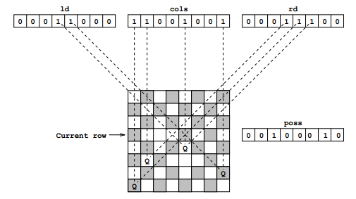
## References
- [Wikipedia](https://en.wikipedia.org/wiki/Eight_queens_puzzle)
- [GeeksForGeeks](https://www.geeksforgeeks.org/backtracking-set-3-n-queen-problem/)
- [On YouTube by Abdul Bari](https://www.youtube.com/watch?v=xFv_Hl4B83A&list=PLLXdhg_r2hKA7DPDsunoDZ-Z769jWn4R8)
- [On YouTube by Tushar Roy](https://www.youtube.com/watch?v=xouin83ebxE&list=PLLXdhg_r2hKA7DPDsunoDZ-Z769jWn4R8)
- Bitwise Solution
- [Wikipedia](https://en.wikipedia.org/wiki/Eight_queens_puzzle)
- [Solution by Greg Trowbridge](http://gregtrowbridge.com/a-bitwise-solution-to-the-n-queens-problem-in-javascript/)
================================================
FILE: src/algorithms/uncategorized/n-queens/__test__/QueensPosition.test.js
================================================
import QueenPosition from '../QueenPosition';
describe('QueenPosition', () => {
it('should store queen position on chessboard', () => {
const position1 = new QueenPosition(0, 0);
const position2 = new QueenPosition(2, 1);
expect(position2.columnIndex).toBe(1);
expect(position2.rowIndex).toBe(2);
expect(position1.leftDiagonal).toBe(0);
expect(position1.rightDiagonal).toBe(0);
expect(position2.leftDiagonal).toBe(1);
expect(position2.rightDiagonal).toBe(3);
expect(position2.toString()).toBe('2,1');
});
});
================================================
FILE: src/algorithms/uncategorized/n-queens/__test__/nQueens.test.js
================================================
import nQueens from '../nQueens';
describe('nQueens', () => {
it('should not hae solution for 3 queens', () => {
const solutions = nQueens(3);
expect(solutions.length).toBe(0);
});
it('should solve n-queens problem for 4 queens', () => {
const solutions = nQueens(4);
expect(solutions.length).toBe(2);
// First solution.
expect(solutions[0][0].toString()).toBe('0,1');
expect(solutions[0][1].toString()).toBe('1,3');
expect(solutions[0][2].toString()).toBe('2,0');
expect(solutions[0][3].toString()).toBe('3,2');
// Second solution (mirrored).
expect(solutions[1][0].toString()).toBe('0,2');
expect(solutions[1][1].toString()).toBe('1,0');
expect(solutions[1][2].toString()).toBe('2,3');
expect(solutions[1][3].toString()).toBe('3,1');
});
it('should solve n-queens problem for 6 queens', () => {
const solutions = nQueens(6);
expect(solutions.length).toBe(4);
// First solution.
expect(solutions[0][0].toString()).toBe('0,1');
expect(solutions[0][1].toString()).toBe('1,3');
expect(solutions[0][2].toString()).toBe('2,5');
expect(solutions[0][3].toString()).toBe('3,0');
expect(solutions[0][4].toString()).toBe('4,2');
expect(solutions[0][5].toString()).toBe('5,4');
});
});
================================================
FILE: src/algorithms/uncategorized/n-queens/__test__/nQueensBitwise.test.js
================================================
import nQueensBitwise from '../nQueensBitwise';
describe('nQueensBitwise', () => {
it('should have solutions for 4 to N queens', () => {
expect(nQueensBitwise(4)).toBe(2);
expect(nQueensBitwise(5)).toBe(10);
expect(nQueensBitwise(6)).toBe(4);
expect(nQueensBitwise(7)).toBe(40);
expect(nQueensBitwise(8)).toBe(92);
expect(nQueensBitwise(9)).toBe(352);
expect(nQueensBitwise(10)).toBe(724);
expect(nQueensBitwise(11)).toBe(2680);
});
});
================================================
FILE: src/algorithms/uncategorized/n-queens/nQueens.js
================================================
import QueenPosition from './QueenPosition';
/**
* @param {QueenPosition[]} queensPositions
* @param {number} rowIndex
* @param {number} columnIndex
* @return {boolean}
*/
function isSafe(queensPositions, rowIndex, columnIndex) {
// New position to which the Queen is going to be placed.
const newQueenPosition = new QueenPosition(rowIndex, columnIndex);
// Check if new queen position conflicts with any other queens.
for (let queenIndex = 0; queenIndex < queensPositions.length; queenIndex += 1) {
const currentQueenPosition = queensPositions[queenIndex];
if (
// Check if queen has been already placed.
currentQueenPosition
&& (
// Check if there are any queen on the same column.
newQueenPosition.columnIndex === currentQueenPosition.columnIndex
// Check if there are any queen on the same row.
|| newQueenPosition.rowIndex === currentQueenPosition.rowIndex
// Check if there are any queen on the same left diagonal.
|| newQueenPosition.leftDiagonal === currentQueenPosition.leftDiagonal
// Check if there are any queen on the same right diagonal.
|| newQueenPosition.rightDiagonal === currentQueenPosition.rightDiagonal
)
) {
// Can't place queen into current position since there are other queens that
// are threatening it.
return false;
}
}
// Looks like we're safe.
return true;
}
/**
* @param {QueenPosition[][]} solutions
* @param {QueenPosition[]} previousQueensPositions
* @param {number} queensCount
* @param {number} rowIndex
* @return {boolean}
*/
function nQueensRecursive(solutions, previousQueensPositions, queensCount, rowIndex) {
// Clone positions array.
const queensPositions = [...previousQueensPositions].map((queenPosition) => {
return !queenPosition ? queenPosition : new QueenPosition(
queenPosition.rowIndex,
queenPosition.columnIndex,
);
});
if (rowIndex === queensCount) {
// We've successfully reached the end of the board.
// Store solution to the list of solutions.
solutions.push(queensPositions);
// Solution found.
return true;
}
// Let's try to put queen at row rowIndex into its safe column position.
for (let columnIndex = 0; columnIndex < queensCount; columnIndex += 1) {
if (isSafe(queensPositions, rowIndex, columnIndex)) {
// Place current queen to its current position.
queensPositions[rowIndex] = new QueenPosition(rowIndex, columnIndex);
// Try to place all other queens as well.
nQueensRecursive(solutions, queensPositions, queensCount, rowIndex + 1);
// BACKTRACKING.
// Remove the queen from the row to avoid isSafe() returning false.
queensPositions[rowIndex] = null;
}
}
return false;
}
/**
* @param {number} queensCount
* @return {QueenPosition[][]}
*/
export default function nQueens(queensCount) {
// Init NxN chessboard with zeros.
// const chessboard = Array(queensCount).fill(null).map(() => Array(queensCount).fill(0));
// This array will hold positions or coordinates of each of
// N queens in form of [rowIndex, columnIndex].
const queensPositions = Array(queensCount).fill(null);
/** @var {QueenPosition[][]} solutions */
const solutions = [];
// Solve problem recursively.
nQueensRecursive(solutions, queensPositions, queensCount, 0);
return solutions;
}
================================================
FILE: src/algorithms/uncategorized/n-queens/nQueensBitwise.js
================================================
/**
* Checks all possible board configurations.
*
* @param {number} boardSize - Size of the squared chess board.
* @param {number} leftDiagonal - Sequence of N bits that show whether the corresponding location
* on the current row is "available" (no other queens are threatening from left diagonal).
* @param {number} column - Sequence of N bits that show whether the corresponding location
* on the current row is "available" (no other queens are threatening from columns).
* @param {number} rightDiagonal - Sequence of N bits that show whether the corresponding location
* on the current row is "available" (no other queens are threatening from right diagonal).
* @param {number} solutionsCount - Keeps track of the number of valid solutions.
* @return {number} - Number of possible solutions.
*/
function nQueensBitwiseRecursive(
boardSize,
leftDiagonal = 0,
column = 0,
rightDiagonal = 0,
solutionsCount = 0,
) {
// Keeps track of the number of valid solutions.
let currentSolutionsCount = solutionsCount;
// Helps to identify valid solutions.
// isDone simply has a bit sequence with 1 for every entry up to the Nth. For example,
// when N=5, done will equal 11111. The "isDone" variable simply allows us to not worry about any
// bits beyond the Nth.
const isDone = (2 ** boardSize) - 1;
// All columns are occupied (i.e. 0b1111 for boardSize = 4), so the solution must be complete.
// Since the algorithm never places a queen illegally (ie. when it can attack or be attacked),
// we know that if all the columns have been filled, we must have a valid solution.
if (column === isDone) {
return currentSolutionsCount + 1;
}
// Gets a bit sequence with "1"s wherever there is an open "slot".
// All that's happening here is we're taking col, ld, and rd, and if any of the columns are
// "under attack", we mark that column as 0 in poss, basically meaning "we can't put a queen in
// this column". Thus all bits position in poss that are '1's are available for placing
// queen there.
let availablePositions = ~(leftDiagonal | rightDiagonal | column);
// Loops as long as there is a valid place to put another queen.
// For N=4 the isDone=0b1111. Then if availablePositions=0b0000 (which would mean that all places
// are under threatening) we must stop trying to place a queen.
while (availablePositions & isDone) {
// firstAvailablePosition just stores the first non-zero bit (ie. the first available location).
// So if firstAvailablePosition was 0010, it would mean the 3rd column of the current row.
// And that would be the position will be placing our next queen.
//
// For example:
// availablePositions = 0b01100
// firstAvailablePosition = 100
const firstAvailablePosition = availablePositions & -availablePositions;
// This line just marks that position in the current row as being "taken" by flipping that
// column in availablePositions to zero. This way, when the while loop continues, we'll know
// not to try that location again.
//
// For example:
// availablePositions = 0b0100
// firstAvailablePosition = 0b10
// 0b0110 - 0b10 = 0b0100
availablePositions -= firstAvailablePosition;
/*
* The operators >> 1 and 1 << simply move all the bits in a bit sequence one digit to the
* right or left, respectively. So calling (rd|bit)<<1 simply says: combine rd and bit with
* an OR operation, then move everything in the result to the left by one digit.
*
* More specifically, if rd is 0001 (meaning that the top-right-to-bottom-left diagonal through
* column 4 of the current row is occupied), and bit is 0100 (meaning that we are planning to
* place a queen in column 2 of the current row), (rd|bit) results in 0101 (meaning that after
* we place a queen in column 2 of the current row, the second and the fourth
* top-right-to-bottom-left diagonals will be occupied).
*
* Now, if add in the << operator, we get (rd|bit)<<1, which takes the 0101 we worked out in
* our previous bullet point, and moves everything to the left by one. The result, therefore,
* is 1010.
*/
currentSolutionsCount += nQueensBitwiseRecursive(
boardSize,
(leftDiagonal | firstAvailablePosition) >> 1,
column | firstAvailablePosition,
(rightDiagonal | firstAvailablePosition) << 1,
solutionsCount,
);
}
return currentSolutionsCount;
}
/**
* @param {number} boardSize - Size of the squared chess board.
* @return {number} - Number of possible solutions.
* @see http://gregtrowbridge.com/a-bitwise-solution-to-the-n-queens-problem-in-javascript/
*/
export default function nQueensBitwise(boardSize) {
return nQueensBitwiseRecursive(boardSize);
}
================================================
FILE: src/algorithms/uncategorized/rain-terraces/README.md
================================================
# Rain Terraces (Trapping Rain Water) Problem
Given an array of non-negative integers representing terraces in an elevation map
where the width of each bar is `1`, compute how much water it is able to trap
after raining.

## Examples
**Example #1**
```
Input: arr[] = [2, 0, 2]
Output: 2
Structure is like below:
| |
|_|
We can trap 2 units of water in the middle gap.
```
**Example #2**
```
Input: arr[] = [3, 0, 0, 2, 0, 4]
Output: 10
Structure is like below:
|
| |
| | |
|__|_|
We can trap "3*2 units" of water between 3 an 2,
"1 unit" on top of bar 2 and "3 units" between 2
and 4. See below diagram also.
```
**Example #3**
```
Input: arr[] = [0, 1, 0, 2, 1, 0, 1, 3, 2, 1, 2, 1]
Output: 6
Structure is like below:
|
| || |
_|_||_||||||
Trap "1 unit" between first 1 and 2, "4 units" between
first 2 and 3 and "1 unit" between second last 1 and last 2.
```
## The Algorithm
An element of array can store water if there are higher bars on left and right.
We can find amount of water to be stored in every element by finding the heights
of bars on left and right sides. The idea is to compute amount of water that can
be stored in every element of array. For example, consider the array
`[3, 0, 0, 2, 0, 4]`, We can trap "3*2 units" of water between 3 an 2, "1 unit"
on top of bar 2 and "3 units" between 2 and 4. See below diagram also.
### Approach 1: Brute force
**Intuition**
For each element in the array, we find the maximum level of water it can trap
after the rain, which is equal to the minimum of maximum height of bars on both
the sides minus its own height.
**Steps**
- Initialize `answer = 0`
- Iterate the array from left to right:
- Initialize `max_left = 0` and `max_right = 0`
- Iterate from the current element to the beginning of array updating: `max_left = max(max_left, height[j])`
- Iterate from the current element to the end of array updating: `max_right = max(max_right, height[j])`
- Add `min(max_left, max_right) − height[i]` to `answer`
**Complexity Analysis**
Time complexity: `O(n^2)`. For each element of array, we iterate the left and right parts.
Auxiliary space complexity: `O(1)` extra space.
### Approach 2: Dynamic Programming
**Intuition**
In brute force, we iterate over the left and right parts again and again just to
find the highest bar size up to that index. But, this could be stored. Voila,
dynamic programming.
So we may pre-compute highest bar on left and right of every bar in `O(n)` time.
Then use these pre-computed values to find the amount of water in every array element.
The concept is illustrated as shown:
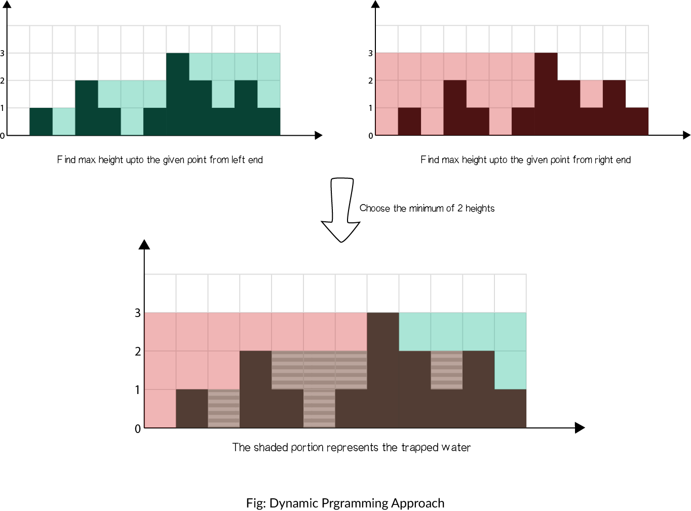
**Steps**
- Find maximum height of bar from the left end up to an index `i` in the array `left_max`.
- Find maximum height of bar from the right end up to an index `i` in the array `right_max`.
- Iterate over the `height` array and update `answer`:
- Add `min(max_left[i], max_right[i]) − height[i]` to `answer`.
**Complexity Analysis**
Time complexity: `O(n)`. We store the maximum heights upto a point using 2
iterations of `O(n)` each. We finally update `answer` using the stored
values in `O(n)`.
Auxiliary space complexity: `O(n)` extra space. Additional space
for `left_max` and `right_max` arrays than in Approach 1.
## References
- [GeeksForGeeks](https://www.geeksforgeeks.org/trapping-rain-water/)
- [LeetCode](https://leetcode.com/problems/trapping-rain-water/solution/)
================================================
FILE: src/algorithms/uncategorized/rain-terraces/__test__/bfRainTerraces.test.js
================================================
import bfRainTerraces from '../bfRainTerraces';
describe('bfRainTerraces', () => {
it('should find the amount of water collected after raining', () => {
expect(bfRainTerraces([1])).toBe(0);
expect(bfRainTerraces([1, 0])).toBe(0);
expect(bfRainTerraces([0, 1])).toBe(0);
expect(bfRainTerraces([0, 1, 0])).toBe(0);
expect(bfRainTerraces([0, 1, 0, 0])).toBe(0);
expect(bfRainTerraces([0, 1, 0, 0, 1, 0])).toBe(2);
expect(bfRainTerraces([0, 2, 0, 0, 1, 0])).toBe(2);
expect(bfRainTerraces([2, 0, 2])).toBe(2);
expect(bfRainTerraces([2, 0, 5])).toBe(2);
expect(bfRainTerraces([3, 0, 0, 2, 0, 4])).toBe(10);
expect(bfRainTerraces([0, 1, 0, 2, 1, 0, 1, 3, 2, 1, 2, 1])).toBe(6);
expect(bfRainTerraces([1, 1, 1, 1, 1])).toBe(0);
expect(bfRainTerraces([1, 2, 3, 4, 5])).toBe(0);
expect(bfRainTerraces([4, 1, 3, 1, 2, 1, 2, 1])).toBe(4);
expect(bfRainTerraces([0, 2, 4, 3, 4, 2, 4, 0, 8, 7, 0])).toBe(7);
});
});
================================================
FILE: src/algorithms/uncategorized/rain-terraces/__test__/dpRainTerraces.test.js
================================================
import dpRainTerraces from '../dpRainTerraces';
describe('dpRainTerraces', () => {
it('should find the amount of water collected after raining', () => {
expect(dpRainTerraces([1])).toBe(0);
expect(dpRainTerraces([1, 0])).toBe(0);
expect(dpRainTerraces([0, 1])).toBe(0);
expect(dpRainTerraces([0, 1, 0])).toBe(0);
expect(dpRainTerraces([0, 1, 0, 0])).toBe(0);
expect(dpRainTerraces([0, 1, 0, 0, 1, 0])).toBe(2);
expect(dpRainTerraces([0, 2, 0, 0, 1, 0])).toBe(2);
expect(dpRainTerraces([2, 0, 2])).toBe(2);
expect(dpRainTerraces([2, 0, 5])).toBe(2);
expect(dpRainTerraces([3, 0, 0, 2, 0, 4])).toBe(10);
expect(dpRainTerraces([0, 1, 0, 2, 1, 0, 1, 3, 2, 1, 2, 1])).toBe(6);
expect(dpRainTerraces([1, 1, 1, 1, 1])).toBe(0);
expect(dpRainTerraces([1, 2, 3, 4, 5])).toBe(0);
expect(dpRainTerraces([4, 1, 3, 1, 2, 1, 2, 1])).toBe(4);
expect(dpRainTerraces([0, 2, 4, 3, 4, 2, 4, 0, 8, 7, 0])).toBe(7);
});
});
================================================
FILE: src/algorithms/uncategorized/rain-terraces/bfRainTerraces.js
================================================
/**
* BRUTE FORCE approach of solving Trapping Rain Water problem.
*
* @param {number[]} terraces
* @return {number}
*/
export default function bfRainTerraces(terraces) {
let waterAmount = 0;
for (let terraceIndex = 0; terraceIndex < terraces.length; terraceIndex += 1) {
// Get left most high terrace.
let leftHighestLevel = 0;
for (let leftIndex = terraceIndex - 1; leftIndex >= 0; leftIndex -= 1) {
leftHighestLevel = Math.max(leftHighestLevel, terraces[leftIndex]);
}
// Get right most high terrace.
let rightHighestLevel = 0;
for (let rightIndex = terraceIndex + 1; rightIndex < terraces.length; rightIndex += 1) {
rightHighestLevel = Math.max(rightHighestLevel, terraces[rightIndex]);
}
// Add current terrace water amount.
const terraceBoundaryLevel = Math.min(leftHighestLevel, rightHighestLevel);
if (terraceBoundaryLevel > terraces[terraceIndex]) {
// Terrace will be able to store the water if the lowest of two left and right highest
// terraces are still higher than the current one.
waterAmount += terraceBoundaryLevel - terraces[terraceIndex];
}
}
return waterAmount;
}
================================================
FILE: src/algorithms/uncategorized/rain-terraces/dpRainTerraces.js
================================================
/**
* DYNAMIC PROGRAMMING approach of solving Trapping Rain Water problem.
*
* @param {number[]} terraces
* @return {number}
*/
export default function dpRainTerraces(terraces) {
let waterAmount = 0;
// Init arrays that will keep the list of left and right maximum levels for specific positions.
const leftMaxLevels = new Array(terraces.length).fill(0);
const rightMaxLevels = new Array(terraces.length).fill(0);
// Calculate the highest terrace level from the LEFT relative to the current terrace.
[leftMaxLevels[0]] = terraces;
for (let terraceIndex = 1; terraceIndex < terraces.length; terraceIndex += 1) {
leftMaxLevels[terraceIndex] = Math.max(
terraces[terraceIndex],
leftMaxLevels[terraceIndex - 1],
);
}
// Calculate the highest terrace level from the RIGHT relative to the current terrace.
rightMaxLevels[terraces.length - 1] = terraces[terraces.length - 1];
for (let terraceIndex = terraces.length - 2; terraceIndex >= 0; terraceIndex -= 1) {
rightMaxLevels[terraceIndex] = Math.max(
terraces[terraceIndex],
rightMaxLevels[terraceIndex + 1],
);
}
// Not let's go through all terraces one by one and calculate how much water
// each terrace may accumulate based on previously calculated values.
for (let terraceIndex = 0; terraceIndex < terraces.length; terraceIndex += 1) {
// Pick the lowest from the left/right highest terraces.
const currentTerraceBoundary = Math.min(
leftMaxLevels[terraceIndex],
rightMaxLevels[terraceIndex],
);
if (currentTerraceBoundary > terraces[terraceIndex]) {
waterAmount += currentTerraceBoundary - terraces[terraceIndex];
}
}
return waterAmount;
}
================================================
FILE: src/algorithms/uncategorized/recursive-staircase/README.md
================================================
# Recursive Staircase Problem
## The Problem
There are `n` stairs, a person standing at the bottom wants to reach the top. The person can climb either `1` or `2` stairs at a time. _Count the number of ways, the person can reach the top._

## The Solution
This is an interesting problem because there are several ways of how it may be solved that illustrate different programming paradigms.
- [Brute Force Recursive Solution](./recursiveStaircaseBF.js) - Time: `O(2^n)`; Space: `O(1)`
- [Recursive Solution With Memoization](./recursiveStaircaseMEM.js) - Time: `O(n)`; Space: `O(n)`
- [Dynamic Programming Solution](./recursiveStaircaseDP.js) - Time: `O(n)`; Space: `O(n)`
- [Iterative Solution](./recursiveStaircaseIT.js) - Time: `O(n)`; Space: `O(1)`
## References
- [On YouTube by Gayle Laakmann McDowell](https://www.youtube.com/watch?v=eREiwuvzaUM&list=PLLXdhg_r2hKA7DPDsunoDZ-Z769jWn4R8&index=81&t=0s)
- [GeeksForGeeks](https://www.geeksforgeeks.org/count-ways-reach-nth-stair/)
================================================
FILE: src/algorithms/uncategorized/recursive-staircase/__test__/recursiveStaircaseBF.test.js
================================================
import recursiveStaircaseBF from '../recursiveStaircaseBF';
describe('recursiveStaircaseBF', () => {
it('should calculate number of variants using Brute Force solution', () => {
expect(recursiveStaircaseBF(-1)).toBe(0);
expect(recursiveStaircaseBF(0)).toBe(0);
expect(recursiveStaircaseBF(1)).toBe(1);
expect(recursiveStaircaseBF(2)).toBe(2);
expect(recursiveStaircaseBF(3)).toBe(3);
expect(recursiveStaircaseBF(4)).toBe(5);
expect(recursiveStaircaseBF(5)).toBe(8);
expect(recursiveStaircaseBF(6)).toBe(13);
expect(recursiveStaircaseBF(7)).toBe(21);
expect(recursiveStaircaseBF(8)).toBe(34);
expect(recursiveStaircaseBF(9)).toBe(55);
expect(recursiveStaircaseBF(10)).toBe(89);
});
});
================================================
FILE: src/algorithms/uncategorized/recursive-staircase/__test__/recursiveStaircaseDP.test.js
================================================
import recursiveStaircaseDP from '../recursiveStaircaseDP';
describe('recursiveStaircaseDP', () => {
it('should calculate number of variants using Dynamic Programming solution', () => {
expect(recursiveStaircaseDP(-1)).toBe(0);
expect(recursiveStaircaseDP(0)).toBe(0);
expect(recursiveStaircaseDP(1)).toBe(1);
expect(recursiveStaircaseDP(2)).toBe(2);
expect(recursiveStaircaseDP(3)).toBe(3);
expect(recursiveStaircaseDP(4)).toBe(5);
expect(recursiveStaircaseDP(5)).toBe(8);
expect(recursiveStaircaseDP(6)).toBe(13);
expect(recursiveStaircaseDP(7)).toBe(21);
expect(recursiveStaircaseDP(8)).toBe(34);
expect(recursiveStaircaseDP(9)).toBe(55);
expect(recursiveStaircaseDP(10)).toBe(89);
});
});
================================================
FILE: src/algorithms/uncategorized/recursive-staircase/__test__/recursiveStaircaseIT.test.js
================================================
import recursiveStaircaseIT from '../recursiveStaircaseIT';
describe('recursiveStaircaseIT', () => {
it('should calculate number of variants using Iterative solution', () => {
expect(recursiveStaircaseIT(-1)).toBe(0);
expect(recursiveStaircaseIT(0)).toBe(0);
expect(recursiveStaircaseIT(1)).toBe(1);
expect(recursiveStaircaseIT(2)).toBe(2);
expect(recursiveStaircaseIT(3)).toBe(3);
expect(recursiveStaircaseIT(4)).toBe(5);
expect(recursiveStaircaseIT(5)).toBe(8);
expect(recursiveStaircaseIT(6)).toBe(13);
expect(recursiveStaircaseIT(7)).toBe(21);
expect(recursiveStaircaseIT(8)).toBe(34);
expect(recursiveStaircaseIT(9)).toBe(55);
expect(recursiveStaircaseIT(10)).toBe(89);
});
});
================================================
FILE: src/algorithms/uncategorized/recursive-staircase/__test__/recursiveStaircaseMEM.test.js
================================================
import recursiveStaircaseMEM from '../recursiveStaircaseMEM';
describe('recursiveStaircaseMEM', () => {
it('should calculate number of variants using Brute Force with Memoization', () => {
expect(recursiveStaircaseMEM(-1)).toBe(0);
expect(recursiveStaircaseMEM(0)).toBe(0);
expect(recursiveStaircaseMEM(1)).toBe(1);
expect(recursiveStaircaseMEM(2)).toBe(2);
expect(recursiveStaircaseMEM(3)).toBe(3);
expect(recursiveStaircaseMEM(4)).toBe(5);
expect(recursiveStaircaseMEM(5)).toBe(8);
expect(recursiveStaircaseMEM(6)).toBe(13);
expect(recursiveStaircaseMEM(7)).toBe(21);
expect(recursiveStaircaseMEM(8)).toBe(34);
expect(recursiveStaircaseMEM(9)).toBe(55);
expect(recursiveStaircaseMEM(10)).toBe(89);
});
});
================================================
FILE: src/algorithms/uncategorized/recursive-staircase/recursiveStaircaseBF.js
================================================
/**
* Recursive Staircase Problem (Brute Force Solution).
*
* @param {number} stairsNum - Number of stairs to climb on.
* @return {number} - Number of ways to climb a staircase.
*/
export default function recursiveStaircaseBF(stairsNum) {
if (stairsNum <= 0) {
// There is no way to go down - you climb the stairs only upwards.
// Also if you're standing on the ground floor that you don't need to do any further steps.
return 0;
}
if (stairsNum === 1) {
// There is only one way to go to the first step.
return 1;
}
if (stairsNum === 2) {
// There are two ways to get to the second steps: (1 + 1) or (2).
return 2;
}
// Sum up how many steps we need to take after doing one step up with the number of
// steps we need to take after doing two steps up.
return recursiveStaircaseBF(stairsNum - 1) + recursiveStaircaseBF(stairsNum - 2);
}
================================================
FILE: src/algorithms/uncategorized/recursive-staircase/recursiveStaircaseDP.js
================================================
/**
* Recursive Staircase Problem (Dynamic Programming Solution).
*
* @param {number} stairsNum - Number of stairs to climb on.
* @return {number} - Number of ways to climb a staircase.
*/
export default function recursiveStaircaseDP(stairsNum) {
if (stairsNum < 0) {
// There is no way to go down - you climb the stairs only upwards.
return 0;
}
// Init the steps vector that will hold all possible ways to get to the corresponding step.
const steps = new Array(stairsNum + 1).fill(0);
// Init the number of ways to get to the 0th, 1st and 2nd steps.
steps[0] = 0;
steps[1] = 1;
steps[2] = 2;
if (stairsNum <= 2) {
// Return the number of ways to get to the 0th or 1st or 2nd steps.
return steps[stairsNum];
}
// Calculate every next step based on two previous ones.
for (let currentStep = 3; currentStep <= stairsNum; currentStep += 1) {
steps[currentStep] = steps[currentStep - 1] + steps[currentStep - 2];
}
// Return possible ways to get to the requested step.
return steps[stairsNum];
}
================================================
FILE: src/algorithms/uncategorized/recursive-staircase/recursiveStaircaseIT.js
================================================
/**
* Recursive Staircase Problem (Iterative Solution).
*
* @param {number} stairsNum - Number of stairs to climb on.
* @return {number} - Number of ways to climb a staircase.
*/
export default function recursiveStaircaseIT(stairsNum) {
if (stairsNum <= 0) {
// There is no way to go down - you climb the stairs only upwards.
// Also you don't need to do anything to stay on the 0th step.
return 0;
}
// Init the number of ways to get to the 0th, 1st and 2nd steps.
const steps = [1, 2];
if (stairsNum <= 2) {
// Return the number of possible ways of how to get to the 1st or 2nd steps.
return steps[stairsNum - 1];
}
// Calculate the number of ways to get to the n'th step based on previous ones.
// Comparing to Dynamic Programming solution we don't store info for all the steps but
// rather for two previous ones only.
for (let currentStep = 3; currentStep <= stairsNum; currentStep += 1) {
[steps[0], steps[1]] = [steps[1], steps[0] + steps[1]];
}
// Return possible ways to get to the requested step.
return steps[1];
}
================================================
FILE: src/algorithms/uncategorized/recursive-staircase/recursiveStaircaseMEM.js
================================================
/**
* Recursive Staircase Problem (Recursive Solution With Memoization).
*
* @param {number} totalStairs - Number of stairs to climb on.
* @return {number} - Number of ways to climb a staircase.
*/
export default function recursiveStaircaseMEM(totalStairs) {
// Memo table that will hold all recursively calculated results to avoid calculating them
// over and over again.
const memo = [];
// Recursive closure.
const getSteps = (stairsNum) => {
if (stairsNum <= 0) {
// There is no way to go down - you climb the stairs only upwards.
// Also if you're standing on the ground floor that you don't need to do any further steps.
return 0;
}
if (stairsNum === 1) {
// There is only one way to go to the first step.
return 1;
}
if (stairsNum === 2) {
// There are two ways to get to the second steps: (1 + 1) or (2).
return 2;
}
// Avoid recursion for the steps that we've calculated recently.
if (memo[stairsNum]) {
return memo[stairsNum];
}
// Sum up how many steps we need to take after doing one step up with the number of
// steps we need to take after doing two steps up.
memo[stairsNum] = getSteps(stairsNum - 1) + getSteps(stairsNum - 2);
return memo[stairsNum];
};
// Return possible ways to get to the requested step.
return getSteps(totalStairs);
}
================================================
FILE: src/algorithms/uncategorized/square-matrix-rotation/README.md
================================================
# Square Matrix In-Place Rotation
## The Problem
You are given an `n x n` 2D matrix (representing an image).
Rotate the matrix by `90` degrees (clockwise).
**Note**
You have to rotate the image **in-place**, which means you
have to modify the input 2D matrix directly. **DO NOT** allocate
another 2D matrix and do the rotation.
## Examples
**Example #1**
Given input matrix:
```
[
[1, 2, 3],
[4, 5, 6],
[7, 8, 9],
]
```
Rotate the input matrix in-place such that it becomes:
```
[
[7, 4, 1],
[8, 5, 2],
[9, 6, 3],
]
```
**Example #2**
Given input matrix:
```
[
[5, 1, 9, 11],
[2, 4, 8, 10],
[13, 3, 6, 7],
[15, 14, 12, 16],
]
```
Rotate the input matrix in-place such that it becomes:
```
[
[15, 13, 2, 5],
[14, 3, 4, 1],
[12, 6, 8, 9],
[16, 7, 10, 11],
]
```
## Algorithm
We would need to do two reflections of the matrix:
- reflect vertically
- reflect diagonally from bottom-left to top-right
Or we also could Furthermore, you can reflect diagonally
top-left/bottom-right and reflect horizontally.
A common question is how do you even figure out what kind
of reflections to do? Simply rip a square piece of paper,
write a random word on it so you know its rotation. Then,
flip the square piece of paper around until you figure out
how to come to the solution.
Here is an example of how first line may be rotated using
diagonal top-right/bottom-left rotation along with horizontal
rotation.
```
Let's say we have a string at the top of the matrix:
A B C
• • •
• • •
Let's do top-right/bottom-left diagonal reflection:
A B C
/ / •
/ • •
And now let's do horizontal reflection:
A → →
B → →
C → →
The string has been rotated to 90 degree:
• • A
• • B
• • C
```
## References
- [LeetCode](https://leetcode.com/problems/rotate-image/description/)
================================================
FILE: src/algorithms/uncategorized/square-matrix-rotation/__test__/squareMatrixRotation.test.js
================================================
import squareMatrixRotation from '../squareMatrixRotation';
describe('squareMatrixRotation', () => {
it('should rotate matrix #0 in-place', () => {
const matrix = [[1]];
const rotatedMatrix = [[1]];
expect(squareMatrixRotation(matrix)).toEqual(rotatedMatrix);
});
it('should rotate matrix #1 in-place', () => {
const matrix = [
[1, 2],
[3, 4],
];
const rotatedMatrix = [
[3, 1],
[4, 2],
];
expect(squareMatrixRotation(matrix)).toEqual(rotatedMatrix);
});
it('should rotate matrix #2 in-place', () => {
const matrix = [
[1, 2, 3],
[4, 5, 6],
[7, 8, 9],
];
const rotatedMatrix = [
[7, 4, 1],
[8, 5, 2],
[9, 6, 3],
];
expect(squareMatrixRotation(matrix)).toEqual(rotatedMatrix);
});
it('should rotate matrix #3 in-place', () => {
const matrix = [
[5, 1, 9, 11],
[2, 4, 8, 10],
[13, 3, 6, 7],
[15, 14, 12, 16],
];
const rotatedMatrix = [
[15, 13, 2, 5],
[14, 3, 4, 1],
[12, 6, 8, 9],
[16, 7, 10, 11],
];
expect(squareMatrixRotation(matrix)).toEqual(rotatedMatrix);
});
});
================================================
FILE: src/algorithms/uncategorized/square-matrix-rotation/squareMatrixRotation.js
================================================
/**
* @param {*[][]} originalMatrix
* @return {*[][]}
*/
export default function squareMatrixRotation(originalMatrix) {
const matrix = originalMatrix.slice();
// Do top-right/bottom-left diagonal reflection of the matrix.
for (let rowIndex = 0; rowIndex < matrix.length; rowIndex += 1) {
for (let columnIndex = rowIndex + 1; columnIndex < matrix.length; columnIndex += 1) {
// Swap elements.
[
matrix[columnIndex][rowIndex],
matrix[rowIndex][columnIndex],
] = [
matrix[rowIndex][columnIndex],
matrix[columnIndex][rowIndex],
];
}
}
// Do horizontal reflection of the matrix.
for (let rowIndex = 0; rowIndex < matrix.length; rowIndex += 1) {
for (let columnIndex = 0; columnIndex < matrix.length / 2; columnIndex += 1) {
// Swap elements.
[
matrix[rowIndex][matrix.length - columnIndex - 1],
matrix[rowIndex][columnIndex],
] = [
matrix[rowIndex][columnIndex],
matrix[rowIndex][matrix.length - columnIndex - 1],
];
}
}
return matrix;
}
================================================
FILE: src/algorithms/uncategorized/unique-paths/README.md
================================================
# Unique Paths Problem
A robot is located at the top-left corner of a `m x n` grid
(marked 'Start' in the diagram below).
The robot can only move either down or right at any point in
time. The robot is trying to reach the bottom-right corner
of the grid (marked 'Finish' in the diagram below).
How many possible unique paths are there?

## Examples
**Example #1**
```
Input: m = 3, n = 2
Output: 3
Explanation:
From the top-left corner, there are a total of 3 ways to reach the bottom-right corner:
1. Right -> Right -> Down
2. Right -> Down -> Right
3. Down -> Right -> Right
```
**Example #2**
```
Input: m = 7, n = 3
Output: 28
```
## Algorithms
### Backtracking
First thought that might came to mind is that we need to build a decision tree
where `D` means moving down and `R` means moving right. For example in case
of boars `width = 3` and `height = 2` we will have the following decision tree:
```
START
/ \
D R
/ / \
R D R
/ / \
R R D
END END END
```
We can see three unique branches here that is the answer to our problem.
**Time Complexity**: `O(2 ^ n)` - roughly in worst case with square board
of size `n`.
**Auxiliary Space Complexity**: `O(m + n)` - since we need to store current path with
positions.
### Dynamic Programming
Let's treat `BOARD[i][j]` as our sub-problem.
Since we have restriction of moving only to the right
and down we might say that number of unique paths to the current
cell is a sum of numbers of unique paths to the cell above the
current one and to the cell to the left of current one.
```
BOARD[i][j] = BOARD[i - 1][j] + BOARD[i][j - 1]; // since we can only move down or right.
```
Base cases are:
```
BOARD[0][any] = 1; // only one way to reach any top slot.
BOARD[any][0] = 1; // only one way to reach any slot in the leftmost column.
```
For the board `3 x 2` our dynamic programming matrix will look like:
| | 0 | 1 | 1 |
|:---:|:---:|:---:|:---:|
|**0**| 0 | 1 | 1 |
|**1**| 1 | 2 | 3 |
Each cell contains the number of unique paths to it. We need
the bottom right one with number `3`.
**Time Complexity**: `O(m * n)` - since we're going through each cell of the DP matrix.
**Auxiliary Space Complexity**: `O(m * n)` - since we need to have DP matrix.
### Pascal's Triangle Based
This question is actually another form of Pascal Triangle.
The corner of this rectangle is at `m + n - 2` line, and
at `min(m, n) - 1` position of the Pascal's Triangle.
## References
- [LeetCode](https://leetcode.com/problems/unique-paths/description/)
================================================
FILE: src/algorithms/uncategorized/unique-paths/__test__/btUniquePaths.test.js
================================================
import btUniquePaths from '../btUniquePaths';
describe('btUniquePaths', () => {
it('should find the number of unique paths on board', () => {
expect(btUniquePaths(3, 2)).toBe(3);
expect(btUniquePaths(7, 3)).toBe(28);
expect(btUniquePaths(3, 7)).toBe(28);
expect(btUniquePaths(10, 10)).toBe(48620);
expect(btUniquePaths(100, 1)).toBe(1);
expect(btUniquePaths(1, 100)).toBe(1);
});
});
================================================
FILE: src/algorithms/uncategorized/unique-paths/__test__/dpUniquePaths.test.js
================================================
import dpUniquePaths from '../dpUniquePaths';
describe('dpUniquePaths', () => {
it('should find the number of unique paths on board', () => {
expect(dpUniquePaths(3, 2)).toBe(3);
expect(dpUniquePaths(7, 3)).toBe(28);
expect(dpUniquePaths(3, 7)).toBe(28);
expect(dpUniquePaths(10, 10)).toBe(48620);
expect(dpUniquePaths(100, 1)).toBe(1);
expect(dpUniquePaths(1, 100)).toBe(1);
});
});
================================================
FILE: src/algorithms/uncategorized/unique-paths/__test__/uniquePaths.test.js
================================================
import uniquePaths from '../uniquePaths';
describe('uniquePaths', () => {
it('should find the number of unique paths on board', () => {
expect(uniquePaths(3, 2)).toBe(3);
expect(uniquePaths(7, 3)).toBe(28);
expect(uniquePaths(3, 7)).toBe(28);
expect(uniquePaths(10, 10)).toBe(48620);
expect(uniquePaths(100, 1)).toBe(1);
expect(uniquePaths(1, 100)).toBe(1);
});
});
================================================
FILE: src/algorithms/uncategorized/unique-paths/btUniquePaths.js
================================================
/**
* BACKTRACKING approach of solving Unique Paths problem.
*
* @param {number} width - Width of the board.
* @param {number} height - Height of the board.
* @param {number[][]} steps - The steps that have been already made.
* @param {number} uniqueSteps - Total number of unique steps.
* @return {number} - Number of unique paths.
*/
export default function btUniquePaths(width, height, steps = [[0, 0]], uniqueSteps = 0) {
// Fetch current position on board.
const currentPos = steps[steps.length - 1];
// Check if we've reached the end.
if (currentPos[0] === width - 1 && currentPos[1] === height - 1) {
// In case if we've reached the end let's increase total
// number of unique steps.
return uniqueSteps + 1;
}
// Let's calculate how many unique path we will have
// by going right and by going down.
let rightUniqueSteps = 0;
let downUniqueSteps = 0;
// Do right step if possible.
if (currentPos[0] < width - 1) {
steps.push([
currentPos[0] + 1,
currentPos[1],
]);
// Calculate how many unique paths we'll get by moving right.
rightUniqueSteps = btUniquePaths(width, height, steps, uniqueSteps);
// BACKTRACK and try another move.
steps.pop();
}
// Do down step if possible.
if (currentPos[1] < height - 1) {
steps.push([
currentPos[0],
currentPos[1] + 1,
]);
// Calculate how many unique paths we'll get by moving down.
downUniqueSteps = btUniquePaths(width, height, steps, uniqueSteps);
// BACKTRACK and try another move.
steps.pop();
}
// Total amount of unique steps will be equal to total amount of
// unique steps by going right plus total amount of unique steps
// by going down.
return rightUniqueSteps + downUniqueSteps;
}
================================================
FILE: src/algorithms/uncategorized/unique-paths/dpUniquePaths.js
================================================
/**
* DYNAMIC PROGRAMMING approach of solving Unique Paths problem.
*
* @param {number} width - Width of the board.
* @param {number} height - Height of the board.
* @return {number} - Number of unique paths.
*/
export default function dpUniquePaths(width, height) {
// Init board.
const board = Array(height).fill(null).map(() => {
return Array(width).fill(0);
});
// Base case.
// There is only one way of getting to board[0][any] and
// there is also only one way of getting to board[any][0].
// This is because we have a restriction of moving right
// and down only.
for (let rowIndex = 0; rowIndex < height; rowIndex += 1) {
for (let columnIndex = 0; columnIndex < width; columnIndex += 1) {
if (rowIndex === 0 || columnIndex === 0) {
board[rowIndex][columnIndex] = 1;
}
}
}
// Now, since we have this restriction of moving only to the right
// and down we might say that number of unique paths to the current
// cell is a sum of numbers of unique paths to the cell above the
// current one and to the cell to the left of current one.
for (let rowIndex = 1; rowIndex < height; rowIndex += 1) {
for (let columnIndex = 1; columnIndex < width; columnIndex += 1) {
const uniquesFromTop = board[rowIndex - 1][columnIndex];
const uniquesFromLeft = board[rowIndex][columnIndex - 1];
board[rowIndex][columnIndex] = uniquesFromTop + uniquesFromLeft;
}
}
return board[height - 1][width - 1];
}
================================================
FILE: src/algorithms/uncategorized/unique-paths/uniquePaths.js
================================================
import pascalTriangle from '../../math/pascal-triangle/pascalTriangle';
/**
* @param {number} width
* @param {number} height
* @return {number}
*/
export default function uniquePaths(width, height) {
const pascalLine = width + height - 2;
const pascalLinePosition = Math.min(width, height) - 1;
return pascalTriangle(pascalLine)[pascalLinePosition];
}
================================================
FILE: src/data-structures/bloom-filter/BloomFilter.js
================================================
export default class BloomFilter {
/**
* @param {number} size - the size of the storage.
*/
constructor(size = 100) {
// Bloom filter size directly affects the likelihood of false positives.
// The bigger the size the lower the likelihood of false positives.
this.size = size;
this.storage = this.createStore(size);
}
/**
* @param {string} item
*/
insert(item) {
const hashValues = this.getHashValues(item);
// Set each hashValue index to true.
hashValues.forEach((val) => this.storage.setValue(val));
}
/**
* @param {string} item
* @return {boolean}
*/
mayContain(item) {
const hashValues = this.getHashValues(item);
for (let hashIndex = 0; hashIndex < hashValues.length; hashIndex += 1) {
if (!this.storage.getValue(hashValues[hashIndex])) {
// We know that the item was definitely not inserted.
return false;
}
}
// The item may or may not have been inserted.
return true;
}
/**
* Creates the data store for our filter.
* We use this method to generate the store in order to
* encapsulate the data itself and only provide access
* to the necessary methods.
*
* @param {number} size
* @return {Object}
*/
createStore(size) {
const storage = [];
// Initialize all indexes to false
for (let storageCellIndex = 0; storageCellIndex < size; storageCellIndex += 1) {
storage.push(false);
}
const storageInterface = {
getValue(index) {
return storage[index];
},
setValue(index) {
storage[index] = true;
},
};
return storageInterface;
}
/**
* @param {string} item
* @return {number}
*/
hash1(item) {
let hash = 0;
for (let charIndex = 0; charIndex < item.length; charIndex += 1) {
const char = item.charCodeAt(charIndex);
hash = (hash << 5) + hash + char;
hash &= hash; // Convert to 32bit integer
hash = Math.abs(hash);
}
return hash % this.size;
}
/**
* @param {string} item
* @return {number}
*/
hash2(item) {
let hash = 5381;
for (let charIndex = 0; charIndex < item.length; charIndex += 1) {
const char = item.charCodeAt(charIndex);
hash = (hash << 5) + hash + char; /* hash * 33 + c */
}
return Math.abs(hash % this.size);
}
/**
* @param {string} item
* @return {number}
*/
hash3(item) {
let hash = 0;
for (let charIndex = 0; charIndex < item.length; charIndex += 1) {
const char = item.charCodeAt(charIndex);
hash = (hash << 5) - hash;
hash += char;
hash &= hash; // Convert to 32bit integer
}
return Math.abs(hash % this.size);
}
/**
* Runs all 3 hash functions on the input and returns an array of results.
*
* @param {string} item
* @return {number[]}
*/
getHashValues(item) {
return [
this.hash1(item),
this.hash2(item),
this.hash3(item),
];
}
}
================================================
FILE: src/data-structures/bloom-filter/README.md
================================================
# Bloom Filter
_Read this in other languages:_
[_Русский_](README.ru-RU.md),
[_Português_](README.pt-BR.md),
[_Українська_](README.uk-UA.md)
A **bloom filter** is a space-efficient probabilistic
data structure designed to test whether an element
is present in a set. It is designed to be blazingly
fast and use minimal memory at the cost of potential
false positives. False positive matches are possible,
but false negatives are not – in other words, a query
returns either "possibly in set" or "definitely not in set".
Bloom proposed the technique for applications where the
amount of source data would require an impractically large
amount of memory if "conventional" error-free hashing
techniques were applied.
## Algorithm description
An empty Bloom filter is a bit array of `m` bits, all
set to `0`. There must also be `k` different hash functions
defined, each of which maps or hashes some set element to
one of the `m` array positions, generating a uniform random
distribution. Typically, `k` is a constant, much smaller
than `m`, which is proportional to the number of elements
to be added; the precise choice of `k` and the constant of
proportionality of `m` are determined by the intended
false positive rate of the filter.
Here is an example of a Bloom filter, representing the
set `{x, y, z}`. The colored arrows show the positions
in the bit array that each set element is mapped to. The
element `w` is not in the set `{x, y, z}`, because it
hashes to one bit-array position containing `0`. For
this figure, `m = 18` and `k = 3`.

## Operations
There are two main operations a bloom filter can
perform: _insertion_ and _search_. Search may result in
false positives. Deletion is not possible.
In other words, the filter can take in items. When
we go to check if an item has previously been
inserted, it can tell us either "no" or "maybe".
Both insertion and search are `O(1)` operations.
## Making the filter
A bloom filter is created by allotting a certain size.
In our example, we use `100` as a default length. All
locations are initialized to `false`.
### Insertion
During insertion, a number of hash functions,
in our case `3` hash functions, are used to create
hashes of the input. These hash functions output
indexes. At every index received, we simply change
the value in our bloom filter to `true`.
### Search
During a search, the same hash functions are called
and used to hash the input. We then check if the
indexes received _all_ have a value of `true` inside
our bloom filter. If they _all_ have a value of
`true`, we know that the bloom filter may have had
the value previously inserted.
However, it's not certain, because it's possible
that other values previously inserted flipped the
values to `true`. The values aren't necessarily
`true` due to the item currently being searched for.
Absolute certainty is impossible unless only a single
item has previously been inserted.
While checking the bloom filter for the indexes
returned by our hash functions, if even one of them
has a value of `false`, we definitively know that the
item was not previously inserted.
## False Positives
The probability of false positives is determined by
three factors: the size of the bloom filter, the
number of hash functions we use, and the number
of items that have been inserted into the filter.
The formula to calculate probability of a false positive is:
( 1 - e -kn/m ) k
`k` = number of hash functions
`m` = filter size
`n` = number of items inserted
These variables, `k`, `m`, and `n`, should be picked based
on how acceptable false positives are. If the values
are picked and the resulting probability is too high,
the values should be tweaked and the probability
re-calculated.
## Applications
A bloom filter can be used on a blogging website. If
the goal is to show readers only articles that they
have never seen before, a bloom filter is perfect.
It can store hashed values based on the articles. After
a user reads a few articles, they can be inserted into
the filter. The next time the user visits the site,
those articles can be filtered out of the results.
Some articles will inevitably be filtered out by mistake,
but the cost is acceptable. It's ok if a user never sees
a few articles as long as they have other, brand new ones
to see every time they visit the site.
## References
- [Wikipedia](https://en.wikipedia.org/wiki/Bloom_filter)
- [Bloom Filters by Example](http://llimllib.github.io/bloomfilter-tutorial/)
- [Calculating False Positive Probability](https://hur.st/bloomfilter/?n=4&p=&m=18&k=3)
- [Bloom Filters on Medium](https://blog.medium.com/what-are-bloom-filters-1ec2a50c68ff)
- [Bloom Filters on YouTube](https://www.youtube.com/watch?v=bEmBh1HtYrw)
================================================
FILE: src/data-structures/bloom-filter/README.pt-BR.md
================================================
# Filtro Bloom (Bloom Filter)
O **bloom filter** é uma estrutura de dados probabilística
espaço-eficiente designada para testar se um elemento está
ou não presente em um conjunto de dados. Foi projetado para ser
incrivelmente rápida e utilizar o mínimo de memória ao
potencial custo de um falso-positivo. Correspondências
_falsas positivas_ são possíveis, contudo _falsos negativos_
não são - em outras palavras, a consulta retorna
"possivelmente no conjunto" ou "definitivamente não no conjunto".
Bloom propôs a técnica para aplicações onde a quantidade
de entrada de dados exigiria uma alocação de memória
impraticavelmente grande se as "convencionais" técnicas
error-free hashing fossem aplicadas.
## Descrição do algoritmo
Um filtro Bloom vazio é um _bit array_ de `m` bits, todos
definidos como `0`. Também deverá haver diferentes funções
de hash `k` definidas, cada um dos quais mapeia e produz hash
para um dos elementos definidos em uma das posições `m` da
_array_, gerando uma distribuição aleatória e uniforme.
Normalmente, `k` é uma constante, muito menor do que `m`,
pelo qual é proporcional ao número de elements a ser adicionado;
a escolha precisa de `k` e a constante de proporcionalidade de `m`
são determinadas pela taxa de falsos positivos planejado do filtro.
Aqui está um exemplo de um filtro Bloom, representando o
conjunto `{x, y, z}`. As flechas coloridas demonstram as
posições no _bit array_ em que cada elemento é mapeado.
O elemento `w` não está definido dentro de `{x, y, z}`,
porque este produz hash para uma posição de array de bits
contendo `0`. Para esta imagem: `m = 18` e `k = 3`.

## Operações
Existem duas operações principais que o filtro Bloom pode operar:
_inserção_ e _pesquisa_. A pesquisa pode resultar em falsos
positivos. Remoção não é possível.
Em outras palavras, o filtro pode receber itens. Quando
vamos verificar se um item já foi anteriormente
inserido, ele poderá nos dizer "não" ou "talvez".
Ambas as inserções e pesquisas são operações `O(1)`.
## Criando o filtro
Um filtro Bloom é criado ao alocar um certo tamanho.
No nosso exemplo, nós utilizamos `100` como tamanho padrão.
Todas as posições são initializadas como `false`.
### Inserção
Durante a inserção, um número de função hash, no nosso caso `3`
funções de hash, são utilizadas para criar hashes de uma entrada.
Estas funções de hash emitem saída de índices. A cada índice
recebido, nós simplismente trocamos o valor de nosso filtro
Bloom para `true`.
### Pesquisa
Durante a pesquisa, a mesma função de hash é chamada
e usada para emitir hash da entrada. Depois nós checamos
se _todos_ os indices recebidos possuem o valor `true`
dentro de nosso filtro Bloom. Caso _todos_ possuam o valor
`true`, nós sabemos que o filtro Bloom pode ter tido
o valor inserido anteriormente.
Contudo, isto não é certeza, porque é possível que outros
valores anteriormente inseridos trocaram o valor para `true`.
Os valores não são necessariamente `true` devido ao ítem
atualmente sendo pesquisado. A certeza absoluta é impossível,
a não ser que apenas um item foi inserido anteriormente.
Durante a checagem do filtro Bloom para índices retornados
pela nossa função de hash, mesmo que apenas um deles possua
valor como `false`, nós definitivamente sabemos que o ítem
não foi anteriormente inserido.
## Falso Positivos
A probabilidade de falso positivos é determinado por
três fatores: o tamanho do filtro de Bloom, o número de
funções de hash que utilizados, e o número de itens que
foram inseridos dentro do filtro.
A formula para calcular a probabilidade de um falso positivo é:
( 1 - e -kn/m ) k
`k` = número de funções de hash
`m` = tamanho do filtro
`n` = número de itens inserido
Estas variáveis, `k`, `m` e `n`, devem ser escolhidas baseado
em quanto aceitável são os falsos positivos. Se os valores
escolhidos resultam em uma probabilidade muito alta, então
os valores devem ser ajustados e a probabilidade recalculada.
## Aplicações
Um filtro Bloom pode ser utilizado em uma página de Blog.
Se o objetivo é mostrar aos leitores somente os artigos
em que eles nunca viram, então o filtro Bloom é perfeito
para isso. Ele pode armazenar hashes baseados nos artigos.
Depois que um usuário lê alguns artigos, eles podem ser
inseridos dentro do filtro. Na próxima vez que o usuário
visitar o Blog, aqueles artigos poderão ser filtrados (eliminados)
do resultado.
Alguns artigos serão inevitavelmente filtrados (eliminados)
por engano, mas o custo é aceitável. Tudo bem se um usuário nunca
ver alguns poucos artigos, desde que tenham outros novos
para ver toda vez que eles visitam o site.
## Referências
- [Wikipedia](https://en.wikipedia.org/wiki/Bloom_filter)
- [Bloom Filters by Example](http://llimllib.github.io/bloomfilter-tutorial/)
- [Calculating False Positive Probability](https://hur.st/bloomfilter/?n=4&p=&m=18&k=3)
- [Bloom Filters on Medium](https://blog.medium.com/what-are-bloom-filters-1ec2a50c68ff)
- [Bloom Filters on YouTube](https://www.youtube.com/watch?v=bEmBh1HtYrw)
================================================
FILE: src/data-structures/bloom-filter/README.ru-RU.md
================================================
# Фильтр Блума
**Фильтр Блума** - это пространственно-эффективная вероятностная структура данных, созданная для проверки наличия элемента
в множестве. Он спроектирован невероятно быстрым при минимальном использовании памяти ценой потенциальных ложных срабатываний.
Существует возможность получить ложноположительное срабатывание (элемента в множестве нет, но структура данных сообщает,
что он есть), но не ложноотрицательное. Другими словами, очередь возвращает или "возможно в наборе", или "определённо не
в наборе". Фильтр Блума может использовать любой объём памяти, однако чем он больше, тем меньше вероятность ложного
срабатывания.
Блум предложил эту технику для применения в областях, где количество исходных данных потребовало бы непрактично много
памяти, в случае применения условно безошибочных техник хеширования.
## Описание алгоритма
Пустой фильтр Блума представлен битовым массивом из `m` битов, все биты которого обнулены. Должно быть определено `k`
независимых хеш-функций, отображающих каждый элемент множества в одну из `m` позиций в массиве, генерируя единообразное
случайное распределение. Обычно `k` задана константой, которая много меньше `m` и пропорциональна
количеству добавляемых элементов; точный выбор `k` и постоянной пропорциональности `m` определяются уровнем ложных
срабатываний фильтра.
Вот пример Блум фильтра, представляющего набор `{x, y, z}`. Цветные стрелки показывают позиции в битовом массиве,
которым привязан каждый элемент набора. Элемент `w` не в наборе `{x, y, z}`, потому что он привязан к позиции в битовом
массиве, равной `0`. Для этой формы , `m = 18`, а `k = 3`.
Фильтр Блума представляет собой битовый массив из `m` бит. Изначально, когда структура данных хранит пустое множество, все
`m` бит обнулены. Пользователь должен определить `k` независимых хеш-функций `h1`, …, `hk`,
отображающих каждый элемент в одну из `m` позиций битового массива достаточно равномерным образом.
Для добавления элемента e необходимо записать единицы на каждую из позиций `h1(e)`, …, `hk(e)`
битового массива.
Для проверки принадлежности элемента `e` к множеству хранимых элементов, необходимо проверить состояние битов
`h1(e)`, …, `hk(e)`. Если хотя бы один из них равен нулю, элемент не может принадлежать множеству
(иначе бы при его добавлении все эти биты были установлены). Если все они равны единице, то структура данных сообщает,
что `е` принадлежит множеству. При этом может возникнуть две ситуации: либо элемент действительно принадлежит множеству,
либо все эти биты оказались установлены по случайности при добавлении других элементов, что и является источником ложных
срабатываний в этой структуре данных.

## Применения
Фильтр Блума может быть использован для блогов. Если цель состоит в том, чтобы показать читателям только те статьи,
которые они ещё не видели, фильтр блума идеален. Он может содержать хешированные значения, соответствующие статье. После
того, как пользователь прочитал несколько статей, они могут быть помещены в фильтр. В следующий раз, когда пользователь
посетит сайт, эти статьи могут быть убраны из результатов с помощью фильтра.
Некоторые статьи неизбежно будут отфильтрованы по ошибке, но цена приемлема. То, что пользователь не увидит несколько
статей в полне приемлемо, принимая во внимание тот факт, что ему всегда показываются другие новые статьи при каждом
новом посещении.
## Ссылки
- [Wikipedia](https://ru.wikipedia.org/wiki/%D0%A4%D0%B8%D0%BB%D1%8C%D1%82%D1%80_%D0%91%D0%BB%D1%83%D0%BC%D0%B0)
- [Фильтр Блума на Хабре](https://habr.com/ru/post/112069/)
================================================
FILE: src/data-structures/bloom-filter/README.uk-UA.md
================================================
# Фільтр Блума
**Фільтр Блума** - це просторово-ефективна ймовірна структура даних, створена для перевірки наявності елемента
у множині. Він спроектований неймовірно швидким за мінімального використання пам'яті ціною потенційних помилкових спрацьовувань.
Існує можливість отримати хибнопозитивне спрацьовування (елемента в безлічі немає, але структура даних повідомляє,
що він є), але не хибнонегативне. Іншими словами, черга повертає або "можливо в наборі", або "певно не
у наборі". Фільтр Блума може використовувати будь-який обсяг пам'яті, проте чим він більший, тим менша вірогідність помилкового
спрацьовування.
Блум запропонував цю техніку для застосування в областях, де кількість вихідних даних потребувала б непрактично багато
пам'яті, у разі застосування умовно безпомилкових технік хешування.
## Опис алгоритму
Порожній фільтр Блума представлений бітовим масивом з `m` бітів, всі біти якого обнулені. Має бути визначено `k`
незалежних хеш-функцій, що відображають кожен елемент множини в одну з `m` позицій у масиві, генеруючи однакове
випадковий розподіл. Зазвичай `k` задана константою, яка набагато менше `m` і пропорційна
кількості елементів, що додаються; точний вибір `k` та постійної пропорційності `m` визначаються рівнем хибних
спрацьовувань фільтра.
Ось приклад Блум фільтра, що представляє набір `{x, y, z}`. Кольорові стрілки показують позиції в бітовому масиві,
яким прив'язаний кожен елемент набору. Елемент `w` не в наборі `{x, y, z}`, тому що він прив'язаний до позиції в бітовому
масиві, що дорівнює `0`. Для цієї форми, `m = 18`, а `k = 3`.
Фільтр Блума є бітовий масив з `m` біт. Спочатку, коли структура даних зберігає порожню множину, всі
m біт обнулені. Користувач повинен визначити `k` незалежних хеш-функцій `h1`, …, `hk`,
що відображають кожен елемент в одну з m позицій бітового масиву досить рівномірним чином.
Для додавання елемента e необхідно записати одиниці на кожну з позицій `h1(e)`, …, `hk(e)`
бітового масиву.
Для перевірки приналежності елемента `e` до безлічі елементів, що зберігаються, необхідно перевірити стан бітів
`h1(e)`, …, `hk(e)`. Якщо хоча б один з них дорівнює нулю, елемент не може належати множині
(інакше при його додаванні всі ці біти були встановлені). Якщо вони рівні одиниці, то структура даних повідомляє,
що `е` належить безлічі. При цьому може виникнути дві ситуації: або елемент дійсно належить множині,
або всі ці біти виявилися встановлені випадково при додаванні інших елементів, що і є джерелом помилкових
спрацьовувань у цій структурі даних.

## Застосування
Фільтр Блума може бути використаний для блогів. Якщо мета полягає в тому, щоб показати читачам лише ті статті,
які вони ще не бачили, фільтр блуму ідеальний. Він може містити значення, що хешуються, відповідні статті. Після
того, як користувач прочитав кілька статей, вони можуть бути поміщені у фільтр. Наступного разу, коли користувач
відвідає сайт, ці статті можуть бути вилучені з результатів за допомогою фільтра.
Деякі статті неминуче будуть відфільтровані помилково, але ціна прийнятна. Те, що користувач не побачить дещо
статей цілком прийнятно, беручи до уваги той факт, що йому завжди показуються інші нові статті при кожному
новому відвідуванні.
## Посилання
- [Wikipedia](https://uk.wikipedia.org/wiki/%D0%A4%D1%96%D0%BB%D1%8C%D1%82%D1%80_%D0%91%D0%BB%D1%83%D0%BC%D0%B0)
================================================
FILE: src/data-structures/bloom-filter/__test__/BloomFilter.test.js
================================================
import BloomFilter from '../BloomFilter';
describe('BloomFilter', () => {
let bloomFilter;
const people = [
'Bruce Wayne',
'Clark Kent',
'Barry Allen',
];
beforeEach(() => {
bloomFilter = new BloomFilter();
});
it('should have methods named "insert" and "mayContain"', () => {
expect(typeof bloomFilter.insert).toBe('function');
expect(typeof bloomFilter.mayContain).toBe('function');
});
it('should create a new filter store with the appropriate methods', () => {
const store = bloomFilter.createStore(18);
expect(typeof store.getValue).toBe('function');
expect(typeof store.setValue).toBe('function');
});
it('should hash deterministically with all 3 hash functions', () => {
const str1 = 'apple';
expect(bloomFilter.hash1(str1)).toEqual(bloomFilter.hash1(str1));
expect(bloomFilter.hash2(str1)).toEqual(bloomFilter.hash2(str1));
expect(bloomFilter.hash3(str1)).toEqual(bloomFilter.hash3(str1));
expect(bloomFilter.hash1(str1)).toBe(14);
expect(bloomFilter.hash2(str1)).toBe(43);
expect(bloomFilter.hash3(str1)).toBe(10);
const str2 = 'orange';
expect(bloomFilter.hash1(str2)).toEqual(bloomFilter.hash1(str2));
expect(bloomFilter.hash2(str2)).toEqual(bloomFilter.hash2(str2));
expect(bloomFilter.hash3(str2)).toEqual(bloomFilter.hash3(str2));
expect(bloomFilter.hash1(str2)).toBe(0);
expect(bloomFilter.hash2(str2)).toBe(61);
expect(bloomFilter.hash3(str2)).toBe(10);
});
it('should create an array with 3 hash values', () => {
expect(bloomFilter.getHashValues('abc').length).toBe(3);
expect(bloomFilter.getHashValues('abc')).toEqual([66, 63, 54]);
});
it('should insert strings correctly and return true when checking for inserted values', () => {
people.forEach((person) => bloomFilter.insert(person));
expect(bloomFilter.mayContain('Bruce Wayne')).toBe(true);
expect(bloomFilter.mayContain('Clark Kent')).toBe(true);
expect(bloomFilter.mayContain('Barry Allen')).toBe(true);
expect(bloomFilter.mayContain('Tony Stark')).toBe(false);
});
});
================================================
FILE: src/data-structures/disjoint-set/DisjointSet.js
================================================
import DisjointSetItem from './DisjointSetItem';
export default class DisjointSet {
/**
* @param {function(value: *)} [keyCallback]
*/
constructor(keyCallback) {
this.keyCallback = keyCallback;
this.items = {};
}
/**
* @param {*} itemValue
* @return {DisjointSet}
*/
makeSet(itemValue) {
const disjointSetItem = new DisjointSetItem(itemValue, this.keyCallback);
if (!this.items[disjointSetItem.getKey()]) {
// Add new item only in case if it not presented yet.
this.items[disjointSetItem.getKey()] = disjointSetItem;
}
return this;
}
/**
* Find set representation node.
*
* @param {*} itemValue
* @return {(string|null)}
*/
find(itemValue) {
const templateDisjointItem = new DisjointSetItem(itemValue, this.keyCallback);
// Try to find item itself;
const requiredDisjointItem = this.items[templateDisjointItem.getKey()];
if (!requiredDisjointItem) {
return null;
}
return requiredDisjointItem.getRoot().getKey();
}
/**
* Union by rank.
*
* @param {*} valueA
* @param {*} valueB
* @return {DisjointSet}
*/
union(valueA, valueB) {
const rootKeyA = this.find(valueA);
const rootKeyB = this.find(valueB);
if (rootKeyA === null || rootKeyB === null) {
throw new Error('One or two values are not in sets');
}
if (rootKeyA === rootKeyB) {
// In case if both elements are already in the same set then just return its key.
return this;
}
const rootA = this.items[rootKeyA];
const rootB = this.items[rootKeyB];
if (rootA.getRank() < rootB.getRank()) {
// If rootB's tree is bigger then make rootB to be a new root.
rootB.addChild(rootA);
return this;
}
// If rootA's tree is bigger then make rootA to be a new root.
rootA.addChild(rootB);
return this;
}
/**
* @param {*} valueA
* @param {*} valueB
* @return {boolean}
*/
inSameSet(valueA, valueB) {
const rootKeyA = this.find(valueA);
const rootKeyB = this.find(valueB);
if (rootKeyA === null || rootKeyB === null) {
throw new Error('One or two values are not in sets');
}
return rootKeyA === rootKeyB;
}
}
================================================
FILE: src/data-structures/disjoint-set/DisjointSetAdhoc.js
================================================
/**
* The minimalistic (ad hoc) version of a DisjointSet (or a UnionFind) data structure
* that doesn't have external dependencies and that is easy to copy-paste and
* use during the coding interview if allowed by the interviewer (since many
* data structures in JS are missing).
*
* Time Complexity:
*
* - Constructor: O(N)
* - Find: O(α(N))
* - Union: O(α(N))
* - Connected: O(α(N))
*
* Where N is the number of vertices in the graph.
* α refers to the Inverse Ackermann function.
* In practice, we assume it's a constant.
* In other words, O(α(N)) is regarded as O(1) on average.
*/
class DisjointSetAdhoc {
/**
* Initializes the set of specified size.
* @param {number} size
*/
constructor(size) {
// The index of a cell is an id of the node in a set.
// The value of a cell is an id (index) of the root node.
// By default, the node is a parent of itself.
this.roots = new Array(size).fill(0).map((_, i) => i);
// Using the heights array to record the height of each node.
// By default each node has a height of 1 because it has no children.
this.heights = new Array(size).fill(1);
}
/**
* Finds the root of node `a`
* @param {number} a
* @returns {number}
*/
find(a) {
if (a === this.roots[a]) return a;
this.roots[a] = this.find(this.roots[a]);
return this.roots[a];
}
/**
* Joins the `a` and `b` nodes into same set.
* @param {number} a
* @param {number} b
* @returns {number}
*/
union(a, b) {
const aRoot = this.find(a);
const bRoot = this.find(b);
if (aRoot === bRoot) return;
if (this.heights[aRoot] > this.heights[bRoot]) {
this.roots[bRoot] = aRoot;
} else if (this.heights[aRoot] < this.heights[bRoot]) {
this.roots[aRoot] = bRoot;
} else {
this.roots[bRoot] = aRoot;
this.heights[aRoot] += 1;
}
}
/**
* Checks if `a` and `b` belong to the same set.
* @param {number} a
* @param {number} b
*/
connected(a, b) {
return this.find(a) === this.find(b);
}
}
export default DisjointSetAdhoc;
================================================
FILE: src/data-structures/disjoint-set/DisjointSetItem.js
================================================
export default class DisjointSetItem {
/**
* @param {*} value
* @param {function(value: *)} [keyCallback]
*/
constructor(value, keyCallback) {
this.value = value;
this.keyCallback = keyCallback;
/** @var {DisjointSetItem} this.parent */
this.parent = null;
this.children = {};
}
/**
* @return {*}
*/
getKey() {
// Allow user to define custom key generator.
if (this.keyCallback) {
return this.keyCallback(this.value);
}
// Otherwise use value as a key by default.
return this.value;
}
/**
* @return {DisjointSetItem}
*/
getRoot() {
return this.isRoot() ? this : this.parent.getRoot();
}
/**
* @return {boolean}
*/
isRoot() {
return this.parent === null;
}
/**
* Rank basically means the number of all ancestors.
*
* @return {number}
*/
getRank() {
if (this.getChildren().length === 0) {
return 0;
}
let rank = 0;
/** @var {DisjointSetItem} child */
this.getChildren().forEach((child) => {
// Count child itself.
rank += 1;
// Also add all children of current child.
rank += child.getRank();
});
return rank;
}
/**
* @return {DisjointSetItem[]}
*/
getChildren() {
return Object.values(this.children);
}
/**
* @param {DisjointSetItem} parentItem
* @param {boolean} forceSettingParentChild
* @return {DisjointSetItem}
*/
setParent(parentItem, forceSettingParentChild = true) {
this.parent = parentItem;
if (forceSettingParentChild) {
parentItem.addChild(this);
}
return this;
}
/**
* @param {DisjointSetItem} childItem
* @return {DisjointSetItem}
*/
addChild(childItem) {
this.children[childItem.getKey()] = childItem;
childItem.setParent(this, false);
return this;
}
}
================================================
FILE: src/data-structures/disjoint-set/README.md
================================================
# Disjoint Set
_Read this in other languages:_
[_Русский_](README.ru-RU.md),
[_Português_](README.pt-BR.md),
[_Українська_](README.uk-UA.md)
**Disjoint-set** data structure (also called a union–find data structure or merge–find set) is a data
structure that tracks a set of elements partitioned into a number of disjoint (non-overlapping) subsets.
It provides near-constant-time operations (bounded by the inverse Ackermann function) to _add new sets_,
to _merge existing sets_, and to _determine whether elements are in the same set_.
In addition to many other uses (see the Applications section), disjoint-sets play a key role in Kruskal's algorithm for finding the minimum spanning tree of a graph.

_MakeSet_ creates 8 singletons.

After some operations of _Union_, some sets are grouped together.
## Implementation
- [DisjointSet.js](./DisjointSet.js)
- [DisjointSetAdhoc.js](./DisjointSetAdhoc.js) - The minimalistic (ad hoc) version of a DisjointSet (or a UnionFind) data structure that doesn't have external dependencies and that is easy to copy-paste and use during the coding interview if allowed by the interviewer (since many data structures in JS are missing).
## References
- [Wikipedia](https://en.wikipedia.org/wiki/Disjoint-set_data_structure)
- [By Abdul Bari on YouTube](https://www.youtube.com/watch?v=wU6udHRIkcc&index=14&t=0s&list=PLLXdhg_r2hKA7DPDsunoDZ-Z769jWn4R8)
================================================
FILE: src/data-structures/disjoint-set/README.pt-BR.md
================================================
# Conjunto Disjunto (Disjoint Set)
**Conjunto Disjunto**
**Conjunto Disjunto** é uma estrutura de dados (também chamado de
estrutura de dados de union–find ou merge–find) é uma estrutura de dados
que rastreia um conjunto de elementos particionados em um número de
subconjuntos separados (sem sobreposição).
Ele fornece operações de tempo quase constante (limitadas pela função
inversa de Ackermann) para *adicionar novos conjuntos*, para
*mesclar/fundir conjuntos existentes* e para *determinar se os elementos
estão no mesmo conjunto*.
Além de muitos outros usos (veja a seção Applications), conjuntos disjuntos
desempenham um papel fundamental no algoritmo de Kruskal para encontrar a
árvore geradora mínima de um grafo (graph).

*MakeSet* cria 8 singletons.

Depois de algumas operações de *Uniões*, alguns conjuntos são agrupados juntos.
## Referências
- [Wikipedia](https://en.wikipedia.org/wiki/Disjoint-set_data_structure)
- [By Abdul Bari on YouTube](https://www.youtube.com/watch?v=wU6udHRIkcc&index=14&t=0s&list=PLLXdhg_r2hKA7DPDsunoDZ-Z769jWn4R8)
================================================
FILE: src/data-structures/disjoint-set/README.ru-RU.md
================================================
# Система непересекающихся множеств
**Система непересекающихся множеств** это структура данных (также называемая структурой данной поиска пересечения или
множеством поиска слияния), которая управляет множеством элементов, разбитых на несколько непересекающихся подмножеств.
Она предоставляет около-константное время выполнения операций (ограниченное обратной функцией Акерманна) по *добавлению
новых множеств*, *слиянию существующих множеств* и *опеределению, относятся ли элементы к одному и тому же множеству*.
Применяется для хранения компонент связности в графах, в частности, алгоритму Краскала необходима подобная структура
данных для эффективной реализации.
Основные операции:
- *MakeSet(x)* - создаёт одноэлементное множество {x},
- *Find(x)* - возвращает идентификатор множества, содержащего элемент x,
- *Union(x,y)* - объединение множеств, содержащих x и y.
После некоторых операций *объединения*, некоторые множества собраны вместе
## Ссылки
- [СНМ на Wikipedia](https://ru.wikipedia.org/wiki/%D0%A1%D0%B8%D1%81%D1%82%D0%B5%D0%BC%D0%B0_%D0%BD%D0%B5%D0%BF%D0%B5%D1%80%D0%B5%D1%81%D0%B5%D0%BA%D0%B0%D1%8E%D1%89%D0%B8%D1%85%D1%81%D1%8F_%D0%BC%D0%BD%D0%BE%D0%B6%D0%B5%D1%81%D1%82%D0%B2)
- [СНМ на YouTube](https://www.youtube.com/watch?v=bXBHYqNeBLo)
================================================
FILE: src/data-structures/disjoint-set/README.uk-UA.md
================================================
# Система неперетинних множин
**Система неперетинних множин** це структура даних (також звана структурою даної пошуку перетину або
безліччю пошуку злиття), яка управляє безліччю елементів, розбитих на кілька підмножин, що не перетинаються.
Вона надає близько-константний час виконання операцій (обмежений зворотною функцією Акерманна) за додаванням
нових множин, *злиття існуючих множин і *випередження, чи відносяться елементи до одного і того ж безлічі.
Застосовується для зберігання компонентів зв'язності в графах, зокрема, алгоритму Фарбала необхідна подібна структура
даних для ефективної реалізації.
Основні операції:
- _MakeSet(x)_ - створює одноелементне безліч {x},
- _Find(x)_ - повертає ідентифікатор множини, що містить елемент x,
- _Union(x,y)_ - об'єднання множин, що містять x та y.
Після деяких операцій _об'єднання_, деякі множини зібрані разом.
## Посилання
- [СНМ на Wikipedia](https://uk.wikipedia.org/wiki/%D0%A1%D0%B8%D1%81%D1%82%D0%B5%D0%BC%D0%B0_%D0%BD%D0%B5%D0%BF%D0%B5%D1%80%D0%B5%D1%82%D0%B8%D0%BD%D0%BD%D0%B8%D1%85_%D0%BC%D0%BD%D0%BE%D0%B6%D0%B8%D0%BD)
- [СНМ на YouTube](https://www.youtube.com/watch?v=5XwRPwLnK6I)
================================================
FILE: src/data-structures/disjoint-set/__test__/DisjointSet.test.js
================================================
import DisjointSet from '../DisjointSet';
describe('DisjointSet', () => {
it('should throw error when trying to union and check not existing sets', () => {
function mergeNotExistingSets() {
const disjointSet = new DisjointSet();
disjointSet.union('A', 'B');
}
function checkNotExistingSets() {
const disjointSet = new DisjointSet();
disjointSet.inSameSet('A', 'B');
}
expect(mergeNotExistingSets).toThrow();
expect(checkNotExistingSets).toThrow();
});
it('should do basic manipulations on disjoint set', () => {
const disjointSet = new DisjointSet();
expect(disjointSet.find('A')).toBeNull();
expect(disjointSet.find('B')).toBeNull();
disjointSet.makeSet('A');
expect(disjointSet.find('A')).toBe('A');
expect(disjointSet.find('B')).toBeNull();
disjointSet.makeSet('B');
expect(disjointSet.find('A')).toBe('A');
expect(disjointSet.find('B')).toBe('B');
disjointSet.makeSet('C');
expect(disjointSet.inSameSet('A', 'B')).toBe(false);
disjointSet.union('A', 'B');
expect(disjointSet.find('A')).toBe('A');
expect(disjointSet.find('B')).toBe('A');
expect(disjointSet.inSameSet('A', 'B')).toBe(true);
expect(disjointSet.inSameSet('B', 'A')).toBe(true);
expect(disjointSet.inSameSet('A', 'C')).toBe(false);
disjointSet.union('A', 'A');
disjointSet.union('B', 'C');
expect(disjointSet.find('A')).toBe('A');
expect(disjointSet.find('B')).toBe('A');
expect(disjointSet.find('C')).toBe('A');
expect(disjointSet.inSameSet('A', 'B')).toBe(true);
expect(disjointSet.inSameSet('B', 'C')).toBe(true);
expect(disjointSet.inSameSet('A', 'C')).toBe(true);
disjointSet
.makeSet('E')
.makeSet('F')
.makeSet('G')
.makeSet('H')
.makeSet('I');
disjointSet
.union('E', 'F')
.union('F', 'G')
.union('G', 'H')
.union('H', 'I');
expect(disjointSet.inSameSet('A', 'I')).toBe(false);
expect(disjointSet.inSameSet('E', 'I')).toBe(true);
disjointSet.union('I', 'C');
expect(disjointSet.find('I')).toBe('E');
expect(disjointSet.inSameSet('A', 'I')).toBe(true);
});
it('should union smaller set with bigger one making bigger one to be new root', () => {
const disjointSet = new DisjointSet();
disjointSet
.makeSet('A')
.makeSet('B')
.makeSet('C')
.union('B', 'C')
.union('A', 'C');
expect(disjointSet.find('A')).toBe('B');
});
it('should do basic manipulations on disjoint set with custom key extractor', () => {
const keyExtractor = (value) => value.key;
const disjointSet = new DisjointSet(keyExtractor);
const itemA = { key: 'A', value: 1 };
const itemB = { key: 'B', value: 2 };
const itemC = { key: 'C', value: 3 };
expect(disjointSet.find(itemA)).toBeNull();
expect(disjointSet.find(itemB)).toBeNull();
disjointSet.makeSet(itemA);
expect(disjointSet.find(itemA)).toBe('A');
expect(disjointSet.find(itemB)).toBeNull();
disjointSet.makeSet(itemB);
expect(disjointSet.find(itemA)).toBe('A');
expect(disjointSet.find(itemB)).toBe('B');
disjointSet.makeSet(itemC);
expect(disjointSet.inSameSet(itemA, itemB)).toBe(false);
disjointSet.union(itemA, itemB);
expect(disjointSet.find(itemA)).toBe('A');
expect(disjointSet.find(itemB)).toBe('A');
expect(disjointSet.inSameSet(itemA, itemB)).toBe(true);
expect(disjointSet.inSameSet(itemB, itemA)).toBe(true);
expect(disjointSet.inSameSet(itemA, itemC)).toBe(false);
disjointSet.union(itemA, itemC);
expect(disjointSet.find(itemA)).toBe('A');
expect(disjointSet.find(itemB)).toBe('A');
expect(disjointSet.find(itemC)).toBe('A');
expect(disjointSet.inSameSet(itemA, itemB)).toBe(true);
expect(disjointSet.inSameSet(itemB, itemC)).toBe(true);
expect(disjointSet.inSameSet(itemA, itemC)).toBe(true);
});
});
================================================
FILE: src/data-structures/disjoint-set/__test__/DisjointSetAdhoc.test.js
================================================
import DisjointSetAdhoc from '../DisjointSetAdhoc';
describe('DisjointSetAdhoc', () => {
it('should create unions and find connected elements', () => {
const set = new DisjointSetAdhoc(10);
// 1-2-5-6-7 3-8-9 4
set.union(1, 2);
set.union(2, 5);
set.union(5, 6);
set.union(6, 7);
set.union(3, 8);
set.union(8, 9);
expect(set.connected(1, 5)).toBe(true);
expect(set.connected(5, 7)).toBe(true);
expect(set.connected(3, 8)).toBe(true);
expect(set.connected(4, 9)).toBe(false);
expect(set.connected(4, 7)).toBe(false);
// 1-2-5-6-7 3-8-9-4
set.union(9, 4);
expect(set.connected(4, 9)).toBe(true);
expect(set.connected(4, 3)).toBe(true);
expect(set.connected(8, 4)).toBe(true);
expect(set.connected(8, 7)).toBe(false);
expect(set.connected(2, 3)).toBe(false);
});
it('should keep the height of the tree small', () => {
const set = new DisjointSetAdhoc(10);
// 1-2-6-7-9 1 3 4 5
set.union(7, 6);
set.union(1, 2);
set.union(2, 6);
set.union(1, 7);
set.union(9, 1);
expect(set.connected(1, 7)).toBe(true);
expect(set.connected(6, 9)).toBe(true);
expect(set.connected(4, 9)).toBe(false);
expect(Math.max(...set.heights)).toBe(3);
});
});
================================================
FILE: src/data-structures/disjoint-set/__test__/DisjointSetItem.test.js
================================================
import DisjointSetItem from '../DisjointSetItem';
describe('DisjointSetItem', () => {
it('should do basic manipulation with disjoint set item', () => {
const itemA = new DisjointSetItem('A');
const itemB = new DisjointSetItem('B');
const itemC = new DisjointSetItem('C');
const itemD = new DisjointSetItem('D');
expect(itemA.getRank()).toBe(0);
expect(itemA.getChildren()).toEqual([]);
expect(itemA.getKey()).toBe('A');
expect(itemA.getRoot()).toEqual(itemA);
expect(itemA.isRoot()).toBe(true);
expect(itemB.isRoot()).toBe(true);
itemA.addChild(itemB);
itemD.setParent(itemC);
expect(itemA.getRank()).toBe(1);
expect(itemC.getRank()).toBe(1);
expect(itemB.getRank()).toBe(0);
expect(itemD.getRank()).toBe(0);
expect(itemA.getChildren().length).toBe(1);
expect(itemC.getChildren().length).toBe(1);
expect(itemA.getChildren()[0]).toEqual(itemB);
expect(itemC.getChildren()[0]).toEqual(itemD);
expect(itemB.getChildren().length).toBe(0);
expect(itemD.getChildren().length).toBe(0);
expect(itemA.getRoot()).toEqual(itemA);
expect(itemB.getRoot()).toEqual(itemA);
expect(itemC.getRoot()).toEqual(itemC);
expect(itemD.getRoot()).toEqual(itemC);
expect(itemA.isRoot()).toBe(true);
expect(itemB.isRoot()).toBe(false);
expect(itemC.isRoot()).toBe(true);
expect(itemD.isRoot()).toBe(false);
itemA.addChild(itemC);
expect(itemA.isRoot()).toBe(true);
expect(itemB.isRoot()).toBe(false);
expect(itemC.isRoot()).toBe(false);
expect(itemD.isRoot()).toBe(false);
expect(itemA.getRank()).toEqual(3);
expect(itemB.getRank()).toEqual(0);
expect(itemC.getRank()).toEqual(1);
});
it('should do basic manipulation with disjoint set item with custom key extractor', () => {
const keyExtractor = (value) => {
return value.key;
};
const itemA = new DisjointSetItem({ key: 'A', value: 1 }, keyExtractor);
const itemB = new DisjointSetItem({ key: 'B', value: 2 }, keyExtractor);
const itemC = new DisjointSetItem({ key: 'C', value: 3 }, keyExtractor);
const itemD = new DisjointSetItem({ key: 'D', value: 4 }, keyExtractor);
expect(itemA.getRank()).toBe(0);
expect(itemA.getChildren()).toEqual([]);
expect(itemA.getKey()).toBe('A');
expect(itemA.getRoot()).toEqual(itemA);
expect(itemA.isRoot()).toBe(true);
expect(itemB.isRoot()).toBe(true);
itemA.addChild(itemB);
itemD.setParent(itemC);
expect(itemA.getRank()).toBe(1);
expect(itemC.getRank()).toBe(1);
expect(itemB.getRank()).toBe(0);
expect(itemD.getRank()).toBe(0);
expect(itemA.getChildren().length).toBe(1);
expect(itemC.getChildren().length).toBe(1);
expect(itemA.getChildren()[0]).toEqual(itemB);
expect(itemC.getChildren()[0]).toEqual(itemD);
expect(itemB.getChildren().length).toBe(0);
expect(itemD.getChildren().length).toBe(0);
expect(itemA.getRoot()).toEqual(itemA);
expect(itemB.getRoot()).toEqual(itemA);
expect(itemC.getRoot()).toEqual(itemC);
expect(itemD.getRoot()).toEqual(itemC);
expect(itemA.isRoot()).toBe(true);
expect(itemB.isRoot()).toBe(false);
expect(itemC.isRoot()).toBe(true);
expect(itemD.isRoot()).toBe(false);
itemA.addChild(itemC);
expect(itemA.isRoot()).toBe(true);
expect(itemB.isRoot()).toBe(false);
expect(itemC.isRoot()).toBe(false);
expect(itemD.isRoot()).toBe(false);
expect(itemA.getRank()).toEqual(3);
expect(itemB.getRank()).toEqual(0);
expect(itemC.getRank()).toEqual(1);
});
});
================================================
FILE: src/data-structures/doubly-linked-list/DoublyLinkedList.js
================================================
import DoublyLinkedListNode from './DoublyLinkedListNode';
import Comparator from '../../utils/comparator/Comparator';
export default class DoublyLinkedList {
/**
* @param {Function} [comparatorFunction]
*/
constructor(comparatorFunction) {
/** @var DoublyLinkedListNode */
this.head = null;
/** @var DoublyLinkedListNode */
this.tail = null;
this.compare = new Comparator(comparatorFunction);
}
/**
* @param {*} value
* @return {DoublyLinkedList}
*/
prepend(value) {
// Make new node to be a head.
const newNode = new DoublyLinkedListNode(value, this.head);
// If there is head, then it won't be head anymore.
// Therefore, make its previous reference to be new node (new head).
// Then mark the new node as head.
if (this.head) {
this.head.previous = newNode;
}
this.head = newNode;
// If there is no tail yet let's make new node a tail.
if (!this.tail) {
this.tail = newNode;
}
return this;
}
/**
* @param {*} value
* @return {DoublyLinkedList}
*/
append(value) {
const newNode = new DoublyLinkedListNode(value);
// If there is no head yet let's make new node a head.
if (!this.head) {
this.head = newNode;
this.tail = newNode;
return this;
}
// Attach new node to the end of linked list.
this.tail.next = newNode;
// Attach current tail to the new node's previous reference.
newNode.previous = this.tail;
// Set new node to be the tail of linked list.
this.tail = newNode;
return this;
}
/**
* @param {*} value
* @return {DoublyLinkedListNode}
*/
delete(value) {
if (!this.head) {
return null;
}
let deletedNode = null;
let currentNode = this.head;
while (currentNode) {
if (this.compare.equal(currentNode.value, value)) {
deletedNode = currentNode;
if (deletedNode === this.head) {
// If HEAD is going to be deleted...
// Set head to second node, which will become new head.
this.head = deletedNode.next;
// Set new head's previous to null.
if (this.head) {
this.head.previous = null;
}
// If all the nodes in list has same value that is passed as argument
// then all nodes will get deleted, therefore tail needs to be updated.
if (deletedNode === this.tail) {
this.tail = null;
}
} else if (deletedNode === this.tail) {
// If TAIL is going to be deleted...
// Set tail to second last node, which will become new tail.
this.tail = deletedNode.previous;
this.tail.next = null;
} else {
// If MIDDLE node is going to be deleted...
const previousNode = deletedNode.previous;
const nextNode = deletedNode.next;
previousNode.next = nextNode;
nextNode.previous = previousNode;
}
}
currentNode = currentNode.next;
}
return deletedNode;
}
/**
* @param {Object} findParams
* @param {*} findParams.value
* @param {function} [findParams.callback]
* @return {DoublyLinkedListNode}
*/
find({ value = undefined, callback = undefined }) {
if (!this.head) {
return null;
}
let currentNode = this.head;
while (currentNode) {
// If callback is specified then try to find node by callback.
if (callback && callback(currentNode.value)) {
return currentNode;
}
// If value is specified then try to compare by value..
if (value !== undefined && this.compare.equal(currentNode.value, value)) {
return currentNode;
}
currentNode = currentNode.next;
}
return null;
}
/**
* @return {DoublyLinkedListNode}
*/
deleteTail() {
if (!this.tail) {
// No tail to delete.
return null;
}
if (this.head === this.tail) {
// There is only one node in linked list.
const deletedTail = this.tail;
this.head = null;
this.tail = null;
return deletedTail;
}
// If there are many nodes in linked list...
const deletedTail = this.tail;
this.tail = this.tail.previous;
this.tail.next = null;
return deletedTail;
}
/**
* @return {DoublyLinkedListNode}
*/
deleteHead() {
if (!this.head) {
return null;
}
const deletedHead = this.head;
if (this.head.next) {
this.head = this.head.next;
this.head.previous = null;
} else {
this.head = null;
this.tail = null;
}
return deletedHead;
}
/**
* @return {DoublyLinkedListNode[]}
*/
toArray() {
const nodes = [];
let currentNode = this.head;
while (currentNode) {
nodes.push(currentNode);
currentNode = currentNode.next;
}
return nodes;
}
/**
* @param {*[]} values - Array of values that need to be converted to linked list.
* @return {DoublyLinkedList}
*/
fromArray(values) {
values.forEach((value) => this.append(value));
return this;
}
/**
* @param {function} [callback]
* @return {string}
*/
toString(callback) {
return this.toArray().map((node) => node.toString(callback)).toString();
}
/**
* Reverse a linked list.
* @returns {DoublyLinkedList}
*/
reverse() {
let currNode = this.head;
let prevNode = null;
let nextNode = null;
while (currNode) {
// Store next node.
nextNode = currNode.next;
prevNode = currNode.previous;
// Change next node of the current node so it would link to previous node.
currNode.next = prevNode;
currNode.previous = nextNode;
// Move prevNode and currNode nodes one step forward.
prevNode = currNode;
currNode = nextNode;
}
// Reset head and tail.
this.tail = this.head;
this.head = prevNode;
return this;
}
}
================================================
FILE: src/data-structures/doubly-linked-list/DoublyLinkedListNode.js
================================================
export default class DoublyLinkedListNode {
constructor(value, next = null, previous = null) {
this.value = value;
this.next = next;
this.previous = previous;
}
toString(callback) {
return callback ? callback(this.value) : `${this.value}`;
}
}
================================================
FILE: src/data-structures/doubly-linked-list/README.es-ES.md
================================================
# Lista doblemente enlazada
_Lea esto en otros idiomas:_
[_Русский_](README.ru-RU.md),
[_简体中文_](README.zh-CN.md),
[_日本語_](README.ja-JP.md),
[_Português_](README.pt-BR.md)
[_한국어_](README.ko-KR.md)
En informática, una **lista doblemente enlazada** es una estructura de datos relacionados que consta de un conjunto de registros conectados secuencialmente llamados nodos. Cada nodo contiene dos campos, llamados enlaces, que son referencias al nodo anterior y al siguiente en la secuencia de nodos. Los enlaces anterior y siguiente de los nodos inicial y final, apuntan respectivamente a algún tipo de terminador (normalmente un nodo centinela o nulo), facilitando así el recorrido de la lista. Si solo hay un nodo nulo, la lista se enlaza circularmente a través este. Puede conceptualizarse como dos listas enlazadas individualmente formadas a partir de los mismos elementos de datos, pero en órdenes secuenciales opuestos.

*Made with [okso.app](https://okso.app)*
Los dos enlaces de un nodo permiten recorrer la lista en cualquier dirección. Si bien agregar o eliminar un nodo en una lista doblemente enlazada requiere cambiar más enlaces que las mismas operaciones en una lista enlazada individualmente, las operaciones son más simples y potencialmente más eficientes (para nodos que no sean los primeros) porque no hay necesidad de realizar un seguimiento del nodo anterior durante el recorrido o no es necesario recorrer la lista para encontrar el nodo anterior, de modo que se pueda modificar su enlace.
## Pseudocódigo para operaciones básicas
### Insertar
```text
Add(value)
Pre: value is the value to add to the list
Post: value has been placed at the tail of the list
n ← node(value)
if head = ø
head ← n
tail ← n
else
n.previous ← tail
tail.next ← n
tail ← n
end if
end Add
```
### Eliminar
```text
Remove(head, value)
Pre: head is the head node in the list
value is the value to remove from the list
Post: value is removed from the list, true; otherwise false
if head = ø
return false
end if
if value = head.value
if head = tail
head ← ø
tail ← ø
else
head ← head.next
head.previous ← ø
end if
return true
end if
n ← head.next
while n != ø and value !== n.value
n ← n.next
end while
if n = tail
tail ← tail.previous
tail.next ← ø
return true
else if n != ø
n.previous.next ← n.next
n.next.previous ← n.previous
return true
end if
return false
end Remove
```
### Recorrido Inverso
```text
ReverseTraversal(tail)
Pre: tail is the node of the list to traverse
Post: the list has been traversed in reverse order
n ← tail
while n != ø
yield n.value
n ← n.previous
end while
end Reverse Traversal
```
## Complejidades
## Complejidad del Tiempo
| Acceso | Búsqueda | Inserción | Eliminación |
| :----: | :------: | :-------: | :---------: |
| O(n) | O(n) | O(1) | O(n) |
### Complejidad del Espacio
O(n)
## Referencias
- [Wikipedia](https://en.wikipedia.org/wiki/Doubly_linked_list)
- [YouTube](https://www.youtube.com/watch?v=JdQeNxWCguQ&t=7s&index=72&list=PLLXdhg_r2hKA7DPDsunoDZ-Z769jWn4R8)
================================================
FILE: src/data-structures/doubly-linked-list/README.ja-JP.md
================================================
# 双方向リスト
コンピュータサイエンスにおいて、**双方向リスト**はノードと呼ばれる一連のリンクレコードからなる連結データ構造です。各ノードはリンクと呼ばれる2つのフィールドを持っていて、これらは一連のノード内における前のノードと次のノードを参照しています。最初のノードの前のリンクと最後のノードの次のリンクはある種の終端を示していて、一般的にはダミーノードやnullが格納され、リストのトラバースを容易に行えるようにしています。もしダミーノードが1つしかない場合、リストはその1つのノードを介して循環的にリンクされます。これは、それぞれ逆の順番の単方向のリンクリストが2つあるものとして考えることができます。

*Made with [okso.app](https://okso.app)*
2つのリンクにより、リストをどちらの方向にもトラバースすることができます。双方向リストはノードの追加や削除の際に、片方向リンクリストと比べてより多くのリンクを変更する必要があります。しかし、その操作は簡単で、より効率的な(最初のノード以外の場合)可能性があります。前のノードのリンクを更新する際に前のノードを保持したり、前のノードを見つけるためにリストをトラバースする必要がありません。
## 基本操作の擬似コード
### 挿入
```text
Add(value)
Pre: value is the value to add to the list
Post: value has been placed at the tail of the list
n ← node(value)
if head = ø
head ← n
tail ← n
else
n.previous ← tail
tail.next ← n
tail ← n
end if
end Add
```
### 削除
```text
Remove(head, value)
Pre: head is the head node in the list
value is the value to remove from the list
Post: value is removed from the list, true; otherwise false
if head = ø
return false
end if
if value = head.value
if head = tail
head ← ø
tail ← ø
else
head ← head.next
head.previous ← ø
end if
return true
end if
n ← head.next
while n = ø and value !== n.value
n ← n.next
end while
if n = tail
tail ← tail.previous
tail.next ← ø
return true
else if n = ø
n.previous.next ← n.next
n.next.previous ← n.previous
return true
end if
return false
end Remove
```
### 逆トラバース
```text
ReverseTraversal(tail)
Pre: tail is the node of the list to traverse
Post: the list has been traversed in reverse order
n ← tail
while n = ø
yield n.value
n ← n.previous
end while
end Reverse Traversal
```
## 計算量
## 時間計算量
| Access | Search | Insertion | Deletion |
| :-------: | :-------: | :-------: | :-------: |
| O(n) | O(n) | O(1) | O(n) |
### 空間計算量
O(n)
## 参考
- [Wikipedia](https://en.wikipedia.org/wiki/Doubly_linked_list)
- [YouTube](https://www.youtube.com/watch?v=JdQeNxWCguQ&t=7s&index=72&list=PLLXdhg_r2hKA7DPDsunoDZ-Z769jWn4R8)
================================================
FILE: src/data-structures/doubly-linked-list/README.ko-KR.md
================================================
# Doubly Linked List
_Read this in other languages:_
[_Русский_](README.ru-RU.md),
[_简体中文_](README.zh-CN.md),
[_日本語_](README.ja-JP.md),
[_Português_](README.pt-BR.md)
컴퓨터공학에서 **이중 연결 리스트**는 순차적으로 링크된 노드라는 레코드 세트로 구성된 링크된 데이터 구조입니다.
각 노드에는 링크라고 하는 두 개의 필드가 있으며, 노드 순서에서 이전 노드와 다음 노드에 대한 참조를 가집니다.
시작 및 종료 노드의 이전 및 다음 링크는 각각 리스트의 순회를 용이하게 하기 위해서 일종의 종결자 (일반적으로 센티넬노드 또는 null)를 나타냅니다.
센티넬 노드가 하나만 있으면, 목록이 센티넬 노드를 통해서 원형으로 연결됩니다.
동일한 데이터 항목으로 구성되어 있지만, 반대 순서로 두 개의 단일 연결 리스트로 개념화 할 수 있습니다.

*Made with [okso.app](https://okso.app)*
두 개의 노드 링크를 사용하면 어느 방향으로든 리스트를 순회할 수 있습니다.
이중 연결 리스트에서 노드를 추가하거나 제거하려면, 단일 연결 리스트에서 동일한 작업보다 더 많은 링크를 변경해야 하지만, 첫 번째 노드 이외의 노드인 경우 작업을 추적할 필요가 없으므로 작업이 더 단순해져 잠재적으로 더 효율적입니다.
리스트 순회 중 이전 노드 또는 링크를 수정할 수 있도록 이전 노드를 찾기 위해 리스트를 순회할 필요가 없습니다.
## 기본 동작을 위한 Pseudocode
### 삽입
```text
Add(value)
Pre: value는 리스트에 추가하고자 하는 값
Post: value는 목록의 끝에 배치됨
n ← node(value)
if head = ø
head ← n
tail ← n
else
n.previous ← tail
tail.next ← n
tail ← n
end if
end Add
```
### 삭제
```text
Remove(head, value)
Pre: head는 리스트의 앞단에 위치
value는 리스트에서 제거하고자 하는 값
Post: value가 리스트에서 제거되면 true; 아니라면 false;
if head = ø
return false
end if
if value = head.value
if head = tail
head ← ø
tail ← ø
else
head ← head.next
head.previous ← ø
end if
return true
end if
n ← head.next
while n = ø and value !== n.value
n ← n.next
end while
if n = tail
tail ← tail.previous
tail.next ← ø
return true
else if n = ø
n.previous.next ← n.next
n.next.previous ← n.previous
return true
end if
return false
end Remove
```
### 역순회
```text
ReverseTraversal(tail)
Pre: tail은 리스트에서 순회하고자 하는 노드
Post: 리스트가 역순으로 순회됨
n ← tail
while n = ø
yield n.value
n ← n.previous
end while
end Reverse Traversal
```
## 복잡도
## 시간 복잡도
| Access | Search | Insertion | Deletion |
| :-------: | :-------: | :-------: | :-------: |
| O(n) | O(n) | O(1) | O(n) |
### 공간 복잡도
O(n)
## 참고
- [Wikipedia](https://en.wikipedia.org/wiki/Doubly_linked_list)
- [YouTube](https://www.youtube.com/watch?v=JdQeNxWCguQ&t=7s&index=72&list=PLLXdhg_r2hKA7DPDsunoDZ-Z769jWn4R8)
================================================
FILE: src/data-structures/doubly-linked-list/README.md
================================================
# Doubly Linked List
_Read this in other languages:_
[_Русский_](README.ru-RU.md),
[_简体中文_](README.zh-CN.md),
[_日本語_](README.ja-JP.md),
[_Português_](README.pt-BR.md),
[_한국어_](README.ko-KR.md),
[_Español_](README.es-ES.md),
[_Українська_](README.uk-UA.md)
In computer science, a **doubly linked list** is a linked data structure that
consists of a set of sequentially linked records called nodes. Each node contains
two fields, called links, that are references to the previous and to the next
node in the sequence of nodes. The beginning and ending nodes' previous and next
links, respectively, point to some kind of terminator, typically a sentinel
node or null, to facilitate the traversal of the list. If there is only one
sentinel node, then the list is circularly linked via the sentinel node. It can
be conceptualized as two singly linked lists formed from the same data items,
but in opposite sequential orders.

_Made with [okso.app](https://okso.app)_
The two node links allow traversal of the list in either direction. While adding
or removing a node in a doubly linked list requires changing more links than the
same operations on a singly linked list, the operations are simpler and
potentially more efficient (for nodes other than first nodes) because there
is no need to keep track of the previous node during traversal or no need
to traverse the list to find the previous node, so that its link can be modified.
## Pseudocode for Basic Operations
### Insert
```text
Add(value)
Pre: value is the value to add to the list
Post: value has been placed at the tail of the list
n ← node(value)
if head = ø
head ← n
tail ← n
else
n.previous ← tail
tail.next ← n
tail ← n
end if
end Add
```
### Delete
```text
Remove(head, value)
Pre: head is the head node in the list
value is the value to remove from the list
Post: value is removed from the list, true; otherwise false
if head = ø
return false
end if
if value = head.value
if head = tail
head ← ø
tail ← ø
else
head ← head.next
head.previous ← ø
end if
return true
end if
n ← head.next
while n != ø and value !== n.value
n ← n.next
end while
if n = tail
tail ← tail.previous
tail.next ← ø
return true
else if n != ø
n.previous.next ← n.next
n.next.previous ← n.previous
return true
end if
return false
end Remove
```
### Reverse Traversal
```text
ReverseTraversal(tail)
Pre: tail is the node of the list to traverse
Post: the list has been traversed in reverse order
n ← tail
while n != ø
yield n.value
n ← n.previous
end while
end Reverse Traversal
```
## Complexities
## Time Complexity
| Access | Search | Insertion | Deletion |
| :----: | :----: | :-------: | :------: |
| O(n) | O(n) | O(1) | O(n) |
### Space Complexity
O(n)
## References
- [Wikipedia](https://en.wikipedia.org/wiki/Doubly_linked_list)
- [YouTube](https://www.youtube.com/watch?v=JdQeNxWCguQ&t=7s&index=72&list=PLLXdhg_r2hKA7DPDsunoDZ-Z769jWn4R8)
================================================
FILE: src/data-structures/doubly-linked-list/README.pt-BR.md
================================================
# Lista Duplamente Ligada (Doubly Linked List)
Na ciência da computação, uma **lista duplamente conectada** é uma estrutura
de dados vinculada que se consistem em um conjunto de registros
sequencialmente vinculados chamados de nós (nodes). Em cada nó contém dois
campos, chamados de ligações, que são referenciados ao nó anterior e posterior
de uma sequência de nós. O começo e o fim dos nós anteriormente e posteriormente
ligados, respectiviamente, apontam para algum tipo de terminação, normalmente
um nó sentinela ou nulo, para facilitar a travessia da lista. Se existe
somente um nó sentinela, então a lista é ligada circularmente através do nó
sentinela. Ela pode ser conceitualizada como duas listas individualmente ligadas
e formadas a partir dos mesmos itens, mas em ordem sequencial opostas.

*Made with [okso.app](https://okso.app)*
Os dois nós ligados permitem a travessia da lista em qualquer direção.
Enquanto adicionar ou remover um nó de uma lista duplamente vinculada requer
alterar mais ligações (conexões) do que em uma lista encadeada individualmente
(singly linked list), as operações são mais simples e potencialmente mais
eficientes (para nós que não sejam nós iniciais) porque não há necessidade
de manter um rastreamento do nó anterior durante a travessia ou não há
necessidade de percorrer a lista para encontrar o nó anterior, para que
então sua ligação/conexão possa ser modificada.
## Pseudocódigo para Operações Básicas
### Inserir
```text
Add(value)
Pre: value is the value to add to the list
Post: value has been placed at the tail of the list
n ← node(value)
if head = ø
head ← n
tail ← n
else
n.previous ← tail
tail.next ← n
tail ← n
end if
end Add
```
### Remoção
```text
Remove(head, value)
Pre: head is the head node in the list
value is the value to remove from the list
Post: value is removed from the list, true; otherwise false
if head = ø
return false
end if
if value = head.value
if head = tail
head ← ø
tail ← ø
else
head ← head.next
head.previous ← ø
end if
return true
end if
n ← head.next
while n = ø and value !== n.value
n ← n.next
end while
if n = tail
tail ← tail.previous
tail.next ← ø
return true
else if n = ø
n.previous.next ← n.next
n.next.previous ← n.previous
return true
end if
return false
end Remove
```
### Travessia reversa
```text
ReverseTraversal(tail)
Pre: tail is the node of the list to traverse
Post: the list has been traversed in reverse order
n ← tail
while n = ø
yield n.value
n ← n.previous
end while
end Reverse Traversal
```
## Complexidades
## Complexidade de Tempo
| Acesso | Pesquisa | Inserção | Remoção |
| :-------: | :---------: | :------: | :------: |
| O(n) | O(n) | O(1) | O(n) |
### Complexidade de Espaço
O(n)
## Referências
- [Wikipedia](https://en.wikipedia.org/wiki/Doubly_linked_list)
- [YouTube](https://www.youtube.com/watch?v=JdQeNxWCguQ&t=7s&index=72&list=PLLXdhg_r2hKA7DPDsunoDZ-Z769jWn4R8)
================================================
FILE: src/data-structures/doubly-linked-list/README.ru-RU.md
================================================
# Двусвязный список
**Двусвязный список** — связная структура данных в информатике, состоящая из набора
последовательно связанных записей, называемых узлами. Каждый узел содержит два поля,
называемых ссылками, которые указывают на предыдущий и последующий элементы в
последовательности узлов. Ссылка на предыдущий элемент корневого узла и ссылка на
последующий элемент последнего узла указывают на некого рода прерыватель, обычно
сторожевой узел или null, для облегчения обхода списка. Если в списке только один
сторожевой узел, тогда список циклически связан через него.
Двусвязный список можно представить, как два связных списка, которые образованы из
одних и тех же данных, но расположенных в противоположном порядке.

*Made with [okso.app](https://okso.app)*
Две ссылки позволяют обходить список в обоих направлениях. Добавление и
удаление узла в двусвязном списке требует изменения большего количества ссылок,
чем аналогичные операции в связном списке. Однако данные операции проще и потенциально
более эффективны (для некорневых узлов) - при обходе не нужно следить за предыдущим
узлом или повторно обходить список в поиске предыдущего узла, плюс его ссылка
может быть изменена.
## Псевдокод основных операций
### Вставка
```text
Add(value)
Pre: value - добавляемое значение
Post: value помещено в конец списка
n ← node(value)
if head = ø
head ← n
tail ← n
else
n.previous ← tail
tail.next ← n
tail ← n
end if
end Add
```
### Удаление
```text
Remove(head, value)
Pre: head - первый узел в списке
value - значение, которое следует удалить
Post: true - value удалено из списка, иначе false
if head = ø
return false
end if
if value = head.value
if head = tail
head ← ø
tail ← ø
else
head ← head.next
head.previous ← ø
end if
return true
end if
n ← head.next
while n = ø and value = n.value
n ← n.next
end while
if n = tail
tail ← tail.previous
tail.next ← ø
return true
else if n = ø
n.previous.next ← n.next
n.next.previous ← n.previous
return true
end if
return false
end Remove
```
### Обратный обход
```text
ReverseTraversal(tail)
Pre: tail - конечный элемент обходимого списка
Post: элементы списка пройдены в обратном порядке
n ← tail
while n = ø
yield n.value
n ← n.previous
end while
end Reverse Traversal
```
## Сложность
## Временная сложность
| Чтение | Поиск | Вставка | Удаление |
| :-------: | :-------: | :-------: | :-------: |
| O(n) | O(n) | O(1) | O(n) |
### Пространственная сложность
O(n)
## Ссылки
- [Wikipedia](https://ru.wikipedia.org/wiki/%D0%A1%D0%B2%D1%8F%D0%B7%D0%BD%D1%8B%D0%B9_%D1%81%D0%BF%D0%B8%D1%81%D0%BE%D0%BA#%D0%94%D0%B2%D1%83%D1%81%D0%B2%D1%8F%D0%B7%D0%BD%D1%8B%D0%B9_%D1%81%D0%BF%D0%B8%D1%81%D0%BE%D0%BA_(%D0%B4%D0%B2%D1%83%D0%BD%D0%B0%D0%BF%D1%80%D0%B0%D0%B2%D0%BB%D0%B5%D0%BD%D0%BD%D1%8B%D0%B9_%D1%81%D0%B2%D1%8F%D0%B7%D0%BD%D1%8B%D0%B9_%D1%81%D0%BF%D0%B8%D1%81%D0%BE%D0%BA))
- [YouTube](https://www.youtube.com/watch?v=lQ-lPjbb9Ew)
================================================
FILE: src/data-structures/doubly-linked-list/README.uk-UA.md
================================================
# Двобічно зв'язаний список
**Двобічно зв'язаний список** — зв'язкова структура даних в інформатиці, що складається з набору
послідовно пов'язаних записів, званих вузлами. Кожен вузол містить два поля,
званих посиланнями, які вказують на попередній і наступний елементи
послідовність вузлів. Посилання на попередній елемент кореневого вузла та посилання на
Наступний елемент останнього вузла вказують на деякого роду переривник, зазвичай
сторожовий вузол або null для полегшення обходу списку. Якщо у списку лише один
сторожовий вузол, тоді перелік циклічно пов'язаний через нього.
Двобічно зв'язаний список можна уявити, як два зв'язкові списки, які утворені з
одних і тих самих даних, але розташованих у протилежному порядку.

_Made with [okso.app](https://okso.app)_
Два посилання дозволяють обходити список в обох напрямках. Додавання та
видалення вузла у двозв'язному списку вимагає зміни більшої кількості посилань,
ніж аналогічні операції у зв'язковому списку. Однак дані операції простіше та потенційно
більш ефективні (для некореневих вузлів) – при обході не потрібно стежити за попереднім
вузлом або повторно обходити список у пошуку попереднього вузла, плюс його посилання
може бути змінено.
## Псевдокод основних операцій
### Вставка
```text
Add(value)
Pre: value - значення, що додається
Post: value поміщено в кінець списку
n ← node(value)
if head = ø
head ← n
tail ← n
else
n.previous ← tail
tail.next ← n
tail ← n
end if
end Add
```
### Видалення
```text
Remove(head, value)
Pre: head - перший вузол у списку
value - значення, яке слід видалити
Post: true - value видалено зі списку, інакше false
if head = ø
return false
end if
if value = head.value
if head = tail
head ← ø
tail ← ø
else
head ← head.next
head.previous ← ø
end if
return true
end if
n ← head.next
while n = ø and value = n.value
n ← n.next
end while
if n = tail
tail ← tail.previous
tail.next ← ø
return true
else if n = ø
n.previous.next ← n.next
n.next.previous ← n.previous
return true
end if
return false
end Remove
```
### Зворотний обхід
```text
ReverseTraversal(tail)
Pre: tail - кінцевий елемент обхідного списку
Post: елементи списку пройдено у зворотному порядку
n ← tail
while n = ø
yield n.value
n ← n.previous
end while
end Reverse Traversal
```
## Складність
## Часова складність
| Читання | Пошук | Вставка | Видалення |
| :-----: | :---: | :-----: | :-------: |
| O(n) | O(n) | O(1) | O(n) |
### Просторова складність
O(n)
## Посилання
- [Wikipedia](https://uk.wikipedia.org/wiki/%D0%94%D0%B2%D0%BE%D0%B1%D1%96%D1%87%D0%BD%D0%BE_%D0%B7%D0%B2%27%D1%8F%D0%B7%D0%B0%D0%BD%D0%B8%D0%B9_%D1%81%D0%BF%D0%B8%D1%81%D0%BE%D0%BA#:~:text=%D0%94%D0%B2%D0%BE%D0%B1%D1%96%D1%87%D0%BD%D0%BE%20%D0%B7%D0%B2'%D1%8F%D0%B7%D0%B0%D0%BD%D0%B8%D0%B9%20%D1%81%D0%BF%D0%B8%D1%81%D0%BE%D0%BA%20%E2%80%94%20%D0%B2%D0%B8%D0%B4,%D0%BD%D0%B0%20%D0%BF%D0%BE%D0%B4%D0%B0%D0%BB%D1%8C%D1%88%D0%B8%D0%B9%20%D0%B2%D1%83%D0%B7%D0%BE%D0%BB%20%D1%83%20%D1%81%D0%BF%D0%B8%D1%81%D0%BA%D1%83.)
================================================
FILE: src/data-structures/doubly-linked-list/README.zh-CN.md
================================================
# 双向链表
在计算机科学中, 一个 **双向链表(doubly linked list)** 是由一组称为节点的顺序链接记录组成的链接数据结构。每个节点包含两个字段,称为链接,它们是对节点序列中上一个节点和下一个节点的引用。开始节点和结束节点的上一个链接和下一个链接分别指向某种终止节点,通常是前哨节点或null,以方便遍历列表。如果只有一个前哨节点,则列表通过前哨节点循环链接。它可以被概念化为两个由相同数据项组成的单链表,但顺序相反。

*Made with [okso.app](https://okso.app)*
两个节点链接允许在任一方向上遍历列表。
在双向链表中进行添加或者删除节点时,需做的链接更改要比单向链表复杂得多。这种操作在单向链表中更简单高效,因为不需要关注一个节点(除第一个和最后一个节点以外的节点)的两个链接,而只需要关注一个链接即可。
## 基础操作的伪代码
### 插入
```text
Add(value)
Pre: value is the value to add to the list
Post: value has been placed at the tail of the list
n ← node(value)
if head != ø
head ← n
tail ← n
else
n.previous ← tail
tail.next ← n
tail ← n
end if
end Add
```
### 删除
```text
Remove(head, value)
Pre: head is the head node in the list
value is the value to remove from the list
Post: value is removed from the list, true; otherwise false
if head = ø
return false
end if
if value = head.value
if head = tail
head ← ø
tail ← ø
else
head ← head.next
head.previous ← ø
end if
return true
end if
n ← head.next
while n != ø and value !== n.value
n ← n.next
end while
if n = tail
tail ← tail.previous
tail.next ← ø
return true
else if n != ø
n.previous.next ← n.next
n.next.previous ← n.previous
return true
end if
return false
end Remove
```
### 反向遍历
```text
ReverseTraversal(tail)
Pre: tail is the node of the list to traverse
Post: the list has been traversed in reverse order
n ← tail
while n != ø
yield n.value
n ← n.previous
end while
end Reverse Traversal
```
## 复杂度
## 时间复杂度
| Access | Search | Insertion | Deletion |
| :-------: | :-------: | :-------: | :-------: |
| O(n) | O(n) | O(1) | O(1) |
### 空间复杂度
O(n)
## 参考
- [Wikipedia](https://en.wikipedia.org/wiki/Doubly_linked_list)
- [YouTube](https://www.youtube.com/watch?v=JdQeNxWCguQ&t=7s&index=72&list=PLLXdhg_r2hKA7DPDsunoDZ-Z769jWn4R8)
================================================
FILE: src/data-structures/doubly-linked-list/__test__/DoublyLinkedList.test.js
================================================
import DoublyLinkedList from '../DoublyLinkedList';
describe('DoublyLinkedList', () => {
it('should create empty linked list', () => {
const linkedList = new DoublyLinkedList();
expect(linkedList.toString()).toBe('');
});
it('should append node to linked list', () => {
const linkedList = new DoublyLinkedList();
expect(linkedList.head).toBeNull();
expect(linkedList.tail).toBeNull();
linkedList.append(1);
linkedList.append(2);
expect(linkedList.head.next.value).toBe(2);
expect(linkedList.tail.previous.value).toBe(1);
expect(linkedList.toString()).toBe('1,2');
});
it('should prepend node to linked list', () => {
const linkedList = new DoublyLinkedList();
linkedList.prepend(2);
expect(linkedList.head.toString()).toBe('2');
expect(linkedList.tail.toString()).toBe('2');
linkedList.append(1);
linkedList.prepend(3);
expect(linkedList.head.next.next.previous).toBe(linkedList.head.next);
expect(linkedList.tail.previous.next).toBe(linkedList.tail);
expect(linkedList.tail.previous.value).toBe(2);
expect(linkedList.toString()).toBe('3,2,1');
});
it('should create linked list from array', () => {
const linkedList = new DoublyLinkedList();
linkedList.fromArray([1, 1, 2, 3, 3, 3, 4, 5]);
expect(linkedList.toString()).toBe('1,1,2,3,3,3,4,5');
});
it('should delete node by value from linked list', () => {
const linkedList = new DoublyLinkedList();
expect(linkedList.delete(5)).toBeNull();
linkedList.append(1);
linkedList.append(1);
linkedList.append(2);
linkedList.append(3);
linkedList.append(3);
linkedList.append(3);
linkedList.append(4);
linkedList.append(5);
expect(linkedList.head.toString()).toBe('1');
expect(linkedList.tail.toString()).toBe('5');
const deletedNode = linkedList.delete(3);
expect(deletedNode.value).toBe(3);
expect(linkedList.tail.previous.previous.value).toBe(2);
expect(linkedList.toString()).toBe('1,1,2,4,5');
linkedList.delete(3);
expect(linkedList.toString()).toBe('1,1,2,4,5');
linkedList.delete(1);
expect(linkedList.toString()).toBe('2,4,5');
expect(linkedList.head.toString()).toBe('2');
expect(linkedList.head.next.next).toBe(linkedList.tail);
expect(linkedList.tail.previous.previous).toBe(linkedList.head);
expect(linkedList.tail.toString()).toBe('5');
linkedList.delete(5);
expect(linkedList.toString()).toBe('2,4');
expect(linkedList.head.toString()).toBe('2');
expect(linkedList.tail.toString()).toBe('4');
linkedList.delete(4);
expect(linkedList.toString()).toBe('2');
expect(linkedList.head.toString()).toBe('2');
expect(linkedList.tail.toString()).toBe('2');
expect(linkedList.head).toBe(linkedList.tail);
linkedList.delete(2);
expect(linkedList.toString()).toBe('');
});
it('should delete linked list tail', () => {
const linkedList = new DoublyLinkedList();
expect(linkedList.deleteTail()).toBeNull();
linkedList.append(1);
linkedList.append(2);
linkedList.append(3);
expect(linkedList.head.toString()).toBe('1');
expect(linkedList.tail.toString()).toBe('3');
const deletedNode1 = linkedList.deleteTail();
expect(deletedNode1.value).toBe(3);
expect(linkedList.toString()).toBe('1,2');
expect(linkedList.head.toString()).toBe('1');
expect(linkedList.tail.toString()).toBe('2');
const deletedNode2 = linkedList.deleteTail();
expect(deletedNode2.value).toBe(2);
expect(linkedList.toString()).toBe('1');
expect(linkedList.head.toString()).toBe('1');
expect(linkedList.tail.toString()).toBe('1');
const deletedNode3 = linkedList.deleteTail();
expect(deletedNode3.value).toBe(1);
expect(linkedList.toString()).toBe('');
expect(linkedList.head).toBeNull();
expect(linkedList.tail).toBeNull();
});
it('should delete linked list head', () => {
const linkedList = new DoublyLinkedList();
expect(linkedList.deleteHead()).toBeNull();
linkedList.append(1);
linkedList.append(2);
expect(linkedList.head.toString()).toBe('1');
expect(linkedList.tail.toString()).toBe('2');
const deletedNode1 = linkedList.deleteHead();
expect(deletedNode1.value).toBe(1);
expect(linkedList.head.previous).toBeNull();
expect(linkedList.toString()).toBe('2');
expect(linkedList.head.toString()).toBe('2');
expect(linkedList.tail.toString()).toBe('2');
const deletedNode2 = linkedList.deleteHead();
expect(deletedNode2.value).toBe(2);
expect(linkedList.toString()).toBe('');
expect(linkedList.head).toBeNull();
expect(linkedList.tail).toBeNull();
});
it('should be possible to store objects in the list and to print them out', () => {
const linkedList = new DoublyLinkedList();
const nodeValue1 = { value: 1, key: 'key1' };
const nodeValue2 = { value: 2, key: 'key2' };
linkedList
.append(nodeValue1)
.prepend(nodeValue2);
const nodeStringifier = (value) => `${value.key}:${value.value}`;
expect(linkedList.toString(nodeStringifier)).toBe('key2:2,key1:1');
});
it('should find node by value', () => {
const linkedList = new DoublyLinkedList();
expect(linkedList.find({ value: 5 })).toBeNull();
linkedList.append(1);
expect(linkedList.find({ value: 1 })).toBeDefined();
linkedList
.append(2)
.append(3);
const node = linkedList.find({ value: 2 });
expect(node.value).toBe(2);
expect(linkedList.find({ value: 5 })).toBeNull();
});
it('should find node by callback', () => {
const linkedList = new DoublyLinkedList();
linkedList
.append({ value: 1, key: 'test1' })
.append({ value: 2, key: 'test2' })
.append({ value: 3, key: 'test3' });
const node = linkedList.find({ callback: (value) => value.key === 'test2' });
expect(node).toBeDefined();
expect(node.value.value).toBe(2);
expect(node.value.key).toBe('test2');
expect(linkedList.find({ callback: (value) => value.key === 'test5' })).toBeNull();
});
it('should find node by means of custom compare function', () => {
const comparatorFunction = (a, b) => {
if (a.customValue === b.customValue) {
return 0;
}
return a.customValue < b.customValue ? -1 : 1;
};
const linkedList = new DoublyLinkedList(comparatorFunction);
linkedList
.append({ value: 1, customValue: 'test1' })
.append({ value: 2, customValue: 'test2' })
.append({ value: 3, customValue: 'test3' });
const node = linkedList.find({
value: { value: 2, customValue: 'test2' },
});
expect(node).toBeDefined();
expect(node.value.value).toBe(2);
expect(node.value.customValue).toBe('test2');
expect(linkedList.find({ value: 2, customValue: 'test5' })).toBeNull();
});
it('should reverse linked list', () => {
const linkedList = new DoublyLinkedList();
// Add test values to linked list.
linkedList
.append(1)
.append(2)
.append(3)
.append(4);
expect(linkedList.toString()).toBe('1,2,3,4');
expect(linkedList.head.value).toBe(1);
expect(linkedList.tail.value).toBe(4);
// Reverse linked list.
linkedList.reverse();
expect(linkedList.toString()).toBe('4,3,2,1');
expect(linkedList.head.previous).toBeNull();
expect(linkedList.head.value).toBe(4);
expect(linkedList.head.next.value).toBe(3);
expect(linkedList.head.next.next.value).toBe(2);
expect(linkedList.head.next.next.next.value).toBe(1);
expect(linkedList.tail.next).toBeNull();
expect(linkedList.tail.value).toBe(1);
expect(linkedList.tail.previous.value).toBe(2);
expect(linkedList.tail.previous.previous.value).toBe(3);
expect(linkedList.tail.previous.previous.previous.value).toBe(4);
// Reverse linked list back to initial state.
linkedList.reverse();
expect(linkedList.toString()).toBe('1,2,3,4');
expect(linkedList.head.previous).toBeNull();
expect(linkedList.head.value).toBe(1);
expect(linkedList.head.next.value).toBe(2);
expect(linkedList.head.next.next.value).toBe(3);
expect(linkedList.head.next.next.next.value).toBe(4);
expect(linkedList.tail.next).toBeNull();
expect(linkedList.tail.value).toBe(4);
expect(linkedList.tail.previous.value).toBe(3);
expect(linkedList.tail.previous.previous.value).toBe(2);
expect(linkedList.tail.previous.previous.previous.value).toBe(1);
});
});
================================================
FILE: src/data-structures/doubly-linked-list/__test__/DoublyLinkedListNode.test.js
================================================
import DoublyLinkedListNode from '../DoublyLinkedListNode';
describe('DoublyLinkedListNode', () => {
it('should create list node with value', () => {
const node = new DoublyLinkedListNode(1);
expect(node.value).toBe(1);
expect(node.next).toBeNull();
expect(node.previous).toBeNull();
});
it('should create list node with object as a value', () => {
const nodeValue = { value: 1, key: 'test' };
const node = new DoublyLinkedListNode(nodeValue);
expect(node.value.value).toBe(1);
expect(node.value.key).toBe('test');
expect(node.next).toBeNull();
expect(node.previous).toBeNull();
});
it('should link nodes together', () => {
const node2 = new DoublyLinkedListNode(2);
const node1 = new DoublyLinkedListNode(1, node2);
const node3 = new DoublyLinkedListNode(10, node1, node2);
expect(node1.next).toBeDefined();
expect(node1.previous).toBeNull();
expect(node2.next).toBeNull();
expect(node2.previous).toBeNull();
expect(node3.next).toBeDefined();
expect(node3.previous).toBeDefined();
expect(node1.value).toBe(1);
expect(node1.next.value).toBe(2);
expect(node3.next.value).toBe(1);
expect(node3.previous.value).toBe(2);
});
it('should convert node to string', () => {
const node = new DoublyLinkedListNode(1);
expect(node.toString()).toBe('1');
node.value = 'string value';
expect(node.toString()).toBe('string value');
});
it('should convert node to string with custom stringifier', () => {
const nodeValue = { value: 1, key: 'test' };
const node = new DoublyLinkedListNode(nodeValue);
const toStringCallback = (value) => `value: ${value.value}, key: ${value.key}`;
expect(node.toString(toStringCallback)).toBe('value: 1, key: test');
});
});
================================================
FILE: src/data-structures/graph/Graph.js
================================================
export default class Graph {
/**
* @param {boolean} isDirected
*/
constructor(isDirected = false) {
this.vertices = {};
this.edges = {};
this.isDirected = isDirected;
}
/**
* @param {GraphVertex} newVertex
* @returns {Graph}
*/
addVertex(newVertex) {
const key = newVertex.getKey();
if (this.vertices[key]) {
throw new Error('Vertex has already been added before');
}
this.vertices[key] = newVertex;
return this;
}
/**
* @param {string} vertexKey
* @returns GraphVertex
*/
getVertexByKey(vertexKey) {
return this.vertices[vertexKey];
}
/**
* @param {GraphVertex} vertex
* @returns {GraphVertex[]}
*/
getNeighbors(vertex) {
return vertex.getNeighbors();
}
/**
* @return {GraphVertex[]}
*/
getAllVertices() {
return Object.values(this.vertices);
}
/**
* @return {GraphEdge[]}
*/
getAllEdges() {
return Object.values(this.edges);
}
/**
* @param {GraphEdge} edge
* @returns {Graph}
*/
addEdge(edge) {
// Try to find and end start vertices.
let startVertex = this.getVertexByKey(edge.startVertex.getKey());
let endVertex = this.getVertexByKey(edge.endVertex.getKey());
// Insert start vertex if it wasn't inserted.
if (!startVertex) {
this.addVertex(edge.startVertex);
startVertex = this.getVertexByKey(edge.startVertex.getKey());
}
// Insert end vertex if it wasn't inserted.
if (!endVertex) {
this.addVertex(edge.endVertex);
endVertex = this.getVertexByKey(edge.endVertex.getKey());
}
// Check if edge has been already added.
if (this.edges[edge.getKey()]) {
throw new Error('Edge has already been added before');
} else {
this.edges[edge.getKey()] = edge;
}
// Add edge to the vertices.
if (this.isDirected) {
// If graph IS directed then add the edge only to start vertex.
startVertex.addEdge(edge);
} else {
// If graph ISN'T directed then add the edge to both vertices.
startVertex.addEdge(edge);
endVertex.addEdge(edge);
}
return this;
}
/**
* @param {GraphEdge} edge
*/
deleteEdge(edge) {
// Delete edge from the list of edges.
if (this.edges[edge.getKey()]) {
delete this.edges[edge.getKey()];
} else {
throw new Error('Edge not found in graph');
}
// Try to find and end start vertices and delete edge from them.
const startVertex = this.getVertexByKey(edge.startVertex.getKey());
const endVertex = this.getVertexByKey(edge.endVertex.getKey());
startVertex.deleteEdge(edge);
endVertex.deleteEdge(edge);
}
/**
* @param {GraphVertex} startVertex
* @param {GraphVertex} endVertex
* @return {(GraphEdge|null)}
*/
findEdge(startVertex, endVertex) {
const vertex = this.getVertexByKey(startVertex.getKey());
if (!vertex) {
return null;
}
return vertex.findEdge(endVertex);
}
/**
* @return {number}
*/
getWeight() {
return this.getAllEdges().reduce((weight, graphEdge) => {
return weight + graphEdge.weight;
}, 0);
}
/**
* Reverse all the edges in directed graph.
* @return {Graph}
*/
reverse() {
/** @param {GraphEdge} edge */
this.getAllEdges().forEach((edge) => {
// Delete straight edge from graph and from vertices.
this.deleteEdge(edge);
// Reverse the edge.
edge.reverse();
// Add reversed edge back to the graph and its vertices.
this.addEdge(edge);
});
return this;
}
/**
* @return {object}
*/
getVerticesIndices() {
const verticesIndices = {};
this.getAllVertices().forEach((vertex, index) => {
verticesIndices[vertex.getKey()] = index;
});
return verticesIndices;
}
/**
* @return {*[][]}
*/
getAdjacencyMatrix() {
const vertices = this.getAllVertices();
const verticesIndices = this.getVerticesIndices();
// Init matrix with infinities meaning that there is no ways of
// getting from one vertex to another yet.
const adjacencyMatrix = Array(vertices.length).fill(null).map(() => {
return Array(vertices.length).fill(Infinity);
});
// Fill the columns.
vertices.forEach((vertex, vertexIndex) => {
vertex.getNeighbors().forEach((neighbor) => {
const neighborIndex = verticesIndices[neighbor.getKey()];
adjacencyMatrix[vertexIndex][neighborIndex] = this.findEdge(vertex, neighbor).weight;
});
});
return adjacencyMatrix;
}
/**
* @return {string}
*/
toString() {
return Object.keys(this.vertices).toString();
}
}
================================================
FILE: src/data-structures/graph/GraphEdge.js
================================================
export default class GraphEdge {
/**
* @param {GraphVertex} startVertex
* @param {GraphVertex} endVertex
* @param {number} [weight=0]
* @param key
*/
constructor(startVertex, endVertex, weight = 0, key = null) {
this.startVertex = startVertex;
this.endVertex = endVertex;
this.weight = weight;
this.key = key;
}
getKey() {
if (this.key) {
return this.key;
}
const startVertexKey = this.startVertex.getKey();
const endVertexKey = this.endVertex.getKey();
this.key = `${startVertexKey}_${endVertexKey}`;
return this.key;
}
/**
* @return {GraphEdge}
*/
reverse() {
const tmp = this.startVertex;
this.startVertex = this.endVertex;
this.endVertex = tmp;
return this;
}
/**
* @return {string}
*/
toString() {
return this.getKey().toString();
}
}
================================================
FILE: src/data-structures/graph/GraphVertex.js
================================================
import LinkedList from '../linked-list/LinkedList';
export default class GraphVertex {
/**
* @param {*} value
*/
constructor(value) {
if (value === undefined) {
throw new Error('Graph vertex must have a value');
}
/**
* @param {GraphEdge} edgeA
* @param {GraphEdge} edgeB
*/
const edgeComparator = (edgeA, edgeB) => {
if (edgeA.getKey() === edgeB.getKey()) {
return 0;
}
return edgeA.getKey() < edgeB.getKey() ? -1 : 1;
};
// Normally you would store string value like vertex name.
// But generally it may be any object as well
this.value = value;
this.edges = new LinkedList(edgeComparator);
}
/**
* @param {GraphEdge} edge
* @returns {GraphVertex}
*/
addEdge(edge) {
this.edges.append(edge);
return this;
}
/**
* @param {GraphEdge} edge
*/
deleteEdge(edge) {
this.edges.delete(edge);
}
/**
* @returns {GraphVertex[]}
*/
getNeighbors() {
const edges = this.edges.toArray();
/** @param {LinkedListNode} node */
const neighborsConverter = (node) => {
return node.value.startVertex === this ? node.value.endVertex : node.value.startVertex;
};
// Return either start or end vertex.
// For undirected graphs it is possible that current vertex will be the end one.
return edges.map(neighborsConverter);
}
/**
* @return {GraphEdge[]}
*/
getEdges() {
return this.edges.toArray().map((linkedListNode) => linkedListNode.value);
}
/**
* @return {number}
*/
getDegree() {
return this.edges.toArray().length;
}
/**
* @param {GraphEdge} requiredEdge
* @returns {boolean}
*/
hasEdge(requiredEdge) {
const edgeNode = this.edges.find({
callback: (edge) => edge === requiredEdge,
});
return !!edgeNode;
}
/**
* @param {GraphVertex} vertex
* @returns {boolean}
*/
hasNeighbor(vertex) {
const vertexNode = this.edges.find({
callback: (edge) => edge.startVertex === vertex || edge.endVertex === vertex,
});
return !!vertexNode;
}
/**
* @param {GraphVertex} vertex
* @returns {(GraphEdge|null)}
*/
findEdge(vertex) {
const edgeFinder = (edge) => {
return edge.startVertex === vertex || edge.endVertex === vertex;
};
const edge = this.edges.find({ callback: edgeFinder });
return edge ? edge.value : null;
}
/**
* @returns {string}
*/
getKey() {
return this.value;
}
/**
* @return {GraphVertex}
*/
deleteAllEdges() {
this.getEdges().forEach((edge) => this.deleteEdge(edge));
return this;
}
/**
* @param {function} [callback]
* @returns {string}
*/
toString(callback) {
return callback ? callback(this.value).toString() : this.value.toString();
}
}
================================================
FILE: src/data-structures/graph/README.fr-FR.md
================================================
# Graph
En informatique, un **graphe** est une structure de
données abstraite qui implémente les concepts de
graphe orienté et de graphe non-orienté venant
des mathématiques, plus précisément du domaine de
la théorie des graphes.
La structure de données abstraite de graphe consiste
en un ensemble fini, éventuellement mutable de sommets
ou nœuds ou points, avec un ensemble de paires ordonnées
ou non de tels éléments. Ces paires sont des arêtes, arcs
non orientés, ou lignes pour un graphe non orienté, et
flèches, arêtes orientées , arcs, ou lignes orientées
dans le cas orienté. Les sommets peuvent faire partie
de la structure, ou être des entités extérieures,
représentées par des entiers ou des références.

*Made with [okso.app](https://okso.app)*
## References
- [Wikipedia](https://fr.wikipedia.org/wiki/Graphe_(type_abstrait))
================================================
FILE: src/data-structures/graph/README.md
================================================
# Graph
_Read this in other languages:_
[_简体中文_](README.zh-CN.md),
[_Русский_](README.ru-RU.md),
[_Français_](README.fr-FR.md),
[_Português_](README.pt-BR.md),
[_Українська_](README.uk-UA.md)
In computer science, a **graph** is an abstract data type
that is meant to implement the undirected graph and
directed graph concepts from mathematics, specifically
the field of graph theory
A graph data structure consists of a finite (and possibly
mutable) set of vertices or nodes or points, together
with a set of unordered pairs of these vertices for an
undirected graph or a set of ordered pairs for a
directed graph. These pairs are known as edges, arcs,
or lines for an undirected graph and as arrows,
directed edges, directed arcs, or directed lines
for a directed graph. The vertices may be part of
the graph structure, or may be external entities
represented by integer indices or references.

*Made with [okso.app](https://okso.app)*
## References
- [Wikipedia](https://en.wikipedia.org/wiki/Graph_(abstract_data_type))
- [Introduction to Graphs on YouTube](https://www.youtube.com/watch?v=gXgEDyodOJU&index=9&list=PLLXdhg_r2hKA7DPDsunoDZ-Z769jWn4R8)
- [Graphs representation on YouTube](https://www.youtube.com/watch?v=k1wraWzqtvQ&index=10&list=PLLXdhg_r2hKA7DPDsunoDZ-Z769jWn4R8)
================================================
FILE: src/data-structures/graph/README.pt-BR.md
================================================
# Grafo (Graph)
Na ciência da computação, um **grafo** é uma abstração de estrutura
de dados que se destina a implementar os conceitos da matemática de
grafos direcionados e não direcionados, especificamente o campo da
teoria dos grafos.
Uma estrutura de dados grafos consiste em um finito (e possivelmente
mutável) conjunto de vértices, nós ou pontos, juntos com um
conjunto de pares não ordenados desses vértices para um grafo não
direcionado ou para um conjunto de pares ordenados para um grafo
direcionado. Esses pares são conhecidos como arestas, arcos
ou linhas diretas para um grafo não direcionado e como setas,
arestas direcionadas, arcos direcionados ou linhas direcionadas
para um grafo direcionado.
Os vértices podem fazer parte a estrutura do grafo, ou podem
ser entidades externas representadas por índices inteiros ou referências.

*Made with [okso.app](https://okso.app)*
## Referências
- [Wikipedia](https://en.wikipedia.org/wiki/Graph_(abstract_data_type))
- [Introduction to Graphs on YouTube](https://www.youtube.com/watch?v=gXgEDyodOJU&index=9&list=PLLXdhg_r2hKA7DPDsunoDZ-Z769jWn4R8)
- [Graphs representation on YouTube](https://www.youtube.com/watch?v=k1wraWzqtvQ&index=10&list=PLLXdhg_r2hKA7DPDsunoDZ-Z769jWn4R8)
================================================
FILE: src/data-structures/graph/README.ru-RU.md
================================================
# Граф
**Граф** в информатике - абстрактный тип данных, который должен реализовывать концепции направленного и ненаправленного
графа в математике, особенно в области теории графов.
Структура данных графа состоит из конечного (и возможно изменяющегося) набора вершин или узлов, или точек, совместно с
набором ненаправленных пар этих вершин для ненаправленного графа или с набором направленных пар для направленного графа.
Эти пары известны как рёбра, арки или линии для ненаправленного графа и как стрелки, направленные рёбра, направленные
арки или направленные линии для направленного графа. Эти вершины могут быть частью структуры графа, или внешними
сущностями, представленными целочисленными индексами или ссылками.
Для разных областей применения виды графов могут различаться направленностью, ограничениями на количество связей и
дополнительными данными о вершинах или рёбрах. Многие структуры, представляющие практический интерес в математике и
информатике, могут быть представлены графами. Например, строение Википедии можно смоделировать при помощи
ориентированного графа, в котором вершины — это статьи, а дуги (ориентированные рёбра) — гиперссылки.

*Made with [okso.app](https://okso.app)*
## Ссылки
- [Граф в математике на Wikipedia](https://ru.wikipedia.org/wiki/%D0%93%D1%80%D0%B0%D1%84_(%D0%BC%D0%B0%D1%82%D0%B5%D0%BC%D0%B0%D1%82%D0%B8%D0%BA%D0%B0))
- [Графы на YouTube. Часть 1(~10 мин)](https://www.youtube.com/watch?v=GOUuhJPLG3s)
- [Графы на YouTube. Часть 2(~10 мин)](https://www.youtube.com/watch?v=N-kCJJkTk7g)
- [Графы на YouTube. Часть 3(~10 мин)](https://www.youtube.com/watch?v=2o3TINew0b8)
================================================
FILE: src/data-structures/graph/README.uk-UA.md
================================================
# Граф
**Граф** в інформатиці - абстрактний тип даних, який має реалізовувати концепції спрямованого та неспрямованого
графа у математиці, особливо у галузі теорії графів.
Структура даних графа складається з кінцевого (і можливо, що змінюється) набору вершин або вузлів, або точок, спільно з
набором ненаправлених пар цих вершин для ненаправленого графа або набором спрямованих пар для спрямованого графа.
Ці пари відомі як ребра, арки або лінії для ненаправленого графа та як стрілки, спрямовані ребра, спрямовані
арки чи спрямовані лінії для спрямованого графа. Ці вершини можуть бути частиною структури графа, або зовнішніми
сутностями, представленими цілими індексами або посиланнями.
Для різних областей застосування види графів можуть відрізнятися спрямованістю, обмеженнями на кількість зв'язків та
додатковими даними про вершини або ребра. Багато структур, що становлять практичний інтерес у математиці та
інформатики можуть бути представлені графами. Наприклад, будову Вікіпедії можна змоделювати за допомогою
орієнтованого графа, в якому вершини – це статті, а дуги (орієнтовані ребра) – гіперпосилання.

*Made with [okso.app](https://okso.app)*
## Посилання
- [Граф у математиці на Wikipedia](https://uk.wikipedia.org/wiki/%D0%93%D1%80%D0%B0%D1%84_(%D0%BC%D0%B0%D1%82%D0%B5%D0%BC%D0%B0%D1%82%D0%B8%D0%BA%D0%B0))
- [Структура даних Graph / Граф](https://www.youtube.com/watch?v=D0U8aFEhgKQ)
================================================
FILE: src/data-structures/graph/README.zh-CN.md
================================================
# 图
在计算机科学中, **图(graph)** 是一种抽象数据类型,
旨在实现数学中的无向图和有向图概念,特别是图论领域。
一个图数据结构是一个(由有限个或者可变数量的)顶点/节点/点和边构成的有限集。
如果顶点对之间是无序的,称为无序图,否则称为有序图;
如果顶点对之间的边是没有方向的,称为无向图,否则称为有向图;
如果顶点对之间的边是有权重的,该图可称为加权图。

*Made with [okso.app](https://okso.app)*
## 参考
- [Wikipedia](https://en.wikipedia.org/wiki/Graph_(abstract_data_type))
- [Introduction to Graphs on YouTube](https://www.youtube.com/watch?v=gXgEDyodOJU&index=9&list=PLLXdhg_r2hKA7DPDsunoDZ-Z769jWn4R8)
- [Graphs representation on YouTube](https://www.youtube.com/watch?v=k1wraWzqtvQ&index=10&list=PLLXdhg_r2hKA7DPDsunoDZ-Z769jWn4R8)
================================================
FILE: src/data-structures/graph/__test__/Graph.test.js
================================================
import Graph from '../Graph';
import GraphVertex from '../GraphVertex';
import GraphEdge from '../GraphEdge';
describe('Graph', () => {
it('should add vertices to graph', () => {
const graph = new Graph();
const vertexA = new GraphVertex('A');
const vertexB = new GraphVertex('B');
graph
.addVertex(vertexA)
.addVertex(vertexB);
expect(graph.toString()).toBe('A,B');
expect(graph.getVertexByKey(vertexA.getKey())).toEqual(vertexA);
expect(graph.getVertexByKey(vertexB.getKey())).toEqual(vertexB);
});
it('should add edges to undirected graph', () => {
const graph = new Graph();
const vertexA = new GraphVertex('A');
const vertexB = new GraphVertex('B');
const edgeAB = new GraphEdge(vertexA, vertexB);
graph.addEdge(edgeAB);
expect(graph.getAllVertices().length).toBe(2);
expect(graph.getAllVertices()[0]).toEqual(vertexA);
expect(graph.getAllVertices()[1]).toEqual(vertexB);
const graphVertexA = graph.getVertexByKey(vertexA.getKey());
const graphVertexB = graph.getVertexByKey(vertexB.getKey());
expect(graph.toString()).toBe('A,B');
expect(graphVertexA).toBeDefined();
expect(graphVertexB).toBeDefined();
expect(graph.getVertexByKey('not existing')).toBeUndefined();
expect(graphVertexA.getNeighbors().length).toBe(1);
expect(graphVertexA.getNeighbors()[0]).toEqual(vertexB);
expect(graphVertexA.getNeighbors()[0]).toEqual(graphVertexB);
expect(graphVertexB.getNeighbors().length).toBe(1);
expect(graphVertexB.getNeighbors()[0]).toEqual(vertexA);
expect(graphVertexB.getNeighbors()[0]).toEqual(graphVertexA);
});
it('should add edges to directed graph', () => {
const graph = new Graph(true);
const vertexA = new GraphVertex('A');
const vertexB = new GraphVertex('B');
const edgeAB = new GraphEdge(vertexA, vertexB);
graph.addEdge(edgeAB);
const graphVertexA = graph.getVertexByKey(vertexA.getKey());
const graphVertexB = graph.getVertexByKey(vertexB.getKey());
expect(graph.toString()).toBe('A,B');
expect(graphVertexA).toBeDefined();
expect(graphVertexB).toBeDefined();
expect(graphVertexA.getNeighbors().length).toBe(1);
expect(graphVertexA.getNeighbors()[0]).toEqual(vertexB);
expect(graphVertexA.getNeighbors()[0]).toEqual(graphVertexB);
expect(graphVertexB.getNeighbors().length).toBe(0);
});
it('should find edge by vertices in undirected graph', () => {
const graph = new Graph();
const vertexA = new GraphVertex('A');
const vertexB = new GraphVertex('B');
const vertexC = new GraphVertex('C');
const edgeAB = new GraphEdge(vertexA, vertexB, 10);
graph.addEdge(edgeAB);
const graphEdgeAB = graph.findEdge(vertexA, vertexB);
const graphEdgeBA = graph.findEdge(vertexB, vertexA);
const graphEdgeAC = graph.findEdge(vertexA, vertexC);
const graphEdgeCA = graph.findEdge(vertexC, vertexA);
expect(graphEdgeAC).toBeNull();
expect(graphEdgeCA).toBeNull();
expect(graphEdgeAB).toEqual(edgeAB);
expect(graphEdgeBA).toEqual(edgeAB);
expect(graphEdgeAB.weight).toBe(10);
});
it('should find edge by vertices in directed graph', () => {
const graph = new Graph(true);
const vertexA = new GraphVertex('A');
const vertexB = new GraphVertex('B');
const vertexC = new GraphVertex('C');
const edgeAB = new GraphEdge(vertexA, vertexB, 10);
graph.addEdge(edgeAB);
const graphEdgeAB = graph.findEdge(vertexA, vertexB);
const graphEdgeBA = graph.findEdge(vertexB, vertexA);
const graphEdgeAC = graph.findEdge(vertexA, vertexC);
const graphEdgeCA = graph.findEdge(vertexC, vertexA);
expect(graphEdgeAC).toBeNull();
expect(graphEdgeCA).toBeNull();
expect(graphEdgeBA).toBeNull();
expect(graphEdgeAB).toEqual(edgeAB);
expect(graphEdgeAB.weight).toBe(10);
});
it('should return vertex neighbors', () => {
const graph = new Graph(true);
const vertexA = new GraphVertex('A');
const vertexB = new GraphVertex('B');
const vertexC = new GraphVertex('C');
const edgeAB = new GraphEdge(vertexA, vertexB);
const edgeAC = new GraphEdge(vertexA, vertexC);
graph
.addEdge(edgeAB)
.addEdge(edgeAC);
const neighbors = graph.getNeighbors(vertexA);
expect(neighbors.length).toBe(2);
expect(neighbors[0]).toEqual(vertexB);
expect(neighbors[1]).toEqual(vertexC);
});
it('should throw an error when trying to add edge twice', () => {
function addSameEdgeTwice() {
const graph = new Graph(true);
const vertexA = new GraphVertex('A');
const vertexB = new GraphVertex('B');
const edgeAB = new GraphEdge(vertexA, vertexB);
graph
.addEdge(edgeAB)
.addEdge(edgeAB);
}
expect(addSameEdgeTwice).toThrow();
});
it('should throw an error when trying to add vertex twice', () => {
function addSameEdgeTwice() {
const graph = new Graph(true);
const vertexA = new GraphVertex('A');
graph
.addVertex(vertexA)
.addVertex(vertexA);
}
expect(addSameEdgeTwice).toThrow();
});
it('should return the list of all added edges', () => {
const graph = new Graph(true);
const vertexA = new GraphVertex('A');
const vertexB = new GraphVertex('B');
const vertexC = new GraphVertex('C');
const edgeAB = new GraphEdge(vertexA, vertexB);
const edgeBC = new GraphEdge(vertexB, vertexC);
graph
.addEdge(edgeAB)
.addEdge(edgeBC);
const edges = graph.getAllEdges();
expect(edges.length).toBe(2);
expect(edges[0]).toEqual(edgeAB);
expect(edges[1]).toEqual(edgeBC);
});
it('should calculate total graph weight for default graph', () => {
const graph = new Graph();
const vertexA = new GraphVertex('A');
const vertexB = new GraphVertex('B');
const vertexC = new GraphVertex('C');
const vertexD = new GraphVertex('D');
const edgeAB = new GraphEdge(vertexA, vertexB);
const edgeBC = new GraphEdge(vertexB, vertexC);
const edgeCD = new GraphEdge(vertexC, vertexD);
const edgeAD = new GraphEdge(vertexA, vertexD);
graph
.addEdge(edgeAB)
.addEdge(edgeBC)
.addEdge(edgeCD)
.addEdge(edgeAD);
expect(graph.getWeight()).toBe(0);
});
it('should calculate total graph weight for weighted graph', () => {
const graph = new Graph();
const vertexA = new GraphVertex('A');
const vertexB = new GraphVertex('B');
const vertexC = new GraphVertex('C');
const vertexD = new GraphVertex('D');
const edgeAB = new GraphEdge(vertexA, vertexB, 1);
const edgeBC = new GraphEdge(vertexB, vertexC, 2);
const edgeCD = new GraphEdge(vertexC, vertexD, 3);
const edgeAD = new GraphEdge(vertexA, vertexD, 4);
graph
.addEdge(edgeAB)
.addEdge(edgeBC)
.addEdge(edgeCD)
.addEdge(edgeAD);
expect(graph.getWeight()).toBe(10);
});
it('should be possible to delete edges from graph', () => {
const graph = new Graph();
const vertexA = new GraphVertex('A');
const vertexB = new GraphVertex('B');
const vertexC = new GraphVertex('C');
const edgeAB = new GraphEdge(vertexA, vertexB);
const edgeBC = new GraphEdge(vertexB, vertexC);
const edgeAC = new GraphEdge(vertexA, vertexC);
graph
.addEdge(edgeAB)
.addEdge(edgeBC)
.addEdge(edgeAC);
expect(graph.getAllEdges().length).toBe(3);
graph.deleteEdge(edgeAB);
expect(graph.getAllEdges().length).toBe(2);
expect(graph.getAllEdges()[0].getKey()).toBe(edgeBC.getKey());
expect(graph.getAllEdges()[1].getKey()).toBe(edgeAC.getKey());
});
it('should should throw an error when trying to delete not existing edge', () => {
function deleteNotExistingEdge() {
const graph = new Graph();
const vertexA = new GraphVertex('A');
const vertexB = new GraphVertex('B');
const vertexC = new GraphVertex('C');
const edgeAB = new GraphEdge(vertexA, vertexB);
const edgeBC = new GraphEdge(vertexB, vertexC);
graph.addEdge(edgeAB);
graph.deleteEdge(edgeBC);
}
expect(deleteNotExistingEdge).toThrow();
});
it('should be possible to reverse graph', () => {
const vertexA = new GraphVertex('A');
const vertexB = new GraphVertex('B');
const vertexC = new GraphVertex('C');
const vertexD = new GraphVertex('D');
const edgeAB = new GraphEdge(vertexA, vertexB);
const edgeAC = new GraphEdge(vertexA, vertexC);
const edgeCD = new GraphEdge(vertexC, vertexD);
const graph = new Graph(true);
graph
.addEdge(edgeAB)
.addEdge(edgeAC)
.addEdge(edgeCD);
expect(graph.toString()).toBe('A,B,C,D');
expect(graph.getAllEdges().length).toBe(3);
expect(graph.getNeighbors(vertexA).length).toBe(2);
expect(graph.getNeighbors(vertexA)[0].getKey()).toBe(vertexB.getKey());
expect(graph.getNeighbors(vertexA)[1].getKey()).toBe(vertexC.getKey());
expect(graph.getNeighbors(vertexB).length).toBe(0);
expect(graph.getNeighbors(vertexC).length).toBe(1);
expect(graph.getNeighbors(vertexC)[0].getKey()).toBe(vertexD.getKey());
expect(graph.getNeighbors(vertexD).length).toBe(0);
graph.reverse();
expect(graph.toString()).toBe('A,B,C,D');
expect(graph.getAllEdges().length).toBe(3);
expect(graph.getNeighbors(vertexA).length).toBe(0);
expect(graph.getNeighbors(vertexB).length).toBe(1);
expect(graph.getNeighbors(vertexB)[0].getKey()).toBe(vertexA.getKey());
expect(graph.getNeighbors(vertexC).length).toBe(1);
expect(graph.getNeighbors(vertexC)[0].getKey()).toBe(vertexA.getKey());
expect(graph.getNeighbors(vertexD).length).toBe(1);
expect(graph.getNeighbors(vertexD)[0].getKey()).toBe(vertexC.getKey());
});
it('should return vertices indices', () => {
const vertexA = new GraphVertex('A');
const vertexB = new GraphVertex('B');
const vertexC = new GraphVertex('C');
const vertexD = new GraphVertex('D');
const edgeAB = new GraphEdge(vertexA, vertexB);
const edgeBC = new GraphEdge(vertexB, vertexC);
const edgeCD = new GraphEdge(vertexC, vertexD);
const edgeBD = new GraphEdge(vertexB, vertexD);
const graph = new Graph();
graph
.addEdge(edgeAB)
.addEdge(edgeBC)
.addEdge(edgeCD)
.addEdge(edgeBD);
const verticesIndices = graph.getVerticesIndices();
expect(verticesIndices).toEqual({
A: 0,
B: 1,
C: 2,
D: 3,
});
});
it('should generate adjacency matrix for undirected graph', () => {
const vertexA = new GraphVertex('A');
const vertexB = new GraphVertex('B');
const vertexC = new GraphVertex('C');
const vertexD = new GraphVertex('D');
const edgeAB = new GraphEdge(vertexA, vertexB);
const edgeBC = new GraphEdge(vertexB, vertexC);
const edgeCD = new GraphEdge(vertexC, vertexD);
const edgeBD = new GraphEdge(vertexB, vertexD);
const graph = new Graph();
graph
.addEdge(edgeAB)
.addEdge(edgeBC)
.addEdge(edgeCD)
.addEdge(edgeBD);
const adjacencyMatrix = graph.getAdjacencyMatrix();
expect(adjacencyMatrix).toEqual([
[Infinity, 0, Infinity, Infinity],
[0, Infinity, 0, 0],
[Infinity, 0, Infinity, 0],
[Infinity, 0, 0, Infinity],
]);
});
it('should generate adjacency matrix for directed graph', () => {
const vertexA = new GraphVertex('A');
const vertexB = new GraphVertex('B');
const vertexC = new GraphVertex('C');
const vertexD = new GraphVertex('D');
const edgeAB = new GraphEdge(vertexA, vertexB, 2);
const edgeBC = new GraphEdge(vertexB, vertexC, 1);
const edgeCD = new GraphEdge(vertexC, vertexD, 5);
const edgeBD = new GraphEdge(vertexB, vertexD, 7);
const graph = new Graph(true);
graph
.addEdge(edgeAB)
.addEdge(edgeBC)
.addEdge(edgeCD)
.addEdge(edgeBD);
const adjacencyMatrix = graph.getAdjacencyMatrix();
expect(adjacencyMatrix).toEqual([
[Infinity, 2, Infinity, Infinity],
[Infinity, Infinity, 1, 7],
[Infinity, Infinity, Infinity, 5],
[Infinity, Infinity, Infinity, Infinity],
]);
});
});
================================================
FILE: src/data-structures/graph/__test__/GraphEdge.test.js
================================================
import GraphEdge from '../GraphEdge';
import GraphVertex from '../GraphVertex';
describe('GraphEdge', () => {
it('should create graph edge with default weight', () => {
const startVertex = new GraphVertex('A');
const endVertex = new GraphVertex('B');
const edge = new GraphEdge(startVertex, endVertex);
expect(edge.startVertex).toEqual(startVertex);
expect(edge.endVertex).toEqual(endVertex);
expect(edge.weight).toEqual(0);
});
it('should create graph edge with predefined weight', () => {
const startVertex = new GraphVertex('A');
const endVertex = new GraphVertex('B');
const edge = new GraphEdge(startVertex, endVertex, 10);
expect(edge.startVertex).toEqual(startVertex);
expect(edge.endVertex).toEqual(endVertex);
expect(edge.weight).toEqual(10);
});
it('should be possible to do edge reverse', () => {
const vertexA = new GraphVertex('A');
const vertexB = new GraphVertex('B');
const edge = new GraphEdge(vertexA, vertexB, 10);
expect(edge.startVertex).toEqual(vertexA);
expect(edge.endVertex).toEqual(vertexB);
expect(edge.weight).toEqual(10);
edge.reverse();
expect(edge.startVertex).toEqual(vertexB);
expect(edge.endVertex).toEqual(vertexA);
expect(edge.weight).toEqual(10);
});
it('should return edges names as key', () => {
const edge = new GraphEdge(new GraphVertex('A'), new GraphVertex('B'), 0);
expect(edge.getKey()).toBe('A_B');
expect(edge.toString()).toBe('A_B');
});
it('should return custom key if defined', () => {
const edge = new GraphEdge(new GraphVertex('A'), new GraphVertex('B'), 0, 'custom_key');
expect(edge.getKey()).toEqual('custom_key');
expect(edge.toString()).toEqual('custom_key');
});
it('should execute toString on key when calling toString on edge', () => {
const customKey = {
toString() { return 'custom_key'; },
};
const edge = new GraphEdge(new GraphVertex('A'), new GraphVertex('B'), 0, customKey);
expect(edge.getKey()).toEqual(customKey);
expect(edge.toString()).toEqual('custom_key');
});
});
================================================
FILE: src/data-structures/graph/__test__/GraphVertex.test.js
================================================
import GraphVertex from '../GraphVertex';
import GraphEdge from '../GraphEdge';
describe('GraphVertex', () => {
it('should throw an error when trying to create vertex without value', () => {
let vertex = null;
function createEmptyVertex() {
vertex = new GraphVertex();
}
expect(vertex).toBeNull();
expect(createEmptyVertex).toThrow();
});
it('should create graph vertex', () => {
const vertex = new GraphVertex('A');
expect(vertex).toBeDefined();
expect(vertex.value).toBe('A');
expect(vertex.toString()).toBe('A');
expect(vertex.getKey()).toBe('A');
expect(vertex.edges.toString()).toBe('');
expect(vertex.getEdges()).toEqual([]);
});
it('should add edges to vertex and check if it exists', () => {
const vertexA = new GraphVertex('A');
const vertexB = new GraphVertex('B');
const edgeAB = new GraphEdge(vertexA, vertexB);
vertexA.addEdge(edgeAB);
expect(vertexA.hasEdge(edgeAB)).toBe(true);
expect(vertexB.hasEdge(edgeAB)).toBe(false);
expect(vertexA.getEdges().length).toBe(1);
expect(vertexA.getEdges()[0].toString()).toBe('A_B');
});
it('should delete edges from vertex', () => {
const vertexA = new GraphVertex('A');
const vertexB = new GraphVertex('B');
const vertexC = new GraphVertex('C');
const edgeAB = new GraphEdge(vertexA, vertexB);
const edgeAC = new GraphEdge(vertexA, vertexC);
vertexA
.addEdge(edgeAB)
.addEdge(edgeAC);
expect(vertexA.hasEdge(edgeAB)).toBe(true);
expect(vertexB.hasEdge(edgeAB)).toBe(false);
expect(vertexA.hasEdge(edgeAC)).toBe(true);
expect(vertexC.hasEdge(edgeAC)).toBe(false);
expect(vertexA.getEdges().length).toBe(2);
expect(vertexA.getEdges()[0].toString()).toBe('A_B');
expect(vertexA.getEdges()[1].toString()).toBe('A_C');
vertexA.deleteEdge(edgeAB);
expect(vertexA.hasEdge(edgeAB)).toBe(false);
expect(vertexA.hasEdge(edgeAC)).toBe(true);
expect(vertexA.getEdges()[0].toString()).toBe('A_C');
vertexA.deleteEdge(edgeAC);
expect(vertexA.hasEdge(edgeAB)).toBe(false);
expect(vertexA.hasEdge(edgeAC)).toBe(false);
expect(vertexA.getEdges().length).toBe(0);
});
it('should delete all edges from vertex', () => {
const vertexA = new GraphVertex('A');
const vertexB = new GraphVertex('B');
const vertexC = new GraphVertex('C');
const edgeAB = new GraphEdge(vertexA, vertexB);
const edgeAC = new GraphEdge(vertexA, vertexC);
vertexA
.addEdge(edgeAB)
.addEdge(edgeAC);
expect(vertexA.hasEdge(edgeAB)).toBe(true);
expect(vertexB.hasEdge(edgeAB)).toBe(false);
expect(vertexA.hasEdge(edgeAC)).toBe(true);
expect(vertexC.hasEdge(edgeAC)).toBe(false);
expect(vertexA.getEdges().length).toBe(2);
vertexA.deleteAllEdges();
expect(vertexA.hasEdge(edgeAB)).toBe(false);
expect(vertexB.hasEdge(edgeAB)).toBe(false);
expect(vertexA.hasEdge(edgeAC)).toBe(false);
expect(vertexC.hasEdge(edgeAC)).toBe(false);
expect(vertexA.getEdges().length).toBe(0);
});
it('should return vertex neighbors in case if current node is start one', () => {
const vertexA = new GraphVertex('A');
const vertexB = new GraphVertex('B');
const vertexC = new GraphVertex('C');
const edgeAB = new GraphEdge(vertexA, vertexB);
const edgeAC = new GraphEdge(vertexA, vertexC);
vertexA
.addEdge(edgeAB)
.addEdge(edgeAC);
expect(vertexB.getNeighbors()).toEqual([]);
const neighbors = vertexA.getNeighbors();
expect(neighbors.length).toBe(2);
expect(neighbors[0]).toEqual(vertexB);
expect(neighbors[1]).toEqual(vertexC);
});
it('should return vertex neighbors in case if current node is end one', () => {
const vertexA = new GraphVertex('A');
const vertexB = new GraphVertex('B');
const vertexC = new GraphVertex('C');
const edgeBA = new GraphEdge(vertexB, vertexA);
const edgeCA = new GraphEdge(vertexC, vertexA);
vertexA
.addEdge(edgeBA)
.addEdge(edgeCA);
expect(vertexB.getNeighbors()).toEqual([]);
const neighbors = vertexA.getNeighbors();
expect(neighbors.length).toBe(2);
expect(neighbors[0]).toEqual(vertexB);
expect(neighbors[1]).toEqual(vertexC);
});
it('should check if vertex has specific neighbor', () => {
const vertexA = new GraphVertex('A');
const vertexB = new GraphVertex('B');
const vertexC = new GraphVertex('C');
const edgeAB = new GraphEdge(vertexA, vertexB);
vertexA.addEdge(edgeAB);
expect(vertexA.hasNeighbor(vertexB)).toBe(true);
expect(vertexA.hasNeighbor(vertexC)).toBe(false);
});
it('should edge by vertex', () => {
const vertexA = new GraphVertex('A');
const vertexB = new GraphVertex('B');
const vertexC = new GraphVertex('C');
const edgeAB = new GraphEdge(vertexA, vertexB);
vertexA.addEdge(edgeAB);
expect(vertexA.findEdge(vertexB)).toEqual(edgeAB);
expect(vertexA.findEdge(vertexC)).toBeNull();
});
it('should calculate vertex degree', () => {
const vertexA = new GraphVertex('A');
const vertexB = new GraphVertex('B');
expect(vertexA.getDegree()).toBe(0);
const edgeAB = new GraphEdge(vertexA, vertexB);
vertexA.addEdge(edgeAB);
expect(vertexA.getDegree()).toBe(1);
const edgeBA = new GraphEdge(vertexB, vertexA);
vertexA.addEdge(edgeBA);
expect(vertexA.getDegree()).toBe(2);
vertexA.addEdge(edgeAB);
expect(vertexA.getDegree()).toBe(3);
expect(vertexA.getEdges().length).toEqual(3);
});
it('should execute callback when passed to toString', () => {
const vertex = new GraphVertex('A');
expect(vertex.toString(() => 'B')).toEqual('B');
});
it('should execute toString on value when calling toString on vertex', () => {
const value = {
toString() { return 'A'; },
};
const vertex = new GraphVertex(value);
expect(vertex.toString()).toEqual('A');
});
});
================================================
FILE: src/data-structures/hash-table/HashTable.js
================================================
import LinkedList from '../linked-list/LinkedList';
// Hash table size directly affects on the number of collisions.
// The bigger the hash table size the less collisions you'll get.
// For demonstrating purposes hash table size is small to show how collisions
// are being handled.
const defaultHashTableSize = 32;
export default class HashTable {
/**
* @param {number} hashTableSize
*/
constructor(hashTableSize = defaultHashTableSize) {
// Create hash table of certain size and fill each bucket with empty linked list.
this.buckets = Array(hashTableSize).fill(null).map(() => new LinkedList());
// Just to keep track of all actual keys in a fast way.
this.keys = {};
}
/**
* Converts key string to hash number.
*
* @param {string} key
* @return {number}
*/
hash(key) {
// For simplicity reasons we will just use character codes sum of all characters of the key
// to calculate the hash.
//
// But you may also use more sophisticated approaches like polynomial string hash to reduce the
// number of collisions:
//
// hash = charCodeAt(0) * PRIME^(n-1) + charCodeAt(1) * PRIME^(n-2) + ... + charCodeAt(n-1)
//
// where charCodeAt(i) is the i-th character code of the key, n is the length of the key and
// PRIME is just any prime number like 31.
const hash = Array.from(key).reduce(
(hashAccumulator, keySymbol) => (hashAccumulator + keySymbol.charCodeAt(0)),
0,
);
// Reduce hash number so it would fit hash table size.
return hash % this.buckets.length;
}
/**
* @param {string} key
* @param {*} value
*/
set(key, value) {
const keyHash = this.hash(key);
this.keys[key] = keyHash;
const bucketLinkedList = this.buckets[keyHash];
const node = bucketLinkedList.find({ callback: (nodeValue) => nodeValue.key === key });
if (!node) {
// Insert new node.
bucketLinkedList.append({ key, value });
} else {
// Update value of existing node.
node.value.value = value;
}
}
/**
* @param {string} key
* @return {*}
*/
delete(key) {
const keyHash = this.hash(key);
delete this.keys[key];
const bucketLinkedList = this.buckets[keyHash];
const node = bucketLinkedList.find({ callback: (nodeValue) => nodeValue.key === key });
if (node) {
return bucketLinkedList.delete(node.value);
}
return null;
}
/**
* @param {string} key
* @return {*}
*/
get(key) {
const bucketLinkedList = this.buckets[this.hash(key)];
const node = bucketLinkedList.find({ callback: (nodeValue) => nodeValue.key === key });
return node ? node.value.value : undefined;
}
/**
* @param {string} key
* @return {boolean}
*/
has(key) {
return Object.hasOwnProperty.call(this.keys, key);
}
/**
* @return {string[]}
*/
getKeys() {
return Object.keys(this.keys);
}
/**
* Gets the list of all the stored values in the hash table.
*
* @return {*[]}
*/
getValues() {
return this.buckets.reduce((values, bucket) => {
const bucketValues = bucket.toArray()
.map((linkedListNode) => linkedListNode.value.value);
return values.concat(bucketValues);
}, []);
}
}
================================================
FILE: src/data-structures/hash-table/README.fr-FR.md
================================================
# Table de hachage
En informatique, une **table de hachage** (carte de
hachage) est une structure de données qui implémente
un type de données abstrait *tableau nassociatif*,
une structure qui permet de *mapper des clés sur des
valeurs*. Une table de hachage utilise une *fonction
de hachage* pour calculer un index dans un tableau
d'alvéoles (en anglais, buckets ou slots), à partir
duquel la valeur souhaitée peut être trouvée.
Idéalement, la fonction de hachage affectera chaque clé
à une alvéole unique, mais la plupart des tables de
hachage conçues emploient une fonction de hachage
imparfaite, ce qui peut provoquer des collisions de
hachage où la fonction de hachage génère le même index
pour plusieurs clés. De telles collisions doivent être
accommodées d'une manière ou d'une autre.

Collision de hachage résolue par chaînage séparé.

*Made with [okso.app](https://okso.app)*
## Références
- [Wikipedia](https://fr.wikipedia.org/wiki/Table_de_hachage)
- [YouTube](https://www.youtube.com/watch?v=shs0KM3wKv8&index=4&list=PLLXdhg_r2hKA7DPDsunoDZ-Z769jWn4R8)
================================================
FILE: src/data-structures/hash-table/README.ja-JP.md
================================================
# ハッシュテーブル
コンピュータサイエンスにおいて、**ハッシュテーブル**(ハッシュマップ)は*キーを値にマッピング*できる*連想配列*の機能を持ったデータ構造です。ハッシュテーブルは*ハッシュ関数*を使ってバケットやスロットの配列へのインデックスを計算し、そこから目的の値を見つけることができます。
理想的には、ハッシュ関数は各キーを一意のバケットに割り当てますが、ほとんどのハッシュテーブルは不完全なハッシュ関数を採用しているため、複数のキーに対して同じインデックスを生成した時にハッシュの衝突が起こります。このような衝突は何らかの方法で対処する必要があります。

チェイン法によるハッシュの衝突の解決例

*Made with [okso.app](https://okso.app)*
## 参考
- [Wikipedia](https://en.wikipedia.org/wiki/Hash_table)
- [YouTube](https://www.youtube.com/watch?v=shs0KM3wKv8&index=4&list=PLLXdhg_r2hKA7DPDsunoDZ-Z769jWn4R8)
================================================
FILE: src/data-structures/hash-table/README.ko-KR.md
================================================
# Hash Table
_Read this in other languages:_
[_简体中文_](README.zh-CN.md),
[_Русский_](README.ru-RU.md),
[_日本語_](README.ja-JP.md),
[_Français_](README.fr-FR.md),
[_Português_](README.pt-BR.md)
컴퓨팅에서, **해시 테이블**(해시 맵)은 키를 값에 매핑할 수 있는 구조인 *연관 배열*을 구현하는 자료 구조입니다. 해시 테이블은 *해시 함수*를 사용해 원하는 값을 담을 수 있는 버킷 또는 슬롯 배열의 인덱스를 계산합니다.
이상적으로, 해시 함수는 각 키들을 고유 버킷에 할당하지만 대부분의 해시 테이블은 불완전한 해시 함수를 사용하기 때문에 해시 함수를 통해 두 개 이상의 키에 대해 동일한 인덱스를 생성하는 해시 충돌이 발생할 수 있습니다. 이러한 해시 충돌은 어떠한 방법으로든 해결되어야 합니다.

*Made with [okso.app](https://okso.app)*
다음은 분리 연결법을 통해 해시 충돌을 해결한 예시입니다.

*Made with [okso.app](https://okso.app)*
## 참고
- [Wikipedia](https://en.wikipedia.org/wiki/Hash_table)
- [YouTube](https://www.youtube.com/watch?v=shs0KM3wKv8&index=4&list=PLLXdhg_r2hKA7DPDsunoDZ-Z769jWn4R8)
================================================
FILE: src/data-structures/hash-table/README.md
================================================
# Hash Table
_Read this in other languages:_
[_简体中文_](README.zh-CN.md),
[_Русский_](README.ru-RU.md),
[_日本語_](README.ja-JP.md),
[_Français_](README.fr-FR.md),
[_Português_](README.pt-BR.md),
[_한국어_](README.ko-KR.md),
[_Українська_](README.uk-UA.md)
In computing, a **hash table** (hash map) is a data
structure which implements an _associative array_
abstract data type, a structure that can _map keys
to values_. A hash table uses a _hash function_ to
compute an index into an array of buckets or slots,
from which the desired value can be found
Ideally, the hash function will assign each key to a
unique bucket, but most hash table designs employ an
imperfect hash function, which might cause hash
collisions where the hash function generates the same
index for more than one key. Such collisions must be
accommodated in some way.

Hash collision resolved by separate chaining.

_Made with [okso.app](https://okso.app)_
## References
- [Wikipedia](https://en.wikipedia.org/wiki/Hash_table)
- [YouTube](https://www.youtube.com/watch?v=shs0KM3wKv8&index=4&list=PLLXdhg_r2hKA7DPDsunoDZ-Z769jWn4R8)
================================================
FILE: src/data-structures/hash-table/README.pt-BR.md
================================================
# Tabela de Hash (Hash Table)
Na ciência da computação, uma **tabela de hash** (hash table) é uma
estrutura de dados pela qual implementa um tipo de dado abstrado de
*array associativo*, uma estrutura que pode *mapear chaves para valores*.
Uma tabela de hash utiliza uma *função de hash* para calcular um índice
em um _array_ de buckets ou slots, a partir do qual o valor desejado
pode ser encontrado.
Idealmente, a função de hash irá atribuir a cada chave a um bucket único,
mas a maioria dos designs de tabela de hash emprega uma função de hash
imperfeita, pela qual poderá causar colisões de hashes onde a função de hash
gera o mesmo índice para mais de uma chave. Tais colisões devem ser
acomodados de alguma forma.

Colisão de hash resolvida por encadeamento separado.

*Made with [okso.app](https://okso.app)*
## Referências
- [Wikipedia](https://en.wikipedia.org/wiki/Hash_table)
- [YouTube](https://www.youtube.com/watch?v=shs0KM3wKv8&index=4&list=PLLXdhg_r2hKA7DPDsunoDZ-Z769jWn4R8)
================================================
FILE: src/data-structures/hash-table/README.ru-RU.md
================================================
# Хэш таблица
**Хеш-таблица** - структура данных, реализующая абстрактный тип данных *ассоциативный массив*, т.е. структура, которая
*связывает ключи со значениями*. Хеш-таблица использует *хеш-функцию* для вычисления индекса в массиве, в котором может
быть найдено желаемое значение. Ниже представлена хеш-таблица, в которой ключом выступает имя человека, а значениями
являются телефонные номера. Хеш-функция преобразует ключ-имя в индекс массива с телефонными номерами.

В идеале хеш-функция будет присваивать элементу массива уникальный ключ. Однако большинство реальных хеш-таблиц
используют несовершенные хеш-функции. Это может привести к ситуациям, когда хеш-функция генерирует одинаковый индекс для
нескольких ключей. Данные ситуации называются коллизиями и должны быть как-то разрешены.
Существует два варианта решения коллизий - хеш-таблица с цепочками и с открытой адресацией.
Метод цепочек подразумевает хранение значений, соответствующих одному и тому же индексу в виде связного списка(цепочки).

*Made with [okso.app](https://okso.app)*
Метод открытой адресации помещает значение, для которого получен дублирующий индекс, в первую свободную ячейку.
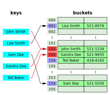
## Ссылки
- [Wikipedia](https://ru.wikipedia.org/wiki/%D0%A5%D0%B5%D1%88-%D1%82%D0%B0%D0%B1%D0%BB%D0%B8%D1%86%D0%B0)
- [YouTube](https://www.youtube.com/watch?v=rVr1y32fDI0)
================================================
FILE: src/data-structures/hash-table/README.uk-UA.md
================================================
# Геш таблиця
**Геш таблиця** - структура даних, що реалізує абстрактний тип даних асоціативний масив, тобто. структура, яка
_зв'язує ключі зі значеннями_. Геш-таблиця використовує _геш-функцію_ для обчислення індексу в масиві, в якому може
бути знайдено бажане значення. Нижче представлена геш-таблиця, у якій ключем виступає ім'я людини, а значеннями
телефонні номери. Геш-функція перетворює ключ-ім'я на індекс масиву з телефонними номерами.

В ідеалі геш-функція присвоюватиме елементу масиву унікальний ключ. Проте більшість реальних геш-таблиць
використовують недосконалі геш-функції. Це може призвести до ситуацій, коли геш-функція генерує однаковий індекс для
кількох ключів. Ці ситуації називаються колізіями і мають бути якось вирішені.
Існує два варіанти вирішення колізій - геш-таблиця з ланцюжками та з відкритою адресацією.
Метод ланцюжків передбачає зберігання значень, відповідних одному й тому індексу як зв'язкового списку(ланцюжка).

_Made with [okso.app](https://okso.app)_
Метод відкритої адресації поміщає значення, для якого отримано дублюючий індекс, в першу вільну комірку.

## Посилання
- [Wikipedia](https://uk.wikipedia.org/wiki/%D0%93%D0%B5%D1%88-%D1%82%D0%B0%D0%B1%D0%BB%D0%B8%D1%86%D1%8F)
- [YouTube](https://www.youtube.com/watch?v=WTYaboK-NMk)
================================================
FILE: src/data-structures/hash-table/README.zh-CN.md
================================================
# 哈希表
在计算中, 一个 **哈希表(hash table 或hash map)** 是一种实现 *关联数组(associative array)*
的抽象数据类型, 该结构可以将 *键映射到值*。
哈希表使用 *哈希函数/散列函数* 来计算一个值在数组或桶(buckets)中或槽(slots)中对应的索引,可使用该索引找到所需的值。
理想情况下,散列函数将为每个键分配给一个唯一的桶(bucket),但是大多数哈希表设计采用不完美的散列函数,这可能会导致"哈希冲突(hash collisions)",也就是散列函数为多个键(key)生成了相同的索引,这种碰撞必须
以某种方式进行处理。

*Made with [okso.app](https://okso.app)*
通过单独的链接解决哈希冲突

*Made with [okso.app](https://okso.app)*
## 参考
- [Wikipedia](https://en.wikipedia.org/wiki/Hash_table)
- [YouTube](https://www.youtube.com/watch?v=shs0KM3wKv8&index=4&list=PLLXdhg_r2hKA7DPDsunoDZ-Z769jWn4R8)
================================================
FILE: src/data-structures/hash-table/__test__/HashTable.test.js
================================================
import HashTable from '../HashTable';
describe('HashTable', () => {
it('should create hash table of certain size', () => {
const defaultHashTable = new HashTable();
expect(defaultHashTable.buckets.length).toBe(32);
const biggerHashTable = new HashTable(64);
expect(biggerHashTable.buckets.length).toBe(64);
});
it('should generate proper hash for specified keys', () => {
const hashTable = new HashTable();
expect(hashTable.hash('a')).toBe(1);
expect(hashTable.hash('b')).toBe(2);
expect(hashTable.hash('abc')).toBe(6);
});
it('should set, read and delete data with collisions', () => {
const hashTable = new HashTable(3);
expect(hashTable.hash('a')).toBe(1);
expect(hashTable.hash('b')).toBe(2);
expect(hashTable.hash('c')).toBe(0);
expect(hashTable.hash('d')).toBe(1);
hashTable.set('a', 'sky-old');
hashTable.set('a', 'sky');
hashTable.set('b', 'sea');
hashTable.set('c', 'earth');
hashTable.set('d', 'ocean');
expect(hashTable.has('x')).toBe(false);
expect(hashTable.has('b')).toBe(true);
expect(hashTable.has('c')).toBe(true);
const stringifier = (value) => `${value.key}:${value.value}`;
expect(hashTable.buckets[0].toString(stringifier)).toBe('c:earth');
expect(hashTable.buckets[1].toString(stringifier)).toBe('a:sky,d:ocean');
expect(hashTable.buckets[2].toString(stringifier)).toBe('b:sea');
expect(hashTable.get('a')).toBe('sky');
expect(hashTable.get('d')).toBe('ocean');
expect(hashTable.get('x')).not.toBeDefined();
hashTable.delete('a');
expect(hashTable.delete('not-existing')).toBeNull();
expect(hashTable.get('a')).not.toBeDefined();
expect(hashTable.get('d')).toBe('ocean');
hashTable.set('d', 'ocean-new');
expect(hashTable.get('d')).toBe('ocean-new');
});
it('should be possible to add objects to hash table', () => {
const hashTable = new HashTable();
hashTable.set('objectKey', { prop1: 'a', prop2: 'b' });
const object = hashTable.get('objectKey');
expect(object).toBeDefined();
expect(object.prop1).toBe('a');
expect(object.prop2).toBe('b');
});
it('should track actual keys', () => {
const hashTable = new HashTable(3);
hashTable.set('a', 'sky-old');
hashTable.set('a', 'sky');
hashTable.set('b', 'sea');
hashTable.set('c', 'earth');
hashTable.set('d', 'ocean');
expect(hashTable.getKeys()).toEqual(['a', 'b', 'c', 'd']);
expect(hashTable.has('a')).toBe(true);
expect(hashTable.has('x')).toBe(false);
hashTable.delete('a');
expect(hashTable.has('a')).toBe(false);
expect(hashTable.has('b')).toBe(true);
expect(hashTable.has('x')).toBe(false);
});
it('should get all the values', () => {
const hashTable = new HashTable(3);
hashTable.set('a', 'alpha');
hashTable.set('b', 'beta');
hashTable.set('c', 'gamma');
expect(hashTable.getValues()).toEqual(['gamma', 'alpha', 'beta']);
});
it('should get all the values from empty hash table', () => {
const hashTable = new HashTable();
expect(hashTable.getValues()).toEqual([]);
});
it('should get all the values in case of hash collision', () => {
const hashTable = new HashTable(3);
// Keys `ab` and `ba` in current implementation should result in one hash (one bucket).
// We need to make sure that several items from one bucket will be serialized.
hashTable.set('ab', 'one');
hashTable.set('ba', 'two');
hashTable.set('ac', 'three');
expect(hashTable.getValues()).toEqual(['one', 'two', 'three']);
});
});
================================================
FILE: src/data-structures/heap/Heap.js
================================================
import Comparator from '../../utils/comparator/Comparator';
/**
* Parent class for Min and Max Heaps.
*/
export default class Heap {
/**
* @constructs Heap
* @param {Function} [comparatorFunction]
*/
constructor(comparatorFunction) {
if (new.target === Heap) {
throw new TypeError('Cannot construct Heap instance directly');
}
// Array representation of the heap.
this.heapContainer = [];
this.compare = new Comparator(comparatorFunction);
}
/**
* @param {number} parentIndex
* @return {number}
*/
getLeftChildIndex(parentIndex) {
return (2 * parentIndex) + 1;
}
/**
* @param {number} parentIndex
* @return {number}
*/
getRightChildIndex(parentIndex) {
return (2 * parentIndex) + 2;
}
/**
* @param {number} childIndex
* @return {number}
*/
getParentIndex(childIndex) {
return Math.floor((childIndex - 1) / 2);
}
/**
* @param {number} childIndex
* @return {boolean}
*/
hasParent(childIndex) {
return this.getParentIndex(childIndex) >= 0;
}
/**
* @param {number} parentIndex
* @return {boolean}
*/
hasLeftChild(parentIndex) {
return this.getLeftChildIndex(parentIndex) < this.heapContainer.length;
}
/**
* @param {number} parentIndex
* @return {boolean}
*/
hasRightChild(parentIndex) {
return this.getRightChildIndex(parentIndex) < this.heapContainer.length;
}
/**
* @param {number} parentIndex
* @return {*}
*/
leftChild(parentIndex) {
return this.heapContainer[this.getLeftChildIndex(parentIndex)];
}
/**
* @param {number} parentIndex
* @return {*}
*/
rightChild(parentIndex) {
return this.heapContainer[this.getRightChildIndex(parentIndex)];
}
/**
* @param {number} childIndex
* @return {*}
*/
parent(childIndex) {
return this.heapContainer[this.getParentIndex(childIndex)];
}
/**
* @param {number} indexOne
* @param {number} indexTwo
*/
swap(indexOne, indexTwo) {
const tmp = this.heapContainer[indexTwo];
this.heapContainer[indexTwo] = this.heapContainer[indexOne];
this.heapContainer[indexOne] = tmp;
}
/**
* @return {*}
*/
peek() {
if (this.heapContainer.length === 0) {
return null;
}
return this.heapContainer[0];
}
/**
* @return {*}
*/
poll() {
if (this.heapContainer.length === 0) {
return null;
}
if (this.heapContainer.length === 1) {
return this.heapContainer.pop();
}
const item = this.heapContainer[0];
// Move the last element from the end to the head.
this.heapContainer[0] = this.heapContainer.pop();
this.heapifyDown();
return item;
}
/**
* @param {*} item
* @return {Heap}
*/
add(item) {
this.heapContainer.push(item);
this.heapifyUp();
return this;
}
/**
* @param {*} item
* @param {Comparator} [comparator]
* @return {Heap}
*/
remove(item, comparator = this.compare) {
// Find number of items to remove.
const numberOfItemsToRemove = this.find(item, comparator).length;
for (let iteration = 0; iteration < numberOfItemsToRemove; iteration += 1) {
// We need to find item index to remove each time after removal since
// indices are being changed after each heapify process.
const indexToRemove = this.find(item, comparator).pop();
// If we need to remove last child in the heap then just remove it.
// There is no need to heapify the heap afterwards.
if (indexToRemove === (this.heapContainer.length - 1)) {
this.heapContainer.pop();
} else {
// Move last element in heap to the vacant (removed) position.
this.heapContainer[indexToRemove] = this.heapContainer.pop();
// Get parent.
const parentItem = this.parent(indexToRemove);
// If there is no parent or parent is in correct order with the node
// we're going to delete then heapify down. Otherwise heapify up.
if (
this.hasLeftChild(indexToRemove)
&& (
!parentItem
|| this.pairIsInCorrectOrder(parentItem, this.heapContainer[indexToRemove])
)
) {
this.heapifyDown(indexToRemove);
} else {
this.heapifyUp(indexToRemove);
}
}
}
return this;
}
/**
* @param {*} item
* @param {Comparator} [comparator]
* @return {Number[]}
*/
find(item, comparator = this.compare) {
const foundItemIndices = [];
for (let itemIndex = 0; itemIndex < this.heapContainer.length; itemIndex += 1) {
if (comparator.equal(item, this.heapContainer[itemIndex])) {
foundItemIndices.push(itemIndex);
}
}
return foundItemIndices;
}
/**
* @return {boolean}
*/
isEmpty() {
return !this.heapContainer.length;
}
/**
* @return {string}
*/
toString() {
return this.heapContainer.toString();
}
/**
* @param {number} [customStartIndex]
*/
heapifyUp(customStartIndex) {
// Take the last element (last in array or the bottom left in a tree)
// in the heap container and lift it up until it is in the correct
// order with respect to its parent element.
let currentIndex = customStartIndex || this.heapContainer.length - 1;
while (
this.hasParent(currentIndex)
&& !this.pairIsInCorrectOrder(this.parent(currentIndex), this.heapContainer[currentIndex])
) {
this.swap(currentIndex, this.getParentIndex(currentIndex));
currentIndex = this.getParentIndex(currentIndex);
}
}
/**
* @param {number} [customStartIndex]
*/
heapifyDown(customStartIndex = 0) {
// Compare the parent element to its children and swap parent with the appropriate
// child (smallest child for MinHeap, largest child for MaxHeap).
// Do the same for next children after swap.
let currentIndex = customStartIndex;
let nextIndex = null;
while (this.hasLeftChild(currentIndex)) {
if (
this.hasRightChild(currentIndex)
&& this.pairIsInCorrectOrder(this.rightChild(currentIndex), this.leftChild(currentIndex))
) {
nextIndex = this.getRightChildIndex(currentIndex);
} else {
nextIndex = this.getLeftChildIndex(currentIndex);
}
if (this.pairIsInCorrectOrder(
this.heapContainer[currentIndex],
this.heapContainer[nextIndex],
)) {
break;
}
this.swap(currentIndex, nextIndex);
currentIndex = nextIndex;
}
}
/**
* Checks if pair of heap elements is in correct order.
* For MinHeap the first element must be always smaller or equal.
* For MaxHeap the first element must be always bigger or equal.
*
* @param {*} firstElement
* @param {*} secondElement
* @return {boolean}
*/
/* istanbul ignore next */
pairIsInCorrectOrder(firstElement, secondElement) {
throw new Error(`
You have to implement heap pair comparison method
for ${firstElement} and ${secondElement} values.
`);
}
}
================================================
FILE: src/data-structures/heap/MaxHeap.js
================================================
import Heap from './Heap';
export default class MaxHeap extends Heap {
/**
* Checks if pair of heap elements is in correct order.
* For MinHeap the first element must be always smaller or equal.
* For MaxHeap the first element must be always bigger or equal.
*
* @param {*} firstElement
* @param {*} secondElement
* @return {boolean}
*/
pairIsInCorrectOrder(firstElement, secondElement) {
return this.compare.greaterThanOrEqual(firstElement, secondElement);
}
}
================================================
FILE: src/data-structures/heap/MaxHeapAdhoc.js
================================================
/**
* The minimalistic (ad hoc) version of a MaxHeap data structure that doesn't have
* external dependencies and that is easy to copy-paste and use during the
* coding interview if allowed by the interviewer (since many data
* structures in JS are missing).
*/
class MaxHeapAdhoc {
constructor(heap = []) {
this.heap = [];
heap.forEach(this.add);
}
add(num) {
this.heap.push(num);
this.heapifyUp();
}
peek() {
return this.heap[0];
}
poll() {
if (this.heap.length === 0) return undefined;
const top = this.heap[0];
this.heap[0] = this.heap[this.heap.length - 1];
this.heap.pop();
this.heapifyDown();
return top;
}
isEmpty() {
return this.heap.length === 0;
}
toString() {
return this.heap.join(',');
}
heapifyUp() {
let nodeIndex = this.heap.length - 1;
while (nodeIndex > 0) {
const parentIndex = this.getParentIndex(nodeIndex);
if (this.heap[parentIndex] >= this.heap[nodeIndex]) break;
this.swap(parentIndex, nodeIndex);
nodeIndex = parentIndex;
}
}
heapifyDown() {
let nodeIndex = 0;
while (
(
this.hasLeftChild(nodeIndex) && this.heap[nodeIndex] < this.leftChild(nodeIndex)
)
|| (
this.hasRightChild(nodeIndex) && this.heap[nodeIndex] < this.rightChild(nodeIndex)
)
) {
const leftIndex = this.getLeftChildIndex(nodeIndex);
const rightIndex = this.getRightChildIndex(nodeIndex);
const left = this.leftChild(nodeIndex);
const right = this.rightChild(nodeIndex);
if (this.hasLeftChild(nodeIndex) && this.hasRightChild(nodeIndex)) {
if (left >= right) {
this.swap(leftIndex, nodeIndex);
nodeIndex = leftIndex;
} else {
this.swap(rightIndex, nodeIndex);
nodeIndex = rightIndex;
}
} else if (this.hasLeftChild(nodeIndex)) {
this.swap(leftIndex, nodeIndex);
nodeIndex = leftIndex;
}
}
}
getLeftChildIndex(parentIndex) {
return (2 * parentIndex) + 1;
}
getRightChildIndex(parentIndex) {
return (2 * parentIndex) + 2;
}
getParentIndex(childIndex) {
return Math.floor((childIndex - 1) / 2);
}
hasLeftChild(parentIndex) {
return this.getLeftChildIndex(parentIndex) < this.heap.length;
}
hasRightChild(parentIndex) {
return this.getRightChildIndex(parentIndex) < this.heap.length;
}
leftChild(parentIndex) {
return this.heap[this.getLeftChildIndex(parentIndex)];
}
rightChild(parentIndex) {
return this.heap[this.getRightChildIndex(parentIndex)];
}
swap(indexOne, indexTwo) {
const tmp = this.heap[indexTwo];
this.heap[indexTwo] = this.heap[indexOne];
this.heap[indexOne] = tmp;
}
}
export default MaxHeapAdhoc;
================================================
FILE: src/data-structures/heap/MinHeap.js
================================================
import Heap from './Heap';
export default class MinHeap extends Heap {
/**
* Checks if pair of heap elements is in correct order.
* For MinHeap the first element must be always smaller or equal.
* For MaxHeap the first element must be always bigger or equal.
*
* @param {*} firstElement
* @param {*} secondElement
* @return {boolean}
*/
pairIsInCorrectOrder(firstElement, secondElement) {
return this.compare.lessThanOrEqual(firstElement, secondElement);
}
}
================================================
FILE: src/data-structures/heap/MinHeapAdhoc.js
================================================
/**
* The minimalistic (ad hoc) version of a MinHeap data structure that doesn't have
* external dependencies and that is easy to copy-paste and use during the
* coding interview if allowed by the interviewer (since many data
* structures in JS are missing).
*/
class MinHeapAdhoc {
constructor(heap = []) {
this.heap = [];
heap.forEach(this.add);
}
add(num) {
this.heap.push(num);
this.heapifyUp();
}
peek() {
return this.heap[0];
}
poll() {
if (this.heap.length === 0) return undefined;
const top = this.heap[0];
this.heap[0] = this.heap[this.heap.length - 1];
this.heap.pop();
this.heapifyDown();
return top;
}
isEmpty() {
return this.heap.length === 0;
}
toString() {
return this.heap.join(',');
}
heapifyUp() {
let nodeIndex = this.heap.length - 1;
while (nodeIndex > 0) {
const parentIndex = this.getParentIndex(nodeIndex);
if (this.heap[parentIndex] <= this.heap[nodeIndex]) break;
this.swap(parentIndex, nodeIndex);
nodeIndex = parentIndex;
}
}
heapifyDown() {
let nodeIndex = 0;
while (
(
this.hasLeftChild(nodeIndex)
&& this.heap[nodeIndex] > this.leftChild(nodeIndex)
)
|| (
this.hasRightChild(nodeIndex)
&& this.heap[nodeIndex] > this.rightChild(nodeIndex)
)
) {
const leftIndex = this.getLeftChildIndex(nodeIndex);
const rightIndex = this.getRightChildIndex(nodeIndex);
const left = this.leftChild(nodeIndex);
const right = this.rightChild(nodeIndex);
if (this.hasLeftChild(nodeIndex) && this.hasRightChild(nodeIndex)) {
if (left <= right) {
this.swap(leftIndex, nodeIndex);
nodeIndex = leftIndex;
} else {
this.swap(rightIndex, nodeIndex);
nodeIndex = rightIndex;
}
} else if (this.hasLeftChild(nodeIndex)) {
this.swap(leftIndex, nodeIndex);
nodeIndex = leftIndex;
}
}
}
getLeftChildIndex(parentIndex) {
return 2 * parentIndex + 1;
}
getRightChildIndex(parentIndex) {
return 2 * parentIndex + 2;
}
getParentIndex(childIndex) {
return Math.floor((childIndex - 1) / 2);
}
hasLeftChild(parentIndex) {
return this.getLeftChildIndex(parentIndex) < this.heap.length;
}
hasRightChild(parentIndex) {
return this.getRightChildIndex(parentIndex) < this.heap.length;
}
leftChild(parentIndex) {
return this.heap[this.getLeftChildIndex(parentIndex)];
}
rightChild(parentIndex) {
return this.heap[this.getRightChildIndex(parentIndex)];
}
swap(indexOne, indexTwo) {
const tmp = this.heap[indexTwo];
this.heap[indexTwo] = this.heap[indexOne];
this.heap[indexOne] = tmp;
}
}
export default MinHeapAdhoc;
================================================
FILE: src/data-structures/heap/README.fr-FR.md
================================================
# Tas (structure de données)
En informatique, un **tas** est une structure de données arborescente spécialisée qui satisfait la propriété de tas décrite ci-dessous.
Dans un *tas minimal* (en anglais *min heap*), si `P` est un nœud parent de `C`, alors la clé (la valeur) de `P` est inférieure ou égale à la clé de `C`.

*Made with [okso.app](https://okso.app)*
Dans un *tas maximal* (en anglais *max heap*), la clé de `P` est supérieure ou égale à la clé de `C`.


Le nœud au «sommet» du tas sans parents est appelé le nœud racine.
## Références
- [Wikipedia](https://fr.wikipedia.org/wiki/Tas_(informatique))
- [YouTube](https://www.youtube.com/watch?v=t0Cq6tVNRBA&index=5&t=0s&list=PLLXdhg_r2hKA7DPDsunoDZ-Z769jWn4R8)
================================================
FILE: src/data-structures/heap/README.ja-JP.md
================================================
# ヒープ (データ構造)
コンピュータサイエンスにおいて、*ヒープ*は特殊な木構造のデータ構造で、後述するヒープの特性を持っています。
*最小ヒープ*では、もし`P`が`C`の親ノードの場合、`P`のキー(値)は`C`のキーより小さい、または等しくなります。

*Made with [okso.app](https://okso.app)*
*最大ヒープ*では、`P`のキーは`C`のキーより大きい、もしくは等しくなります。


ヒープの「トップ」のノードには親ノードが存在せず、ルートノードと呼ばれます。
## 参考
- [Wikipedia](https://en.wikipedia.org/wiki/Heap_(data_structure))
- [YouTube](https://www.youtube.com/watch?v=t0Cq6tVNRBA&index=5&t=0s&list=PLLXdhg_r2hKA7DPDsunoDZ-Z769jWn4R8)
================================================
FILE: src/data-structures/heap/README.ko-KR.md
================================================
# 힙 (자료구조)
컴퓨터 과학에서의 **힙**은 아래에 설명된 힙 속성을 만족하는 전문화된 트리 기반 데이터구조입니다.
*최소 힙*에서 `P`가 `C`의 상위 노드라면 `P`의 키(값)는 `C`의 키보다 작거나 같습니다.

*Made with [okso.app](https://okso.app)*
*최대 힙*에서 `P`의 키는 `C`의 키보다 크거나 같습니다.


상위 노드가 없는 힙의 "상단"에 있는 노드를 루트 노드라고 합니다.
## 참조
- [Wikipedia]()
- [YouTube](https://www.youtube.com/watch?v=t0Cq6tVNRBA&index=5&t=0s&list=PLLXdhg_r2hKA7DPDsunoDZ-Z769jWn4R8)
================================================
FILE: src/data-structures/heap/README.md
================================================
# Heap (data-structure)
_Read this in other languages:_
[_简体中文_](README.zh-CN.md),
[_Русский_](README.ru-RU.md),
[_日本語_](README.ja-JP.md),
[_Français_](README.fr-FR.md),
[_Português_](README.pt-BR.md),
[_Türkçe_](README.tr-TR.md),
[_한국어_](README.ko-KR.md),
[_Українська_](README.uk-UA.md)
In computer science, a **heap** is a specialized tree-based
data structure that satisfies the heap property described
below.
In a *min heap*, if `P` is a parent node of `C`, then the
key (the value) of `P` is less than or equal to the
key of `C`.

*Made with [okso.app](https://okso.app)*
In a *max heap*, the key of `P` is greater than or equal
to the key of `C`


The node at the "top" of the heap with no parents is
called the root node.
## Time Complexities
Here are time complexities of various heap data structures. Function names assume a max-heap.
| Operation | find-max | delete-max | insert| increase-key| meld |
| --------- | -------- | ---------- | ----- | ----------- | ---- |
| [Binary](https://en.wikipedia.org/wiki/Binary_heap) | `Θ(1)` | `Θ(log n)` | `O(log n)` | `O(log n)` | `Θ(n)` |
| [Leftist](https://en.wikipedia.org/wiki/Leftist_tree) | `Θ(1)` | `Θ(log n)` | `Θ(log n)` | `O(log n)` | `Θ(log n)` |
| [Binomial](https://en.wikipedia.org/wiki/Binomial_heap) | `Θ(1)` | `Θ(log n)` | `Θ(1)` | `O(log n)` | `O(log n)` |
| [Fibonacci](https://en.wikipedia.org/wiki/Fibonacci_heap) | `Θ(1)` | `Θ(log n)` | `Θ(1)` | `Θ(1)` | `Θ(1)` |
| [Pairing](https://en.wikipedia.org/wiki/Pairing_heap) | `Θ(1)` | `Θ(log n)` | `Θ(1)` | `o(log n)` | `Θ(1)` |
| [Brodal](https://en.wikipedia.org/wiki/Brodal_queue) | `Θ(1)` | `Θ(log n)` | `Θ(1)` | `Θ(1)` | `Θ(1)` |
| [Rank-pairing](https://en.wikipedia.org/w/index.php?title=Rank-pairing_heap&action=edit&redlink=1) | `Θ(1)` | `Θ(log n)` | `Θ(1)` | `Θ(1)` | `Θ(1)` |
| [Strict Fibonacci](https://en.wikipedia.org/wiki/Fibonacci_heap) | `Θ(1)` | `Θ(log n)` | `Θ(1)` | `Θ(1)` | `Θ(1)` |
| [2-3 heap](https://en.wikipedia.org/wiki/2%E2%80%933_heap) | `O(log n)` | `O(log n)` | `O(log n)` | `Θ(1)` | `?` |
Where:
- **find-max (or find-min):** find a maximum item of a max-heap, or a minimum item of a min-heap, respectively (a.k.a. *peek*)
- **delete-max (or delete-min):** removing the root node of a max heap (or min heap), respectively
- **insert:** adding a new key to the heap (a.k.a., *push*)
- **increase-key or decrease-key:** updating a key within a max- or min-heap, respectively
- **meld:** joining two heaps to form a valid new heap containing all the elements of both, destroying the original heaps.
> In this repository, the [MaxHeap.js](./MaxHeap.js) and [MinHeap.js](./MinHeap.js) are examples of the **Binary** heap.
## Implementation
- [MaxHeap.js](./MaxHeap.js) and [MinHeap.js](./MinHeap.js)
- [MaxHeapAdhoc.js](./MaxHeapAdhoc.js) and [MinHeapAdhoc.js](./MinHeapAdhoc.js) - The minimalistic (ad hoc) version of a MinHeap/MaxHeap data structure that doesn't have external dependencies and that is easy to copy-paste and use during the coding interview if allowed by the interviewer (since many data structures in JS are missing).
## References
- [Wikipedia](https://en.wikipedia.org/wiki/Heap_(data_structure))
- [YouTube](https://www.youtube.com/watch?v=t0Cq6tVNRBA&index=5&t=0s&list=PLLXdhg_r2hKA7DPDsunoDZ-Z769jWn4R8)
================================================
FILE: src/data-structures/heap/README.pt-BR.md
================================================
# Heap (estrutura de dados)
Na ciência da computação, um **heap** é uma estrutura de dados
baseada em uma árvore especializada que satisfaz a propriedade _heap_ descrita abaixo.
Em um *heap mínimo* (min heap), caso `P` é um nó pai de `C`, então a chave
(o valor) de `P` é menor ou igual a chave de `C`.

*Made with [okso.app](https://okso.app)*
Em uma *heap máximo* (max heap), a chave de `P` é maior ou igual
a chave de `C`.


O nó no "topo" do _heap_, cujo não possui pais, é chamado de nó raiz.
## References
- [Wikipedia](https://en.wikipedia.org/wiki/Heap_(data_structure))
- [YouTube](https://www.youtube.com/watch?v=t0Cq6tVNRBA&index=5&t=0s&list=PLLXdhg_r2hKA7DPDsunoDZ-Z769jWn4R8)
================================================
FILE: src/data-structures/heap/README.ru-RU.md
================================================
# Куча (структура данных)
В компьютерных науках куча — это специализированная структура данных типа дерево, которая удовлетворяет свойству кучи:
если B является узлом-потомком узла A, то ключ(A) ≥ ключ(B). Из этого следует, что элемент с наибольшим ключом всегда
является корневым узлом кучи, поэтому иногда такие кучи называют max-кучами.


Если сравнение перевернуть, то наименьший элемент будет всегда корневым узлом, такие кучи называют min-кучами.

*Made with [okso.app](https://okso.app)*
Не существует никаких ограничений относительно того, сколько узлов-потомков имеет каждый узел кучи. На практике их
число обычно не более двух. Куча является максимально эффективной реализацией абстрактного типа данных, который
называется очередью с приоритетом.
Узел на вершине кучи, у которого нет родителей, называется корневым узлом.
## Ссылки
- [Wikipedia](https://ru.wikipedia.org/wiki/Куча_(структура_данных))
- [YouTube](https://www.youtube.com/watch?v=noQ4SUoqrQA)
================================================
FILE: src/data-structures/heap/README.tr-TR.md
================================================
# Heap (data-structure)
Bilgisayar biliminde, **yığın (heap)** aşağıda açıklanan özellikleri karşılayan ağaç tabanlı(tree-based) özel bir veri yapısıdır.
*min heap*, Eğer `P`, `C`'nin üst düğümü ise, `P`'nin anahtarı (değeri) `C`'nin anahtarından (değerinden) küçük veya ona eşittir.

*Made with [okso.app](https://okso.app)*
*max heap*, `P`'nin anahtarı `C`'nin anahtarından büyük veya eşittir.


Yığının (Heap) "en üstündeki" ebeveyni olmayan düğüme kök düğüm (root node) denir.
## Referanslar
- [Wikipedia](https://en.wikipedia.org/wiki/Heap_(data_structure))
- [YouTube](https://www.youtube.com/watch?v=t0Cq6tVNRBA&index=5&t=0s&list=PLLXdhg_r2hKA7DPDsunoDZ-Z769jWn4R8)
================================================
FILE: src/data-structures/heap/README.uk-UA.md
================================================
# Купа (структура даних)
У комп'ютерних науках купа - це спеціалізована структура даних на кшталт дерева, яка задовольняє властивості купи:
якщо B є вузлом-нащадком вузла A, то ключ (A) ≥ ключ (B). З цього випливає, що елемент із найбільшим ключем завжди
є кореневим вузлом купи, тому іноді такі купи називають max-купами.


Якщо порівняння перевернути, то найменший елемент завжди буде кореневим вузлом, такі купи називають min-купами.

*Made with [okso.app](https://okso.app)*
Не існує жодних обмежень щодо того, скільки вузлів-нащадків має кожен вузол купи. На практиці їх
число зазвичай трохи більше двох. Купа є максимально ефективною реалізацією абстрактного типу даних, який
називається чергою із пріоритетом.
Вузол на вершині купи, який не має батьків, називається кореневим вузлом.
## Посилання
- [Wikipedia](https://uk.wikipedia.org/wiki/%D0%9A%D1%83%D0%BF%D0%B0_(%D1%81%D1%82%D1%80%D1%83%D0%BA%D1%82%D1%83%D1%80%D0%B0_%D0%B4%D0%B0%D0%BD%D0%B8%D1%85))
================================================
FILE: src/data-structures/heap/README.zh-CN.md
================================================
# 堆 (数据结构)
在计算机科学中, 一个 **堆(heap)** 是一种特殊的基于树的数据结构,它满足下面描述的堆属性。
在一个 *最小堆(min heap)* 中, 如果 `P` 是 `C` 的一个父级节点, 那么 `P` 的key(或value)应小于或等于 `C` 的对应值.

*Made with [okso.app](https://okso.app)*
在一个 *最大堆(max heap)* 中, `P` 的key(或value)大于 `C` 的对应值。


在堆“顶部”的没有父级节点的节点,被称之为根节点。
## 参考
- [Wikipedia](https://en.wikipedia.org/wiki/Heap_(data_structure))
- [YouTube](https://www.youtube.com/watch?v=t0Cq6tVNRBA&index=5&t=0s&list=PLLXdhg_r2hKA7DPDsunoDZ-Z769jWn4R8)
================================================
FILE: src/data-structures/heap/__test__/Heap.test.js
================================================
import Heap from '../Heap';
describe('Heap', () => {
it('should not allow to create instance of the Heap directly', () => {
const instantiateHeap = () => {
const heap = new Heap();
heap.add(5);
};
expect(instantiateHeap).toThrow();
});
});
================================================
FILE: src/data-structures/heap/__test__/MaxHeap.test.js
================================================
import MaxHeap from '../MaxHeap';
import Comparator from '../../../utils/comparator/Comparator';
describe('MaxHeap', () => {
it('should create an empty max heap', () => {
const maxHeap = new MaxHeap();
expect(maxHeap).toBeDefined();
expect(maxHeap.peek()).toBeNull();
expect(maxHeap.isEmpty()).toBe(true);
});
it('should add items to the heap and heapify it up', () => {
const maxHeap = new MaxHeap();
maxHeap.add(5);
expect(maxHeap.isEmpty()).toBe(false);
expect(maxHeap.peek()).toBe(5);
expect(maxHeap.toString()).toBe('5');
maxHeap.add(3);
expect(maxHeap.peek()).toBe(5);
expect(maxHeap.toString()).toBe('5,3');
maxHeap.add(10);
expect(maxHeap.peek()).toBe(10);
expect(maxHeap.toString()).toBe('10,3,5');
maxHeap.add(1);
expect(maxHeap.peek()).toBe(10);
expect(maxHeap.toString()).toBe('10,3,5,1');
maxHeap.add(1);
expect(maxHeap.peek()).toBe(10);
expect(maxHeap.toString()).toBe('10,3,5,1,1');
expect(maxHeap.poll()).toBe(10);
expect(maxHeap.toString()).toBe('5,3,1,1');
expect(maxHeap.poll()).toBe(5);
expect(maxHeap.toString()).toBe('3,1,1');
expect(maxHeap.poll()).toBe(3);
expect(maxHeap.toString()).toBe('1,1');
});
it('should poll items from the heap and heapify it down', () => {
const maxHeap = new MaxHeap();
maxHeap.add(5);
maxHeap.add(3);
maxHeap.add(10);
maxHeap.add(11);
maxHeap.add(1);
expect(maxHeap.toString()).toBe('11,10,5,3,1');
expect(maxHeap.poll()).toBe(11);
expect(maxHeap.toString()).toBe('10,3,5,1');
expect(maxHeap.poll()).toBe(10);
expect(maxHeap.toString()).toBe('5,3,1');
expect(maxHeap.poll()).toBe(5);
expect(maxHeap.toString()).toBe('3,1');
expect(maxHeap.poll()).toBe(3);
expect(maxHeap.toString()).toBe('1');
expect(maxHeap.poll()).toBe(1);
expect(maxHeap.toString()).toBe('');
expect(maxHeap.poll()).toBeNull();
expect(maxHeap.toString()).toBe('');
});
it('should heapify down through the right branch as well', () => {
const maxHeap = new MaxHeap();
maxHeap.add(3);
maxHeap.add(12);
maxHeap.add(10);
expect(maxHeap.toString()).toBe('12,3,10');
maxHeap.add(11);
expect(maxHeap.toString()).toBe('12,11,10,3');
expect(maxHeap.poll()).toBe(12);
expect(maxHeap.toString()).toBe('11,3,10');
});
it('should be possible to find item indices in heap', () => {
const maxHeap = new MaxHeap();
maxHeap.add(3);
maxHeap.add(12);
maxHeap.add(10);
maxHeap.add(11);
maxHeap.add(11);
expect(maxHeap.toString()).toBe('12,11,10,3,11');
expect(maxHeap.find(5)).toEqual([]);
expect(maxHeap.find(12)).toEqual([0]);
expect(maxHeap.find(11)).toEqual([1, 4]);
});
it('should be possible to remove items from heap with heapify down', () => {
const maxHeap = new MaxHeap();
maxHeap.add(3);
maxHeap.add(12);
maxHeap.add(10);
maxHeap.add(11);
maxHeap.add(11);
expect(maxHeap.toString()).toBe('12,11,10,3,11');
expect(maxHeap.remove(12).toString()).toEqual('11,11,10,3');
expect(maxHeap.remove(12).peek()).toEqual(11);
expect(maxHeap.remove(11).toString()).toEqual('10,3');
expect(maxHeap.remove(10).peek()).toEqual(3);
});
it('should be possible to remove items from heap with heapify up', () => {
const maxHeap = new MaxHeap();
maxHeap.add(3);
maxHeap.add(10);
maxHeap.add(5);
maxHeap.add(6);
maxHeap.add(7);
maxHeap.add(4);
maxHeap.add(6);
maxHeap.add(8);
maxHeap.add(2);
maxHeap.add(1);
expect(maxHeap.toString()).toBe('10,8,6,7,6,4,5,3,2,1');
expect(maxHeap.remove(4).toString()).toEqual('10,8,6,7,6,1,5,3,2');
expect(maxHeap.remove(3).toString()).toEqual('10,8,6,7,6,1,5,2');
expect(maxHeap.remove(5).toString()).toEqual('10,8,6,7,6,1,2');
expect(maxHeap.remove(10).toString()).toEqual('8,7,6,2,6,1');
expect(maxHeap.remove(6).toString()).toEqual('8,7,1,2');
expect(maxHeap.remove(2).toString()).toEqual('8,7,1');
expect(maxHeap.remove(1).toString()).toEqual('8,7');
expect(maxHeap.remove(7).toString()).toEqual('8');
expect(maxHeap.remove(8).toString()).toEqual('');
});
it('should be possible to remove items from heap with custom finding comparator', () => {
const maxHeap = new MaxHeap();
maxHeap.add('a');
maxHeap.add('bb');
maxHeap.add('ccc');
maxHeap.add('dddd');
expect(maxHeap.toString()).toBe('dddd,ccc,bb,a');
const comparator = new Comparator((a, b) => {
if (a.length === b.length) {
return 0;
}
return a.length < b.length ? -1 : 1;
});
maxHeap.remove('hey', comparator);
expect(maxHeap.toString()).toBe('dddd,a,bb');
});
});
================================================
FILE: src/data-structures/heap/__test__/MaxHeapAdhoc.test.js
================================================
import MaxHeap from '../MaxHeapAdhoc';
describe('MaxHeapAdhoc', () => {
it('should create an empty max heap', () => {
const maxHeap = new MaxHeap();
expect(maxHeap).toBeDefined();
expect(maxHeap.peek()).toBe(undefined);
expect(maxHeap.isEmpty()).toBe(true);
});
it('should add items to the heap and heapify it up', () => {
const maxHeap = new MaxHeap();
maxHeap.add(5);
expect(maxHeap.isEmpty()).toBe(false);
expect(maxHeap.peek()).toBe(5);
expect(maxHeap.toString()).toBe('5');
maxHeap.add(3);
expect(maxHeap.peek()).toBe(5);
expect(maxHeap.toString()).toBe('5,3');
maxHeap.add(10);
expect(maxHeap.peek()).toBe(10);
expect(maxHeap.toString()).toBe('10,3,5');
maxHeap.add(1);
expect(maxHeap.peek()).toBe(10);
expect(maxHeap.toString()).toBe('10,3,5,1');
maxHeap.add(1);
expect(maxHeap.peek()).toBe(10);
expect(maxHeap.toString()).toBe('10,3,5,1,1');
expect(maxHeap.poll()).toBe(10);
expect(maxHeap.toString()).toBe('5,3,1,1');
expect(maxHeap.poll()).toBe(5);
expect(maxHeap.toString()).toBe('3,1,1');
expect(maxHeap.poll()).toBe(3);
expect(maxHeap.toString()).toBe('1,1');
});
it('should poll items from the heap and heapify it down', () => {
const maxHeap = new MaxHeap();
maxHeap.add(5);
maxHeap.add(3);
maxHeap.add(10);
maxHeap.add(11);
maxHeap.add(1);
expect(maxHeap.toString()).toBe('11,10,5,3,1');
expect(maxHeap.poll()).toBe(11);
expect(maxHeap.toString()).toBe('10,3,5,1');
expect(maxHeap.poll()).toBe(10);
expect(maxHeap.toString()).toBe('5,3,1');
expect(maxHeap.poll()).toBe(5);
expect(maxHeap.toString()).toBe('3,1');
expect(maxHeap.poll()).toBe(3);
expect(maxHeap.toString()).toBe('1');
expect(maxHeap.poll()).toBe(1);
expect(maxHeap.toString()).toBe('');
expect(maxHeap.poll()).toBe(undefined);
expect(maxHeap.toString()).toBe('');
});
it('should heapify down through the right branch as well', () => {
const maxHeap = new MaxHeap();
maxHeap.add(3);
maxHeap.add(12);
maxHeap.add(10);
expect(maxHeap.toString()).toBe('12,3,10');
maxHeap.add(11);
expect(maxHeap.toString()).toBe('12,11,10,3');
expect(maxHeap.poll()).toBe(12);
expect(maxHeap.toString()).toBe('11,3,10');
});
});
================================================
FILE: src/data-structures/heap/__test__/MinHeap.test.js
================================================
import MinHeap from '../MinHeap';
import Comparator from '../../../utils/comparator/Comparator';
describe('MinHeap', () => {
it('should create an empty min heap', () => {
const minHeap = new MinHeap();
expect(minHeap).toBeDefined();
expect(minHeap.peek()).toBeNull();
expect(minHeap.isEmpty()).toBe(true);
});
it('should add items to the heap and heapify it up', () => {
const minHeap = new MinHeap();
minHeap.add(5);
expect(minHeap.isEmpty()).toBe(false);
expect(minHeap.peek()).toBe(5);
expect(minHeap.toString()).toBe('5');
minHeap.add(3);
expect(minHeap.peek()).toBe(3);
expect(minHeap.toString()).toBe('3,5');
minHeap.add(10);
expect(minHeap.peek()).toBe(3);
expect(minHeap.toString()).toBe('3,5,10');
minHeap.add(1);
expect(minHeap.peek()).toBe(1);
expect(minHeap.toString()).toBe('1,3,10,5');
minHeap.add(1);
expect(minHeap.peek()).toBe(1);
expect(minHeap.toString()).toBe('1,1,10,5,3');
expect(minHeap.poll()).toBe(1);
expect(minHeap.toString()).toBe('1,3,10,5');
expect(minHeap.poll()).toBe(1);
expect(minHeap.toString()).toBe('3,5,10');
expect(minHeap.poll()).toBe(3);
expect(minHeap.toString()).toBe('5,10');
});
it('should poll items from the heap and heapify it down', () => {
const minHeap = new MinHeap();
minHeap.add(5);
minHeap.add(3);
minHeap.add(10);
minHeap.add(11);
minHeap.add(1);
expect(minHeap.toString()).toBe('1,3,10,11,5');
expect(minHeap.poll()).toBe(1);
expect(minHeap.toString()).toBe('3,5,10,11');
expect(minHeap.poll()).toBe(3);
expect(minHeap.toString()).toBe('5,11,10');
expect(minHeap.poll()).toBe(5);
expect(minHeap.toString()).toBe('10,11');
expect(minHeap.poll()).toBe(10);
expect(minHeap.toString()).toBe('11');
expect(minHeap.poll()).toBe(11);
expect(minHeap.toString()).toBe('');
expect(minHeap.poll()).toBeNull();
expect(minHeap.toString()).toBe('');
});
it('should heapify down through the right branch as well', () => {
const minHeap = new MinHeap();
minHeap.add(3);
minHeap.add(12);
minHeap.add(10);
expect(minHeap.toString()).toBe('3,12,10');
minHeap.add(11);
expect(minHeap.toString()).toBe('3,11,10,12');
expect(minHeap.poll()).toBe(3);
expect(minHeap.toString()).toBe('10,11,12');
});
it('should be possible to find item indices in heap', () => {
const minHeap = new MinHeap();
minHeap.add(3);
minHeap.add(12);
minHeap.add(10);
minHeap.add(11);
minHeap.add(11);
expect(minHeap.toString()).toBe('3,11,10,12,11');
expect(minHeap.find(5)).toEqual([]);
expect(minHeap.find(3)).toEqual([0]);
expect(minHeap.find(11)).toEqual([1, 4]);
});
it('should be possible to remove items from heap with heapify down', () => {
const minHeap = new MinHeap();
minHeap.add(3);
minHeap.add(12);
minHeap.add(10);
minHeap.add(11);
minHeap.add(11);
expect(minHeap.toString()).toBe('3,11,10,12,11');
expect(minHeap.remove(3).toString()).toEqual('10,11,11,12');
expect(minHeap.remove(3).peek()).toEqual(10);
expect(minHeap.remove(11).toString()).toEqual('10,12');
expect(minHeap.remove(3).peek()).toEqual(10);
});
it('should be possible to remove items from heap with heapify up', () => {
const minHeap = new MinHeap();
minHeap.add(3);
minHeap.add(10);
minHeap.add(5);
minHeap.add(6);
minHeap.add(7);
minHeap.add(4);
minHeap.add(6);
minHeap.add(8);
minHeap.add(2);
minHeap.add(1);
expect(minHeap.toString()).toBe('1,2,4,6,3,5,6,10,8,7');
expect(minHeap.remove(8).toString()).toEqual('1,2,4,6,3,5,6,10,7');
expect(minHeap.remove(7).toString()).toEqual('1,2,4,6,3,5,6,10');
expect(minHeap.remove(1).toString()).toEqual('2,3,4,6,10,5,6');
expect(minHeap.remove(2).toString()).toEqual('3,6,4,6,10,5');
expect(minHeap.remove(6).toString()).toEqual('3,5,4,10');
expect(minHeap.remove(10).toString()).toEqual('3,5,4');
expect(minHeap.remove(5).toString()).toEqual('3,4');
expect(minHeap.remove(3).toString()).toEqual('4');
expect(minHeap.remove(4).toString()).toEqual('');
});
it('should be possible to remove items from heap with custom finding comparator', () => {
const minHeap = new MinHeap();
minHeap.add('dddd');
minHeap.add('ccc');
minHeap.add('bb');
minHeap.add('a');
expect(minHeap.toString()).toBe('a,bb,ccc,dddd');
const comparator = new Comparator((a, b) => {
if (a.length === b.length) {
return 0;
}
return a.length < b.length ? -1 : 1;
});
minHeap.remove('hey', comparator);
expect(minHeap.toString()).toBe('a,bb,dddd');
});
it('should remove values from heap and correctly re-order the tree', () => {
const minHeap = new MinHeap();
minHeap.add(1);
minHeap.add(2);
minHeap.add(3);
minHeap.add(4);
minHeap.add(5);
minHeap.add(6);
minHeap.add(7);
minHeap.add(8);
minHeap.add(9);
expect(minHeap.toString()).toBe('1,2,3,4,5,6,7,8,9');
minHeap.remove(2);
expect(minHeap.toString()).toBe('1,4,3,8,5,6,7,9');
minHeap.remove(4);
expect(minHeap.toString()).toBe('1,5,3,8,9,6,7');
});
});
================================================
FILE: src/data-structures/heap/__test__/MinHeapAdhoc.test.js
================================================
import MinHeapAdhoc from '../MinHeapAdhoc';
describe('MinHeapAdhoc', () => {
it('should create an empty min heap', () => {
const minHeap = new MinHeapAdhoc();
expect(minHeap).toBeDefined();
expect(minHeap.peek()).toBe(undefined);
expect(minHeap.isEmpty()).toBe(true);
});
it('should add items to the heap and heapify it up', () => {
const minHeap = new MinHeapAdhoc();
minHeap.add(5);
expect(minHeap.isEmpty()).toBe(false);
expect(minHeap.peek()).toBe(5);
expect(minHeap.toString()).toBe('5');
minHeap.add(3);
expect(minHeap.peek()).toBe(3);
expect(minHeap.toString()).toBe('3,5');
minHeap.add(10);
expect(minHeap.peek()).toBe(3);
expect(minHeap.toString()).toBe('3,5,10');
minHeap.add(1);
expect(minHeap.peek()).toBe(1);
expect(minHeap.toString()).toBe('1,3,10,5');
minHeap.add(1);
expect(minHeap.peek()).toBe(1);
expect(minHeap.toString()).toBe('1,1,10,5,3');
expect(minHeap.poll()).toBe(1);
expect(minHeap.toString()).toBe('1,3,10,5');
expect(minHeap.poll()).toBe(1);
expect(minHeap.toString()).toBe('3,5,10');
expect(minHeap.poll()).toBe(3);
expect(minHeap.toString()).toBe('5,10');
});
it('should poll items from the heap and heapify it down', () => {
const minHeap = new MinHeapAdhoc();
minHeap.add(5);
minHeap.add(3);
minHeap.add(10);
minHeap.add(11);
minHeap.add(1);
expect(minHeap.toString()).toBe('1,3,10,11,5');
expect(minHeap.poll()).toBe(1);
expect(minHeap.toString()).toBe('3,5,10,11');
expect(minHeap.poll()).toBe(3);
expect(minHeap.toString()).toBe('5,11,10');
expect(minHeap.poll()).toBe(5);
expect(minHeap.toString()).toBe('10,11');
expect(minHeap.poll()).toBe(10);
expect(minHeap.toString()).toBe('11');
expect(minHeap.poll()).toBe(11);
expect(minHeap.toString()).toBe('');
expect(minHeap.poll()).toBe(undefined);
expect(minHeap.toString()).toBe('');
});
it('should heapify down through the right branch as well', () => {
const minHeap = new MinHeapAdhoc();
minHeap.add(3);
minHeap.add(12);
minHeap.add(10);
expect(minHeap.toString()).toBe('3,12,10');
minHeap.add(11);
expect(minHeap.toString()).toBe('3,11,10,12');
expect(minHeap.poll()).toBe(3);
expect(minHeap.toString()).toBe('10,11,12');
});
});
================================================
FILE: src/data-structures/linked-list/LinkedList.js
================================================
import LinkedListNode from './LinkedListNode';
import Comparator from '../../utils/comparator/Comparator';
export default class LinkedList {
/**
* @param {Function} [comparatorFunction]
*/
constructor(comparatorFunction) {
/** @var LinkedListNode */
this.head = null;
/** @var LinkedListNode */
this.tail = null;
this.compare = new Comparator(comparatorFunction);
}
/**
* @param {*} value
* @return {LinkedList}
*/
prepend(value) {
// Make new node to be a head.
const newNode = new LinkedListNode(value, this.head);
this.head = newNode;
// If there is no tail yet let's make new node a tail.
if (!this.tail) {
this.tail = newNode;
}
return this;
}
/**
* @param {*} value
* @return {LinkedList}
*/
append(value) {
const newNode = new LinkedListNode(value);
// If there is no head yet let's make new node a head.
if (!this.head) {
this.head = newNode;
this.tail = newNode;
return this;
}
// Attach new node to the end of linked list.
this.tail.next = newNode;
this.tail = newNode;
return this;
}
/**
* @param {*} value
* @param {number} index
* @return {LinkedList}
*/
insert(value, rawIndex) {
const index = rawIndex < 0 ? 0 : rawIndex;
if (index === 0) {
this.prepend(value);
} else {
let count = 1;
let currentNode = this.head;
const newNode = new LinkedListNode(value);
while (currentNode) {
if (count === index) break;
currentNode = currentNode.next;
count += 1;
}
if (currentNode) {
newNode.next = currentNode.next;
currentNode.next = newNode;
} else {
if (this.tail) {
this.tail.next = newNode;
this.tail = newNode;
} else {
this.head = newNode;
this.tail = newNode;
}
}
}
return this;
}
/**
* @param {*} value
* @return {LinkedListNode}
*/
delete(value) {
if (!this.head) {
return null;
}
let deletedNode = null;
// If the head must be deleted then make next node that is different
// from the head to be a new head.
while (this.head && this.compare.equal(this.head.value, value)) {
deletedNode = this.head;
this.head = this.head.next;
}
let currentNode = this.head;
if (currentNode !== null) {
// If next node must be deleted then make next node to be a next next one.
while (currentNode.next) {
if (this.compare.equal(currentNode.next.value, value)) {
deletedNode = currentNode.next;
currentNode.next = currentNode.next.next;
} else {
currentNode = currentNode.next;
}
}
}
// Check if tail must be deleted.
if (this.compare.equal(this.tail.value, value)) {
this.tail = currentNode;
}
return deletedNode;
}
/**
* @param {Object} findParams
* @param {*} findParams.value
* @param {function} [findParams.callback]
* @return {LinkedListNode}
*/
find({ value = undefined, callback = undefined }) {
if (!this.head) {
return null;
}
let currentNode = this.head;
while (currentNode) {
// If callback is specified then try to find node by callback.
if (callback && callback(currentNode.value)) {
return currentNode;
}
// If value is specified then try to compare by value..
if (value !== undefined && this.compare.equal(currentNode.value, value)) {
return currentNode;
}
currentNode = currentNode.next;
}
return null;
}
/**
* @return {LinkedListNode}
*/
deleteTail() {
const deletedTail = this.tail;
if (this.head === this.tail) {
// There is only one node in linked list.
this.head = null;
this.tail = null;
return deletedTail;
}
// If there are many nodes in linked list...
// Rewind to the last node and delete "next" link for the node before the last one.
let currentNode = this.head;
while (currentNode.next) {
if (!currentNode.next.next) {
currentNode.next = null;
} else {
currentNode = currentNode.next;
}
}
this.tail = currentNode;
return deletedTail;
}
/**
* @return {LinkedListNode}
*/
deleteHead() {
if (!this.head) {
return null;
}
const deletedHead = this.head;
if (this.head.next) {
this.head = this.head.next;
} else {
this.head = null;
this.tail = null;
}
return deletedHead;
}
/**
* @param {*[]} values - Array of values that need to be converted to linked list.
* @return {LinkedList}
*/
fromArray(values) {
values.forEach((value) => this.append(value));
return this;
}
/**
* @return {LinkedListNode[]}
*/
toArray() {
const nodes = [];
let currentNode = this.head;
while (currentNode) {
nodes.push(currentNode);
currentNode = currentNode.next;
}
return nodes;
}
/**
* @param {function} [callback]
* @return {string}
*/
toString(callback) {
return this.toArray().map((node) => node.toString(callback)).toString();
}
/**
* Reverse a linked list.
* @returns {LinkedList}
*/
reverse() {
let currNode = this.head;
let prevNode = null;
let nextNode = null;
while (currNode) {
// Store next node.
nextNode = currNode.next;
// Change next node of the current node so it would link to previous node.
currNode.next = prevNode;
// Move prevNode and currNode nodes one step forward.
prevNode = currNode;
currNode = nextNode;
}
// Reset head and tail.
this.tail = this.head;
this.head = prevNode;
return this;
}
}
================================================
FILE: src/data-structures/linked-list/LinkedListNode.js
================================================
export default class LinkedListNode {
constructor(value, next = null) {
this.value = value;
this.next = next;
}
toString(callback) {
return callback ? callback(this.value) : `${this.value}`;
}
}
================================================
FILE: src/data-structures/linked-list/README.es-ES.md
================================================
# Lista Enlazada (Linked List)
_Lee este artículo en otros idiomas:_
[_简体中文_](README.zh-CN.md),
[_Русский_](README.ru-RU.md),
[_日本語_](README.ja-JP.md),
[_Português_](README.pt-BR.md)
[_English_](README.md)
En ciencias de la computación una **lista enlazada** es una colección lineal
de elementos, en los cuales el orden lineal no es dado por
su posición física en memoria. En cambio, cada
elemento señala al siguiente. Es una estructura de datos
que consiste en un grupo de nodos los cuales juntos representan
una secuencia. En su forma más sencilla, cada nodo está
compuesto de datos y una referencia (en otras palabras,
un enlace) al siguiente nodo en la secuencia. Esta estructura
permite la inserción o eliminación de elementos
desde cualquier posición en la secuencia durante la iteración.
Las variantes más complejas agregan enlaces adicionales, permitiendo
una eficiente inserción o eliminación desde referencias arbitrarias
del elemento. Una desventaja de las listas enlazadas es que el tiempo de
acceso es lineal (y difícil de canalizar). Un acceso
más rápido, como un acceso aleatorio, no es factible. Los arreglos
tienen una mejor localización en caché comparados con las listas enlazadas.

*Made with [okso.app](https://okso.app)*
## Pseudocódigo para operaciones básicas
### Insertar
```text
Add(value)
Pre: value is the value to add to the list
Post: value has been placed at the tail of the list
n ← node(value)
if head = ø
head ← n
tail ← n
else
tail.next ← n
tail ← n
end if
end Add
```
```text
Prepend(value)
Pre: value is the value to add to the list
Post: value has been placed at the head of the list
n ← node(value)
n.next ← head
head ← n
if tail = ø
tail ← n
end
end Prepend
```
### Buscar
```text
Contains(head, value)
Pre: head is the head node in the list
value is the value to search for
Post: the item is either in the linked list, true; otherwise false
n ← head
while n != ø and n.value != value
n ← n.next
end while
if n = ø
return false
end if
return true
end Contains
```
### Borrar
```text
Remove(head, value)
Pre: head is the head node in the list
value is the value to remove from the list
Post: value is removed from the list, true, otherwise false
if head = ø
return false
end if
n ← head
if n.value = value
if head = tail
head ← ø
tail ← ø
else
head ← head.next
end if
return true
end if
while n.next != ø and n.next.value != value
n ← n.next
end while
if n.next != ø
if n.next = tail
tail ← n
end if
n.next ← n.next.next
return true
end if
return false
end Remove
```
### Atravesar
```text
Traverse(head)
Pre: head is the head node in the list
Post: the items in the list have been traversed
n ← head
while n != ø
yield n.value
n ← n.next
end while
end Traverse
```
### Atravesar en Reversa
```text
ReverseTraversal(head, tail)
Pre: head and tail belong to the same list
Post: the items in the list have been traversed in reverse order
if tail != ø
curr ← tail
while curr != head
prev ← head
while prev.next != curr
prev ← prev.next
end while
yield curr.value
curr ← prev
end while
yield curr.value
end if
end ReverseTraversal
```
## Complejidades
### Complejidad de Tiempo
| Acceso | Búsqueda | Inserción | Eliminación |
| :----: | :------: | :-------: | :---------: |
| O(n) | O(n) | O(1) | O(n) |
### Complejidad Espacial
O(n)
## Referencias
- [Wikipedia](https://en.wikipedia.org/wiki/Linked_list)
- [YouTube](https://www.youtube.com/watch?v=njTh_OwMljA&index=2&t=1s&list=PLLXdhg_r2hKA7DPDsunoDZ-Z769jWn4R8)
================================================
FILE: src/data-structures/linked-list/README.ja-JP.md
================================================
# リンクリスト
コンピュータサイエンスにおいて、**リンクリスト**はデータ要素の線形コレクションです。要素の順番はメモリ内の物理的な配置によっては決まりません。代わりに、各要素が次の要素を指しています。リンクリストはノードのグループからなるデータ構造です。最も単純な形式では、各ノードはデータとシーケンス内における次のノードへの参照(つまり、リンク)で構成されています。この構造はイテレーションにおいて任意の位置へ要素を効率的に挿入、削除することを可能にしています。より複雑なリンクリストではリンクをさらに追加することで、任意の要素の参照から要素を効率的に挿入、削除することを可能にしています。リンクリストの欠点はアクセスタイムが線形である(そして、パイプライン処理が難しい)ことです。ランダムアクセスのような高速なアクセスは実現不可能です。配列の方がリンクリストと比較して参照の局所性が優れています。

*Made with [okso.app](https://okso.app)*
## 基本操作の擬似コード
### 挿入
```text
Add(value)
Pre: value is the value to add to the list
Post: value has been placed at the tail of the list
n ← node(value)
if head = ø
head ← n
tail ← n
else
tail.next ← n
tail ← n
end if
end Add
```
```text
Prepend(value)
Pre: value is the value to add to the list
Post: value has been placed at the head of the list
n ← node(value)
n.next ← head
head ← n
if tail = ø
tail ← n
end
end Prepend
```
### 検索
```text
Contains(head, value)
Pre: head is the head node in the list
value is the value to search for
Post: the item is either in the linked list, true; otherwise false
n ← head
while n != ø and n.value != value
n ← n.next
end while
if n = ø
return false
end if
return true
end Contains
```
### 削除
```text
Remove(head, value)
Pre: head is the head node in the list
value is the value to remove from the list
Post: value is removed from the list, true, otherwise false
if head = ø
return false
end if
n ← head
if n.value = value
if head = tail
head ← ø
tail ← ø
else
head ← head.next
end if
return true
end if
while n.next != ø and n.next.value != value
n ← n.next
end while
if n.next != ø
if n.next = tail
tail ← n
end if
n.next ← n.next.next
return true
end if
return false
end Remove
```
### トラバース
```text
Traverse(head)
Pre: head is the head node in the list
Post: the items in the list have been traversed
n ← head
while n != ø
yield n.value
n ← n.next
end while
end Traverse
```
### 逆トラバース
```text
ReverseTraversal(head, tail)
Pre: head and tail belong to the same list
Post: the items in the list have been traversed in reverse order
if tail != ø
curr ← tail
while curr != head
prev ← head
while prev.next != curr
prev ← prev.next
end while
yield curr.value
curr ← prev
end while
yield curr.value
end if
end ReverseTraversal
```
## 計算量
### 時間計算量
| Access | Search | Insertion | Deletion |
| :-------: | :-------: | :-------: | :-------: |
| O(n) | O(n) | O(1) | O(n) |
### 空間計算量
O(n)
## 参考
- [Wikipedia](https://en.wikipedia.org/wiki/Linked_list)
- [YouTube](https://www.youtube.com/watch?v=njTh_OwMljA&index=2&t=1s&list=PLLXdhg_r2hKA7DPDsunoDZ-Z769jWn4R8)
================================================
FILE: src/data-structures/linked-list/README.ko-KR.md
================================================
# 링크드 리스트
_Read this in other languages:_
[_简体中文_](README.zh-CN.md),
[_Русский_](README.ru-RU.md),
[_日本語_](README.ja-JP.md),
[_Português_](README.pt-BR.md)
컴퓨터과학에서, **링크드 리스트**는 데이터 요소의 선형 집합이며, 이 집합에서 논리적 저장 순서는 메모리의 물리적 저장 순서와 일치하지 않습니다. 그 대신, 각각의 원소들은 자기 자신 다음의 원소를 가리킵니다. **링크드 리스트**는 순서를 표현하는 노드들의 집합으로 이루어져 있습니다. 간단하게, 각각의 노드들은 데이터와 다음 순서의 노드를 가리키는 레퍼런스로 이루어져 있습니다. (링크라고 부릅니다.) 이 자료구조는 순회하는 동안 순서에 상관없이 효율적인 삽입이나 삭제가 가능합니다. 더 복잡한 변형은 추가적인 링크를 더해, 임의의 원소 참조로부터 효율적인 삽입과 삭제를 가능하게 합니다. 링크드 리스트의 단점은 접근 시간이 선형이라는 것이고, 병렬처리도 하지 못합니다. 임의 접근처럼 빠른 접근은 불가능합니다. 링크드 리스트에 비해 배열이 더 나은 캐시 지역성을 가지고 있습니다.

*Made with [okso.app](https://okso.app)*
## 기본 연산에 대한 수도코드
### 삽입
```text
Add(value)
Pre: 리스트에 추가할 값
Post: 리스트의 맨 마지막에 있는 값
n ← node(value)
if head = ø
head ← n
tail ← n
else
tail.next ← n
tail ← n
end if
end Add
```
```text
Prepend(value)
Pre: 리스트에 추가할 값
Post: 리스트의 맨 앞에 있는 값
n ← node(value)
n.next ← head
head ← n
if tail = ø
tail ← n
end
end Prepend
```
### 탐색
```text
Contains(head, value)
Pre: head는 리스트에서 맨 앞 노드
value는 찾고자 하는 값
Post: 항목이 링크드 리스트에 있으면 true;
없으면 false
n ← head
while n != ø and n.value != value
n ← n.next
end while
if n = ø
return false
end if
return true
end Contains
```
### 삭제
```text
Remove(head, value)
Pre: head는 리스트에서 맨 앞 노드
value는 삭제하고자 하는 값
Post: 항목이 링크드 리스트에서 삭제되면 true;
없으면 false
if head = ø
return false
end if
n ← head
if n.value = value
if head = tail
head ← ø
tail ← ø
else
head ← head.next
end if
return true
end if
while n.next != ø and n.next.value != value
n ← n.next
end while
if n.next != ø
if n.next = tail
tail ← n
end if
n.next ← n.next.next
return true
end if
return false
end Remove
```
### 순회
```text
Traverse(head)
Pre: head는 리스트에서 맨 앞 노드
Post: 순회된 항목들
n ← head
while n != ø
yield n.value
n ← n.next
end while
end Traverse
```
### 역순회
```text
ReverseTraversal(head, tail)
Pre: 같은 리스트에 들어 있는 맨 앞, 맨 뒤 노드
Post: 역순회된 항목들
if tail != ø
curr ← tail
while curr != head
prev ← head
while prev.next != curr
prev ← prev.next
end while
yield curr.value
curr ← prev
end while
yield curr.value
end if
end ReverseTraversal
```
## 복잡도
### 시간 복잡도
| 접근 | 탐색 | 삽입 | 삭제 |
| :---: | :---: | :---: | :---: |
| O(n) | O(n) | O(1) | O(n) |
### 공간 복잡도
O(n)
## 참조
- [Wikipedia](https://en.wikipedia.org/wiki/Linked_list)
- [YouTube](https://www.youtube.com/watch?v=njTh_OwMljA&index=2&t=1s&list=PLLXdhg_r2hKA7DPDsunoDZ-Z769jWn4R8)
================================================
FILE: src/data-structures/linked-list/README.md
================================================
# Linked List
_Read this in other languages:_
[_简体中文_](README.zh-CN.md),
[_Русский_](README.ru-RU.md),
[_日本語_](README.ja-JP.md),
[_Português_](README.pt-BR.md),
[_한국어_](README.ko-KR.md),
[_Español_](README.es-ES.md),
[_Türkçe_](README.tr-TR.md),
[_Українська_](README.uk-UA.md)
In computer science, a **linked list** is a linear collection
of data elements, in which linear order is not given by
their physical placement in memory. Instead, each
element points to the next. It is a data structure
consisting of a group of nodes which together represent
a sequence. Under the simplest form, each node is
composed of data and a reference (in other words,
a link) to the next node in the sequence. This structure
allows for efficient insertion or removal of elements
from any position in the sequence during iteration.
More complex variants add additional links, allowing
efficient insertion or removal from arbitrary element
references. A drawback of linked lists is that access
time is linear (and difficult to pipeline). Faster
access, such as random access, is not feasible. Arrays
have better cache locality as compared to linked lists.

*Made with [okso.app](https://okso.app)*
## Pseudocode for Basic Operations
### Insert
```text
Add(value)
Pre: value is the value to add to the list
Post: value has been placed at the tail of the list
n ← node(value)
if head = ø
head ← n
tail ← n
else
tail.next ← n
tail ← n
end if
end Add
```
```text
Prepend(value)
Pre: value is the value to add to the list
Post: value has been placed at the head of the list
n ← node(value)
n.next ← head
head ← n
if tail = ø
tail ← n
end
end Prepend
```
### Search
```text
Contains(head, value)
Pre: head is the head node in the list
value is the value to search for
Post: the item is either in the linked list, true; otherwise false
n ← head
while n != ø and n.value != value
n ← n.next
end while
if n = ø
return false
end if
return true
end Contains
```
### Delete
```text
Remove(head, value)
Pre: head is the head node in the list
value is the value to remove from the list
Post: value is removed from the list, true, otherwise false
if head = ø
return false
end if
n ← head
if n.value = value
if head = tail
head ← ø
tail ← ø
else
head ← head.next
end if
return true
end if
while n.next != ø and n.next.value != value
n ← n.next
end while
if n.next != ø
if n.next = tail
tail ← n
tail.next = null
else
n.next ← n.next.next
end if
return true
end if
return false
end Remove
```
### Traverse
```text
Traverse(head)
Pre: head is the head node in the list
Post: the items in the list have been traversed
n ← head
while n != ø
yield n.value
n ← n.next
end while
end Traverse
```
### Traverse in Reverse
```text
ReverseTraversal(head, tail)
Pre: head and tail belong to the same list
Post: the items in the list have been traversed in reverse order
if tail != ø
curr ← tail
while curr != head
prev ← head
while prev.next != curr
prev ← prev.next
end while
yield curr.value
curr ← prev
end while
yield curr.value
end if
end ReverseTraversal
```
## Complexities
### Time Complexity
| Access | Search | Insertion | Deletion |
| :-------: | :-------: | :-------: | :-------: |
| O(n) | O(n) | O(1) | O(n) |
### Space Complexity
O(n)
## References
- [Wikipedia](https://en.wikipedia.org/wiki/Linked_list)
- [YouTube](https://www.youtube.com/watch?v=njTh_OwMljA&index=2&t=1s&list=PLLXdhg_r2hKA7DPDsunoDZ-Z769jWn4R8)
================================================
FILE: src/data-structures/linked-list/README.pt-BR.md
================================================
# Lista Encadeada (Linked List)
Na ciência da computação, uma **lista encadeada** é uma coleção linear de
elementos de dados, em que a ordem linear não é dada por sua locação
física na memória. Em vez disso, cada elemento aponta para o próximo.
É uma estrutura de dados consistindo em um grupo de nós
que juntos representam uma sequência. Sob a forma mais simples,
cada nó é composto de dados e uma referência (em outras palavras,
uma ligação/conexão) para o próximo nó na sequência. Esta estrutura
permite inserção ou remoção eficiente de elementos de qualquer
posição na sequência durante a iteração.
Variantes mais complexas adicionam ligações adicionais, permitindo
uma inserção ou remoção mais eficiente a partir de referências
de elementos arbitrárias. Uma desvantagem das listas encadeadas
é que o tempo de acesso é linear (e difícil de inserir em uma
pipeline). Acesso mais rápido, como acesso aleatório, não é viável.
Arrays possuem uma melhor localização de cache em comparação
com listas encadeadas (linked lists).

*Made with [okso.app](https://okso.app)*
## Pseudo código para Operações Básicas
### Inserção
```text
Add(value)
Pre: value is the value to add to the list
Post: value has been placed at the tail of the list
n ← node(value)
if head = ø
head ← n
tail ← n
else
tail.next ← n
tail ← n
end if
end Add
```
```text
Prepend(value)
Pre: value is the value to add to the list
Post: value has been placed at the head of the list
n ← node(value)
n.next ← head
head ← n
if tail = ø
tail ← n
end
end Prepend
```
### Pesquisa
```text
Contains(head, value)
Pre: head is the head node in the list
value is the value to search for
Post: the item is either in the linked list, true; otherwise false
n ← head
while n != ø and n.value != value
n ← n.next
end while
if n = ø
return false
end if
return true
end Contains
```
### Remoção
```text
Remove(head, value)
Pre: head is the head node in the list
value is the value to remove from the list
Post: value is removed from the list, true, otherwise false
if head = ø
return false
end if
n ← head
if n.value = value
if head = tail
head ← ø
tail ← ø
else
head ← head.next
end if
return true
end if
while n.next != ø and n.next.value != value
n ← n.next
end while
if n.next != ø
if n.next = tail
tail ← n
end if
n.next ← n.next.next
return true
end if
return false
end Remove
```
### Travessia
```text
Traverse(head)
Pre: head is the head node in the list
Post: the items in the list have been traversed
n ← head
while n != ø
yield n.value
n ← n.next
end while
end Traverse
```
### Travessia Reversa
```text
ReverseTraversal(head, tail)
Pre: head and tail belong to the same list
Post: the items in the list have been traversed in reverse order
if tail != ø
curr ← tail
while curr != head
prev ← head
while prev.next != curr
prev ← prev.next
end while
yield curr.value
curr ← prev
end while
yield curr.value
end if
end ReverseTraversal
```
## Complexidades
### Complexidade de Tempo
| Acesso | Pesquisa | Inserção | Remoção |
| :----: | :------: | :------: | :-----: |
| O(n) | O(n) | O(1) | O(n) |
### Complexidade de Espaçø
O(n)
## Referências
- [Wikipedia](https://en.wikipedia.org/wiki/Linked_list)
- [YouTube](https://www.youtube.com/watch?v=njTh_OwMljA&index=2&t=1s&list=PLLXdhg_r2hKA7DPDsunoDZ-Z769jWn4R8)
================================================
FILE: src/data-structures/linked-list/README.ru-RU.md
================================================
# Связный список
Связный список — базовая динамическая структура данных в информатике, состоящая из узлов, каждый из которых содержит как собственно данные,так ссылку («связку») на следующий узел списка. Данная структура позволяет эффективно добавлять и удалять элементы на произвольной позиции в последовательности в процессе итерации. Более сложные варианты включают дополнительные ссылки, позволяющие эффективно добавлять и удалять произвольные элементы.
Принципиальным преимуществом перед массивом является структурная гибкость: порядок элементов связного списка может не совпадать с порядком расположения элементов данных в памяти компьютера, а порядок обхода списка всегда явно задаётся его внутренними связями. Суть преимущества состоит в том, что во многих языках создание массива требует указать его размер заранее. Связный список позволяет обойти это ограничение.
Недостатком связных списков является то, что время доступа линейно (и затруднительно для реализации конвейеров). Быстрый доступ(случайный) невозможен.

*Made with [okso.app](https://okso.app)*
## Псевдокод основных операций
### Вставка
```text
Add(value)
Pre: value - добавляемое значение
Post: value помещено в конец списка
n ← node(value)
if head = ø
head ← n
tail ← n
else
tail.next ← n
tail ← n
end if
end Add
```
```text
Prepend(value)
Pre: value - добавляемое значение
Post: value помещено в начало списка
n ← node(value)
n.next ← head
head ← n
if tail = ø
tail ← n
end
end Prepend
```
### Поиск
```text
Contains(head, value)
Pre: head - первый узел в списке
value - значение, которое следует найти
Post: true - value найдено в списке, иначе false
n ← head
while n != ø and n.value != value
n ← n.next
end while
if n = ø
return false
end if
return true
end Contains
```
### Удаление
```text
Remove(head, value)
Pre: head - первый узел в списке
value - значение, которое следует удалить
Post: true - value удалено из списка, иначе false
if head = ø
return false
end if
n ← head
if n.value = value
if head = tail
head ← ø
tail ← ø
else
head ← head.next
end if
return true
end if
while n.next != ø and n.next.value != value
n ← n.next
end while
if n.next != ø
if n.next = tail
tail ← n
end if
n.next ← n.next.next
return true
end if
return false
end Remove
```
### Обход
```text
Traverse(head)
Pre: head - первый узел в списке
Post: элементы списка пройдены
n ← head
while n != ø
yield n.value
n ← n.next
end while
end Traverse
```
### Обратный обход
```text
ReverseTraversal(head, tail)
Pre: head и tail относятся к одному списку
Post: элементы списка пройдены в обратном порядке
if tail != ø
curr ← tail
while curr != head
prev ← head
while prev.next != curr
prev ← prev.next
end while
yield curr.value
curr ← prev
end while
yield curr.value
end if
end ReverseTraversal
```
## Сложность
### Временная сложность
| Чтение | Поиск | Вставка | Удаление |
| :--------: | :-------: | :--------: | :-------: |
| O(n) | O(n) | O(1) | O(n) |
### Пространственная сложность
O(n)
## Ссылки
- [Wikipedia](https://ru.wikipedia.org/wiki/%D0%A1%D0%B2%D1%8F%D0%B7%D0%BD%D1%8B%D0%B9_%D1%81%D0%BF%D0%B8%D1%81%D0%BE%D0%BA)
- [YouTube](https://www.youtube.com/watch?v=KTpOalDwBjg)
================================================
FILE: src/data-structures/linked-list/README.tr-TR.md
================================================
# Bağlantılı Liste
_Bunu diğer dillerde okuyun:_
[_简体中文_](README.zh-CN.md),
[_Русский_](README.ru-RU.md),
[_日本語_](README.ja-JP.md),
[_Português_](README.pt-BR.md),
[_한국어_](README.ko-KR.md),
[_Español_](README.es-ES.md),
Bilgisayar bilimlerinde, **Bağlantılı liste**, her biri hem gerçek verileri
hem de listedeki bir sonraki düğümün bir bağlantısını içeren dinamik bir
veri yapısıdır. Bu yapı, yineleme sırasında rastgele bir konumda
öğeleri verimli bir şekilde eklemenize ve kaldırmanıza olanak tanır.
Daha karmaşık seçenekler için, isteğe bağlı öğeleri verimli bir şekilde
eklemek ve kaldırmak için ek bağlantılar içerir.
Bağlantılı listelerin bir dezavantajı, erişim süresinin doğrusal olmasıdır
(ve ardışık düzene geçirilmesi zordur). Rastgele erişim gibi daha hızlı erişim
mümkün değildir. Diziler, bağlantılı listelere kıyasla daha iyi önbellek konumuna sahiptir.

*Made with [okso.app](https://okso.app)*
## Temel İşlemler için Sözde Kod
### Ekleme
```text
Add(value)
Pre: value is the value to add to the list
Post: value has been placed at the tail of the list
n ← node(value)
if head = ø
head ← n
tail ← n
else
tail.next ← n
tail ← n
end if
end Add
```
```text
Prepend(value)
Pre: value is the value to add to the list
Post: value has been placed at the head of the list
n ← node(value)
n.next ← head
head ← n
if tail = ø
tail ← n
end
end Prepend
```
### Arama
```text
Contains(head, value)
Pre: head is the head node in the list
value is the value to search for
Post: the item is either in the linked list, true; otherwise false
n ← head
while n != ø and n.value != value
n ← n.next
end while
if n = ø
return false
end if
return true
end Contains
```
### Silme
```text
Remove(head, value)
Pre: head is the head node in the list
value is the value to remove from the list
Post: value is removed from the list, true, otherwise false
if head = ø
return false
end if
n ← head
if n.value = value
if head = tail
head ← ø
tail ← ø
else
head ← head.next
end if
return true
end if
while n.next != ø and n.next.value != value
n ← n.next
end while
if n.next != ø
if n.next = tail
tail ← n
tail.next = null
end if
n.next ← n.next.next
return true
end if
return false
end Remove
```
### Geçiş
```text
Traverse(head)
Pre: head is the head node in the list
Post: the items in the list have been traversed
n ← head
while n != ø
yield n.value
n ← n.next
end while
end Traverse
```
### Ters Geçiş
```text
ReverseTraversal(head, tail)
Pre: head and tail belong to the same list
Post: the items in the list have been traversed in reverse order
if tail != ø
curr ← tail
while curr != head
prev ← head
while prev.next != curr
prev ← prev.next
end while
yield curr.value
curr ← prev
end while
yield curr.value
end if
end ReverseTraversal
```
## Karmaşıklıklar
### Zaman Karmaşıklığı
| Erişim | Arama | Ekleme | Silme |
| :-------: | :-------: | :-------: | :-------: |
| O(n) | O(n) | O(1) | O(n) |
### Uzay Karmaşıklığı
O(n)
## Referanslar
- [Wikipedia](https://en.wikipedia.org/wiki/Linked_list)
- [YouTube](https://www.youtube.com/watch?v=njTh_OwMljA&index=2&t=1s&list=PLLXdhg_r2hKA7DPDsunoDZ-Z769jWn4R8)
================================================
FILE: src/data-structures/linked-list/README.uk-UA.md
================================================
# Зв'язаний список
Зв'язаний список — базова динамічна структура даних в інформатиці, що складається з вузлів, кожен з яких містить як дані, так і посилання («зв'язку») на наступний вузол списку. Ця структура даних дозволяє ефективно додавати та видаляти елементи на довільній позиції у послідовності у процесі ітерації. Більш складні варіанти включають додаткові посилання, що дозволяють ефективно додавати та видаляти довільні елементи.
Принциповою перевагою перед масивом є структурна гнучкість: порядок елементів зв'язаного списку може збігатися з порядком розташування елементів даних у пам'яті комп'ютера, а порядок обходу списку завжди явно задається його внутрішніми зв'язками. Це важливо, бо у багатьох мовах створення масиву вимагає вказати його розмір заздалегідь. Зв'язаний список дозволяє обійти це обмеження.
Недоліком зв'язаних списків є те, що час доступу є лінійним (і важко для реалізації конвеєрів). Неможливий швидкий доступ (випадковий).

*Made with [okso.app](https://okso.app)*
## Псевдокод основних операцій
### Вставка
```text
Add(value)
Pre: value - значення, що додається
Post: value додано в кінець списку
n ← node(value)
if head = ø
head ← n
tail ← n
else
tail.next ← n
tail ← n
end if
end Add
```
```text
Prepend(value)
Pre: value - значення, що додається
Post: value додано на початку списку
n ← node(value)
n.next ← head
head ← n
if tail = ø
tail ← n
end
end Prepend
```
### Пошук
```text
Contains(head, value)
Pre: head - перший вузол у списку
value - значення, яке слід знайти
Post: true - value знайдено у списку, інакше false
n ← head
while n != ø and n.value != value
n ← n.next
end while
if n = ø
return false
end if
return true
end Contains
```
### Видалення
```text
Remove(head, value)
Pre: head - перший вузол у списку
value - значення, яке слід видалити
Post: true - value видалено зі списку, інакше false
if head = ø
return false
end if
n ← head
if n.value = value
if head = tail
head ← ø
tail ← ø
else
head ← head.next
end if
return true
end if
while n.next != ø and n.next.value != value
n ← n.next
end while
if n.next != ø
if n.next = tail
tail ← n
end if
n.next ← n.next.next
return true
end if
return false
end Remove
```
### Обхід
```text
Traverse(head)
Pre: head - перший вузол у списку
Post: елементи списку пройдені
n ← head
while n != ø
yield n.value
n ← n.next
end while
end Traverse
```
### Зворотній обхід
```text
ReverseTraversal(head, tail)
Pre: head і tail відносяться до одного списку
Post: елементи списку пройдено у зворотньому порядку
if tail != ø
curr ← tail
while curr != head
prev ← head
while prev.next != curr
prev ← prev.next
end while
yield curr.value
curr ← prev
end while
yield curr.value
end if
end ReverseTraversal
```
## Складність
### Часова складність
| Читання | Пошук | Вставка | Вилучення |
| :--------: | :-------: | :--------: | :-------: |
| O(n) | O(n) | O(1) | O(n) |
### Просторова складність
O(n)
## Посилання
- [Wikipedia](https://uk.wikipedia.org/wiki/Зв'язаний_список)
- [YouTube](https://www.youtube.com/watch?v=6snsMa4E1Os)
================================================
FILE: src/data-structures/linked-list/README.vi-VN.md
================================================
# Danh sách liên kết (Linked List)
_Đọc bằng ngôn ngữ khác:_
[_简体中文_](README.zh-CN.md),
[_Русский_](README.ru-RU.md),
[_日本語_](README.ja-JP.md),
[_Português_](README.pt-BR.md),
[_한국어_](README.ko-KR.md),
[_Español_](README.es-ES.md),
[_Türkçe_](README.tr-TR.md),
[_Українська_](README.uk-UA.md)
Trong khoa học máy tính, một danh sách liên kết là một bộ sưu tập tuyến tính
các phần tử dữ liệu, trong đó thứ tự tuyến tính không được xác định bởi
vị trí vật lý của chúng trong bộ nhớ. Thay vào đó, mỗi
phần tử trỏ đến phần tử tiếp theo. Đây là một cấu trúc dữ liệu
bao gồm một nhóm các nút cùng đại diện cho
một chuỗi. Dưới dạng đơn giản nhất, mỗi nút
bao gồm dữ liệu và một tham chiếu (nói cách khác,
một liên kết) đến nút tiếp theo trong chuỗi. Cấu trúc này
cho phép việc chèn hoặc loại bỏ các phần tử một cách hiệu quả
từ bất kỳ vị trí nào trong chuỗi trong quá trình lặp.
Các biến thể phức tạp hơn thêm các liên kết bổ sung, cho phép
việc chèn hoặc loại bỏ một cách hiệu quả từ bất kỳ phần tử nào
trong chuỗi dựa trên tham chiếu. Một nhược điểm của danh sách liên kết
là thời gian truy cập tuyến tính (và khó điều chỉnh). Truy cập nhanh hơn,
như truy cập ngẫu nhiên, là không khả thi. Mảng
có độ tương phản cache tốt hơn so với danh sách liên kết.

*Được làm từ [okso.app](https://okso.app)*
## Mã giải (Pseudocode) cho Các Hoạt Động Cơ Bản
*head = đầu,
*tail = đuôi,
*next = kế tiếp,
*node = nút,
*value = giá trị
### Chèn (Insert)
```
ThêmGiáTrị(giá trị) (Add(value))
Trước(Pre): giá trị là giá trị muốn thêm vào danh sách
Sau(Post): giá trị đã được đặt ở cuối danh sách
n ← node(value)
if head = ø
head ← n
tail ← n
else
tail.next ← n
tail ← n
end if
end ThêmGiáTrị(Add)
```
```
ChènVàoĐầu(giá trị)
Trước(Pre): giá trị là giá trị muốn thêm vào danh sách
Sau(Post): giá trị đã được đặt ở đầu danh sách
n ← node(value)
n.next ← head
head ← n
if tail = ø
tail ← n
end
end ChènVàoĐầu
```
### Tìm Kiếm (Search)
```
Chứa(đầu, giá trị)
Trước: đầu là nút đầu trong danh sách
giá trị là giá trị cần tìm kiếm
Sau: mục đó có thể ở trong danh sách liên kết, true; nếu không, là false
n ← head
while n != ø and n.value != value
n ← n.next
end while
if n = ø
return false
end if
return true
end Contains
```
### Xóa (Delete)
```
Xóa(đầu, giá trị)
Trước: đầu là nút đầu trong danh sách
giá trị là giá trị cần xóa khỏi danh sách
Sau: giá trị đã được xóa khỏi danh sách, true; nếu không, là false
if head = ø
return false
end if
n ← head
if n.value = value
if head = tail
head ← ø
tail ← ø
else
head ← head.next
end if
return true
end if
while n.next != ø and n.next.value != value
n ← n.next
end while
if n.next != ø
if n.next = tail
tail ← n
tail.next = null
else
n.next ← n.next.next
end if
return true
end if
return false
end Remove
```
### Duyệt(raverse)
Duyệt(đầu)
Trước: đầu là nút đầu trong danh sách
Sau: các mục trong danh sách đã được duyệt
n ← head
while n != ø
yield n.value
n ← n.next
end while
end Traverse
### Duyệt Ngược (Traverse in Reverse)
DuyệtNgược(đầu, đuôi)
Trước: đầu và đuôi thuộc cùng một danh sách
Sau: các mục trong danh sách đã được duyệt theo thứ tự ngược lại
## Độ Phức Tạp
### Độ Phức Tạp Thời Gian (Time Complexity)
| Access | Search | Insertion | Deletion |
| :-------: | :-------: | :-------: | :-------: |
| O(n) | O(n) | O(1) | O(n) |
## Độ Phức Tạp Không Gian (Space Complexity)
O(n)
## Tham Khảo
- [Wikipedia](https://en.wikipedia.org/wiki/Linked_list)
- [YouTube](https://www.youtube.com/watch?v=njTh_OwMljA&index=2&t=1s&list=PLLXdhg_r2hKA7DPDsunoDZ-Z769jWn4R8)
================================================
FILE: src/data-structures/linked-list/README.zh-CN.md
================================================
# 链表
在计算机科学中, 一个 **链表** 是数据元素的线性集合, 元素的线性顺序不是由它们在内存中的物理位置给出的。 相反, 每个元素指向下一个元素。它是由一组节点组成的数据结构,这些节点一起,表示序列。
在最简单的形式下,每个节点由数据和到序列中下一个节点的引用(换句话说,链接)组成。这种结构允许在迭代期间有效地从序列中的任何位置插入或删除元素。
更复杂的变体添加额外的链接,允许有效地插入或删除任意元素引用。链表的一个缺点是访问时间是线性的(而且难以管道化)。
更快的访问,如随机访问,是不可行的。与链表相比,数组具有更好的缓存位置。

*Made with [okso.app](https://okso.app)*
## 基本操作的伪代码
### 插入
```text
Add(value)
Pre: value is the value to add to the list
Post: value has been placed at the tail of the list
n ← node(value)
if head = ø
head ← n
tail ← n
else
tail.next ← n
tail ← n
end if
end Add
```
```
Prepend(value)
Pre: value is the value to add to the list
Post: value has been placed at the head of the list
n ← node(value)
n.next ← head
head ← n
if tail = ø
tail ← n
end
end Prepend
```
### 搜索
```text
Contains(head, value)
Pre: head is the head node in the list
value is the value to search for
Post: the item is either in the linked list, true; otherwise false
n ← head
while n != ø and n.value != value
n ← n.next
end while
if n = ø
return false
end if
return true
end Contains
```
### 删除
```text
Remove(head, value)
Pre: head is the head node in the list
value is the value to remove from the list
Post: value is removed from the list, true, otherwise false
if head = ø
return false
end if
n ← head
if n.value = value
if head = tail
head ← ø
tail ← ø
else
head ← head.next
end if
return true
end if
while n.next != ø and n.next.value != value
n ← n.next
end while
if n.next != ø
if n.next = tail
tail ← n
end if
n.next ← n.next.next
return true
end if
return false
end Remove
```
### 遍历
```text
Traverse(head)
Pre: head is the head node in the list
Post: the items in the list have been traversed
n ← head
while n != ø
yield n.value
n ← n.next
end while
end Traverse
```
### 反向遍历
```text
ReverseTraversal(head, tail)
Pre: head and tail belong to the same list
Post: the items in the list have been traversed in reverse order
if tail != ø
curr ← tail
while curr != head
prev ← head
while prev.next != curr
prev ← prev.next
end while
yield curr.value
curr ← prev
end while
yield curr.value
end if
end ReverseTraversal
```
## 复杂度
### 时间复杂度
| Access | Search | Insertion | Deletion |
| :-------: | :-------: | :-------: | :-------: |
| O(n) | O(n) | O(1) | O(1) |
### 空间复杂度
O(n)
## 参考
- [Wikipedia](https://en.wikipedia.org/wiki/Linked_list)
- [YouTube](https://www.youtube.com/watch?v=njTh_OwMljA&index=2&t=1s&list=PLLXdhg_r2hKA7DPDsunoDZ-Z769jWn4R8)
================================================
FILE: src/data-structures/linked-list/__test__/LinkedList.test.js
================================================
import LinkedList from '../LinkedList';
describe('LinkedList', () => {
it('should create empty linked list', () => {
const linkedList = new LinkedList();
expect(linkedList.toString()).toBe('');
});
it('should append node to linked list', () => {
const linkedList = new LinkedList();
expect(linkedList.head).toBeNull();
expect(linkedList.tail).toBeNull();
linkedList.append(1);
linkedList.append(2);
expect(linkedList.toString()).toBe('1,2');
expect(linkedList.tail.next).toBeNull();
});
it('should prepend node to linked list', () => {
const linkedList = new LinkedList();
linkedList.prepend(2);
expect(linkedList.head.toString()).toBe('2');
expect(linkedList.tail.toString()).toBe('2');
linkedList.append(1);
linkedList.prepend(3);
expect(linkedList.toString()).toBe('3,2,1');
});
it('should insert node to linked list', () => {
const linkedList = new LinkedList();
linkedList.insert(4, 3);
expect(linkedList.head.toString()).toBe('4');
expect(linkedList.tail.toString()).toBe('4');
linkedList.insert(3, 2);
linkedList.insert(2, 1);
linkedList.insert(1, -7);
linkedList.insert(10, 9);
expect(linkedList.toString()).toBe('1,4,2,3,10');
});
it('should delete node by value from linked list', () => {
const linkedList = new LinkedList();
expect(linkedList.delete(5)).toBeNull();
linkedList.append(1);
linkedList.append(1);
linkedList.append(2);
linkedList.append(3);
linkedList.append(3);
linkedList.append(3);
linkedList.append(4);
linkedList.append(5);
expect(linkedList.head.toString()).toBe('1');
expect(linkedList.tail.toString()).toBe('5');
const deletedNode = linkedList.delete(3);
expect(deletedNode.value).toBe(3);
expect(linkedList.toString()).toBe('1,1,2,4,5');
linkedList.delete(3);
expect(linkedList.toString()).toBe('1,1,2,4,5');
linkedList.delete(1);
expect(linkedList.toString()).toBe('2,4,5');
expect(linkedList.head.toString()).toBe('2');
expect(linkedList.tail.toString()).toBe('5');
linkedList.delete(5);
expect(linkedList.toString()).toBe('2,4');
expect(linkedList.head.toString()).toBe('2');
expect(linkedList.tail.toString()).toBe('4');
linkedList.delete(4);
expect(linkedList.toString()).toBe('2');
expect(linkedList.head.toString()).toBe('2');
expect(linkedList.tail.toString()).toBe('2');
linkedList.delete(2);
expect(linkedList.toString()).toBe('');
});
it('should delete linked list tail', () => {
const linkedList = new LinkedList();
linkedList.append(1);
linkedList.append(2);
linkedList.append(3);
expect(linkedList.head.toString()).toBe('1');
expect(linkedList.tail.toString()).toBe('3');
const deletedNode1 = linkedList.deleteTail();
expect(deletedNode1.value).toBe(3);
expect(linkedList.toString()).toBe('1,2');
expect(linkedList.head.toString()).toBe('1');
expect(linkedList.tail.toString()).toBe('2');
const deletedNode2 = linkedList.deleteTail();
expect(deletedNode2.value).toBe(2);
expect(linkedList.toString()).toBe('1');
expect(linkedList.head.toString()).toBe('1');
expect(linkedList.tail.toString()).toBe('1');
const deletedNode3 = linkedList.deleteTail();
expect(deletedNode3.value).toBe(1);
expect(linkedList.toString()).toBe('');
expect(linkedList.head).toBeNull();
expect(linkedList.tail).toBeNull();
});
it('should delete linked list head', () => {
const linkedList = new LinkedList();
expect(linkedList.deleteHead()).toBeNull();
linkedList.append(1);
linkedList.append(2);
expect(linkedList.head.toString()).toBe('1');
expect(linkedList.tail.toString()).toBe('2');
const deletedNode1 = linkedList.deleteHead();
expect(deletedNode1.value).toBe(1);
expect(linkedList.toString()).toBe('2');
expect(linkedList.head.toString()).toBe('2');
expect(linkedList.tail.toString()).toBe('2');
const deletedNode2 = linkedList.deleteHead();
expect(deletedNode2.value).toBe(2);
expect(linkedList.toString()).toBe('');
expect(linkedList.head).toBeNull();
expect(linkedList.tail).toBeNull();
});
it('should be possible to store objects in the list and to print them out', () => {
const linkedList = new LinkedList();
const nodeValue1 = { value: 1, key: 'key1' };
const nodeValue2 = { value: 2, key: 'key2' };
linkedList
.append(nodeValue1)
.prepend(nodeValue2);
const nodeStringifier = (value) => `${value.key}:${value.value}`;
expect(linkedList.toString(nodeStringifier)).toBe('key2:2,key1:1');
});
it('should find node by value', () => {
const linkedList = new LinkedList();
expect(linkedList.find({ value: 5 })).toBeNull();
linkedList.append(1);
expect(linkedList.find({ value: 1 })).toBeDefined();
linkedList
.append(2)
.append(3);
const node = linkedList.find({ value: 2 });
expect(node.value).toBe(2);
expect(linkedList.find({ value: 5 })).toBeNull();
});
it('should find node by callback', () => {
const linkedList = new LinkedList();
linkedList
.append({ value: 1, key: 'test1' })
.append({ value: 2, key: 'test2' })
.append({ value: 3, key: 'test3' });
const node = linkedList.find({ callback: (value) => value.key === 'test2' });
expect(node).toBeDefined();
expect(node.value.value).toBe(2);
expect(node.value.key).toBe('test2');
expect(linkedList.find({ callback: (value) => value.key === 'test5' })).toBeNull();
});
it('should create linked list from array', () => {
const linkedList = new LinkedList();
linkedList.fromArray([1, 1, 2, 3, 3, 3, 4, 5]);
expect(linkedList.toString()).toBe('1,1,2,3,3,3,4,5');
});
it('should find node by means of custom compare function', () => {
const comparatorFunction = (a, b) => {
if (a.customValue === b.customValue) {
return 0;
}
return a.customValue < b.customValue ? -1 : 1;
};
const linkedList = new LinkedList(comparatorFunction);
linkedList
.append({ value: 1, customValue: 'test1' })
.append({ value: 2, customValue: 'test2' })
.append({ value: 3, customValue: 'test3' });
const node = linkedList.find({
value: { value: 2, customValue: 'test2' },
});
expect(node).toBeDefined();
expect(node.value.value).toBe(2);
expect(node.value.customValue).toBe('test2');
expect(linkedList.find({ value: { value: 2, customValue: 'test5' } })).toBeNull();
});
it('should find preferring callback over compare function', () => {
const greaterThan = (value, compareTo) => (value > compareTo ? 0 : 1);
const linkedList = new LinkedList(greaterThan);
linkedList.fromArray([1, 2, 3, 4, 5]);
let node = linkedList.find({ value: 3 });
expect(node.value).toBe(4);
node = linkedList.find({ callback: (value) => value < 3 });
expect(node.value).toBe(1);
});
it('should convert to array', () => {
const linkedList = new LinkedList();
linkedList.append(1);
linkedList.append(2);
linkedList.append(3);
expect(linkedList.toArray().join(',')).toBe('1,2,3');
});
it('should reverse linked list', () => {
const linkedList = new LinkedList();
// Add test values to linked list.
linkedList
.append(1)
.append(2)
.append(3);
expect(linkedList.toString()).toBe('1,2,3');
expect(linkedList.head.value).toBe(1);
expect(linkedList.tail.value).toBe(3);
// Reverse linked list.
linkedList.reverse();
expect(linkedList.toString()).toBe('3,2,1');
expect(linkedList.head.value).toBe(3);
expect(linkedList.tail.value).toBe(1);
// Reverse linked list back to initial state.
linkedList.reverse();
expect(linkedList.toString()).toBe('1,2,3');
expect(linkedList.head.value).toBe(1);
expect(linkedList.tail.value).toBe(3);
});
});
================================================
FILE: src/data-structures/linked-list/__test__/LinkedListNode.test.js
================================================
import LinkedListNode from '../LinkedListNode';
describe('LinkedListNode', () => {
it('should create list node with value', () => {
const node = new LinkedListNode(1);
expect(node.value).toBe(1);
expect(node.next).toBeNull();
});
it('should create list node with object as a value', () => {
const nodeValue = { value: 1, key: 'test' };
const node = new LinkedListNode(nodeValue);
expect(node.value.value).toBe(1);
expect(node.value.key).toBe('test');
expect(node.next).toBeNull();
});
it('should link nodes together', () => {
const node2 = new LinkedListNode(2);
const node1 = new LinkedListNode(1, node2);
expect(node1.next).toBeDefined();
expect(node2.next).toBeNull();
expect(node1.value).toBe(1);
expect(node1.next.value).toBe(2);
});
it('should convert node to string', () => {
const node = new LinkedListNode(1);
expect(node.toString()).toBe('1');
node.value = 'string value';
expect(node.toString()).toBe('string value');
});
it('should convert node to string with custom stringifier', () => {
const nodeValue = { value: 1, key: 'test' };
const node = new LinkedListNode(nodeValue);
const toStringCallback = (value) => `value: ${value.value}, key: ${value.key}`;
expect(node.toString(toStringCallback)).toBe('value: 1, key: test');
});
});
================================================
FILE: src/data-structures/lru-cache/LRUCache.js
================================================
/* eslint-disable no-param-reassign, max-classes-per-file */
/**
* Simple implementation of the Doubly-Linked List Node
* that is used in LRUCache class below.
*/
class LinkedListNode {
/**
* Creates a doubly-linked list node.
* @param {string} key
* @param {any} val
* @param {LinkedListNode} prev
* @param {LinkedListNode} next
*/
constructor(key, val, prev = null, next = null) {
this.key = key;
this.val = val;
this.prev = prev;
this.next = next;
}
}
/**
* Implementation of the LRU (Least Recently Used) Cache
* based on the HashMap and Doubly Linked List data-structures.
*
* Current implementation allows to have fast O(1) (in average) read and write operations.
*
* At any moment in time the LRU Cache holds not more that "capacity" number of items in it.
*/
class LRUCache {
/**
* Creates a cache instance of a specific capacity.
* @param {number} capacity
*/
constructor(capacity) {
this.capacity = capacity; // How many items to store in cache at max.
this.nodesMap = {}; // The quick links to each linked list node in cache.
this.size = 0; // The number of items that is currently stored in the cache.
this.head = new LinkedListNode(); // The Head (first) linked list node.
this.tail = new LinkedListNode(); // The Tail (last) linked list node.
}
/**
* Returns the cached value by its key.
* Time complexity: O(1) in average.
* @param {string} key
* @returns {any}
*/
get(key) {
if (this.nodesMap[key] === undefined) return undefined;
const node = this.nodesMap[key];
this.promote(node);
return node.val;
}
/**
* Sets the value to cache by its key.
* Time complexity: O(1) in average.
* @param {string} key
* @param {any} val
*/
set(key, val) {
if (this.nodesMap[key]) {
const node = this.nodesMap[key];
node.val = val;
this.promote(node);
} else {
const node = new LinkedListNode(key, val);
this.append(node);
}
}
/**
* Promotes the node to the end of the linked list.
* It means that the node is most frequently used.
* It also reduces the chance for such node to get evicted from cache.
* @param {LinkedListNode} node
*/
promote(node) {
this.evict(node);
this.append(node);
}
/**
* Appends a new node to the end of the cache linked list.
* @param {LinkedListNode} node
*/
append(node) {
this.nodesMap[node.key] = node;
if (!this.head.next) {
// First node to append.
this.head.next = node;
this.tail.prev = node;
node.prev = this.head;
node.next = this.tail;
} else {
// Append to an existing tail.
const oldTail = this.tail.prev;
oldTail.next = node;
node.prev = oldTail;
node.next = this.tail;
this.tail.prev = node;
}
this.size += 1;
if (this.size > this.capacity) {
this.evict(this.head.next);
}
}
/**
* Evicts (removes) the node from cache linked list.
* @param {LinkedListNode} node
*/
evict(node) {
delete this.nodesMap[node.key];
this.size -= 1;
const prevNode = node.prev;
const nextNode = node.next;
// If one and only node.
if (prevNode === this.head && nextNode === this.tail) {
this.head.next = null;
this.tail.prev = null;
this.size = 0;
return;
}
// If this is a Head node.
if (prevNode === this.head) {
nextNode.prev = this.head;
this.head.next = nextNode;
return;
}
// If this is a Tail node.
if (nextNode === this.tail) {
prevNode.next = this.tail;
this.tail.prev = prevNode;
return;
}
// If the node is in the middle.
prevNode.next = nextNode;
nextNode.prev = prevNode;
}
}
export default LRUCache;
================================================
FILE: src/data-structures/lru-cache/LRUCacheOnMap.js
================================================
/* eslint-disable no-restricted-syntax, no-unreachable-loop */
/**
* Implementation of the LRU (Least Recently Used) Cache
* based on the (ordered) Map data-structure.
*
* Current implementation allows to have fast O(1) (in average) read and write operations.
*
* At any moment in time the LRU Cache holds not more that "capacity" number of items in it.
*/
class LRUCacheOnMap {
/**
* Creates a cache instance of a specific capacity.
* @param {number} capacity
*/
constructor(capacity) {
this.capacity = capacity; // How many items to store in cache at max.
this.items = new Map(); // The ordered hash map of all cached items.
}
/**
* Returns the cached value by its key.
* Time complexity: O(1) in average.
* @param {string} key
* @returns {any}
*/
get(key) {
if (!this.items.has(key)) return undefined;
const val = this.items.get(key);
this.items.delete(key);
this.items.set(key, val);
return val;
}
/**
* Sets the value to cache by its key.
* Time complexity: O(1).
* @param {string} key
* @param {any} val
*/
set(key, val) {
this.items.delete(key);
this.items.set(key, val);
if (this.items.size > this.capacity) {
for (const headKey of this.items.keys()) {
this.items.delete(headKey);
break;
}
}
}
}
export default LRUCacheOnMap;
================================================
FILE: src/data-structures/lru-cache/README.ko-KR.md
================================================
# LRU 캐시 알고리즘
**LRU 캐시 알고리즘** 은 사용된 순서대로 아이템을 정리함으로써, 오랜 시간 동안 사용되지 않은 아이템을 빠르게 찾아낼 수 있도록 한다.
한방향으로만 옷을 걸 수 있는 옷걸이 행거를 생각해봅시다. 가장 오랫동안 입지 않은 옷을 찾기 위해서는, 행거의 반대쪽 끝을 보면 됩니다.
## 문제 정의
LRUCache 클래스를 구현해봅시다:
- `LRUCache(int capacity)` LRU 캐시를 **양수** 의 `capacity` 로 초기화합니다.
- `int get(int key)` `key` 가 존재할 경우 `key` 값을 반환하고, 그렇지 않으면 `undefined` 를 반환합니다.
- `void set(int key, int value)` `key` 가 존재할 경우 `key` 값을 업데이트 하고, 그렇지 않으면 `key-value` 쌍을 캐시에 추가합니다. 만약 이 동작으로 인해 키 개수가 `capacity` 를 넘는 경우, 가장 오래된 키 값을 **제거** 합니다.
`get()` 과 `set()` 함수는 무조건 평균 `O(1)` 의 시간 복잡도 내에 실행되어야 합니다.
## 구현
### 버전 1: 더블 링크드 리스트 + 해시맵
[LRUCache.js](./LRUCache.js) 에서 `LRUCache` 구현체 예시를 확인할 수 있습니다. 예시에서는 (평균적으로) 빠른 `O(1)` 캐시 아이템 접근을 위해 `HashMap` 을 사용했고, (평균적으로) 빠른 `O(1)` 캐시 아이템 수정과 제거를 위해 `DoublyLinkedList` 를 사용했습니다. (허용된 최대의 캐시 용량을 유지하기 위해)

_[okso.app](https://okso.app) 으로 만듦_
LRU 캐시가 어떻게 작동하는지 더 많은 예시로 확인하고 싶다면 LRUCache.test.js](./**test**/LRUCache.test.js) 파일을 참고하세요.
### 버전 2: 정렬된 맵
더블 링크드 리스트로 구현한 첫번째 예시는 어떻게 평균 `O(1)` 시간 복잡도가 `set()` 과 `get()` 으로 나올 수 있는지 학습 목적과 이해를 돕기 위해 좋은 예시입니다.
그러나, 더 쉬운 방법은 자바스크립트의 [Map](https://developer.mozilla.org/en-US/docs/Web/JavaScript/Reference/Global_Objects/Map) 객체를 사용하는 것입니다. 이 `Map` 객체는 키-값 쌍과 키를 **추가하는 순서 원본** 을 지닙니다. 우리는 이걸 아이템을 제거하거나 다시 추가하면서 맵의 "가장 마지막" 동작에서 최근에 사용된 아이템을 유지하기 위해 사용할 수 있습니다. `Map` 의 시작점에 있는 아이템은 캐시 용량이 넘칠 경우 가장 먼저 제거되는 대상입니다. 아이템의 순서는 `map.keys()` 와 같은 `IterableIterator` 을 사용해 확인할 수 있습니다.
해당 구현체는 [LRUCacheOnMap.js](./LRUCacheOnMap.js) 의 `LRUCacheOnMap` 예시에서 확인할 수 있습니다.
이 LRU 캐시 방식이 어떻게 작동하는지 더 많은 테스트 케이스를 확인하고 싶다면 [LRUCacheOnMap.test.js](./__test__/LRUCacheOnMap.test.js) 파일을 참고하세요.
## 복잡도
| | 평균 |
| --------------- | ------ |
| 공간 | `O(n)` |
| 아이템 찾기 | `O(1)` |
| 아이템 설정하기 | `O(1)` |
## 참조
- [LRU Cache on LeetCode](https://leetcode.com/problems/lru-cache/solutions/244744/lru-cache/)
- [LRU Cache on InterviewCake](https://www.interviewcake.com/concept/java/lru-cache)
- [LRU Cache on Wiki](https://en.wikipedia.org/wiki/Cache_replacement_policies)
================================================
FILE: src/data-structures/lru-cache/README.md
================================================
# Least Recently Used (LRU) Cache
_Read this in other languages:_
[한국어](README.ko-KR.md),
A **Least Recently Used (LRU) Cache** organizes items in order of use, allowing you to quickly identify which item hasn't been used for the longest amount of time.
Picture a clothes rack, where clothes are always hung up on one side. To find the least-recently used item, look at the item on the other end of the rack.
## The problem statement
Implement the LRUCache class:
- `LRUCache(int capacity)` Initialize the LRU cache with **positive** size `capacity`.
- `int get(int key)` Return the value of the `key` if the `key` exists, otherwise return `undefined`.
- `void set(int key, int value)` Update the value of the `key` if the `key` exists. Otherwise, add the `key-value` pair to the cache. If the number of keys exceeds the `capacity` from this operation, **evict** the least recently used key.
The functions `get()` and `set()` must each run in `O(1)` average time complexity.
## Implementation
### Version 1: Doubly Linked List + Hash Map
See the `LRUCache` implementation example in [LRUCache.js](./LRUCache.js). The solution uses a `HashMap` for fast `O(1)` (in average) cache items access, and a `DoublyLinkedList` for fast `O(1)` (in average) cache items promotions and eviction (to keep the maximum allowed cache capacity).

_Made with [okso.app](https://okso.app)_
You may also find more test-case examples of how the LRU Cache works in [LRUCache.test.js](./__test__/LRUCache.test.js) file.
### Version 2: Ordered Map
The first implementation that uses doubly linked list is good for learning purposes and for better understanding of how the average `O(1)` time complexity is achievable while doing `set()` and `get()`.
However, the simpler approach might be to use a JavaScript [Map](https://developer.mozilla.org/en-US/docs/Web/JavaScript/Reference/Global_Objects/Map) object. The `Map` object holds key-value pairs and **remembers the original insertion order** of the keys. We can use this fact in order to keep the recently-used items in the "end" of the map by removing and re-adding items. The item at the beginning of the `Map` is the first one to be evicted if cache capacity overflows. The order of the items may checked by using the `IterableIterator` like `map.keys()`.
See the `LRUCacheOnMap` implementation example in [LRUCacheOnMap.js](./LRUCacheOnMap.js).
You may also find more test-case examples of how the LRU Cache works in [LRUCacheOnMap.test.js](./__test__/LRUCacheOnMap.test.js) file.
## Complexities
| | Average |
| -------- | ------- |
| Space | `O(n)` |
| Get item | `O(1)` |
| Set item | `O(1)` |
## References
- [LRU Cache on LeetCode](https://leetcode.com/problems/lru-cache/solutions/244744/lru-cache/)
- [LRU Cache on InterviewCake](https://www.interviewcake.com/concept/java/lru-cache)
- [LRU Cache on Wiki](https://en.wikipedia.org/wiki/Cache_replacement_policies)
================================================
FILE: src/data-structures/lru-cache/__test__/LRUCache.test.js
================================================
import LRUCache from '../LRUCache';
describe('LRUCache', () => {
it('should set and get values to and from the cache', () => {
const cache = new LRUCache(100);
expect(cache.get('key-1')).toBeUndefined();
cache.set('key-1', 15);
cache.set('key-2', 16);
cache.set('key-3', 17);
expect(cache.get('key-1')).toBe(15);
expect(cache.get('key-2')).toBe(16);
expect(cache.get('key-3')).toBe(17);
expect(cache.get('key-3')).toBe(17);
expect(cache.get('key-2')).toBe(16);
expect(cache.get('key-1')).toBe(15);
cache.set('key-1', 5);
cache.set('key-2', 6);
cache.set('key-3', 7);
expect(cache.get('key-1')).toBe(5);
expect(cache.get('key-2')).toBe(6);
expect(cache.get('key-3')).toBe(7);
});
it('should evict least recently used items from cache with cache size of 1', () => {
const cache = new LRUCache(1);
expect(cache.get('key-1')).toBeUndefined();
cache.set('key-1', 15);
expect(cache.get('key-1')).toBe(15);
cache.set('key-2', 16);
expect(cache.get('key-1')).toBeUndefined();
expect(cache.get('key-2')).toBe(16);
cache.set('key-2', 17);
expect(cache.get('key-2')).toBe(17);
cache.set('key-3', 18);
cache.set('key-4', 19);
expect(cache.get('key-2')).toBeUndefined();
expect(cache.get('key-3')).toBeUndefined();
expect(cache.get('key-4')).toBe(19);
});
it('should evict least recently used items from cache with cache size of 2', () => {
const cache = new LRUCache(2);
expect(cache.get('key-21')).toBeUndefined();
cache.set('key-21', 15);
expect(cache.get('key-21')).toBe(15);
cache.set('key-22', 16);
expect(cache.get('key-21')).toBe(15);
expect(cache.get('key-22')).toBe(16);
cache.set('key-22', 17);
expect(cache.get('key-22')).toBe(17);
cache.set('key-23', 18);
expect(cache.size).toBe(2);
expect(cache.get('key-21')).toBeUndefined();
expect(cache.get('key-22')).toBe(17);
expect(cache.get('key-23')).toBe(18);
cache.set('key-24', 19);
expect(cache.size).toBe(2);
expect(cache.get('key-21')).toBeUndefined();
expect(cache.get('key-22')).toBeUndefined();
expect(cache.get('key-23')).toBe(18);
expect(cache.get('key-24')).toBe(19);
});
it('should evict least recently used items from cache with cache size of 3', () => {
const cache = new LRUCache(3);
cache.set('key-1', 1);
cache.set('key-2', 2);
cache.set('key-3', 3);
expect(cache.get('key-1')).toBe(1);
expect(cache.get('key-2')).toBe(2);
expect(cache.get('key-3')).toBe(3);
cache.set('key-3', 4);
expect(cache.get('key-1')).toBe(1);
expect(cache.get('key-2')).toBe(2);
expect(cache.get('key-3')).toBe(4);
cache.set('key-4', 5);
expect(cache.get('key-1')).toBeUndefined();
expect(cache.get('key-2')).toBe(2);
expect(cache.get('key-3')).toBe(4);
expect(cache.get('key-4')).toBe(5);
});
it('should promote the node while calling set() method', () => {
const cache = new LRUCache(2);
cache.set('2', 1);
cache.set('1', 1);
cache.set('2', 3);
cache.set('4', 1);
expect(cache.get('1')).toBeUndefined();
expect(cache.get('2')).toBe(3);
});
it('should promote the recently accessed item with cache size of 3', () => {
const cache = new LRUCache(3);
cache.set('key-1', 1);
cache.set('key-2', 2);
cache.set('key-3', 3);
expect(cache.get('key-1')).toBe(1);
cache.set('key-4', 4);
expect(cache.get('key-1')).toBe(1);
expect(cache.get('key-3')).toBe(3);
expect(cache.get('key-4')).toBe(4);
expect(cache.get('key-2')).toBeUndefined();
});
it('should promote the recently accessed item with cache size of 4', () => {
const cache = new LRUCache(4);
cache.set('key-1', 1);
cache.set('key-2', 2);
cache.set('key-3', 3);
cache.set('key-4', 4);
expect(cache.get('key-4')).toBe(4);
expect(cache.get('key-3')).toBe(3);
expect(cache.get('key-2')).toBe(2);
expect(cache.get('key-1')).toBe(1);
cache.set('key-5', 5);
expect(cache.get('key-1')).toBe(1);
expect(cache.get('key-2')).toBe(2);
expect(cache.get('key-3')).toBe(3);
expect(cache.get('key-4')).toBeUndefined();
expect(cache.get('key-5')).toBe(5);
cache.set('key-6', 6);
expect(cache.get('key-1')).toBeUndefined();
expect(cache.get('key-2')).toBe(2);
expect(cache.get('key-3')).toBe(3);
expect(cache.get('key-4')).toBeUndefined();
expect(cache.get('key-5')).toBe(5);
expect(cache.get('key-6')).toBe(6);
});
});
================================================
FILE: src/data-structures/lru-cache/__test__/LRUCacheOnMap.test.js
================================================
import LRUCache from '../LRUCacheOnMap';
describe('LRUCacheOnMap', () => {
it('should set and get values to and from the cache', () => {
const cache = new LRUCache(100);
expect(cache.get('key-1')).toBeUndefined();
cache.set('key-1', 15);
cache.set('key-2', 16);
cache.set('key-3', 17);
expect(cache.get('key-1')).toBe(15);
expect(cache.get('key-2')).toBe(16);
expect(cache.get('key-3')).toBe(17);
expect(cache.get('key-3')).toBe(17);
expect(cache.get('key-2')).toBe(16);
expect(cache.get('key-1')).toBe(15);
cache.set('key-1', 5);
cache.set('key-2', 6);
cache.set('key-3', 7);
expect(cache.get('key-1')).toBe(5);
expect(cache.get('key-2')).toBe(6);
expect(cache.get('key-3')).toBe(7);
});
it('should evict least recently used items from cache with cache size of 1', () => {
const cache = new LRUCache(1);
expect(cache.get('key-1')).toBeUndefined();
cache.set('key-1', 15);
expect(cache.get('key-1')).toBe(15);
cache.set('key-2', 16);
expect(cache.get('key-1')).toBeUndefined();
expect(cache.get('key-2')).toBe(16);
cache.set('key-2', 17);
expect(cache.get('key-2')).toBe(17);
cache.set('key-3', 18);
cache.set('key-4', 19);
expect(cache.get('key-2')).toBeUndefined();
expect(cache.get('key-3')).toBeUndefined();
expect(cache.get('key-4')).toBe(19);
});
it('should evict least recently used items from cache with cache size of 2', () => {
const cache = new LRUCache(2);
expect(cache.get('key-21')).toBeUndefined();
cache.set('key-21', 15);
expect(cache.get('key-21')).toBe(15);
cache.set('key-22', 16);
expect(cache.get('key-21')).toBe(15);
expect(cache.get('key-22')).toBe(16);
cache.set('key-22', 17);
expect(cache.get('key-22')).toBe(17);
cache.set('key-23', 18);
expect(cache.get('key-21')).toBeUndefined();
expect(cache.get('key-22')).toBe(17);
expect(cache.get('key-23')).toBe(18);
cache.set('key-24', 19);
expect(cache.get('key-21')).toBeUndefined();
expect(cache.get('key-22')).toBeUndefined();
expect(cache.get('key-23')).toBe(18);
expect(cache.get('key-24')).toBe(19);
});
it('should evict least recently used items from cache with cache size of 3', () => {
const cache = new LRUCache(3);
cache.set('key-1', 1);
cache.set('key-2', 2);
cache.set('key-3', 3);
expect(cache.get('key-1')).toBe(1);
expect(cache.get('key-2')).toBe(2);
expect(cache.get('key-3')).toBe(3);
cache.set('key-3', 4);
expect(cache.get('key-1')).toBe(1);
expect(cache.get('key-2')).toBe(2);
expect(cache.get('key-3')).toBe(4);
cache.set('key-4', 5);
expect(cache.get('key-1')).toBeUndefined();
expect(cache.get('key-2')).toBe(2);
expect(cache.get('key-3')).toBe(4);
expect(cache.get('key-4')).toBe(5);
});
it('should promote the node while calling set() method', () => {
const cache = new LRUCache(2);
cache.set('2', 1);
cache.set('1', 1);
cache.set('2', 3);
cache.set('4', 1);
expect(cache.get('1')).toBeUndefined();
expect(cache.get('2')).toBe(3);
});
it('should promote the recently accessed item with cache size of 3', () => {
const cache = new LRUCache(3);
cache.set('key-1', 1);
cache.set('key-2', 2);
cache.set('key-3', 3);
expect(cache.get('key-1')).toBe(1);
cache.set('key-4', 4);
expect(cache.get('key-1')).toBe(1);
expect(cache.get('key-3')).toBe(3);
expect(cache.get('key-4')).toBe(4);
expect(cache.get('key-2')).toBeUndefined();
});
it('should promote the recently accessed item with cache size of 4', () => {
const cache = new LRUCache(4);
cache.set('key-1', 1);
cache.set('key-2', 2);
cache.set('key-3', 3);
cache.set('key-4', 4);
expect(cache.get('key-4')).toBe(4);
expect(cache.get('key-3')).toBe(3);
expect(cache.get('key-2')).toBe(2);
expect(cache.get('key-1')).toBe(1);
cache.set('key-5', 5);
expect(cache.get('key-1')).toBe(1);
expect(cache.get('key-2')).toBe(2);
expect(cache.get('key-3')).toBe(3);
expect(cache.get('key-4')).toBeUndefined();
expect(cache.get('key-5')).toBe(5);
cache.set('key-6', 6);
expect(cache.get('key-1')).toBeUndefined();
expect(cache.get('key-2')).toBe(2);
expect(cache.get('key-3')).toBe(3);
expect(cache.get('key-4')).toBeUndefined();
expect(cache.get('key-5')).toBe(5);
expect(cache.get('key-6')).toBe(6);
});
});
================================================
FILE: src/data-structures/priority-queue/PriorityQueue.js
================================================
import MinHeap from '../heap/MinHeap';
import Comparator from '../../utils/comparator/Comparator';
// It is the same as min heap except that when comparing two elements
// we take into account its priority instead of the element's value.
export default class PriorityQueue extends MinHeap {
constructor() {
// Call MinHip constructor first.
super();
// Setup priorities map.
this.priorities = new Map();
// Use custom comparator for heap elements that will take element priority
// instead of element value into account.
this.compare = new Comparator(this.comparePriority.bind(this));
}
/**
* Add item to the priority queue.
* @param {*} item - item we're going to add to the queue.
* @param {number} [priority] - items priority.
* @return {PriorityQueue}
*/
add(item, priority = 0) {
this.priorities.set(item, priority);
super.add(item);
return this;
}
/**
* Remove item from priority queue.
* @param {*} item - item we're going to remove.
* @param {Comparator} [customFindingComparator] - custom function for finding the item to remove
* @return {PriorityQueue}
*/
remove(item, customFindingComparator) {
super.remove(item, customFindingComparator);
this.priorities.delete(item);
return this;
}
/**
* Change priority of the item in a queue.
* @param {*} item - item we're going to re-prioritize.
* @param {number} priority - new item's priority.
* @return {PriorityQueue}
*/
changePriority(item, priority) {
this.remove(item, new Comparator(this.compareValue));
this.add(item, priority);
return this;
}
/**
* Find item by ite value.
* @param {*} item
* @return {Number[]}
*/
findByValue(item) {
return this.find(item, new Comparator(this.compareValue));
}
/**
* Check if item already exists in a queue.
* @param {*} item
* @return {boolean}
*/
hasValue(item) {
return this.findByValue(item).length > 0;
}
/**
* Compares priorities of two items.
* @param {*} a
* @param {*} b
* @return {number}
*/
comparePriority(a, b) {
if (this.priorities.get(a) === this.priorities.get(b)) {
return 0;
}
return this.priorities.get(a) < this.priorities.get(b) ? -1 : 1;
}
/**
* Compares values of two items.
* @param {*} a
* @param {*} b
* @return {number}
*/
compareValue(a, b) {
if (a === b) {
return 0;
}
return a < b ? -1 : 1;
}
}
================================================
FILE: src/data-structures/priority-queue/README.fr-FR.md
================================================
# File de priorité
En informatique, une **file de priorité** est un type
de données abstrait qui s'apparente à une file d'attente normale
ou une structure de données empilées, mais où chaque élément est
en plus associé à une "priorité".
Dans une file de priorité, un élément avec une priorité élevée
est servi avant un élément à faible priorité. Si deux éléments ont
la même priorité, ils sont servis selon leur ordre dans la file
d'attente.
Alors que les files de priorité sont souvent implémentées avec des tas,
elles sont conceptuellement distinctes des tas. Une file de priorité
est un concept abstrait comme "une liste" ou "une carte"; tout comme
une liste peut être implémentée avec une liste chaînée ou un tableau,
une file de priorité peut être implémentée avec un tas ou une variété
d'autres méthodes telles qu'un tableau non ordonné.
## Références
- [Wikipedia](https://fr.wikipedia.org/wiki/File_de_priorit%C3%A9)
- [YouTube](https://www.youtube.com/watch?v=wptevk0bshY&list=PLLXdhg_r2hKA7DPDsunoDZ-Z769jWn4R8&index=6)
================================================
FILE: src/data-structures/priority-queue/README.ja-JP.md
================================================
# 優先度付きキュー
コンピュータサイエンスにおいて、**優先度付きキュー**は通常のキューやスタックのデータ構造と似た抽象データ型ですが、各要素に「優先度」が関連づけられています。優先度付きキューでは優先度の高い要素が優先度の低い要素よりも先に処理されます。もし2つの要素が同じ優先度だった場合、それらはキュー内の順序に従って処理されます。
優先度付きキューは多くの場合ヒープによって実装されていますが、概念的にはヒープとは異なります。優先度付きキューは「リスト」や「マップ」のような抽象的な概念です。リストがリンクリストや配列で実装できるのと同様に、優先度付きキューはヒープや未ソート配列のような様々な方法で実装することができます。
## 参考
- [Wikipedia](https://en.wikipedia.org/wiki/Priority_queue)
- [YouTube](https://www.youtube.com/watch?v=wptevk0bshY&list=PLLXdhg_r2hKA7DPDsunoDZ-Z769jWn4R8&index=6)
================================================
FILE: src/data-structures/priority-queue/README.ko-KR.md
================================================
# 우선 순위 큐
컴퓨터 과학에서 **우선 순위 큐**는 일반 큐 또는 스택 데이터 구조와 같은 추상 데이터 유형이지만, 여기서 각 요소에는 "우선 순위"가 연결됩니다.
우선 순위 큐에서는 우선 순위가 높은 요소가 낮은 요소 앞에 제공됩니다. 두 요소가 동일한 우선 순위를 가질 경우 큐의 순서에 따라 제공됩니다.
우선 순위 큐는 종종 힙을 사용하여 구현되지만 개념적으로는 힙과 구별됩니다. 우선 순위 대기열은 "리스트(list)" 또는 "맵(map)"과 같은 추상적인 개념입니다;
리스트가 링크드 리스트나 배열로 구현될 수 있는 것처럼 우선 순위 큐는 힙이나 정렬되지 않은 배열과 같은 다양한 다른 방법으로 구현될 수 있습니다.
## 참조
- [Wikipedia](https://en.wikipedia.org/wiki/Priority_queue)
- [YouTube](https://www.youtube.com/watch?v=wptevk0bshY&list=PLLXdhg_r2hKA7DPDsunoDZ-Z769jWn4R8&index=6)
================================================
FILE: src/data-structures/priority-queue/README.md
================================================
# Priority Queue
_Read this in other languages:_
[_简体中文_](README.zh-CN.md),
[_Русский_](README.ru-RU.md),
[_日本語_](README.ja-JP.md),
[_Français_](README.fr-FR.md),
[_Português_](README.pt-BR.md),
[_한국어_](README.ko-KR.md),
[_Українська_](README.uk-UA.md)
In computer science, a **priority queue** is an abstract data type
which is like a regular queue or stack data structure, but where
additionally each element has a "priority" associated with it.
In a priority queue, an element with high priority is served before
an element with low priority. If two elements have the same
priority, they are served according to their order in the queue.
While priority queues are often implemented with heaps, they are
conceptually distinct from heaps. A priority queue is an abstract
concept like "a list" or "a map"; just as a list can be implemented
with a linked list or an array, a priority queue can be implemented
with a heap or a variety of other methods such as an unordered
array.
## References
- [Wikipedia](https://en.wikipedia.org/wiki/Priority_queue)
- [YouTube](https://www.youtube.com/watch?v=wptevk0bshY&list=PLLXdhg_r2hKA7DPDsunoDZ-Z769jWn4R8&index=6)
================================================
FILE: src/data-structures/priority-queue/README.pt-BR.md
================================================
# Fila de Prioridade (Priority Queue)
Na ciência da computação, uma **fila de prioridade** é um tipo de estrutura de
dados abastrata que é como uma fila regular (regular queue) ou estrutura de
dados de pilha (stack), mas adicionalmente cada elemento possui uma
"prioridade" associada.
Em uma fila de prioridade, um elemento com uma prioridade alta é servido
antes de um elemento com baixa prioridade. Caso dois elementos posusam a
mesma prioridade, eles serão servidos de acordo com sua ordem na fila.
Enquanto as filas de prioridade são frequentemente implementadas com
pilhas (stacks), elas são conceitualmente distintas das pilhas (stacks).
A fila de prioridade é um conceito abstrato como uma "lista" (list) ou
um "mapa" (map); assim como uma lista pode ser implementada com uma
lista encadeada (liked list) ou um array, a fila de prioridade pode ser
implementada com uma pilha (stack) ou com uma variedade de outros métodos,
como um array não ordenado (unordered array).
## Referências
- [Wikipedia](https://en.wikipedia.org/wiki/Priority_queue)
- [YouTube](https://www.youtube.com/watch?v=wptevk0bshY&list=PLLXdhg_r2hKA7DPDsunoDZ-Z769jWn4R8&index=6)
================================================
FILE: src/data-structures/priority-queue/README.ru-RU.md
================================================
# Очередь с приоритетом
Очередь с приоритетом (англ. priority queue) — абстрактный тип данных в информатике,
для каждого элемента которого можно вычислить его приоритет.
В очереди с приоритетами элемент с высоким приоритетом обслуживается раньше
элемента с низким приоритетом. Если два элемента имеют одинаковый приоритет, они
обслуживаются в соответствии с их порядком в очереди.
Очередь с приоритетом поддерживает две обязательные операции — добавить элемент и
извлечь максимум(минимум).
Хотя приоритетные очереди часто реализуются в виде куч(heaps), они
концептуально отличаются от куч. Очередь приоритетов является абстрактной
концепцией вроде «списка» или «карты»; так же, как список может быть реализован
в виде связного списка или массива, так и очередь с приоритетом может быть реализована
в виде кучи или множеством других методов, например в виде неупорядоченного массива.
## Ссылки
- [Wikipedia](https://ru.wikipedia.org/wiki/%D0%9E%D1%87%D0%B5%D1%80%D0%B5%D0%B4%D1%8C_%D1%81_%D0%BF%D1%80%D0%B8%D0%BE%D1%80%D0%B8%D1%82%D0%B5%D1%82%D0%BE%D0%BC_(%D0%BF%D1%80%D0%BE%D0%B3%D1%80%D0%B0%D0%BC%D0%BC%D0%B8%D1%80%D0%BE%D0%B2%D0%B0%D0%BD%D0%B8%D0%B5))
- [YouTube](https://www.youtube.com/watch?v=y_2toG5-j_M)
================================================
FILE: src/data-structures/priority-queue/README.uk-UA.md
================================================
# Черга з пріоритетом
Черга з пріоритетом (англ. priority queue) - абстрактний тип даних в інформатиці,
для кожного елемента якого можна визначити його пріоритет.
У черзі з пріоритетами елемент із високим пріоритетом обслуговується раніше
елемент з низьким пріоритетом. Якщо два елементи мають однаковий пріоритет, вони
обслуговуються відповідно до їх порядку в черзі.
Черга з пріоритетом підтримує дві обов'язкові операції – додати елемент та
витягти максимум (мінімум).
Хоча пріоритетні черги часто реалізуються у вигляді куп (heaps), вони
концептуально відрізняються від куп. Черга пріоритетів є абстрактною
концепцією на кшталт «списку» чи «карти»; так само, як список може бути реалізований
у вигляді зв'язкового списку або масиву, так і черга з пріоритетом може бути реалізована
у вигляді купи або безліччю інших методів, наприклад, у вигляді невпорядкованого масиву.
## Посилання
- [Wikipedia](https://uk.wikipedia.org/wiki/%D0%A7%D0%B5%D1%80%D0%B3%D0%B0_%D0%B7_%D0%BF%D1%80%D1%96%D0%BE%D1%80%D0%B8%D1%82%D0%B5%D1%82%D0%BE%D0%BC)
================================================
FILE: src/data-structures/priority-queue/README.zh-CN.md
================================================
# 优先队列
在计算机科学中, **优先级队列(priority queue)** 是一种抽象数据类型, 它类似于常规的队列或栈, 但每个元素都有与之关联的“优先级”。
在优先队列中, 低优先级的元素之前前面应该是高优先级的元素。 如果两个元素具有相同的优先级, 则根据它们在队列中的顺序是它们的出现顺序即可。
优先队列虽通常用堆来实现,但它在概念上与堆不同。优先队列是一个抽象概念,就像“列表”或“图”这样的抽象概念一样;
正如列表可以用链表或数组实现一样,优先队列可以用堆或各种其他方法实现,例如无序数组。
## 参考
- [Wikipedia](https://en.wikipedia.org/wiki/Priority_queue)
- [YouTube](https://www.youtube.com/watch?v=wptevk0bshY&list=PLLXdhg_r2hKA7DPDsunoDZ-Z769jWn4R8&index=6)
================================================
FILE: src/data-structures/priority-queue/__test__/PriorityQueue.test.js
================================================
import PriorityQueue from '../PriorityQueue';
describe('PriorityQueue', () => {
it('should create default priority queue', () => {
const priorityQueue = new PriorityQueue();
expect(priorityQueue).toBeDefined();
});
it('should insert items to the queue and respect priorities', () => {
const priorityQueue = new PriorityQueue();
priorityQueue.add(10, 1);
expect(priorityQueue.peek()).toBe(10);
priorityQueue.add(5, 2);
expect(priorityQueue.peek()).toBe(10);
priorityQueue.add(100, 0);
expect(priorityQueue.peek()).toBe(100);
});
it('should be possible to use objects in priority queue', () => {
const priorityQueue = new PriorityQueue();
const user1 = { name: 'Mike' };
const user2 = { name: 'Bill' };
const user3 = { name: 'Jane' };
priorityQueue.add(user1, 1);
expect(priorityQueue.peek()).toBe(user1);
priorityQueue.add(user2, 2);
expect(priorityQueue.peek()).toBe(user1);
priorityQueue.add(user3, 0);
expect(priorityQueue.peek()).toBe(user3);
});
it('should poll from queue with respect to priorities', () => {
const priorityQueue = new PriorityQueue();
priorityQueue.add(10, 1);
priorityQueue.add(5, 2);
priorityQueue.add(100, 0);
priorityQueue.add(200, 0);
expect(priorityQueue.poll()).toBe(100);
expect(priorityQueue.poll()).toBe(200);
expect(priorityQueue.poll()).toBe(10);
expect(priorityQueue.poll()).toBe(5);
});
it('should be possible to change priority of head node', () => {
const priorityQueue = new PriorityQueue();
priorityQueue.add(10, 1);
priorityQueue.add(5, 2);
priorityQueue.add(100, 0);
priorityQueue.add(200, 0);
expect(priorityQueue.peek()).toBe(100);
priorityQueue.changePriority(100, 10);
priorityQueue.changePriority(10, 20);
expect(priorityQueue.poll()).toBe(200);
expect(priorityQueue.poll()).toBe(5);
expect(priorityQueue.poll()).toBe(100);
expect(priorityQueue.poll()).toBe(10);
});
it('should be possible to change priority of internal nodes', () => {
const priorityQueue = new PriorityQueue();
priorityQueue.add(10, 1);
priorityQueue.add(5, 2);
priorityQueue.add(100, 0);
priorityQueue.add(200, 0);
expect(priorityQueue.peek()).toBe(100);
priorityQueue.changePriority(200, 10);
priorityQueue.changePriority(10, 20);
expect(priorityQueue.poll()).toBe(100);
expect(priorityQueue.poll()).toBe(5);
expect(priorityQueue.poll()).toBe(200);
expect(priorityQueue.poll()).toBe(10);
});
it('should be possible to change priority along with node addition', () => {
const priorityQueue = new PriorityQueue();
priorityQueue.add(10, 1);
priorityQueue.add(5, 2);
priorityQueue.add(100, 0);
priorityQueue.add(200, 0);
priorityQueue.changePriority(200, 10);
priorityQueue.changePriority(10, 20);
priorityQueue.add(15, 15);
expect(priorityQueue.poll()).toBe(100);
expect(priorityQueue.poll()).toBe(5);
expect(priorityQueue.poll()).toBe(200);
expect(priorityQueue.poll()).toBe(15);
expect(priorityQueue.poll()).toBe(10);
});
it('should be possible to search in priority queue by value', () => {
const priorityQueue = new PriorityQueue();
priorityQueue.add(10, 1);
priorityQueue.add(5, 2);
priorityQueue.add(100, 0);
priorityQueue.add(200, 0);
priorityQueue.add(15, 15);
expect(priorityQueue.hasValue(70)).toBe(false);
expect(priorityQueue.hasValue(15)).toBe(true);
});
});
================================================
FILE: src/data-structures/queue/Queue.js
================================================
import LinkedList from '../linked-list/LinkedList';
export default class Queue {
constructor() {
// We're going to implement Queue based on LinkedList since the two
// structures are quite similar. Namely, they both operate mostly on
// the elements at the beginning and the end. Compare enqueue/dequeue
// operations of Queue with append/deleteHead operations of LinkedList.
this.linkedList = new LinkedList();
}
/**
* @return {boolean}
*/
isEmpty() {
return !this.linkedList.head;
}
/**
* Read the element at the front of the queue without removing it.
* @return {*}
*/
peek() {
if (this.isEmpty()) {
return null;
}
return this.linkedList.head.value;
}
/**
* Add a new element to the end of the queue (the tail of the linked list).
* This element will be processed after all elements ahead of it.
* @param {*} value
*/
enqueue(value) {
this.linkedList.append(value);
}
/**
* Remove the element at the front of the queue (the head of the linked list).
* If the queue is empty, return null.
* @return {*}
*/
dequeue() {
const removedHead = this.linkedList.deleteHead();
return removedHead ? removedHead.value : null;
}
/**
* @param [callback]
* @return {string}
*/
toString(callback) {
// Return string representation of the queue's linked list.
return this.linkedList.toString(callback);
}
}
================================================
FILE: src/data-structures/queue/README.fr-FR.md
================================================
# File
En informatique, une **file**, aussi appelée file d'attente, est
sorte particulière de structure de données abstraite dans lequel
les entités de la collection sont conservées dans l'ordre et les
opérations principales sur la collection sont le résultat de l'ajout
d'entités à la position terminale arrière, connue sous le nom de mise
en file d'attente ("enqueue"), et de la suppression des entités de la
position terminale avant, appelée retrait de la file d'attente ("dequeu").
Cela fait de la file d'attente une structure de données PEPS (premier entré,
premier sorti), en anglais FIFO (first in, first out). Dans une structure de données
PEPS, le premier élément ajouté à la file d'attente sera le premier à être
supprimé. Cela équivaut à l'exigence qu'une fois qu'un nouvel élément est
ajouté, tous les éléments qui ont été ajoutés auparavant doivent être supprimés
avant que le nouvel élément ne puisse être supprimé. Souvent, une opération d'aperçu
ou de front est également intégrée, renvoyant la valeur de l'élément avant
sans le retirer de la file d'attente. Une file d'attente est un exemple de
structure de données linéaire, ou, plus abstraitement, une collection séquentielle.
Représentation d'une file PEPS (premier entré, premier sorti)

*Made with [okso.app](https://okso.app)*
## Références
- [Wikipedia](https://fr.wikipedia.org/wiki/File_(structure_de_donn%C3%A9es))
- [YouTube](https://www.youtube.com/watch?v=wjI1WNcIntg&list=PLLXdhg_r2hKA7DPDsunoDZ-Z769jWn4R8&index=3&)
================================================
FILE: src/data-structures/queue/README.ja-JP.md
================================================
# キュー
コンピュータサイエンスにおいて、**キュー**は特定の種類の抽象データ型またはコレクションです。コレクションの中のエンティティは順番に並べられており、コレクションに対する基本的な(または唯一の)操作は末尾にエンティティを追加するエンキューと、先頭からエンティティを削除するデキューがあります。これにより、キューは先入れ先出し(FIFO)のデータ構造となります。FIFOのデータ構造では、キューに追加された最初の要素が最初に削除されます。これは、新しい要素が追加されたら、その要素を削除するにはそれまでに追加された全ての要素が削除されなければならないという要件と同じです。多くの場合、ピークのような先頭の要素を検査する操作も備えていて、これはデキューせずに先頭の要素の値を返します。キューは線形のデータ構造や、より抽象的なシーケンシャルなコレクションの一例です。
FIFO(先入れ先出し)のキュー

*Made with [okso.app](https://okso.app)*
## 参考
- [Wikipedia](https://en.wikipedia.org/wiki/Queue_(abstract_data_type))
- [YouTube](https://www.youtube.com/watch?v=wjI1WNcIntg&list=PLLXdhg_r2hKA7DPDsunoDZ-Z769jWn4R8&index=3&)
================================================
FILE: src/data-structures/queue/README.ko-KR.md
================================================
# Queue
_Read this in other languages:_
[_简体中文_](README.zh-CN.md),
[_Русский_](README.ru-RU.md),
[_日本語_](README.ja-JP.md),
[_Français_](README.fr-FR.md),
[_Português_](README.pt-BR.md)
컴퓨터 공학에서 **큐**는 일종의 추상 데이터 타입이자 컬렉션입니다. 큐 내부의 엔터티들은 순서를 유지하며 컬렉션의 가장 뒷 부분에 엔터티를 추가하는 인큐(enqueue), 컬렉션의 가장 앞에 위치한 엔터티를 제거하는 디큐(dequeue) 작업을 수행합니다. 이것은 큐를 선입선출 자료 구조로 만듭니다. 선입선출 자료 구조에서는, 추가된 첫 번째 요소가 가장 먼저 제거되는 요소가 됩니다. 이는 새로운 요소가 추가되면 이전에 추가되었던 모든 요소들을 제거해야 새로운 요소를 제거할 수 있다는것과 같은 의미입니다. 또한 큐의 가장 앞에 위치한 요소를 반환하기 위한 작업이 입력되면 디큐 작업 없이 해당 요소를 반환합니다.
큐는 선형 자료 구조의 예시이며, 더 추상적으로는 순차적인 컬렉션입니다.
선입선출 자료 구조인 큐를 나타내면 다음과 같습니다.

*Made with [okso.app](https://okso.app)*
## 참고
- [Wikipedia](https://en.wikipedia.org/wiki/Queue_(abstract_data_type))
- [YouTube](https://www.youtube.com/watch?v=wjI1WNcIntg&list=PLLXdhg_r2hKA7DPDsunoDZ-Z769jWn4R8&index=3&)
================================================
FILE: src/data-structures/queue/README.md
================================================
# Queue
_Read this in other languages:_
[_简体中文_](README.zh-CN.md),
[_Русский_](README.ru-RU.md),
[_日本語_](README.ja-JP.md),
[_Français_](README.fr-FR.md),
[_Português_](README.pt-BR.md),
[_한국어_](README.ko-KR.md),
[_Українська_](README.uk-UA.md)
In computer science, a **queue** is a particular kind of abstract data
type or collection in which the entities in the collection are
kept in order and the principle (or only) operations on the
collection are the addition of entities to the rear terminal
position, known as enqueue, and removal of entities from the
front terminal position, known as dequeue. This makes the queue
a First-In-First-Out (FIFO) data structure. In a FIFO data
structure, the first element added to the queue will be the
first one to be removed. This is equivalent to the requirement
that once a new element is added, all elements that were added
before have to be removed before the new element can be removed.
Often a peek or front operation is also entered, returning the
value of the front element without dequeuing it. A queue is an
example of a linear data structure, or more abstractly a
sequential collection.
Representation of a FIFO (first in, first out) queue

*Made with [okso.app](https://okso.app)*
## References
- [Wikipedia](https://en.wikipedia.org/wiki/Queue_(abstract_data_type))
- [YouTube](https://www.youtube.com/watch?v=wjI1WNcIntg&list=PLLXdhg_r2hKA7DPDsunoDZ-Z769jWn4R8&index=3&)
================================================
FILE: src/data-structures/queue/README.pt-BR.md
================================================
# Fila (Queue)
Na ciência da computação, uma **fila** é um tipo particular de abstração
de tipo de dado ou coleção em que as entidades na coleção são mantidas em
ordem e a causa primária (ou única) de operações na coleção são a
adição de entidades à posição final da coleção, conhecido como enfileiramento
(enqueue) e a remoção de entidades do posição inicial, conhecida como desenfileirar
(dequeue).Isto torna a fila uma estrutura de dados tipo First-In-First-Out (FIFO).
Em uma estrutura de dados FIFO, o primeiro elemento adicionado a fila
será o primeiro a ser removido. Isso é equivalente ao requisito em que uma vez
que um novo elemento é adicionado, todos os elementos que foram adicionados
anteriormente devem ser removidos antes que o novo elemento possa ser removido.
Muitas vezes uma espiada (peek) ou uma operação de frente é iniciada,
retornando o valor do elemento da frente, sem desenfileira-lo. Uma lista é
um exemplo de uma estrutura de dados linear, ou mais abstratamente uma
coleção seqüencial.
Representação de uma file FIFO (first in, first out)

*Made with [okso.app](https://okso.app)*
## References
- [Wikipedia](https://en.wikipedia.org/wiki/Queue_(abstract_data_type))
- [YouTube](https://www.youtube.com/watch?v=wjI1WNcIntg&list=PLLXdhg_r2hKA7DPDsunoDZ-Z769jWn4R8&index=3&)
================================================
FILE: src/data-structures/queue/README.ru-RU.md
================================================
# Очередь
Очередь (англ. queue) - структура данных в информатике, в которой элементы
хранятся в порядке их добавления. Добавление новых элементов(enqueue)
осуществляется в конец списка. А удаление элементов (dequeue)
осуществляется с начала. Таким образом очередь реализует принцип
"первым вошёл - первым вышел" (FIFO). Часто реализуется операция чтения
головного элемента (peek), которая возвращает первый в очереди элемент,
при этом не удаляя его. Очередь является примером линейной структуры
данных или последовательной коллекции.
Иллюстрация работы с очередью.

*Made with [okso.app](https://okso.app)*
## References
- [Wikipedia](https://ru.wikipedia.org/wiki/%D0%9E%D1%87%D0%B5%D1%80%D0%B5%D0%B4%D1%8C_(%D0%BF%D1%80%D0%BE%D0%B3%D1%80%D0%B0%D0%BC%D0%BC%D0%B8%D1%80%D0%BE%D0%B2%D0%B0%D0%BD%D0%B8%D0%B5))
- [YouTube](https://www.youtube.com/watch?v=GRsVMTlBIoE)
================================================
FILE: src/data-structures/queue/README.uk-UA.md
================================================
# Черга
Черга (англ. queue) – структура даних в інформатиці, в якій елементи
зберігаються у порядку їх додавання. Додавання нових елементів(enqueue)
здійснюється на кінець списку. А видалення елементів (dequeue)
здійснюється із початку. Таким чином черга реалізує принцип
"першим увійшов – першим вийшов" (FIFO). Часто реалізується операція читання
головного елемента (peek), яка повертає перший у черзі елемент,
при цьому не видаляючи його. Черга є прикладом лінійної структури
даних чи послідовної колекції.
Ілюстрація роботи з чергою.

*Made with [okso.app](https://okso.app)*
## Список літератури
- [Wikipedia](https://uk.wikipedia.org/wiki/%D0%A7%D0%B5%D1%80%D0%B3%D0%B0_(%D1%81%D1%82%D1%80%D1%83%D0%BA%D1%82%D1%83%D1%80%D0%B0_%D0%B4%D0%B0%D0%BD%D0%B8%D1%85))
- [YouTube](https://www.youtube.com/watch?v=ll4QLNSPn60)
================================================
FILE: src/data-structures/queue/README.vi-VN.md
================================================
# Hàng đợi (Queue)
_Đọc bằng ngôn ngữ khác:_
[_简体中文_](README.zh-CN.md),
[_Русский_](README.ru-RU.md),
[_日本語_](README.ja-JP.md),
[_Português_](README.pt-BR.md),
[_한국어_](README.ko-KR.md),
[_Українська_](README.uk-UA.md)
Trong khoa học máy tính, một **hàng đợi** là một loại cụ thể của kiểu dữ liệu trừu tượng hoặc bộ sưu tập trong đó các phần tử trong bộ sưu tập được giữ theo thứ tự và nguyên tắc (hoặc chỉ) các hoạt động trên bộ sưu tập là thêm các phần tử vào vị trí cuối cùng, được gọi là đưa vào hàng đợi (enqueue), và loại bỏ các phần tử từ vị trí đầu tiên, được gọi là đưa ra khỏi hàng đợi (dequeue). Điều này khiến cho hàng đợi trở thành một cấu trúc dữ liệu First-In-First-Out (FIFO). Trong cấu trúc dữ liệu FIFO, phần tử đầu tiên được thêm vào hàng đợi sẽ là phần tử đầu tiên được loại bỏ. Điều này tương đương với yêu cầu rằng sau khi một phần tử mới được thêm vào, tất cả các phần tử đã được thêm vào trước đó phải được loại bỏ trước khi có thể loại bỏ phần tử mới. Thường thì cũng có thêm một hoạt động nhìn hay lấy phần đầu, trả về giá trị của phần tử đầu tiên mà không loại bỏ nó. Hàng đợi là một ví dụ về cấu trúc dữ liệu tuyến tính, hoặc trừu tượng hơn là một bộ sưu tập tuần tự.
Hàng đợi FIFO (First-In-First-Out) có thể được biểu diễn như sau:

*Made with [okso.app](https://okso.app)*
## Tham Khảo
- [Wikipedia](https://en.wikipedia.org/wiki/Queue_(abstract_data_type))
- [YouTube](https://www.youtube.com/watch?v=wjI1WNcIntg&list=PLLXdhg_r2hKA7DPDsunoDZ-Z769jWn4R8&index=3&)
================================================
FILE: src/data-structures/queue/README.zh-CN.md
================================================
# 队列
在计算机科学中, 一个 **队列(queue)** 是一种特殊类型的抽象数据类型或集合。集合中的实体按顺序保存。
队列基本操作有两种:入队和出队。从队列的后端位置添加实体,称为入队;从队列的前端位置移除实体,称为出队。
队列中元素先进先出 FIFO (first in, first out)的示意

*Made with [okso.app](https://okso.app)*
## 参考
- [Wikipedia](https://en.wikipedia.org/wiki/Queue_(abstract_data_type))
- [YouTube](https://www.youtube.com/watch?v=wjI1WNcIntg&list=PLLXdhg_r2hKA7DPDsunoDZ-Z769jWn4R8&index=3&)
================================================
FILE: src/data-structures/queue/__test__/Queue.test.js
================================================
import Queue from '../Queue';
describe('Queue', () => {
it('should create empty queue', () => {
const queue = new Queue();
expect(queue).not.toBeNull();
expect(queue.linkedList).not.toBeNull();
});
it('should enqueue data to queue', () => {
const queue = new Queue();
queue.enqueue(1);
queue.enqueue(2);
expect(queue.toString()).toBe('1,2');
});
it('should be possible to enqueue/dequeue objects', () => {
const queue = new Queue();
queue.enqueue({ value: 'test1', key: 'key1' });
queue.enqueue({ value: 'test2', key: 'key2' });
const stringifier = (value) => `${value.key}:${value.value}`;
expect(queue.toString(stringifier)).toBe('key1:test1,key2:test2');
expect(queue.dequeue().value).toBe('test1');
expect(queue.dequeue().value).toBe('test2');
});
it('should peek data from queue', () => {
const queue = new Queue();
expect(queue.peek()).toBeNull();
queue.enqueue(1);
queue.enqueue(2);
expect(queue.peek()).toBe(1);
expect(queue.peek()).toBe(1);
});
it('should check if queue is empty', () => {
const queue = new Queue();
expect(queue.isEmpty()).toBe(true);
queue.enqueue(1);
expect(queue.isEmpty()).toBe(false);
});
it('should dequeue from queue in FIFO order', () => {
const queue = new Queue();
queue.enqueue(1);
queue.enqueue(2);
expect(queue.dequeue()).toBe(1);
expect(queue.dequeue()).toBe(2);
expect(queue.dequeue()).toBeNull();
expect(queue.isEmpty()).toBe(true);
});
});
================================================
FILE: src/data-structures/stack/README.fr-FR.md
================================================
# Pile
En informatique, une **pile** est un type de données abstrait
qui sert de collection d'éléments, avec deux opérations principales:
* **empiler** (en anglais *push*), qui ajoute un élément à la collection, et
* **dépiler** (en anglais *pop*), qui supprime l'élément le plus récemment
ajouté qui n'a pas encore été supprimé.
L'ordre dans lequel les éléments sortent d'une pile donne
lieu à son nom alternatif, LIFO ("last in, first out",
littéralement "dernier arrivé, premier sorti"). En outre,
une opération d'aperçu peut donner accès au sommet sans
modifier la pile. Le nom "pile" pour ce type de structure
vient de l'analogie avec un ensemble d'éléments physiques empilés
les uns sur les autres, ce qui permet de retirer facilement un
élément du haut de la pile, tout comme accéder à un élément plus
profond dans le la pile peut nécessiter de retirer plusieurs
autres articles en premier.
Représentation simple de l'éxecution d'une pile avec des opérations empiler (push) et dépiler (pop).

*Made with [okso.app](https://okso.app)*
## Références
- [Wikipedia](https://fr.wikipedia.org/wiki/Pile_(informatique))
- [YouTube](https://www.youtube.com/watch?v=wjI1WNcIntg&list=PLLXdhg_r2hKA7DPDsunoDZ-Z769jWn4R8&index=3&)
================================================
FILE: src/data-structures/stack/README.ja-JP.md
================================================
# スタック
コンピュータサイエンスにおいて、**スタック**は抽象データ型で、2つの主要な操作ができる要素のコレクションです。
* **プッシュ**はコレクションに要素を追加します。
* **ポップ**は最近追加された要素でまだ削除されていないものを削除します。
要素がスタックから外れる順番から、LIFO(後入れ先出し)とも呼ばれます。スタックに変更を加えることなく、先頭の要素を検査するピーク操作を備えることもあります。「スタック」という名前は、物理的な物を上に積み重ねていく様子との類似性に由来しています。一番上の物を取ることは簡単ですが、スタックの下の方にあるものを取るときは先に上にある複数の物を取り除く必要があります。
プッシュとポップの例

*Made with [okso.app](https://okso.app)*
## 参考
- [Wikipedia](https://en.wikipedia.org/wiki/Stack_(abstract_data_type))
- [YouTube](https://www.youtube.com/watch?v=wjI1WNcIntg&list=PLLXdhg_r2hKA7DPDsunoDZ-Z769jWn4R8&index=3&)
================================================
FILE: src/data-structures/stack/README.ko-KR.md
================================================
# 스택
_Read this in other languages:_
[_简体中文_](README.zh-CN.md),
[_Русский_](README.ru-RU.md),
[_日本語_](README.ja-JP.md),
[_Français_](README.fr-FR.md),
[_Português_](README.pt-BR.md)
컴퓨터 과학에서, **스택**은 아래의 두가지 연산을 가진 요소들의 집합인 추상 자료형입니다.
* **push**는 집합에 요소를 추가하는 것이며,
* **pop**은 아직 제거되지 않은 가장 최근에 추가된 요소를 제거하는 연산입니다.
요소가 스택에서 나오는 과정은 LIFO (last in, first out)라는 이름으로 확인할 수 있습니다. 추가적으로, peek 연산은 스택을 수정하지 않고 최상단의 요소에 접근할 수 있게 해줍니다. 이런 자료구조의 "스택"이라는 이름은 실제 물건들이 다른 물건들의 위에 쌓이게 되는 것에서 유추되었습니다. 스택의 최상단의 물건은 빼내기 쉽지만 깊이 있는 물건을 빼내려면 다른 물건들을 먼저 빼내야 하는게 필요합니다.
다음은 push와 pop 연산을 실행하는 간단한 스택의 실행입니다.

*Made with [okso.app](https://okso.app)*
## 참조
- [Wikipedia](https://en.wikipedia.org/wiki/Stack_(abstract_data_type))
- [YouTube](https://www.youtube.com/watch?v=wjI1WNcIntg&list=PLLXdhg_r2hKA7DPDsunoDZ-Z769jWn4R8&index=3&)
================================================
FILE: src/data-structures/stack/README.md
================================================
# Stack
_Read this in other languages:_
[_简体中文_](README.zh-CN.md),
[_Русский_](README.ru-RU.md),
[_日本語_](README.ja-JP.md),
[_Français_](README.fr-FR.md),
[_Português_](README.pt-BR.md),
[_한국어_](README.ko-KR.md),
[_Українська_](README.uk-UA.md)
In computer science, a **stack** is an abstract data type that serves
as a collection of elements, with two principal operations:
* **push**, which adds an element to the collection, and
* **pop**, which removes the most recently added element that was not yet removed.
The order in which elements come off a stack gives rise to its
alternative name, LIFO (last in, first out). Additionally, a
peek operation may give access to the top without modifying
the stack. The name "stack" for this type of structure comes
from the analogy to a set of physical items stacked on top of
each other, which makes it easy to take an item off the top
of the stack, while getting to an item deeper in the stack
may require taking off multiple other items first.
Simple representation of a stack runtime with push and pop operations.

*Made with [okso.app](https://okso.app)*
## References
- [Wikipedia](https://en.wikipedia.org/wiki/Stack_(abstract_data_type))
- [YouTube](https://www.youtube.com/watch?v=wjI1WNcIntg&list=PLLXdhg_r2hKA7DPDsunoDZ-Z769jWn4R8&index=3&)
================================================
FILE: src/data-structures/stack/README.pt-BR.md
================================================
# Pilha (Stack)
Na ciência da computação, uma **pilha** é uma estrutura de dados abstrata
que serve como uma coleção de elementos com duas operações principais:
* **push**, pela qual adiciona um elemento à coleção, e
* **pop**, pela qual remove o último elemento adicionado.
A ordem em que os elementos saem de um _stack_ dá origem ao seu
nome alternativo, LIFO (last in, first out). Adicionalmente, uma operação
de espiada (peek) pode dar acesso ao topo sem modificar o _stack_.
O nome "stack" para este tipo de estrutura vem da analogia de
um conjunto de itens físicos empilhados uns sobre os outros,
o que facilita retirar um item do topo da pilha, enquanto para chegar a
um item mais profundo na pilha pode exigir a retirada de
vários outros itens primeiro.
Representação simples de um tempo de execução de pilha com operações
_push_ e _pop_.

*Made with [okso.app](https://okso.app)*
## Referências
- [Wikipedia](https://en.wikipedia.org/wiki/Stack_(abstract_data_type))
- [YouTube](https://www.youtube.com/watch?v=wjI1WNcIntg&list=PLLXdhg_r2hKA7DPDsunoDZ-Z769jWn4R8&index=3&)
================================================
FILE: src/data-structures/stack/README.ru-RU.md
================================================
# Стек
Стек (англ. stack — стопка) — абстрактный тип данных, представляющий собой
список элементов, организованных по принципу LIFO (последним пришёл — первым вышел).
Стек имеет две ключевые операции:
* **добавление (push)** элемента в конец стека, и
* **удаление (pop)**, последнего добавленного элемента.
Дополнительная операция чтения головного элемента (peek) даёт доступ
к последнему элементу стека без изменения самого стека.
Чаще всего принцип работы стека сравнивают со стопкой тарелок: чтобы взять вторую
сверху, нужно снять верхнюю.
Иллюстрация работы со стеком.

*Made with [okso.app](https://okso.app)*
## Ссылки
- [Wikipedia](https://ru.wikipedia.org/wiki/%D0%A1%D1%82%D0%B5%D0%BA)
- [YouTube](https://www.youtube.com/watch?v=tH8qi7lej5U)
================================================
FILE: src/data-structures/stack/README.uk-UA.md
================================================
# Стек
Стек (англ. stack - стопка) - абстрактний тип даних, що представляє собою
список елементів, організованих за принципом LIFO (останнім прийшов – першим вийшов).
Стек має дві ключові операції:
* **додавання (push)** елемента в кінець стеку, та
* **видалення (pop)**, останнього доданого елемента.
Додаткова операція для читання головного елемента (peek) дає доступ
до останнього елементу стека без зміни самого стека.
Найчастіше принцип роботи стека порівнюють із стопкою тарілок: щоб узяти другу
зверху потрібно спочатку зняти верхню.
Ілюстрація роботи зі стеком.

*Made with [okso.app](https://okso.app)*
## Посилання
- [Wikipedia](https://uk.wikipedia.org/wiki/%D0%A1%D1%82%D0%B5%D0%BA)
- [YouTube](https://www.youtube.com/watch?v=4jh1e1YCbYc)
================================================
FILE: src/data-structures/stack/README.vi-VN.md
================================================
# Ngăn xếp (stack)
_Đọc bằng ngôn ngữ khác:_
[_简体中文_](README.zh-CN.md),
[_Русский_](README.ru-RU.md),
[_日本語_](README.ja-JP.md),
[_Português_](README.pt-BR.md),
[_한국어_](README.ko-KR.md),
[_Español_](README.es-ES.md),
[_Українська_](README.uk-UA.md)
Trong khoa học máy tính, một ngăn xếp (stack) là một kiểu dữ liệu trừu tượng phục vụ như một bộ sưu tập các phần tử, với hai hoạt động chính:
đẩy (push), thêm một phần tử vào bộ sưu tập, và
lấy (pop), loại bỏ phần tử được thêm gần nhất mà chưa được loại bỏ.
Thứ tự mà các phần tử được lấy ra khỏi ngăn xếp dẫn đến tên gọi thay thế của nó, là LIFO (last in, first out). Ngoài ra, một hoạt động nhìn có thể cung cấp quyền truy cập vào phần trên mà không làm thay đổi ngăn xếp. Tên "ngăn xếp" cho loại cấu trúc này đến từ sự tương tự với một bộ sưu tập các vật phẩm vật lý được xếp chồng lên nhau, điều này làm cho việc lấy một vật phẩm ra khỏi đỉnh của ngăn xếp dễ dàng, trong khi để đến được một vật phẩm sâu hơn trong ngăn xếp có thể đòi hỏi việc lấy ra nhiều vật phẩm khác trước đó.
Biểu diễn đơn giản về thời gian chạy của một ngăn xếp với các hoạt động đẩy và lấy.

*Made with [okso.app](https://okso.app)*
## Tham Khảo
- [Wikipedia](https://en.wikipedia.org/wiki/Linked_list)
- [YouTube](https://www.youtube.com/watch?v=njTh_OwMljA&index=2&t=1s&list=PLLXdhg_r2hKA7DPDsunoDZ-Z769jWn4R8)
================================================
FILE: src/data-structures/stack/README.zh-CN.md
================================================
# 栈
在计算机科学中, 一个 **栈(stack)** 是一种抽象数据类型,用作表示元素的集合,具有两种主要操作:
* **push**, 添加元素到栈的顶端(末尾);
* **pop**, 移除栈最顶端(末尾)的元素.
以上两种操作可以简单概括为“后进先出(LIFO = last in, first out)”。
此外,应有一个 `peek` 操作用于访问栈当前顶端(末尾)的元素。
"栈"这个名称,可类比于一组物体的堆叠(一摞书,一摞盘子之类的)。
栈的 push 和 pop 操作的示意

*Made with [okso.app](https://okso.app)*
## 参考
- [Wikipedia](https://en.wikipedia.org/wiki/Stack_(abstract_data_type))
- [YouTube](https://www.youtube.com/watch?v=wjI1WNcIntg&list=PLLXdhg_r2hKA7DPDsunoDZ-Z769jWn4R8&index=3&)
================================================
FILE: src/data-structures/stack/Stack.js
================================================
import LinkedList from '../linked-list/LinkedList';
export default class Stack {
constructor() {
// We're going to implement Stack based on LinkedList since these
// structures are quite similar. Compare push/pop operations of the Stack
// with prepend/deleteHead operations of LinkedList.
this.linkedList = new LinkedList();
}
/**
* @return {boolean}
*/
isEmpty() {
// The stack is empty if its linked list doesn't have a head.
return !this.linkedList.head;
}
/**
* @return {*}
*/
peek() {
if (this.isEmpty()) {
// If the linked list is empty then there is nothing to peek from.
return null;
}
// Just read the value from the start of linked list without deleting it.
return this.linkedList.head.value;
}
/**
* @param {*} value
*/
push(value) {
// Pushing means to lay the value on top of the stack. Therefore let's just add
// the new value at the start of the linked list.
this.linkedList.prepend(value);
}
/**
* @return {*}
*/
pop() {
// Let's try to delete the first node (the head) from the linked list.
// If there is no head (the linked list is empty) just return null.
const removedHead = this.linkedList.deleteHead();
return removedHead ? removedHead.value : null;
}
/**
* @return {*[]}
*/
toArray() {
return this.linkedList
.toArray()
.map((linkedListNode) => linkedListNode.value);
}
/**
* @param {function} [callback]
* @return {string}
*/
toString(callback) {
return this.linkedList.toString(callback);
}
}
================================================
FILE: src/data-structures/stack/__test__/Stack.test.js
================================================
import Stack from '../Stack';
describe('Stack', () => {
it('should create empty stack', () => {
const stack = new Stack();
expect(stack).not.toBeNull();
expect(stack.linkedList).not.toBeNull();
});
it('should stack data to stack', () => {
const stack = new Stack();
stack.push(1);
stack.push(2);
expect(stack.toString()).toBe('2,1');
});
it('should peek data from stack', () => {
const stack = new Stack();
expect(stack.peek()).toBeNull();
stack.push(1);
stack.push(2);
expect(stack.peek()).toBe(2);
expect(stack.peek()).toBe(2);
});
it('should check if stack is empty', () => {
const stack = new Stack();
expect(stack.isEmpty()).toBe(true);
stack.push(1);
expect(stack.isEmpty()).toBe(false);
});
it('should pop data from stack', () => {
const stack = new Stack();
stack.push(1);
stack.push(2);
expect(stack.pop()).toBe(2);
expect(stack.pop()).toBe(1);
expect(stack.pop()).toBeNull();
expect(stack.isEmpty()).toBe(true);
});
it('should be possible to push/pop objects', () => {
const stack = new Stack();
stack.push({ value: 'test1', key: 'key1' });
stack.push({ value: 'test2', key: 'key2' });
const stringifier = (value) => `${value.key}:${value.value}`;
expect(stack.toString(stringifier)).toBe('key2:test2,key1:test1');
expect(stack.pop().value).toBe('test2');
expect(stack.pop().value).toBe('test1');
});
it('should be possible to convert stack to array', () => {
const stack = new Stack();
expect(stack.peek()).toBeNull();
stack.push(1);
stack.push(2);
stack.push(3);
expect(stack.toArray()).toEqual([3, 2, 1]);
});
});
================================================
FILE: src/data-structures/tree/BinaryTreeNode.js
================================================
import Comparator from '../../utils/comparator/Comparator';
import HashTable from '../hash-table/HashTable';
export default class BinaryTreeNode {
/**
* @param {*} [value] - node value.
*/
constructor(value = null) {
this.left = null;
this.right = null;
this.parent = null;
this.value = value;
// Any node related meta information may be stored here.
this.meta = new HashTable();
// This comparator is used to compare binary tree nodes with each other.
this.nodeComparator = new Comparator();
}
/**
* @return {number}
*/
get leftHeight() {
if (!this.left) {
return 0;
}
return this.left.height + 1;
}
/**
* @return {number}
*/
get rightHeight() {
if (!this.right) {
return 0;
}
return this.right.height + 1;
}
/**
* @return {number}
*/
get height() {
return Math.max(this.leftHeight, this.rightHeight);
}
/**
* @return {number}
*/
get balanceFactor() {
return this.leftHeight - this.rightHeight;
}
/**
* Get parent's sibling if it exists.
* @return {BinaryTreeNode}
*/
get uncle() {
// Check if current node has parent.
if (!this.parent) {
return undefined;
}
// Check if current node has grand-parent.
if (!this.parent.parent) {
return undefined;
}
// Check if grand-parent has two children.
if (!this.parent.parent.left || !this.parent.parent.right) {
return undefined;
}
// So for now we know that current node has grand-parent and this
// grand-parent has two children. Let's find out who is the uncle.
if (this.nodeComparator.equal(this.parent, this.parent.parent.left)) {
// Right one is an uncle.
return this.parent.parent.right;
}
// Left one is an uncle.
return this.parent.parent.left;
}
/**
* @param {*} value
* @return {BinaryTreeNode}
*/
setValue(value) {
this.value = value;
return this;
}
/**
* @param {BinaryTreeNode} node
* @return {BinaryTreeNode}
*/
setLeft(node) {
// Reset parent for left node since it is going to be detached.
if (this.left) {
this.left.parent = null;
}
// Attach new node to the left.
this.left = node;
// Make current node to be a parent for new left one.
if (this.left) {
this.left.parent = this;
}
return this;
}
/**
* @param {BinaryTreeNode} node
* @return {BinaryTreeNode}
*/
setRight(node) {
// Reset parent for right node since it is going to be detached.
if (this.right) {
this.right.parent = null;
}
// Attach new node to the right.
this.right = node;
// Make current node to be a parent for new right one.
if (node) {
this.right.parent = this;
}
return this;
}
/**
* @param {BinaryTreeNode} nodeToRemove
* @return {boolean}
*/
removeChild(nodeToRemove) {
if (this.left && this.nodeComparator.equal(this.left, nodeToRemove)) {
this.left = null;
return true;
}
if (this.right && this.nodeComparator.equal(this.right, nodeToRemove)) {
this.right = null;
return true;
}
return false;
}
/**
* @param {BinaryTreeNode} nodeToReplace
* @param {BinaryTreeNode} replacementNode
* @return {boolean}
*/
replaceChild(nodeToReplace, replacementNode) {
if (!nodeToReplace || !replacementNode) {
return false;
}
if (this.left && this.nodeComparator.equal(this.left, nodeToReplace)) {
this.left = replacementNode;
return true;
}
if (this.right && this.nodeComparator.equal(this.right, nodeToReplace)) {
this.right = replacementNode;
return true;
}
return false;
}
/**
* @param {BinaryTreeNode} sourceNode
* @param {BinaryTreeNode} targetNode
*/
static copyNode(sourceNode, targetNode) {
targetNode.setValue(sourceNode.value);
targetNode.setLeft(sourceNode.left);
targetNode.setRight(sourceNode.right);
}
/**
* @return {*[]}
*/
traverseInOrder() {
let traverse = [];
// Add left node.
if (this.left) {
traverse = traverse.concat(this.left.traverseInOrder());
}
// Add root.
traverse.push(this.value);
// Add right node.
if (this.right) {
traverse = traverse.concat(this.right.traverseInOrder());
}
return traverse;
}
/**
* @return {string}
*/
toString() {
return this.traverseInOrder().toString();
}
}
================================================
FILE: src/data-structures/tree/README.md
================================================
# Tree
_Read this in other languages:_
[_简体中文_](README.zh-CN.md),
[_Português_](README.pt-BR.md)
* [Binary Search Tree](binary-search-tree)
* [AVL Tree](avl-tree)
* [Red-Black Tree](red-black-tree)
* [Segment Tree](segment-tree) - with min/max/sum range queries examples
* [Fenwick Tree](fenwick-tree) (Binary Indexed Tree)
In computer science, a **tree** is a widely used abstract data
type (ADT) — or data structure implementing this ADT—that
simulates a hierarchical tree structure, with a root value
and subtrees of children with a parent node, represented as
a set of linked nodes.
A tree data structure can be defined recursively (locally)
as a collection of nodes (starting at a root node), where
each node is a data structure consisting of a value,
together with a list of references to nodes (the "children"),
with the constraints that no reference is duplicated, and none
points to the root.
A simple unordered tree; in this diagram, the node labeled 3 has
two children, labeled 2 and 6, and one parent, labeled 2. The
root node, at the top, has no parent.

*Made with [okso.app](https://okso.app)*
## References
- [Wikipedia](https://en.wikipedia.org/wiki/Tree_(data_structure))
- [YouTube](https://www.youtube.com/watch?v=oSWTXtMglKE&list=PLLXdhg_r2hKA7DPDsunoDZ-Z769jWn4R8&index=8)
================================================
FILE: src/data-structures/tree/README.pt-BR.md
================================================
# Árvore (Tree)
* [Árvore de Pesquisa Binária (Binary Search Tree)](binary-search-tree/README.pt-BR.md)
* [Árvore AVL (AVL Tree)](avl-tree/README.pt-BR.md)
* [Árvore Vermelha-Preta (Red-Black Tree)](red-black-tree/README.pt-BR.md)
* [Árvore de Segmento (Segment Tree)](segment-tree/README.pt-BR.md) - com exemplos de consulta de intervalores min/max/sum
* [Árvorem Fenwick (Fenwick Tree)](fenwick-tree/README.pt-BR.md) (Árvore Binária Indexada / Binary Indexed Tree)
Na ciência da computação, uma **árvore** é uma estrutura de dados
abstrada (ADT) amplamente utilizada - ou uma estrutura de dados
implementando este ADT que simula uma estrutura hierárquica de árvore,
com valor raíz e sub-árvores de filhos com um nó pai, representado
como um conjunto de nós conectados.
Uma estrutura de dados em árvore pode ser definida recursivamente como
(localmente) uma coleção de nós (começando no nó raíz), aonde cada nó
é uma estrutura de dados consistindo de um valor, junto com uma lista
de referências aos nós (os "filhos"), com as restrições de que nenhuma
referência é duplicada e nenhuma aponta para a raiz.
Uma árvore não ordenada simples; neste diagrama, o nó rotulado como `7`
possui dois filhos, rotulados como `2` e `6`, e um pai, rotulado como `2`.
O nó raíz, no topo, não possui nenhum pai.

*Made with [okso.app](https://okso.app)*
## Referências
- [Wikipedia](https://en.wikipedia.org/wiki/Tree_(data_structure))
- [YouTube](https://www.youtube.com/watch?v=oSWTXtMglKE&list=PLLXdhg_r2hKA7DPDsunoDZ-Z769jWn4R8&index=8)
================================================
FILE: src/data-structures/tree/README.zh-CN.md
================================================
# 树
* [二叉搜索树](binary-search-tree)
* [AVL树](avl-tree)
* [红黑树](red-black-tree)
* [线段树](segment-tree) - with min/max/sum range queries examples
* [芬威克树/Fenwick Tree](fenwick-tree) (Binary Indexed Tree)
在计算机科学中, **树(tree)** 是一种广泛使用的抽象数据类型(ADT)— 或实现此ADT的数据结构 — 模拟分层树结构, 具有根节点和有父节点的子树,表示为一组链接节点。
树可以被(本地地)递归定义为一个(始于一个根节点的)节点集, 每个节点都是一个包含了值的数据结构, 除了值,还有该节点的节点引用列表(子节点)一起。
树的节点之间没有引用重复的约束。
一棵简单的无序树; 在下图中:
标记为7的节点具有两个子节点, 标记为2和6;
一个父节点,标记为2,作为根节点, 在顶部,没有父节点。

*Made with [okso.app](https://okso.app)*
## 参考
- [Wikipedia](https://en.wikipedia.org/wiki/Tree_(data_structure))
- [YouTube](https://www.youtube.com/watch?v=oSWTXtMglKE&list=PLLXdhg_r2hKA7DPDsunoDZ-Z769jWn4R8&index=8)
================================================
FILE: src/data-structures/tree/__test__/BinaryTreeNode.test.js
================================================
import BinaryTreeNode from '../BinaryTreeNode';
describe('BinaryTreeNode', () => {
it('should create node', () => {
const node = new BinaryTreeNode();
expect(node).toBeDefined();
expect(node.value).toBeNull();
expect(node.left).toBeNull();
expect(node.right).toBeNull();
const leftNode = new BinaryTreeNode(1);
const rightNode = new BinaryTreeNode(3);
const rootNode = new BinaryTreeNode(2);
rootNode
.setLeft(leftNode)
.setRight(rightNode);
expect(rootNode.value).toBe(2);
expect(rootNode.left.value).toBe(1);
expect(rootNode.right.value).toBe(3);
});
it('should set parent', () => {
const leftNode = new BinaryTreeNode(1);
const rightNode = new BinaryTreeNode(3);
const rootNode = new BinaryTreeNode(2);
rootNode
.setLeft(leftNode)
.setRight(rightNode);
expect(rootNode.parent).toBeNull();
expect(rootNode.left.parent.value).toBe(2);
expect(rootNode.right.parent.value).toBe(2);
expect(rootNode.right.parent).toEqual(rootNode);
});
it('should traverse node', () => {
const leftNode = new BinaryTreeNode(1);
const rightNode = new BinaryTreeNode(3);
const rootNode = new BinaryTreeNode(2);
rootNode
.setLeft(leftNode)
.setRight(rightNode);
expect(rootNode.traverseInOrder()).toEqual([1, 2, 3]);
expect(rootNode.toString()).toBe('1,2,3');
});
it('should remove child node', () => {
const leftNode = new BinaryTreeNode(1);
const rightNode = new BinaryTreeNode(3);
const rootNode = new BinaryTreeNode(2);
rootNode
.setLeft(leftNode)
.setRight(rightNode);
expect(rootNode.traverseInOrder()).toEqual([1, 2, 3]);
expect(rootNode.removeChild(rootNode.left)).toBe(true);
expect(rootNode.traverseInOrder()).toEqual([2, 3]);
expect(rootNode.removeChild(rootNode.right)).toBe(true);
expect(rootNode.traverseInOrder()).toEqual([2]);
expect(rootNode.removeChild(rootNode.right)).toBe(false);
expect(rootNode.traverseInOrder()).toEqual([2]);
});
it('should replace child node', () => {
const leftNode = new BinaryTreeNode(1);
const rightNode = new BinaryTreeNode(3);
const rootNode = new BinaryTreeNode(2);
rootNode
.setLeft(leftNode)
.setRight(rightNode);
expect(rootNode.traverseInOrder()).toEqual([1, 2, 3]);
const replacementNode = new BinaryTreeNode(5);
rightNode.setRight(replacementNode);
expect(rootNode.traverseInOrder()).toEqual([1, 2, 3, 5]);
expect(rootNode.replaceChild(rootNode.right, rootNode.right.right)).toBe(true);
expect(rootNode.right.value).toBe(5);
expect(rootNode.right.right).toBeNull();
expect(rootNode.traverseInOrder()).toEqual([1, 2, 5]);
expect(rootNode.replaceChild(rootNode.right, rootNode.right.right)).toBe(false);
expect(rootNode.traverseInOrder()).toEqual([1, 2, 5]);
expect(rootNode.replaceChild(rootNode.right, replacementNode)).toBe(true);
expect(rootNode.traverseInOrder()).toEqual([1, 2, 5]);
expect(rootNode.replaceChild(rootNode.left, replacementNode)).toBe(true);
expect(rootNode.traverseInOrder()).toEqual([5, 2, 5]);
expect(rootNode.replaceChild(new BinaryTreeNode(), new BinaryTreeNode())).toBe(false);
});
it('should calculate node height', () => {
const root = new BinaryTreeNode(1);
const left = new BinaryTreeNode(3);
const right = new BinaryTreeNode(2);
const grandLeft = new BinaryTreeNode(5);
const grandRight = new BinaryTreeNode(6);
const grandGrandLeft = new BinaryTreeNode(7);
expect(root.height).toBe(0);
expect(root.balanceFactor).toBe(0);
root
.setLeft(left)
.setRight(right);
expect(root.height).toBe(1);
expect(left.height).toBe(0);
expect(root.balanceFactor).toBe(0);
left
.setLeft(grandLeft)
.setRight(grandRight);
expect(root.height).toBe(2);
expect(left.height).toBe(1);
expect(grandLeft.height).toBe(0);
expect(grandRight.height).toBe(0);
expect(root.balanceFactor).toBe(1);
grandLeft.setLeft(grandGrandLeft);
expect(root.height).toBe(3);
expect(left.height).toBe(2);
expect(grandLeft.height).toBe(1);
expect(grandRight.height).toBe(0);
expect(grandGrandLeft.height).toBe(0);
expect(root.balanceFactor).toBe(2);
});
it('should calculate node height for right nodes as well', () => {
const root = new BinaryTreeNode(1);
const right = new BinaryTreeNode(2);
root.setRight(right);
expect(root.height).toBe(1);
expect(right.height).toBe(0);
expect(root.balanceFactor).toBe(-1);
});
it('should set null for left and right node', () => {
const root = new BinaryTreeNode(2);
const left = new BinaryTreeNode(1);
const right = new BinaryTreeNode(3);
root.setLeft(left);
root.setRight(right);
expect(root.left.value).toBe(1);
expect(root.right.value).toBe(3);
root.setLeft(null);
root.setRight(null);
expect(root.left).toBeNull();
expect(root.right).toBeNull();
});
it('should be possible to create node with object as a value', () => {
const obj1 = { key: 'object_1', toString: () => 'object_1' };
const obj2 = { key: 'object_2' };
const node1 = new BinaryTreeNode(obj1);
const node2 = new BinaryTreeNode(obj2);
node1.setLeft(node2);
expect(node1.value).toEqual(obj1);
expect(node2.value).toEqual(obj2);
expect(node1.left.value).toEqual(obj2);
node1.removeChild(node2);
expect(node1.value).toEqual(obj1);
expect(node2.value).toEqual(obj2);
expect(node1.left).toBeNull();
expect(node1.toString()).toBe('object_1');
expect(node2.toString()).toBe('[object Object]');
});
it('should be possible to attach meta information to the node', () => {
const redNode = new BinaryTreeNode(1);
const blackNode = new BinaryTreeNode(2);
redNode.meta.set('color', 'red');
blackNode.meta.set('color', 'black');
expect(redNode.meta.get('color')).toBe('red');
expect(blackNode.meta.get('color')).toBe('black');
});
it('should detect right uncle', () => {
const grandParent = new BinaryTreeNode('grand-parent');
const parent = new BinaryTreeNode('parent');
const uncle = new BinaryTreeNode('uncle');
const child = new BinaryTreeNode('child');
expect(grandParent.uncle).not.toBeDefined();
expect(parent.uncle).not.toBeDefined();
grandParent.setLeft(parent);
expect(parent.uncle).not.toBeDefined();
expect(child.uncle).not.toBeDefined();
parent.setLeft(child);
expect(child.uncle).not.toBeDefined();
grandParent.setRight(uncle);
expect(parent.uncle).not.toBeDefined();
expect(child.uncle).toBeDefined();
expect(child.uncle).toEqual(uncle);
});
it('should detect left uncle', () => {
const grandParent = new BinaryTreeNode('grand-parent');
const parent = new BinaryTreeNode('parent');
const uncle = new BinaryTreeNode('uncle');
const child = new BinaryTreeNode('child');
expect(grandParent.uncle).not.toBeDefined();
expect(parent.uncle).not.toBeDefined();
grandParent.setRight(parent);
expect(parent.uncle).not.toBeDefined();
expect(child.uncle).not.toBeDefined();
parent.setRight(child);
expect(child.uncle).not.toBeDefined();
grandParent.setLeft(uncle);
expect(parent.uncle).not.toBeDefined();
expect(child.uncle).toBeDefined();
expect(child.uncle).toEqual(uncle);
});
it('should be possible to set node values', () => {
const node = new BinaryTreeNode('initial_value');
expect(node.value).toBe('initial_value');
node.setValue('new_value');
expect(node.value).toBe('new_value');
});
it('should be possible to copy node', () => {
const root = new BinaryTreeNode('root');
const left = new BinaryTreeNode('left');
const right = new BinaryTreeNode('right');
root
.setLeft(left)
.setRight(right);
expect(root.toString()).toBe('left,root,right');
const newRoot = new BinaryTreeNode('new_root');
const newLeft = new BinaryTreeNode('new_left');
const newRight = new BinaryTreeNode('new_right');
newRoot
.setLeft(newLeft)
.setRight(newRight);
expect(newRoot.toString()).toBe('new_left,new_root,new_right');
BinaryTreeNode.copyNode(root, newRoot);
expect(root.toString()).toBe('left,root,right');
expect(newRoot.toString()).toBe('left,root,right');
});
});
================================================
FILE: src/data-structures/tree/avl-tree/AvlTree.js
================================================
import BinarySearchTree from '../binary-search-tree/BinarySearchTree';
export default class AvlTree extends BinarySearchTree {
/**
* @param {*} value
*/
insert(value) {
// Do the normal BST insert.
super.insert(value);
// Let's move up to the root and check balance factors along the way.
let currentNode = this.root.find(value);
while (currentNode) {
this.balance(currentNode);
currentNode = currentNode.parent;
}
}
/**
* @param {*} value
* @return {boolean}
*/
remove(value) {
// Do standard BST removal.
super.remove(value);
// Balance the tree starting from the root node.
this.balance(this.root);
}
/**
* @param {BinarySearchTreeNode} node
*/
balance(node) {
// If balance factor is not OK then try to balance the node.
if (node.balanceFactor > 1) {
// Left rotation.
if (node.left.balanceFactor > 0) {
// Left-Left rotation
this.rotateLeftLeft(node);
} else if (node.left.balanceFactor < 0) {
// Left-Right rotation.
this.rotateLeftRight(node);
}
} else if (node.balanceFactor < -1) {
// Right rotation.
if (node.right.balanceFactor < 0) {
// Right-Right rotation
this.rotateRightRight(node);
} else if (node.right.balanceFactor > 0) {
// Right-Left rotation.
this.rotateRightLeft(node);
}
}
}
/**
* @param {BinarySearchTreeNode} rootNode
*/
rotateLeftLeft(rootNode) {
// Detach left node from root node.
const leftNode = rootNode.left;
rootNode.setLeft(null);
// Make left node to be a child of rootNode's parent.
if (rootNode.parent) {
rootNode.parent.setLeft(leftNode);
} else if (rootNode === this.root) {
// If root node is root then make left node to be a new root.
this.root = leftNode;
}
// If left node has a right child then detach it and
// attach it as a left child for rootNode.
if (leftNode.right) {
rootNode.setLeft(leftNode.right);
}
// Attach rootNode to the right of leftNode.
leftNode.setRight(rootNode);
}
/**
* @param {BinarySearchTreeNode} rootNode
*/
rotateLeftRight(rootNode) {
// Detach left node from rootNode since it is going to be replaced.
const leftNode = rootNode.left;
rootNode.setLeft(null);
// Detach right node from leftNode.
const leftRightNode = leftNode.right;
leftNode.setRight(null);
// Preserve leftRightNode's left subtree.
if (leftRightNode.left) {
leftNode.setRight(leftRightNode.left);
leftRightNode.setLeft(null);
}
// Attach leftRightNode to the rootNode.
rootNode.setLeft(leftRightNode);
// Attach leftNode as left node for leftRight node.
leftRightNode.setLeft(leftNode);
// Do left-left rotation.
this.rotateLeftLeft(rootNode);
}
/**
* @param {BinarySearchTreeNode} rootNode
*/
rotateRightLeft(rootNode) {
// Detach right node from rootNode since it is going to be replaced.
const rightNode = rootNode.right;
rootNode.setRight(null);
// Detach left node from rightNode.
const rightLeftNode = rightNode.left;
rightNode.setLeft(null);
if (rightLeftNode.right) {
rightNode.setLeft(rightLeftNode.right);
rightLeftNode.setRight(null);
}
// Attach rightLeftNode to the rootNode.
rootNode.setRight(rightLeftNode);
// Attach rightNode as right node for rightLeft node.
rightLeftNode.setRight(rightNode);
// Do right-right rotation.
this.rotateRightRight(rootNode);
}
/**
* @param {BinarySearchTreeNode} rootNode
*/
rotateRightRight(rootNode) {
// Detach right node from root node.
const rightNode = rootNode.right;
rootNode.setRight(null);
// Make right node to be a child of rootNode's parent.
if (rootNode.parent) {
rootNode.parent.setRight(rightNode);
} else if (rootNode === this.root) {
// If root node is root then make right node to be a new root.
this.root = rightNode;
}
// If right node has a left child then detach it and
// attach it as a right child for rootNode.
if (rightNode.left) {
rootNode.setRight(rightNode.left);
}
// Attach rootNode to the left of rightNode.
rightNode.setLeft(rootNode);
}
}
================================================
FILE: src/data-structures/tree/avl-tree/README.md
================================================
# AVL Tree
_Read this in other languages:_
[_Português_](README.pt-BR.md)
In computer science, an **AVL tree** (named after inventors
Adelson-Velsky and Landis) is a self-balancing binary search
tree. It was the first such data structure to be invented.
In an AVL tree, the heights of the two child subtrees of any
node differ by at most one; if at any time they differ by
more than one, rebalancing is done to restore this property.
Lookup, insertion, and deletion all take `O(log n)` time in
both the average and worst cases, where n is the number of
nodes in the tree prior to the operation. Insertions and
deletions may require the tree to be rebalanced by one or
more tree rotations.
Animation showing the insertion of several elements into an AVL
tree. It includes left, right, left-right and right-left rotations.

AVL tree with balance factors (green)

### AVL Tree Rotations
**Left-Left Rotation**

**Right-Right Rotation**

**Left-Right Rotation**

**Right-Left Rotation**

## References
* [Wikipedia](https://en.wikipedia.org/wiki/AVL_tree)
* [Tutorials Point](https://www.tutorialspoint.com/data_structures_algorithms/avl_tree_algorithm.htm)
* [BTech](http://btechsmartclass.com/data_structures/avl-trees.html)
* [AVL Tree Insertion on YouTube](https://www.youtube.com/watch?v=rbg7Qf8GkQ4&list=PLLXdhg_r2hKA7DPDsunoDZ-Z769jWn4R8&index=12&)
* [AVL Tree Interactive Visualisations](https://www.cs.usfca.edu/~galles/visualization/AVLtree.html)
================================================
FILE: src/data-structures/tree/avl-tree/README.pt-BR.md
================================================
# Árvore AVL (AVL Tree)
Na ciência da computação, uma **árvore AVL** (em homenagem aos
inventores Adelson-Velsky e Landis) é uma árvore de pesquisa
binária auto balanceada. Foi a primeira estrutura de dados a
ser inventada.
Em uma árvore AVL, as alturas de duas sub-árvores filhas
de qualquer nó diferem no máximo em um; se a qualquer momento
diferirem por em mais de um, um rebalanceamento é feito para
restaurar esta propriedade.
Pesquisa, inserção e exclusão possuem tempo `O(log n)` tanto na
média quanto nos piores casos, onde `n` é o número de nós na
árvore antes da operação. Inserções e exclusões podem exigir
que a árvore seja reequilibrada por uma ou mais rotações.
Animação mostrando a inserção de vários elementos em uma árvore AVL.
Inclui as rotações de esquerda, direita, esquerda-direita e direita-esquerda.

Árvore AVL com fatores de equilíbrio (verde)

### Rotações de Árvores AVL
**Rotação Esquerda-Esquerda**

**Rotação direita-direita**

**Rotação Esquerda-Direita**

**Rotação Direita-Esquerda**

## Referências
* [Wikipedia](https://en.wikipedia.org/wiki/AVL_tree)
* [Tutorials Point](https://www.tutorialspoint.com/data_structures_algorithms/avl_tree_algorithm.htm)
* [BTech](http://btechsmartclass.com/data_structures/avl-trees.html)
* [AVL Tree Insertion on YouTube](https://www.youtube.com/watch?v=rbg7Qf8GkQ4&list=PLLXdhg_r2hKA7DPDsunoDZ-Z769jWn4R8&index=12&)
* [AVL Tree Interactive Visualisations](https://www.cs.usfca.edu/~galles/visualization/AVLtree.html)
================================================
FILE: src/data-structures/tree/avl-tree/__test__/AvlTRee.test.js
================================================
import AvlTree from '../AvlTree';
describe('AvlTree', () => {
it('should do simple left-left rotation', () => {
const tree = new AvlTree();
tree.insert(4);
tree.insert(3);
tree.insert(2);
expect(tree.toString()).toBe('2,3,4');
expect(tree.root.value).toBe(3);
expect(tree.root.height).toBe(1);
tree.insert(1);
expect(tree.toString()).toBe('1,2,3,4');
expect(tree.root.value).toBe(3);
expect(tree.root.height).toBe(2);
tree.insert(0);
expect(tree.toString()).toBe('0,1,2,3,4');
expect(tree.root.value).toBe(3);
expect(tree.root.left.value).toBe(1);
expect(tree.root.height).toBe(2);
});
it('should do complex left-left rotation', () => {
const tree = new AvlTree();
tree.insert(30);
tree.insert(20);
tree.insert(40);
tree.insert(10);
expect(tree.root.value).toBe(30);
expect(tree.root.height).toBe(2);
expect(tree.toString()).toBe('10,20,30,40');
tree.insert(25);
expect(tree.root.value).toBe(30);
expect(tree.root.height).toBe(2);
expect(tree.toString()).toBe('10,20,25,30,40');
tree.insert(5);
expect(tree.root.value).toBe(20);
expect(tree.root.height).toBe(2);
expect(tree.toString()).toBe('5,10,20,25,30,40');
});
it('should do simple right-right rotation', () => {
const tree = new AvlTree();
tree.insert(2);
tree.insert(3);
tree.insert(4);
expect(tree.toString()).toBe('2,3,4');
expect(tree.root.value).toBe(3);
expect(tree.root.height).toBe(1);
tree.insert(5);
expect(tree.toString()).toBe('2,3,4,5');
expect(tree.root.value).toBe(3);
expect(tree.root.height).toBe(2);
tree.insert(6);
expect(tree.toString()).toBe('2,3,4,5,6');
expect(tree.root.value).toBe(3);
expect(tree.root.right.value).toBe(5);
expect(tree.root.height).toBe(2);
});
it('should do complex right-right rotation', () => {
const tree = new AvlTree();
tree.insert(30);
tree.insert(20);
tree.insert(40);
tree.insert(50);
expect(tree.root.value).toBe(30);
expect(tree.root.height).toBe(2);
expect(tree.toString()).toBe('20,30,40,50');
tree.insert(35);
expect(tree.root.value).toBe(30);
expect(tree.root.height).toBe(2);
expect(tree.toString()).toBe('20,30,35,40,50');
tree.insert(55);
expect(tree.root.value).toBe(40);
expect(tree.root.height).toBe(2);
expect(tree.toString()).toBe('20,30,35,40,50,55');
});
it('should do left-right rotation', () => {
const tree = new AvlTree();
tree.insert(30);
tree.insert(20);
tree.insert(25);
expect(tree.root.height).toBe(1);
expect(tree.root.value).toBe(25);
expect(tree.toString()).toBe('20,25,30');
});
it('should do right-left rotation', () => {
const tree = new AvlTree();
tree.insert(30);
tree.insert(40);
tree.insert(35);
expect(tree.root.height).toBe(1);
expect(tree.root.value).toBe(35);
expect(tree.toString()).toBe('30,35,40');
});
it('should create balanced tree: case #1', () => {
// @see: https://www.youtube.com/watch?v=rbg7Qf8GkQ4&t=839s
const tree = new AvlTree();
tree.insert(1);
tree.insert(2);
tree.insert(3);
expect(tree.root.value).toBe(2);
expect(tree.root.height).toBe(1);
expect(tree.toString()).toBe('1,2,3');
tree.insert(6);
expect(tree.root.value).toBe(2);
expect(tree.root.height).toBe(2);
expect(tree.toString()).toBe('1,2,3,6');
tree.insert(15);
expect(tree.root.value).toBe(2);
expect(tree.root.height).toBe(2);
expect(tree.toString()).toBe('1,2,3,6,15');
tree.insert(-2);
expect(tree.root.value).toBe(2);
expect(tree.root.height).toBe(2);
expect(tree.toString()).toBe('-2,1,2,3,6,15');
tree.insert(-5);
expect(tree.root.value).toBe(2);
expect(tree.root.height).toBe(2);
expect(tree.toString()).toBe('-5,-2,1,2,3,6,15');
tree.insert(-8);
expect(tree.root.value).toBe(2);
expect(tree.root.height).toBe(3);
expect(tree.toString()).toBe('-8,-5,-2,1,2,3,6,15');
});
it('should create balanced tree: case #2', () => {
// @see https://www.youtube.com/watch?v=7m94k2Qhg68
const tree = new AvlTree();
tree.insert(43);
tree.insert(18);
tree.insert(22);
tree.insert(9);
tree.insert(21);
tree.insert(6);
expect(tree.root.value).toBe(18);
expect(tree.root.height).toBe(2);
expect(tree.toString()).toBe('6,9,18,21,22,43');
tree.insert(8);
expect(tree.root.value).toBe(18);
expect(tree.root.height).toBe(2);
expect(tree.toString()).toBe('6,8,9,18,21,22,43');
});
it('should do left right rotation and keeping left right node safe', () => {
const tree = new AvlTree();
tree.insert(30);
tree.insert(15);
tree.insert(40);
tree.insert(10);
tree.insert(18);
tree.insert(35);
tree.insert(45);
tree.insert(5);
tree.insert(12);
expect(tree.toString()).toBe('5,10,12,15,18,30,35,40,45');
expect(tree.root.height).toBe(3);
tree.insert(11);
expect(tree.toString()).toBe('5,10,11,12,15,18,30,35,40,45');
expect(tree.root.height).toBe(3);
});
it('should do left right rotation and keeping left right node safe', () => {
const tree = new AvlTree();
tree.insert(30);
tree.insert(15);
tree.insert(40);
tree.insert(10);
tree.insert(18);
tree.insert(35);
tree.insert(45);
tree.insert(42);
tree.insert(47);
expect(tree.toString()).toBe('10,15,18,30,35,40,42,45,47');
expect(tree.root.height).toBe(3);
tree.insert(43);
expect(tree.toString()).toBe('10,15,18,30,35,40,42,43,45,47');
expect(tree.root.height).toBe(3);
});
it('should remove values from the tree with right-right rotation', () => {
const tree = new AvlTree();
tree.insert(10);
tree.insert(20);
tree.insert(30);
tree.insert(40);
expect(tree.toString()).toBe('10,20,30,40');
tree.remove(10);
expect(tree.toString()).toBe('20,30,40');
expect(tree.root.value).toBe(30);
expect(tree.root.left.value).toBe(20);
expect(tree.root.right.value).toBe(40);
expect(tree.root.balanceFactor).toBe(0);
});
it('should remove values from the tree with left-left rotation', () => {
const tree = new AvlTree();
tree.insert(10);
tree.insert(20);
tree.insert(30);
tree.insert(5);
expect(tree.toString()).toBe('5,10,20,30');
tree.remove(30);
expect(tree.toString()).toBe('5,10,20');
expect(tree.root.value).toBe(10);
expect(tree.root.left.value).toBe(5);
expect(tree.root.right.value).toBe(20);
expect(tree.root.balanceFactor).toBe(0);
});
it('should keep balance after removal', () => {
const tree = new AvlTree();
tree.insert(1);
tree.insert(2);
tree.insert(3);
tree.insert(4);
tree.insert(5);
tree.insert(6);
tree.insert(7);
tree.insert(8);
tree.insert(9);
expect(tree.toString()).toBe('1,2,3,4,5,6,7,8,9');
expect(tree.root.value).toBe(4);
expect(tree.root.height).toBe(3);
expect(tree.root.balanceFactor).toBe(-1);
tree.remove(8);
expect(tree.root.value).toBe(4);
expect(tree.root.balanceFactor).toBe(-1);
tree.remove(9);
expect(tree.contains(8)).toBeFalsy();
expect(tree.contains(9)).toBeFalsy();
expect(tree.toString()).toBe('1,2,3,4,5,6,7');
expect(tree.root.value).toBe(4);
expect(tree.root.height).toBe(2);
expect(tree.root.balanceFactor).toBe(0);
});
});
================================================
FILE: src/data-structures/tree/binary-search-tree/BinarySearchTree.js
================================================
import BinarySearchTreeNode from './BinarySearchTreeNode';
export default class BinarySearchTree {
/**
* @param {function} [nodeValueCompareFunction]
*/
constructor(nodeValueCompareFunction) {
this.root = new BinarySearchTreeNode(null, nodeValueCompareFunction);
// Steal node comparator from the root.
this.nodeComparator = this.root.nodeComparator;
}
/**
* @param {*} value
* @return {BinarySearchTreeNode}
*/
insert(value) {
return this.root.insert(value);
}
/**
* @param {*} value
* @return {boolean}
*/
contains(value) {
return this.root.contains(value);
}
/**
* @param {*} value
* @return {boolean}
*/
remove(value) {
return this.root.remove(value);
}
/**
* @return {string}
*/
toString() {
return this.root.toString();
}
}
================================================
FILE: src/data-structures/tree/binary-search-tree/BinarySearchTreeNode.js
================================================
import BinaryTreeNode from '../BinaryTreeNode';
import Comparator from '../../../utils/comparator/Comparator';
export default class BinarySearchTreeNode extends BinaryTreeNode {
/**
* @param {*} [value] - node value.
* @param {function} [compareFunction] - comparator function for node values.
*/
constructor(value = null, compareFunction = undefined) {
super(value);
// This comparator is used to compare node values with each other.
this.compareFunction = compareFunction;
this.nodeValueComparator = new Comparator(compareFunction);
}
/**
* @param {*} value
* @return {BinarySearchTreeNode}
*/
insert(value) {
if (this.nodeValueComparator.equal(this.value, null)) {
this.value = value;
return this;
}
if (this.nodeValueComparator.lessThan(value, this.value)) {
// Insert to the left.
if (this.left) {
return this.left.insert(value);
}
const newNode = new BinarySearchTreeNode(value, this.compareFunction);
this.setLeft(newNode);
return newNode;
}
if (this.nodeValueComparator.greaterThan(value, this.value)) {
// Insert to the right.
if (this.right) {
return this.right.insert(value);
}
const newNode = new BinarySearchTreeNode(value, this.compareFunction);
this.setRight(newNode);
return newNode;
}
return this;
}
/**
* @param {*} value
* @return {BinarySearchTreeNode}
*/
find(value) {
// Check the root.
if (this.nodeValueComparator.equal(this.value, value)) {
return this;
}
if (this.nodeValueComparator.lessThan(value, this.value) && this.left) {
// Check left nodes.
return this.left.find(value);
}
if (this.nodeValueComparator.greaterThan(value, this.value) && this.right) {
// Check right nodes.
return this.right.find(value);
}
return null;
}
/**
* @param {*} value
* @return {boolean}
*/
contains(value) {
return !!this.find(value);
}
/**
* @param {*} value
* @return {boolean}
*/
remove(value) {
const nodeToRemove = this.find(value);
if (!nodeToRemove) {
throw new Error('Item not found in the tree');
}
const { parent } = nodeToRemove;
if (!nodeToRemove.left && !nodeToRemove.right) {
// Node is a leaf and thus has no children.
if (parent) {
// Node has a parent. Just remove the pointer to this node from the parent.
parent.removeChild(nodeToRemove);
} else {
// Node has no parent. Just erase current node value.
nodeToRemove.setValue(undefined);
}
} else if (nodeToRemove.left && nodeToRemove.right) {
// Node has two children.
// Find the next biggest value (minimum value in the right branch)
// and replace current value node with that next biggest value.
const nextBiggerNode = nodeToRemove.right.findMin();
if (!this.nodeComparator.equal(nextBiggerNode, nodeToRemove.right)) {
this.remove(nextBiggerNode.value);
nodeToRemove.setValue(nextBiggerNode.value);
} else {
// In case if next right value is the next bigger one and it doesn't have left child
// then just replace node that is going to be deleted with the right node.
nodeToRemove.setValue(nodeToRemove.right.value);
nodeToRemove.setRight(nodeToRemove.right.right);
}
} else {
// Node has only one child.
// Make this child to be a direct child of current node's parent.
/** @var BinarySearchTreeNode */
const childNode = nodeToRemove.left || nodeToRemove.right;
if (parent) {
parent.replaceChild(nodeToRemove, childNode);
} else {
BinaryTreeNode.copyNode(childNode, nodeToRemove);
}
}
// Clear the parent of removed node.
nodeToRemove.parent = null;
return true;
}
/**
* @return {BinarySearchTreeNode}
*/
findMin() {
if (!this.left) {
return this;
}
return this.left.findMin();
}
}
================================================
FILE: src/data-structures/tree/binary-search-tree/README.md
================================================
# Binary Search Tree
_Read this in other languages:_
[_Português_](README.pt-BR.md)
In computer science, **binary search trees** (BST), sometimes called
ordered or sorted binary trees, are a particular type of container:
data structures that store "items" (such as numbers, names etc.)
in memory. They allow fast lookup, addition and removal of
items, and can be used to implement either dynamic sets of
items, or lookup tables that allow finding an item by its key
(e.g., finding the phone number of a person by name).
Binary search trees keep their keys in sorted order, so that lookup
and other operations can use the principle of binary search:
when looking for a key in a tree (or a place to insert a new key),
they traverse the tree from root to leaf, making comparisons to
keys stored in the nodes of the tree and deciding, on the basis
of the comparison, to continue searching in the left or right
subtrees. On average, this means that each comparison allows
the operations to skip about half of the tree, so that each
lookup, insertion or deletion takes time proportional to the
logarithm of the number of items stored in the tree. This is
much better than the linear time required to find items by key
in an (unsorted) array, but slower than the corresponding
operations on hash tables.
A binary search tree of size 9 and depth 3, with 8 at the root.
The leaves are not drawn.

*Made with [okso.app](https://okso.app)*
## Pseudocode for Basic Operations
### Insertion
```text
insert(value)
Pre: value has passed custom type checks for type T
Post: value has been placed in the correct location in the tree
if root = ø
root ← node(value)
else
insertNode(root, value)
end if
end insert
```
```text
insertNode(current, value)
Pre: current is the node to start from
Post: value has been placed in the correct location in the tree
if value < current.value
if current.left = ø
current.left ← node(value)
else
InsertNode(current.left, value)
end if
else
if current.right = ø
current.right ← node(value)
else
InsertNode(current.right, value)
end if
end if
end insertNode
```
### Searching
```text
contains(root, value)
Pre: root is the root node of the tree, value is what we would like to locate
Post: value is either located or not
if root = ø
return false
end if
if root.value = value
return true
else if value < root.value
return contains(root.left, value)
else
return contains(root.right, value)
end if
end contains
```
### Deletion
```text
remove(value)
Pre: value is the value of the node to remove, root is the node of the BST
count is the number of items in the BST
Post: node with value is removed if found in which case yields true, otherwise false
nodeToRemove ← findNode(value)
if nodeToRemove = ø
return false
end if
parent ← findParent(value)
if count = 1
root ← ø
else if nodeToRemove.left = ø and nodeToRemove.right = ø
if nodeToRemove.value < parent.value
parent.left ← nodeToRemove.right
else
parent.right ← nodeToRemove.right
end if
else if nodeToRemove.left != ø and nodeToRemove.right != ø
next ← nodeToRemove.right
while next.left != ø
next ← next.left
end while
if next != nodeToRemove.right
remove(next.value)
nodeToRemove.value ← next.value
else
nodeToRemove.value ← next.value
nodeToRemove.right ← nodeToRemove.right.right
end if
else
if nodeToRemove.left = ø
next ← nodeToRemove.right
else
next ← nodeToRemove.left
end if
if root = nodeToRemove
root = next
else if parent.left = nodeToRemove
parent.left = next
else if parent.right = nodeToRemove
parent.right = next
end if
end if
count ← count - 1
return true
end remove
```
### Find Parent of Node
```text
findParent(value, root)
Pre: value is the value of the node we want to find the parent of
root is the root node of the BST and is != ø
Post: a reference to the prent node of value if found; otherwise ø
if value = root.value
return ø
end if
if value < root.value
if root.left = ø
return ø
else if root.left.value = value
return root
else
return findParent(value, root.left)
end if
else
if root.right = ø
return ø
else if root.right.value = value
return root
else
return findParent(value, root.right)
end if
end if
end findParent
```
### Find Node
```text
findNode(root, value)
Pre: value is the value of the node we want to find the parent of
root is the root node of the BST
Post: a reference to the node of value if found; otherwise ø
if root = ø
return ø
end if
if root.value = value
return root
else if value < root.value
return findNode(root.left, value)
else
return findNode(root.right, value)
end if
end findNode
```
### Find Minimum
```text
findMin(root)
Pre: root is the root node of the BST
root = ø
Post: the smallest value in the BST is located
if root.left = ø
return root.value
end if
findMin(root.left)
end findMin
```
### Find Maximum
```text
findMax(root)
Pre: root is the root node of the BST
root = ø
Post: the largest value in the BST is located
if root.right = ø
return root.value
end if
findMax(root.right)
end findMax
```
### Traversal
#### InOrder Traversal
```text
inorder(root)
Pre: root is the root node of the BST
Post: the nodes in the BST have been visited in inorder
if root != ø
inorder(root.left)
yield root.value
inorder(root.right)
end if
end inorder
```
#### PreOrder Traversal
```text
preorder(root)
Pre: root is the root node of the BST
Post: the nodes in the BST have been visited in preorder
if root != ø
yield root.value
preorder(root.left)
preorder(root.right)
end if
end preorder
```
#### PostOrder Traversal
```text
postorder(root)
Pre: root is the root node of the BST
Post: the nodes in the BST have been visited in postorder
if root != ø
postorder(root.left)
postorder(root.right)
yield root.value
end if
end postorder
```
## Complexities
### Time Complexity
| Access | Search | Insertion | Deletion |
| :-------: | :-------: | :-------: | :-------: |
| O(log(n)) | O(log(n)) | O(log(n)) | O(log(n)) |
### Space Complexity
O(n)
## References
- [Wikipedia](https://en.wikipedia.org/wiki/Binary_search_tree)
- [Inserting to BST on YouTube](https://www.youtube.com/watch?v=wcIRPqTR3Kc&list=PLLXdhg_r2hKA7DPDsunoDZ-Z769jWn4R8&index=9&t=0s)
- [BST Interactive Visualisations](https://www.cs.usfca.edu/~galles/visualization/BST.html)
================================================
FILE: src/data-structures/tree/binary-search-tree/README.pt-BR.md
================================================
# Árvore de Pesquisa Binária (Binary Search Tree)
Na ciência da computação **binary search trees** (BST), algumas vezes
chamadas de árvores binárias ordenadas (_ordered or sorted binary trees_),
é um tipo particular de container: estruturas de dados que armazenam
"itens" (como números, nomes, etc.) na memória. Permite pesquisa rápida,
adição e remoção de itens além de poder ser utilizado para implementar
tanto conjuntos dinâmicos de itens ou, consultar tabelas que permitem
encontrar um item por seu valor chave. E.g. encontrar o número de
telefone de uma pessoa pelo seu nome.
Árvore de Pesquisa Binária mantem seus valores chaves ordenados, para
que uma pesquisa e outras operações possam usar o princípio da pesquisa
binária: quando pesquisando por um valor chave na árvore (ou um lugar
para inserir uma nova chave), eles atravessam a árvore da raiz para a folha,
fazendo comparações com chaves armazenadas nos nós da árvore e decidindo então,
com base nas comparações, continuar pesquisando nas sub-árvores a direita ou
a esquerda. Em média isto significa que cara comparação permite as operações
pular metade da árvore, para que então, cada pesquisa, inserção ou remoção
consuma tempo proporcional ao logaritmo do número de itens armazenados na
árvore. Isto é muito melhor do que um tempo linear necessário para encontrar
itens por seu valor chave em um array (desorndenado - _unsorted_), mas muito
mais lento do que operações similares em tableas de hash (_hash tables_).
Uma pesquisa de árvore binária de tamanho 9 e profundidade 3, com valor 8
na raíz.
As folhas não foram desenhadas.

*Made with [okso.app](https://okso.app)*
## Pseudocódigo para Operações Básicas
### Inserção
```text
insert(value)
Pre: value has passed custom type checks for type T
Post: value has been placed in the correct location in the tree
if root = ø
root ← node(value)
else
insertNode(root, value)
end if
end insert
```
```text
insertNode(current, value)
Pre: current is the node to start from
Post: value has been placed in the correct location in the tree
if value < current.value
if current.left = ø
current.left ← node(value)
else
InsertNode(current.left, value)
end if
else
if current.right = ø
current.right ← node(value)
else
InsertNode(current.right, value)
end if
end if
end insertNode
```
### Pesquisa
```text
contains(root, value)
Pre: root is the root node of the tree, value is what we would like to locate
Post: value is either located or not
if root = ø
return false
end if
if root.value = value
return true
else if value < root.value
return contains(root.left, value)
else
return contains(root.right, value)
end if
end contains
```
### Remoção
```text
remove(value)
Pre: value is the value of the node to remove, root is the node of the BST
count is the number of items in the BST
Post: node with value is removed if found in which case yields true, otherwise false
nodeToRemove ← findNode(value)
if nodeToRemove = ø
return false
end if
parent ← findParent(value)
if count = 1
root ← ø
else if nodeToRemove.left = ø and nodeToRemove.right = ø
if nodeToRemove.value < parent.value
parent.left ← nodeToRemove.right
else
parent.right ← nodeToRemove.right
end if
else if nodeToRemove.left != ø and nodeToRemove.right != ø
next ← nodeToRemove.right
while next.left != ø
next ← next.left
end while
if next != nodeToRemove.right
remove(next.value)
nodeToRemove.value ← next.value
else
nodeToRemove.value ← next.value
nodeToRemove.right ← nodeToRemove.right.right
end if
else
if nodeToRemove.left = ø
next ← nodeToRemove.right
else
next ← nodeToRemove.left
end if
if root = nodeToRemove
root = next
else if parent.left = nodeToRemove
parent.left = next
else if parent.right = nodeToRemove
parent.right = next
end if
end if
count ← count - 1
return true
end remove
```
### Encontrar o Nó Pai
```text
findParent(value, root)
Pre: value is the value of the node we want to find the parent of
root is the root node of the BST and is != ø
Post: a reference to the prent node of value if found; otherwise ø
if value = root.value
return ø
end if
if value < root.value
if root.left = ø
return ø
else if root.left.value = value
return root
else
return findParent(value, root.left)
end if
else
if root.right = ø
return ø
else if root.right.value = value
return root
else
return findParent(value, root.right)
end if
end if
end findParent
```
### Encontrar um Nó
```text
findNode(root, value)
Pre: value is the value of the node we want to find the parent of
root is the root node of the BST
Post: a reference to the node of value if found; otherwise ø
if root = ø
return ø
end if
if root.value = value
return root
else if value < root.value
return findNode(root.left, value)
else
return findNode(root.right, value)
end if
end findNode
```
### Encontrar Mínimo
```text
findMin(root)
Pre: root is the root node of the BST
root = ø
Post: the smallest value in the BST is located
if root.left = ø
return root.value
end if
findMin(root.left)
end findMin
```
### Encontrar Máximo
```text
findMax(root)
Pre: root is the root node of the BST
root = ø
Post: the largest value in the BST is located
if root.right = ø
return root.value
end if
findMax(root.right)
end findMax
```
### Traversal
#### Na Ordem Traversal (InOrder Traversal)
```text
inorder(root)
Pre: root is the root node of the BST
Post: the nodes in the BST have been visited in inorder
if root = ø
inorder(root.left)
yield root.value
inorder(root.right)
end if
end inorder
```
#### Pré Ordem Traversal (PreOrder Traversal)
```text
preorder(root)
Pre: root is the root node of the BST
Post: the nodes in the BST have been visited in preorder
if root = ø
yield root.value
preorder(root.left)
preorder(root.right)
end if
end preorder
```
#### Pós Ordem Traversal (PostOrder Traversal)
```text
postorder(root)
Pre: root is the root node of the BST
Post: the nodes in the BST have been visited in postorder
if root = ø
postorder(root.left)
postorder(root.right)
yield root.value
end if
end postorder
```
## Complexidades
### Complexidade de Tempo
| Access | Search | Insertion | Deletion |
| :-------: | :-------: | :-------: | :-------: |
| O(log(n)) | O(log(n)) | O(log(n)) | O(log(n)) |
### Complexidade de Espaço
O(n)
## Referências
- [Wikipedia](https://en.wikipedia.org/wiki/Binary_search_tree)
- [Inserting to BST on YouTube](https://www.youtube.com/watch?v=wcIRPqTR3Kc&list=PLLXdhg_r2hKA7DPDsunoDZ-Z769jWn4R8&index=9&t=0s)
- [BST Interactive Visualisations](https://www.cs.usfca.edu/~galles/visualization/BST.html)
================================================
FILE: src/data-structures/tree/binary-search-tree/__test__/BinarySearchTree.test.js
================================================
import BinarySearchTree from '../BinarySearchTree';
describe('BinarySearchTree', () => {
it('should create binary search tree', () => {
const bst = new BinarySearchTree();
expect(bst).toBeDefined();
expect(bst.root).toBeDefined();
expect(bst.root.value).toBeNull();
expect(bst.root.left).toBeNull();
expect(bst.root.right).toBeNull();
});
it('should insert values', () => {
const bst = new BinarySearchTree();
const insertedNode1 = bst.insert(10);
const insertedNode2 = bst.insert(20);
bst.insert(5);
expect(bst.toString()).toBe('5,10,20');
expect(insertedNode1.value).toBe(10);
expect(insertedNode2.value).toBe(20);
});
it('should check if value exists', () => {
const bst = new BinarySearchTree();
bst.insert(10);
bst.insert(20);
bst.insert(5);
expect(bst.contains(20)).toBe(true);
expect(bst.contains(40)).toBe(false);
});
it('should remove nodes', () => {
const bst = new BinarySearchTree();
bst.insert(10);
bst.insert(20);
bst.insert(5);
expect(bst.toString()).toBe('5,10,20');
const removed1 = bst.remove(5);
expect(bst.toString()).toBe('10,20');
expect(removed1).toBe(true);
const removed2 = bst.remove(20);
expect(bst.toString()).toBe('10');
expect(removed2).toBe(true);
});
it('should insert object values', () => {
const nodeValueCompareFunction = (a, b) => {
const normalizedA = a || { value: null };
const normalizedB = b || { value: null };
if (normalizedA.value === normalizedB.value) {
return 0;
}
return normalizedA.value < normalizedB.value ? -1 : 1;
};
const obj1 = { key: 'obj1', value: 1, toString: () => 'obj1' };
const obj2 = { key: 'obj2', value: 2, toString: () => 'obj2' };
const obj3 = { key: 'obj3', value: 3, toString: () => 'obj3' };
const bst = new BinarySearchTree(nodeValueCompareFunction);
bst.insert(obj2);
bst.insert(obj3);
bst.insert(obj1);
expect(bst.toString()).toBe('obj1,obj2,obj3');
});
it('should be traversed to sorted array', () => {
const bst = new BinarySearchTree();
bst.insert(10);
bst.insert(-10);
bst.insert(20);
bst.insert(-20);
bst.insert(25);
bst.insert(6);
expect(bst.toString()).toBe('-20,-10,6,10,20,25');
expect(bst.root.height).toBe(2);
bst.insert(4);
expect(bst.toString()).toBe('-20,-10,4,6,10,20,25');
expect(bst.root.height).toBe(3);
});
});
================================================
FILE: src/data-structures/tree/binary-search-tree/__test__/BinarySearchTreeNode.test.js
================================================
import BinarySearchTreeNode from '../BinarySearchTreeNode';
describe('BinarySearchTreeNode', () => {
it('should create binary search tree', () => {
const bstNode = new BinarySearchTreeNode(2);
expect(bstNode.value).toBe(2);
expect(bstNode.left).toBeNull();
expect(bstNode.right).toBeNull();
});
it('should insert in itself if it is empty', () => {
const bstNode = new BinarySearchTreeNode();
bstNode.insert(1);
expect(bstNode.value).toBe(1);
expect(bstNode.left).toBeNull();
expect(bstNode.right).toBeNull();
});
it('should insert nodes in correct order', () => {
const bstNode = new BinarySearchTreeNode(2);
const insertedNode1 = bstNode.insert(1);
expect(insertedNode1.value).toBe(1);
expect(bstNode.toString()).toBe('1,2');
expect(bstNode.contains(1)).toBe(true);
expect(bstNode.contains(3)).toBe(false);
const insertedNode2 = bstNode.insert(3);
expect(insertedNode2.value).toBe(3);
expect(bstNode.toString()).toBe('1,2,3');
expect(bstNode.contains(3)).toBe(true);
expect(bstNode.contains(4)).toBe(false);
bstNode.insert(7);
expect(bstNode.toString()).toBe('1,2,3,7');
expect(bstNode.contains(7)).toBe(true);
expect(bstNode.contains(8)).toBe(false);
bstNode.insert(4);
expect(bstNode.toString()).toBe('1,2,3,4,7');
expect(bstNode.contains(4)).toBe(true);
expect(bstNode.contains(8)).toBe(false);
bstNode.insert(6);
expect(bstNode.toString()).toBe('1,2,3,4,6,7');
expect(bstNode.contains(6)).toBe(true);
expect(bstNode.contains(8)).toBe(false);
});
it('should not insert duplicates', () => {
const bstNode = new BinarySearchTreeNode(2);
bstNode.insert(1);
expect(bstNode.toString()).toBe('1,2');
expect(bstNode.contains(1)).toBe(true);
expect(bstNode.contains(3)).toBe(false);
bstNode.insert(1);
expect(bstNode.toString()).toBe('1,2');
expect(bstNode.contains(1)).toBe(true);
expect(bstNode.contains(3)).toBe(false);
});
it('should find min node', () => {
const node = new BinarySearchTreeNode(10);
node.insert(20);
node.insert(30);
node.insert(5);
node.insert(40);
node.insert(1);
expect(node.findMin()).not.toBeNull();
expect(node.findMin().value).toBe(1);
});
it('should be possible to attach meta information to binary search tree nodes', () => {
const node = new BinarySearchTreeNode(10);
node.insert(20);
const node1 = node.insert(30);
node.insert(5);
node.insert(40);
const node2 = node.insert(1);
node.meta.set('color', 'red');
node1.meta.set('color', 'black');
node2.meta.set('color', 'white');
expect(node.meta.get('color')).toBe('red');
expect(node.findMin()).not.toBeNull();
expect(node.findMin().value).toBe(1);
expect(node.findMin().meta.get('color')).toBe('white');
expect(node.find(30).meta.get('color')).toBe('black');
});
it('should find node', () => {
const node = new BinarySearchTreeNode(10);
node.insert(20);
node.insert(30);
node.insert(5);
node.insert(40);
node.insert(1);
expect(node.find(6)).toBeNull();
expect(node.find(5)).not.toBeNull();
expect(node.find(5).value).toBe(5);
});
it('should remove leaf nodes', () => {
const bstRootNode = new BinarySearchTreeNode();
bstRootNode.insert(10);
bstRootNode.insert(20);
bstRootNode.insert(5);
expect(bstRootNode.toString()).toBe('5,10,20');
const removed1 = bstRootNode.remove(5);
expect(bstRootNode.toString()).toBe('10,20');
expect(removed1).toBe(true);
const removed2 = bstRootNode.remove(20);
expect(bstRootNode.toString()).toBe('10');
expect(removed2).toBe(true);
});
it('should remove nodes with one child', () => {
const bstRootNode = new BinarySearchTreeNode();
bstRootNode.insert(10);
bstRootNode.insert(20);
bstRootNode.insert(5);
bstRootNode.insert(30);
expect(bstRootNode.toString()).toBe('5,10,20,30');
bstRootNode.remove(20);
expect(bstRootNode.toString()).toBe('5,10,30');
bstRootNode.insert(1);
expect(bstRootNode.toString()).toBe('1,5,10,30');
bstRootNode.remove(5);
expect(bstRootNode.toString()).toBe('1,10,30');
});
it('should remove nodes with two children', () => {
const bstRootNode = new BinarySearchTreeNode();
bstRootNode.insert(10);
bstRootNode.insert(20);
bstRootNode.insert(5);
bstRootNode.insert(30);
bstRootNode.insert(15);
bstRootNode.insert(25);
expect(bstRootNode.toString()).toBe('5,10,15,20,25,30');
expect(bstRootNode.find(20).left.value).toBe(15);
expect(bstRootNode.find(20).right.value).toBe(30);
bstRootNode.remove(20);
expect(bstRootNode.toString()).toBe('5,10,15,25,30');
bstRootNode.remove(15);
expect(bstRootNode.toString()).toBe('5,10,25,30');
bstRootNode.remove(10);
expect(bstRootNode.toString()).toBe('5,25,30');
expect(bstRootNode.value).toBe(25);
bstRootNode.remove(25);
expect(bstRootNode.toString()).toBe('5,30');
bstRootNode.remove(5);
expect(bstRootNode.toString()).toBe('30');
});
it('should remove node with no parent', () => {
const bstRootNode = new BinarySearchTreeNode();
expect(bstRootNode.toString()).toBe('');
bstRootNode.insert(1);
bstRootNode.insert(2);
expect(bstRootNode.toString()).toBe('1,2');
bstRootNode.remove(1);
expect(bstRootNode.toString()).toBe('2');
bstRootNode.remove(2);
expect(bstRootNode.toString()).toBe('');
});
it('should throw error when trying to remove not existing node', () => {
const bstRootNode = new BinarySearchTreeNode();
bstRootNode.insert(10);
bstRootNode.insert(20);
function removeNotExistingElementFromTree() {
bstRootNode.remove(30);
}
expect(removeNotExistingElementFromTree).toThrow();
});
it('should be possible to use objects as node values', () => {
const nodeValueComparatorCallback = (a, b) => {
const normalizedA = a || { value: null };
const normalizedB = b || { value: null };
if (normalizedA.value === normalizedB.value) {
return 0;
}
return normalizedA.value < normalizedB.value ? -1 : 1;
};
const obj1 = { key: 'obj1', value: 1, toString: () => 'obj1' };
const obj2 = { key: 'obj2', value: 2, toString: () => 'obj2' };
const obj3 = { key: 'obj3', value: 3, toString: () => 'obj3' };
const bstNode = new BinarySearchTreeNode(obj2, nodeValueComparatorCallback);
bstNode.insert(obj1);
expect(bstNode.toString()).toBe('obj1,obj2');
expect(bstNode.contains(obj1)).toBe(true);
expect(bstNode.contains(obj3)).toBe(false);
bstNode.insert(obj3);
expect(bstNode.toString()).toBe('obj1,obj2,obj3');
expect(bstNode.contains(obj3)).toBe(true);
expect(bstNode.findMin().value).toEqual(obj1);
});
it('should abandon removed node', () => {
const rootNode = new BinarySearchTreeNode('foo');
rootNode.insert('bar');
const childNode = rootNode.find('bar');
rootNode.remove('bar');
expect(childNode.parent).toBeNull();
});
});
================================================
FILE: src/data-structures/tree/fenwick-tree/FenwickTree.js
================================================
export default class FenwickTree {
/**
* Constructor creates empty fenwick tree of size 'arraySize',
* however, array size is size+1, because index is 1-based.
*
* @param {number} arraySize
*/
constructor(arraySize) {
this.arraySize = arraySize;
// Fill tree array with zeros.
this.treeArray = Array(this.arraySize + 1).fill(0);
}
/**
* Adds value to existing value at position.
*
* @param {number} position
* @param {number} value
* @return {FenwickTree}
*/
increase(position, value) {
if (position < 1 || position > this.arraySize) {
throw new Error('Position is out of allowed range');
}
for (let i = position; i <= this.arraySize; i += (i & -i)) {
this.treeArray[i] += value;
}
return this;
}
/**
* Query sum from index 1 to position.
*
* @param {number} position
* @return {number}
*/
query(position) {
if (position < 1 || position > this.arraySize) {
throw new Error('Position is out of allowed range');
}
let sum = 0;
for (let i = position; i > 0; i -= (i & -i)) {
sum += this.treeArray[i];
}
return sum;
}
/**
* Query sum from index leftIndex to rightIndex.
*
* @param {number} leftIndex
* @param {number} rightIndex
* @return {number}
*/
queryRange(leftIndex, rightIndex) {
if (leftIndex > rightIndex) {
throw new Error('Left index can not be greater than right one');
}
if (leftIndex === 1) {
return this.query(rightIndex);
}
return this.query(rightIndex) - this.query(leftIndex - 1);
}
}
================================================
FILE: src/data-structures/tree/fenwick-tree/README.md
================================================
# Fenwick Tree / Binary Indexed Tree
_Read this in other languages:_
[_Português_](README.pt-BR.md)
A **Fenwick tree** or **binary indexed tree** is a data
structure that can efficiently update elements and
calculate prefix sums in a table of numbers.
When compared with a flat array of numbers, the Fenwick tree achieves a
much better balance between two operations: element update and prefix sum
calculation. In a flat array of `n` numbers, you can either store the elements,
or the prefix sums. In the first case, computing prefix sums requires linear
time; in the second case, updating the array elements requires linear time
(in both cases, the other operation can be performed in constant time).
Fenwick trees allow both operations to be performed in `O(log n)` time.
This is achieved by representing the numbers as a tree, where the value of
each node is the sum of the numbers in that subtree. The tree structure allows
operations to be performed using only `O(log n)` node accesses.
## Implementation Notes
Binary Indexed Tree is represented as an array. Each node of Binary Indexed Tree
stores sum of some elements of given array. Size of Binary Indexed Tree is equal
to `n` where `n` is size of input array. In current implementation we have used
size as `n+1` for ease of implementation. All the indexes are 1-based.
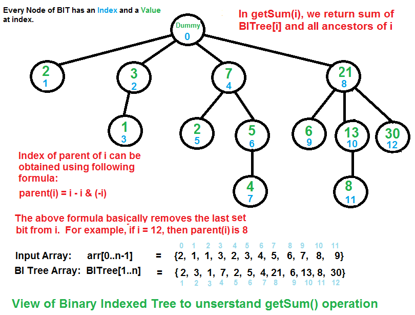
On the picture below you may see animated example of
creation of binary indexed tree for the
array `[1, 2, 3, 4, 5]` by inserting one by one.

## References
- [Wikipedia](https://en.wikipedia.org/wiki/Fenwick_tree)
- [GeeksForGeeks](https://www.geeksforgeeks.org/binary-indexed-tree-or-fenwick-tree-2/)
- [YouTube](https://www.youtube.com/watch?v=CWDQJGaN1gY&index=18&t=0s&list=PLLXdhg_r2hKA7DPDsunoDZ-Z769jWn4R8)
================================================
FILE: src/data-structures/tree/fenwick-tree/README.pt-BR.md
================================================
# Árvore Fenwick / Árvore Binária Indexada (Fenwick Tree / Binary Indexed Tree)
Uma **árvore Fenwick** ou **árvore binária indexada** é um tipo de
estrutura de dados que consegue eficiemente atualizar elementos e
calcular soma dos prefixos em uma tabela de números.
Quando comparado com um _flat array_ de números, a árvore Fenwick
alcança um balanceamento muito melhor entre duas operações: atualização
(_update_) do elemento e cálculo da soma do prefíxo. Em uma _flar array_
de `n` números, você pode tanto armazenar elementos quando a soma dos
prefixos. Em ambos os casos, computar a soma dos prefixos requer ou
atualizar um array de elementos também requerem um tempo linear, contudo,
a demais operações podem ser realizadas com tempo constante.
A árvore Fenwick permite ambas as operações serem realizadas com tempo
`O(log n)`.
Isto é possível devido a representação dos números como uma árvore, aonde
os valores de cada nó é a soma dos números naquela sub-árvore. A estrutura
de árvore permite operações a serem realizadas consumindo somente acessos
a nós em `O(log n)`.
## Implementação de Nós
Árvore Binária Indexada é representada como um _array_. Em cada nó da Árvore
Binária Indexada armazena a soma de alguns dos elementos de uma _array_
fornecida. O tamanho da Árvore Binária Indexada é igual a `n` aonde `n` é o
tamanho do _array_ de entrada. Na presente implementação nós utilizados o
tamanho `n+1` para uma implementação fácil. Todos os índices são baseados em 1.

Na imagem abaixo você pode ver o exemplo animado da criação de uma árvore
binária indexada para o _array_ `[1, 2, 3, 4, 5]`, sendo inseridos um após
o outro.

## Referências
- [Wikipedia](https://en.wikipedia.org/wiki/Fenwick_tree)
- [GeeksForGeeks](https://www.geeksforgeeks.org/binary-indexed-tree-or-fenwick-tree-2/)
- [YouTube](https://www.youtube.com/watch?v=CWDQJGaN1gY&index=18&t=0s&list=PLLXdhg_r2hKA7DPDsunoDZ-Z769jWn4R8)
================================================
FILE: src/data-structures/tree/fenwick-tree/__test__/FenwickTree.test.js
================================================
import FenwickTree from '../FenwickTree';
describe('FenwickTree', () => {
it('should create empty fenwick tree of correct size', () => {
const tree1 = new FenwickTree(5);
expect(tree1.treeArray.length).toBe(5 + 1);
for (let i = 0; i < 5; i += 1) {
expect(tree1.treeArray[i]).toBe(0);
}
const tree2 = new FenwickTree(50);
expect(tree2.treeArray.length).toBe(50 + 1);
});
it('should create correct fenwick tree', () => {
const inputArray = [3, 2, -1, 6, 5, 4, -3, 3, 7, 2, 3];
const tree = new FenwickTree(inputArray.length);
expect(tree.treeArray.length).toBe(inputArray.length + 1);
inputArray.forEach((value, index) => {
tree.increase(index + 1, value);
});
expect(tree.treeArray).toEqual([0, 3, 5, -1, 10, 5, 9, -3, 19, 7, 9, 3]);
expect(tree.query(1)).toBe(3);
expect(tree.query(2)).toBe(5);
expect(tree.query(3)).toBe(4);
expect(tree.query(4)).toBe(10);
expect(tree.query(5)).toBe(15);
expect(tree.query(6)).toBe(19);
expect(tree.query(7)).toBe(16);
expect(tree.query(8)).toBe(19);
expect(tree.query(9)).toBe(26);
expect(tree.query(10)).toBe(28);
expect(tree.query(11)).toBe(31);
expect(tree.queryRange(1, 1)).toBe(3);
expect(tree.queryRange(1, 2)).toBe(5);
expect(tree.queryRange(2, 4)).toBe(7);
expect(tree.queryRange(6, 9)).toBe(11);
tree.increase(3, 1);
expect(tree.query(1)).toBe(3);
expect(tree.query(2)).toBe(5);
expect(tree.query(3)).toBe(5);
expect(tree.query(4)).toBe(11);
expect(tree.query(5)).toBe(16);
expect(tree.query(6)).toBe(20);
expect(tree.query(7)).toBe(17);
expect(tree.query(8)).toBe(20);
expect(tree.query(9)).toBe(27);
expect(tree.query(10)).toBe(29);
expect(tree.query(11)).toBe(32);
expect(tree.queryRange(1, 1)).toBe(3);
expect(tree.queryRange(1, 2)).toBe(5);
expect(tree.queryRange(2, 4)).toBe(8);
expect(tree.queryRange(6, 9)).toBe(11);
});
it('should correctly execute queries', () => {
const tree = new FenwickTree(5);
tree.increase(1, 4);
tree.increase(3, 7);
expect(tree.query(1)).toBe(4);
expect(tree.query(3)).toBe(11);
expect(tree.query(5)).toBe(11);
expect(tree.queryRange(2, 3)).toBe(7);
tree.increase(2, 5);
expect(tree.query(5)).toBe(16);
tree.increase(1, 3);
expect(tree.queryRange(1, 1)).toBe(7);
expect(tree.query(5)).toBe(19);
expect(tree.queryRange(1, 5)).toBe(19);
});
it('should throw exceptions', () => {
const tree = new FenwickTree(5);
const increaseAtInvalidLowIndex = () => {
tree.increase(0, 1);
};
const increaseAtInvalidHighIndex = () => {
tree.increase(10, 1);
};
const queryInvalidLowIndex = () => {
tree.query(0);
};
const queryInvalidHighIndex = () => {
tree.query(10);
};
const rangeQueryInvalidIndex = () => {
tree.queryRange(3, 2);
};
expect(increaseAtInvalidLowIndex).toThrow();
expect(increaseAtInvalidHighIndex).toThrow();
expect(queryInvalidLowIndex).toThrow();
expect(queryInvalidHighIndex).toThrow();
expect(rangeQueryInvalidIndex).toThrow();
});
});
================================================
FILE: src/data-structures/tree/red-black-tree/README.md
================================================
# Red–Black Tree
_Read this in other languages:_
[_Português_](README.pt-BR.md)
A **red–black tree** is a kind of self-balancing binary search
tree in computer science. Each node of the binary tree has
an extra bit, and that bit is often interpreted as the
color (red or black) of the node. These color bits are used
to ensure the tree remains approximately balanced during
insertions and deletions.
Balance is preserved by painting each node of the tree with
one of two colors in a way that satisfies certain properties,
which collectively constrain how unbalanced the tree can
become in the worst case. When the tree is modified, the
new tree is subsequently rearranged and repainted to
restore the coloring properties. The properties are
designed in such a way that this rearranging and recoloring
can be performed efficiently.
The balancing of the tree is not perfect, but it is good
enough to allow it to guarantee searching in `O(log n)` time,
where `n` is the total number of elements in the tree.
The insertion and deletion operations, along with the tree
rearrangement and recoloring, are also performed
in `O(log n)` time.
An example of a red–black tree:

## Properties
In addition to the requirements imposed on a binary search
tree the following must be satisfied by a red–black tree:
- Each node is either red or black.
- The root is black. This rule is sometimes omitted.
Since the root can always be changed from red to black,
but not necessarily vice versa, this rule has little
effect on analysis.
- All leaves (NIL) are black.
- If a node is red, then both its children are black.
- Every path from a given node to any of its descendant
NIL nodes contains the same number of black nodes.
Some definitions: the number of black nodes from the root
to a node is the node's **black depth**; the uniform
number of black nodes in all paths from root to the leaves
is called the **black-height** of the red–black tree.
These constraints enforce a critical property of red–black
trees: _the path from the root to the farthest leaf is no more than twice as long as the path from the root to the nearest leaf_.
The result is that the tree is roughly height-balanced.
Since operations such as inserting, deleting, and finding
values require worst-case time proportional to the height
of the tree, this theoretical upper bound on the height
allows red–black trees to be efficient in the worst case,
unlike ordinary binary search trees.
## Balancing during insertion
### If uncle is RED
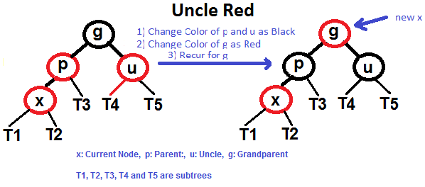
### If uncle is BLACK
- Left Left Case (`p` is left child of `g` and `x` is left child of `p`)
- Left Right Case (`p` is left child of `g` and `x` is right child of `p`)
- Right Right Case (`p` is right child of `g` and `x` is right child of `p`)
- Right Left Case (`p` is right child of `g` and `x` is left child of `p`)
#### Left Left Case (See g, p and x)
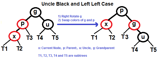
#### Left Right Case (See g, p and x)
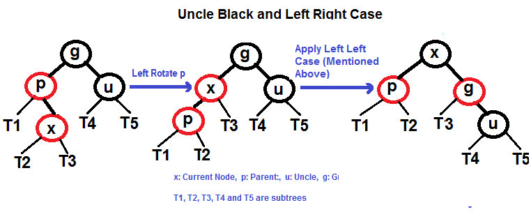
#### Right Right Case (See g, p and x)
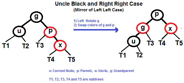
#### Right Left Case (See g, p and x)
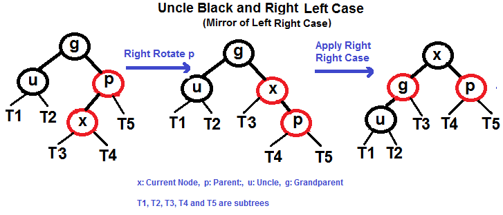
## References
- [Wikipedia](https://en.wikipedia.org/wiki/Red%E2%80%93black_tree)
- [Red Black Tree Insertion by Tushar Roy (YouTube)](https://www.youtube.com/watch?v=UaLIHuR1t8Q&list=PLLXdhg_r2hKA7DPDsunoDZ-Z769jWn4R8&index=63)
- [Red Black Tree Deletion by Tushar Roy (YouTube)](https://www.youtube.com/watch?v=CTvfzU_uNKE&t=0s&list=PLLXdhg_r2hKA7DPDsunoDZ-Z769jWn4R8&index=64)
- [Red Black Tree Insertion on GeeksForGeeks](https://www.geeksforgeeks.org/red-black-tree-set-2-insert/)
- [Red Black Tree Interactive Visualisations](https://www.cs.usfca.edu/~galles/visualization/RedBlack.html)
================================================
FILE: src/data-structures/tree/red-black-tree/README.pt-BR.md
================================================
# Árvore Vermelha-Preta (Red-Black Tree)
Uma **árvore vermelha-preta** é um tipo de árvore de pesquisa
binária auto balanceada na ciência da computação. Cada nó da
árvore binária possui um _bit_ extra, e este _bit_ é frequentemente
interpretado com a cor (vermelho ou preto) do nó. Estas cores de _bits_
são utilizadas para garantir que a árvore permanece aproximadamente
equilibrada durante as operações de inserções e remoções.
O equilíbrio é preservado através da pintura de cada nó da árvore com
uma das duas cores, de maneira que satisfaça certas propriedades, das
quais restringe nos piores dos casos, o quão desequilibrada a árvore
pode se tornar. Quando a árvore é modificada, a nova árvore é
subsequentemente reorganizada e repintada para restaurar as
propriedades de coloração. As propriedades são designadas de tal modo que
esta reorganização e nova pintura podem ser realizadas eficientemente.
O balanceamento de uma árvore não é perfeito, mas é suficientemente bom
para permitir e garantir uma pesquisa no tempo `O(log n)`, aonde `n` é o
número total de elementos na árvore.
Operações de inserções e remoções, juntamente com a reorganização e
repintura da árvore, também são executados no tempo `O (log n)`.
Um exemplo de uma árvore vermalha-preta:

## Propriedades
Em adição aos requerimentos impostos pela árvore de pesquisa binária,
as seguintes condições devem ser satisfeitas pela árvore vermelha-preta:
- Cada nó é tanto vermelho ou preto.
- O nó raíz é preto. Esta regra algumas vezes é omitida.
Tendo em vista que a raíz pode sempre ser alterada de vermelho para preto,
mas não de preto para vermelho, esta regra tem pouco efeito na análise.
- Todas as folhas (Nulo/NIL) são pretas.
- Caso um nó é vermelho, então seus filhos serão pretos.
- Cada caminho de um determinado nó para qualquer um dos seus nós nulos (NIL)
descendentes contém o mesmo número de nós pretos.
Algumas definições: o número de nós pretos da raiz até um nó é a
**profundidade preta**(_black depth_) do nó; o número uniforme de nós pretos
em todos os caminhos da raíz até as folhas são chamados de **altura negra**
(_black-height_) da árvore vermelha-preta.
Essas restrições impõem uma propriedade crítica de árvores vermelhas e pretas:
_o caminho da raiz até a folha mais distante não possui mais que o dobro do
comprimento do caminho da raiz até a folha mais próxima_.
O resultado é que a árvore é grosseiramente balanceada na altura.
Tendo em vista que operações como inserções, remoção e pesquisa de valores
requerem nos piores dos casos um tempo proporcional a altura da ávore,
este limite superior teórico na altura permite que as árvores vermelha-preta
sejam eficientes no pior dos casos, ao contrário das árvores de busca binária
comuns.
## Balanceamento durante a inserção
### Se o tio é VERMELHO

### Se o tio é PRETO
- Caso Esquerda Esquerda (`p` é o filho a esquerda de `g` e `x`, é o filho a esquerda de `p`)
- Caso Esquerda Direita (`p` é o filho a esquerda de `g` e `x`, é o filho a direita de `p`)
- Caso Direita Direita (`p` é o filho a direita de `g` e `x`, é o filho da direita de `p`)
- Caso Direita Esqueda (`p` é o filho a direita de `g` e `x`, é o filho a esquerda de `p`)
#### Caso Esquerda Esquerda (Veja g, p e x)

#### Caso Esquerda Direita (Veja g, p e x)

#### Caso Direita Direita (Veja g, p e x)

#### Caso Direita Esquerda (Veja g, p e x)

## Referências
- [Wikipedia](https://en.wikipedia.org/wiki/Red%E2%80%93black_tree)
- [Red Black Tree Insertion by Tushar Roy (YouTube)](https://www.youtube.com/watch?v=UaLIHuR1t8Q&list=PLLXdhg_r2hKA7DPDsunoDZ-Z769jWn4R8&index=63)
- [Red Black Tree Deletion by Tushar Roy (YouTube)](https://www.youtube.com/watch?v=CTvfzU_uNKE&t=0s&list=PLLXdhg_r2hKA7DPDsunoDZ-Z769jWn4R8&index=64)
- [Red Black Tree Insertion on GeeksForGeeks](https://www.geeksforgeeks.org/red-black-tree-set-2-insert/)
- [Red Black Tree Interactive Visualisations](https://www.cs.usfca.edu/~galles/visualization/RedBlack.html)
================================================
FILE: src/data-structures/tree/red-black-tree/RedBlackTree.js
================================================
import BinarySearchTree from '../binary-search-tree/BinarySearchTree';
// Possible colors of red-black tree nodes.
const RED_BLACK_TREE_COLORS = {
red: 'red',
black: 'black',
};
// Color property name in meta information of the nodes.
const COLOR_PROP_NAME = 'color';
export default class RedBlackTree extends BinarySearchTree {
/**
* @param {*} value
* @return {BinarySearchTreeNode}
*/
insert(value) {
const insertedNode = super.insert(value);
// if (!this.root.left && !this.root.right) {
if (this.nodeComparator.equal(insertedNode, this.root)) {
// Make root to always be black.
this.makeNodeBlack(insertedNode);
} else {
// Make all newly inserted nodes to be red.
this.makeNodeRed(insertedNode);
}
// Check all conditions and balance the node.
this.balance(insertedNode);
return insertedNode;
}
/**
* @param {*} value
* @return {boolean}
*/
remove(value) {
throw new Error(`Can't remove ${value}. Remove method is not implemented yet`);
}
/**
* @param {BinarySearchTreeNode} node
*/
balance(node) {
// If it is a root node then nothing to balance here.
if (this.nodeComparator.equal(node, this.root)) {
return;
}
// If the parent is black then done. Nothing to balance here.
if (this.isNodeBlack(node.parent)) {
return;
}
const grandParent = node.parent.parent;
if (node.uncle && this.isNodeRed(node.uncle)) {
// If node has red uncle then we need to do RECOLORING.
// Recolor parent and uncle to black.
this.makeNodeBlack(node.uncle);
this.makeNodeBlack(node.parent);
if (!this.nodeComparator.equal(grandParent, this.root)) {
// Recolor grand-parent to red if it is not root.
this.makeNodeRed(grandParent);
} else {
// If grand-parent is black root don't do anything.
// Since root already has two black sibling that we've just recolored.
return;
}
// Now do further checking for recolored grand-parent.
this.balance(grandParent);
} else if (!node.uncle || this.isNodeBlack(node.uncle)) {
// If node uncle is black or absent then we need to do ROTATIONS.
if (grandParent) {
// Grand parent that we will receive after rotations.
let newGrandParent;
if (this.nodeComparator.equal(grandParent.left, node.parent)) {
// Left case.
if (this.nodeComparator.equal(node.parent.left, node)) {
// Left-left case.
newGrandParent = this.leftLeftRotation(grandParent);
} else {
// Left-right case.
newGrandParent = this.leftRightRotation(grandParent);
}
} else {
// Right case.
if (this.nodeComparator.equal(node.parent.right, node)) {
// Right-right case.
newGrandParent = this.rightRightRotation(grandParent);
} else {
// Right-left case.
newGrandParent = this.rightLeftRotation(grandParent);
}
}
// Set newGrandParent as a root if it doesn't have parent.
if (newGrandParent && newGrandParent.parent === null) {
this.root = newGrandParent;
// Recolor root into black.
this.makeNodeBlack(this.root);
}
// Check if new grand parent don't violate red-black-tree rules.
this.balance(newGrandParent);
}
}
}
/**
* Left Left Case (p is left child of g and x is left child of p)
* @param {BinarySearchTreeNode|BinaryTreeNode} grandParentNode
* @return {BinarySearchTreeNode}
*/
leftLeftRotation(grandParentNode) {
// Memorize the parent of grand-parent node.
const grandGrandParent = grandParentNode.parent;
// Check what type of sibling is our grandParentNode is (left or right).
let grandParentNodeIsLeft;
if (grandGrandParent) {
grandParentNodeIsLeft = this.nodeComparator.equal(grandGrandParent.left, grandParentNode);
}
// Memorize grandParentNode's left node.
const parentNode = grandParentNode.left;
// Memorize parent's right node since we're going to transfer it to
// grand parent's left subtree.
const parentRightNode = parentNode.right;
// Make grandParentNode to be right child of parentNode.
parentNode.setRight(grandParentNode);
// Move child's right subtree to grandParentNode's left subtree.
grandParentNode.setLeft(parentRightNode);
// Put parentNode node in place of grandParentNode.
if (grandGrandParent) {
if (grandParentNodeIsLeft) {
grandGrandParent.setLeft(parentNode);
} else {
grandGrandParent.setRight(parentNode);
}
} else {
// Make parent node a root
parentNode.parent = null;
}
// Swap colors of grandParentNode and parentNode.
this.swapNodeColors(parentNode, grandParentNode);
// Return new root node.
return parentNode;
}
/**
* Left Right Case (p is left child of g and x is right child of p)
* @param {BinarySearchTreeNode|BinaryTreeNode} grandParentNode
* @return {BinarySearchTreeNode}
*/
leftRightRotation(grandParentNode) {
// Memorize left and left-right nodes.
const parentNode = grandParentNode.left;
const childNode = parentNode.right;
// We need to memorize child left node to prevent losing
// left child subtree. Later it will be re-assigned to
// parent's right sub-tree.
const childLeftNode = childNode.left;
// Make parentNode to be a left child of childNode node.
childNode.setLeft(parentNode);
// Move child's left subtree to parent's right subtree.
parentNode.setRight(childLeftNode);
// Put left-right node in place of left node.
grandParentNode.setLeft(childNode);
// Now we're ready to do left-left rotation.
return this.leftLeftRotation(grandParentNode);
}
/**
* Right Right Case (p is right child of g and x is right child of p)
* @param {BinarySearchTreeNode|BinaryTreeNode} grandParentNode
* @return {BinarySearchTreeNode}
*/
rightRightRotation(grandParentNode) {
// Memorize the parent of grand-parent node.
const grandGrandParent = grandParentNode.parent;
// Check what type of sibling is our grandParentNode is (left or right).
let grandParentNodeIsLeft;
if (grandGrandParent) {
grandParentNodeIsLeft = this.nodeComparator.equal(grandGrandParent.left, grandParentNode);
}
// Memorize grandParentNode's right node.
const parentNode = grandParentNode.right;
// Memorize parent's left node since we're going to transfer it to
// grand parent's right subtree.
const parentLeftNode = parentNode.left;
// Make grandParentNode to be left child of parentNode.
parentNode.setLeft(grandParentNode);
// Transfer all left nodes from parent to right sub-tree of grandparent.
grandParentNode.setRight(parentLeftNode);
// Put parentNode node in place of grandParentNode.
if (grandGrandParent) {
if (grandParentNodeIsLeft) {
grandGrandParent.setLeft(parentNode);
} else {
grandGrandParent.setRight(parentNode);
}
} else {
// Make parent node a root.
parentNode.parent = null;
}
// Swap colors of granParent and parent nodes.
this.swapNodeColors(parentNode, grandParentNode);
// Return new root node.
return parentNode;
}
/**
* Right Left Case (p is right child of g and x is left child of p)
* @param {BinarySearchTreeNode|BinaryTreeNode} grandParentNode
* @return {BinarySearchTreeNode}
*/
rightLeftRotation(grandParentNode) {
// Memorize right and right-left nodes.
const parentNode = grandParentNode.right;
const childNode = parentNode.left;
// We need to memorize child right node to prevent losing
// right child subtree. Later it will be re-assigned to
// parent's left sub-tree.
const childRightNode = childNode.right;
// Make parentNode to be a right child of childNode.
childNode.setRight(parentNode);
// Move child's right subtree to parent's left subtree.
parentNode.setLeft(childRightNode);
// Put childNode node in place of parentNode.
grandParentNode.setRight(childNode);
// Now we're ready to do right-right rotation.
return this.rightRightRotation(grandParentNode);
}
/**
* @param {BinarySearchTreeNode|BinaryTreeNode} node
* @return {BinarySearchTreeNode}
*/
makeNodeRed(node) {
node.meta.set(COLOR_PROP_NAME, RED_BLACK_TREE_COLORS.red);
return node;
}
/**
* @param {BinarySearchTreeNode|BinaryTreeNode} node
* @return {BinarySearchTreeNode}
*/
makeNodeBlack(node) {
node.meta.set(COLOR_PROP_NAME, RED_BLACK_TREE_COLORS.black);
return node;
}
/**
* @param {BinarySearchTreeNode|BinaryTreeNode} node
* @return {boolean}
*/
isNodeRed(node) {
return node.meta.get(COLOR_PROP_NAME) === RED_BLACK_TREE_COLORS.red;
}
/**
* @param {BinarySearchTreeNode|BinaryTreeNode} node
* @return {boolean}
*/
isNodeBlack(node) {
return node.meta.get(COLOR_PROP_NAME) === RED_BLACK_TREE_COLORS.black;
}
/**
* @param {BinarySearchTreeNode|BinaryTreeNode} node
* @return {boolean}
*/
isNodeColored(node) {
return this.isNodeRed(node) || this.isNodeBlack(node);
}
/**
* @param {BinarySearchTreeNode|BinaryTreeNode} firstNode
* @param {BinarySearchTreeNode|BinaryTreeNode} secondNode
*/
swapNodeColors(firstNode, secondNode) {
const firstColor = firstNode.meta.get(COLOR_PROP_NAME);
const secondColor = secondNode.meta.get(COLOR_PROP_NAME);
firstNode.meta.set(COLOR_PROP_NAME, secondColor);
secondNode.meta.set(COLOR_PROP_NAME, firstColor);
}
}
================================================
FILE: src/data-structures/tree/red-black-tree/__test__/RedBlackTree.test.js
================================================
import RedBlackTree from '../RedBlackTree';
describe('RedBlackTree', () => {
it('should always color first inserted node as black', () => {
const tree = new RedBlackTree();
const firstInsertedNode = tree.insert(10);
expect(tree.isNodeColored(firstInsertedNode)).toBe(true);
expect(tree.isNodeBlack(firstInsertedNode)).toBe(true);
expect(tree.isNodeRed(firstInsertedNode)).toBe(false);
expect(tree.toString()).toBe('10');
expect(tree.root.height).toBe(0);
});
it('should always color new leaf node as red', () => {
const tree = new RedBlackTree();
const firstInsertedNode = tree.insert(10);
const secondInsertedNode = tree.insert(15);
const thirdInsertedNode = tree.insert(5);
expect(tree.isNodeBlack(firstInsertedNode)).toBe(true);
expect(tree.isNodeRed(secondInsertedNode)).toBe(true);
expect(tree.isNodeRed(thirdInsertedNode)).toBe(true);
expect(tree.toString()).toBe('5,10,15');
expect(tree.root.height).toBe(1);
});
it('should balance itself', () => {
const tree = new RedBlackTree();
tree.insert(5);
tree.insert(10);
tree.insert(15);
tree.insert(20);
tree.insert(25);
tree.insert(30);
expect(tree.toString()).toBe('5,10,15,20,25,30');
expect(tree.root.height).toBe(3);
});
it('should balance itself when parent is black', () => {
const tree = new RedBlackTree();
const node1 = tree.insert(10);
expect(tree.isNodeBlack(node1)).toBe(true);
const node2 = tree.insert(-10);
expect(tree.isNodeBlack(node1)).toBe(true);
expect(tree.isNodeRed(node2)).toBe(true);
const node3 = tree.insert(20);
expect(tree.isNodeBlack(node1)).toBe(true);
expect(tree.isNodeRed(node2)).toBe(true);
expect(tree.isNodeRed(node3)).toBe(true);
const node4 = tree.insert(-20);
expect(tree.isNodeBlack(node1)).toBe(true);
expect(tree.isNodeBlack(node2)).toBe(true);
expect(tree.isNodeBlack(node3)).toBe(true);
expect(tree.isNodeRed(node4)).toBe(true);
const node5 = tree.insert(25);
expect(tree.isNodeBlack(node1)).toBe(true);
expect(tree.isNodeBlack(node2)).toBe(true);
expect(tree.isNodeBlack(node3)).toBe(true);
expect(tree.isNodeRed(node4)).toBe(true);
expect(tree.isNodeRed(node5)).toBe(true);
const node6 = tree.insert(6);
expect(tree.isNodeBlack(node1)).toBe(true);
expect(tree.isNodeBlack(node2)).toBe(true);
expect(tree.isNodeBlack(node3)).toBe(true);
expect(tree.isNodeRed(node4)).toBe(true);
expect(tree.isNodeRed(node5)).toBe(true);
expect(tree.isNodeRed(node6)).toBe(true);
expect(tree.toString()).toBe('-20,-10,6,10,20,25');
expect(tree.root.height).toBe(2);
const node7 = tree.insert(4);
expect(tree.root.left.value).toEqual(node2.value);
expect(tree.toString()).toBe('-20,-10,4,6,10,20,25');
expect(tree.root.height).toBe(3);
expect(tree.isNodeBlack(node1)).toBe(true);
expect(tree.isNodeRed(node2)).toBe(true);
expect(tree.isNodeBlack(node3)).toBe(true);
expect(tree.isNodeBlack(node4)).toBe(true);
expect(tree.isNodeBlack(node4)).toBe(true);
expect(tree.isNodeRed(node5)).toBe(true);
expect(tree.isNodeBlack(node6)).toBe(true);
expect(tree.isNodeRed(node7)).toBe(true);
});
it('should balance itself when uncle is red', () => {
const tree = new RedBlackTree();
const node1 = tree.insert(10);
const node2 = tree.insert(-10);
const node3 = tree.insert(20);
const node4 = tree.insert(-20);
const node5 = tree.insert(6);
const node6 = tree.insert(15);
const node7 = tree.insert(25);
const node8 = tree.insert(2);
const node9 = tree.insert(8);
expect(tree.toString()).toBe('-20,-10,2,6,8,10,15,20,25');
expect(tree.root.height).toBe(3);
expect(tree.isNodeBlack(node1)).toBe(true);
expect(tree.isNodeRed(node2)).toBe(true);
expect(tree.isNodeBlack(node3)).toBe(true);
expect(tree.isNodeBlack(node4)).toBe(true);
expect(tree.isNodeBlack(node5)).toBe(true);
expect(tree.isNodeRed(node6)).toBe(true);
expect(tree.isNodeRed(node7)).toBe(true);
expect(tree.isNodeRed(node8)).toBe(true);
expect(tree.isNodeRed(node9)).toBe(true);
const node10 = tree.insert(4);
expect(tree.toString()).toBe('-20,-10,2,4,6,8,10,15,20,25');
expect(tree.root.height).toBe(3);
expect(tree.root.value).toBe(node5.value);
expect(tree.isNodeBlack(node5)).toBe(true);
expect(tree.isNodeRed(node1)).toBe(true);
expect(tree.isNodeRed(node2)).toBe(true);
expect(tree.isNodeRed(node10)).toBe(true);
expect(tree.isNodeRed(node6)).toBe(true);
expect(tree.isNodeRed(node7)).toBe(true);
expect(tree.isNodeBlack(node4)).toBe(true);
expect(tree.isNodeBlack(node8)).toBe(true);
expect(tree.isNodeBlack(node9)).toBe(true);
expect(tree.isNodeBlack(node3)).toBe(true);
});
it('should do left-left rotation', () => {
const tree = new RedBlackTree();
const node1 = tree.insert(10);
const node2 = tree.insert(-10);
const node3 = tree.insert(20);
const node4 = tree.insert(7);
const node5 = tree.insert(15);
expect(tree.toString()).toBe('-10,7,10,15,20');
expect(tree.root.height).toBe(2);
expect(tree.isNodeBlack(node1)).toBe(true);
expect(tree.isNodeBlack(node2)).toBe(true);
expect(tree.isNodeBlack(node3)).toBe(true);
expect(tree.isNodeRed(node4)).toBe(true);
expect(tree.isNodeRed(node5)).toBe(true);
const node6 = tree.insert(13);
expect(tree.toString()).toBe('-10,7,10,13,15,20');
expect(tree.root.height).toBe(2);
expect(tree.isNodeBlack(node1)).toBe(true);
expect(tree.isNodeBlack(node2)).toBe(true);
expect(tree.isNodeBlack(node5)).toBe(true);
expect(tree.isNodeRed(node4)).toBe(true);
expect(tree.isNodeRed(node6)).toBe(true);
expect(tree.isNodeRed(node3)).toBe(true);
});
it('should do left-right rotation', () => {
const tree = new RedBlackTree();
const node1 = tree.insert(10);
const node2 = tree.insert(-10);
const node3 = tree.insert(20);
const node4 = tree.insert(7);
const node5 = tree.insert(15);
expect(tree.toString()).toBe('-10,7,10,15,20');
expect(tree.root.height).toBe(2);
expect(tree.isNodeBlack(node1)).toBe(true);
expect(tree.isNodeBlack(node2)).toBe(true);
expect(tree.isNodeBlack(node3)).toBe(true);
expect(tree.isNodeRed(node4)).toBe(true);
expect(tree.isNodeRed(node5)).toBe(true);
const node6 = tree.insert(17);
expect(tree.toString()).toBe('-10,7,10,15,17,20');
expect(tree.root.height).toBe(2);
expect(tree.isNodeBlack(node1)).toBe(true);
expect(tree.isNodeBlack(node2)).toBe(true);
expect(tree.isNodeBlack(node6)).toBe(true);
expect(tree.isNodeRed(node4)).toBe(true);
expect(tree.isNodeRed(node5)).toBe(true);
expect(tree.isNodeRed(node3)).toBe(true);
});
it('should do recoloring, left-left and left-right rotation', () => {
const tree = new RedBlackTree();
const node1 = tree.insert(10);
const node2 = tree.insert(-10);
const node3 = tree.insert(20);
const node4 = tree.insert(-20);
const node5 = tree.insert(6);
const node6 = tree.insert(15);
const node7 = tree.insert(30);
const node8 = tree.insert(1);
const node9 = tree.insert(9);
expect(tree.toString()).toBe('-20,-10,1,6,9,10,15,20,30');
expect(tree.root.height).toBe(3);
expect(tree.isNodeBlack(node1)).toBe(true);
expect(tree.isNodeRed(node2)).toBe(true);
expect(tree.isNodeBlack(node3)).toBe(true);
expect(tree.isNodeBlack(node4)).toBe(true);
expect(tree.isNodeBlack(node5)).toBe(true);
expect(tree.isNodeRed(node6)).toBe(true);
expect(tree.isNodeRed(node7)).toBe(true);
expect(tree.isNodeRed(node8)).toBe(true);
expect(tree.isNodeRed(node9)).toBe(true);
tree.insert(4);
expect(tree.toString()).toBe('-20,-10,1,4,6,9,10,15,20,30');
expect(tree.root.height).toBe(3);
});
it('should do right-left rotation', () => {
const tree = new RedBlackTree();
const node1 = tree.insert(10);
const node2 = tree.insert(-10);
const node3 = tree.insert(20);
const node4 = tree.insert(-20);
const node5 = tree.insert(6);
const node6 = tree.insert(30);
expect(tree.toString()).toBe('-20,-10,6,10,20,30');
expect(tree.root.height).toBe(2);
expect(tree.isNodeBlack(node1)).toBe(true);
expect(tree.isNodeBlack(node2)).toBe(true);
expect(tree.isNodeBlack(node3)).toBe(true);
expect(tree.isNodeRed(node4)).toBe(true);
expect(tree.isNodeRed(node5)).toBe(true);
expect(tree.isNodeRed(node6)).toBe(true);
const node7 = tree.insert(25);
const rightNode = tree.root.right;
const rightLeftNode = rightNode.left;
const rightRightNode = rightNode.right;
expect(rightNode.value).toBe(node7.value);
expect(rightLeftNode.value).toBe(node3.value);
expect(rightRightNode.value).toBe(node6.value);
expect(tree.toString()).toBe('-20,-10,6,10,20,25,30');
expect(tree.root.height).toBe(2);
expect(tree.isNodeBlack(node1)).toBe(true);
expect(tree.isNodeBlack(node2)).toBe(true);
expect(tree.isNodeBlack(node7)).toBe(true);
expect(tree.isNodeRed(node4)).toBe(true);
expect(tree.isNodeRed(node5)).toBe(true);
expect(tree.isNodeRed(node3)).toBe(true);
expect(tree.isNodeRed(node6)).toBe(true);
});
it('should do left-left rotation with left grand-parent', () => {
const tree = new RedBlackTree();
tree.insert(20);
tree.insert(15);
tree.insert(25);
tree.insert(10);
tree.insert(5);
expect(tree.toString()).toBe('5,10,15,20,25');
expect(tree.root.height).toBe(2);
});
it('should do right-right rotation with left grand-parent', () => {
const tree = new RedBlackTree();
tree.insert(20);
tree.insert(15);
tree.insert(25);
tree.insert(17);
tree.insert(19);
expect(tree.toString()).toBe('15,17,19,20,25');
expect(tree.root.height).toBe(2);
});
it('should throw an error when trying to remove node', () => {
const removeNodeFromRedBlackTree = () => {
const tree = new RedBlackTree();
tree.remove(1);
};
expect(removeNodeFromRedBlackTree).toThrow();
});
});
================================================
FILE: src/data-structures/tree/segment-tree/README.md
================================================
# Segment Tree
_Read this in other languages:_
[_Português_](README.pt-BR.md)
In computer science, a **segment tree** also known as a statistic tree
is a tree data structure used for storing information about intervals,
or segments. It allows querying which of the stored segments contain
a given point. It is, in principle, a static structure; that is,
it's a structure that cannot be modified once it's built. A similar
data structure is the interval tree.
A segment tree is a binary tree. The root of the tree represents the
whole array. The two children of the root represent the
first and second halves of the array. Similarly, the
children of each node corresponds to the two halves of
the array corresponding to the node.
We build the tree bottom up, with the value of each node
being the "minimum" (or any other function) of its children's values. This will
take `O(n log n)` time. The number
of operations done is the height of the tree, which
is `O(log n)`. To do range queries, each node splits the
query into two parts, one sub-query for each child.
If a query contains the whole subarray of a node, we
can use the precomputed value at the node. Using this
optimisation, we can prove that only `O(log n)` minimum
operations are done.
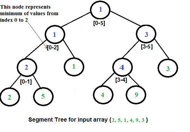

## Application
A segment tree is a data structure designed to perform
certain array operations efficiently - especially those
involving range queries.
Applications of the segment tree are in the areas of computational geometry,
and geographic information systems.
Current implementation of Segment Tree implies that you may
pass any binary (with two input params) function to it and
thus you're able to do range query for variety of functions.
In tests you may find examples of doing `min`, `max` and `sum` range
queries on SegmentTree.
## References
- [Wikipedia](https://en.wikipedia.org/wiki/Segment_tree)
- [YouTube](https://www.youtube.com/watch?v=ZBHKZF5w4YU&index=65&list=PLLXdhg_r2hKA7DPDsunoDZ-Z769jWn4R8)
- [GeeksForGeeks](https://www.geeksforgeeks.org/segment-tree-set-1-sum-of-given-range/)
================================================
FILE: src/data-structures/tree/segment-tree/README.pt-BR.md
================================================
# Árvore de Segmento (Segment Tree)
Na ciência da computação, uma **árvore de segmento** também conhecida como
árvore estatística é uma árvore de estrutura de dados utilizadas para
armazenar informações sobre intervalores ou segmentos. Ela permite pesquisas
no qual os segmentos armazenados contém um ponto fornecido. Isto é,
em princípio, uma estrutura estática; ou seja, é uma estrutura que não pode
ser modificada depois de inicializada. Uma estrutura de dados similar é a
árvore de intervalos.
Uma árvore de segmento é uma árvore binária. A raíz da árvore representa a
_array_ inteira. Os dois filhos da raíz representam a primeira e a segunda
metade da _array_. Similarmente, os filhos de cada nó correspondem ao número
das duas metadas da _array_ correspondente do nó.
Nós construímos a árvore debaixo para cima, com o valor de cada nó sendo o
"mínimo" (ou qualquer outra função) dos valores de seus filhos. Isto consumirá
tempo `O(n log n)`. O número de oprações realizadas é equivalente a altura da
árvore, pela qual consome tempo `O(log n)`. Para fazer consultas de intervalos,
cada nó divide a consulta em duas partes, sendo uma sub consulta para cada filho.
Se uma pesquisa contém todo o _subarray_ de um nó, nós podemos utilizar do valor
pré-calculado do nó. Utilizando esta otimização, nós podemos provar que somente
operações mínimas `O(log n)` são realizadas.


## Aplicação
Uma árvore de segmento é uma estrutura de dados designada a realizar
certas operações de _array_ eficientemente, especialmente aquelas envolvendo
consultas de intervalos.
Aplicações da árvore de segmentos são nas áreas de computação geométrica e
sistemas de informação geográficos.
A implementação atual da Árvore de Segmentos implica que você pode passar
qualquer função binária (com dois parâmetros de entradas) e então, você
será capaz de realizar consultas de intervalos para uma variedade de funções.
Nos testes você poderá encontrar exemplos realizando `min`, `max` e consultas de
intervalo `sum` na árvore segmentada (SegmentTree).
## Referências
- [Wikipedia](https://en.wikipedia.org/wiki/Segment_tree)
- [YouTube](https://www.youtube.com/watch?v=ZBHKZF5w4YU&index=65&list=PLLXdhg_r2hKA7DPDsunoDZ-Z769jWn4R8)
- [GeeksForGeeks](https://www.geeksforgeeks.org/segment-tree-set-1-sum-of-given-range/)
================================================
FILE: src/data-structures/tree/segment-tree/SegmentTree.js
================================================
import isPowerOfTwo from '../../../algorithms/math/is-power-of-two/isPowerOfTwo';
export default class SegmentTree {
/**
* @param {number[]} inputArray
* @param {function} operation - binary function (i.e. sum, min)
* @param {number} operationFallback - operation fallback value (i.e. 0 for sum, Infinity for min)
*/
constructor(inputArray, operation, operationFallback) {
this.inputArray = inputArray;
this.operation = operation;
this.operationFallback = operationFallback;
// Init array representation of segment tree.
this.segmentTree = this.initSegmentTree(this.inputArray);
this.buildSegmentTree();
}
/**
* @param {number[]} inputArray
* @return {number[]}
*/
initSegmentTree(inputArray) {
let segmentTreeArrayLength;
const inputArrayLength = inputArray.length;
if (isPowerOfTwo(inputArrayLength)) {
// If original array length is a power of two.
segmentTreeArrayLength = (2 * inputArrayLength) - 1;
} else {
// If original array length is not a power of two then we need to find
// next number that is a power of two and use it to calculate
// tree array size. This is happens because we need to fill empty children
// in perfect binary tree with nulls.And those nulls need extra space.
const currentPower = Math.floor(Math.log2(inputArrayLength));
const nextPower = currentPower + 1;
const nextPowerOfTwoNumber = 2 ** nextPower;
segmentTreeArrayLength = (2 * nextPowerOfTwoNumber) - 1;
}
return new Array(segmentTreeArrayLength).fill(null);
}
/**
* Build segment tree.
*/
buildSegmentTree() {
const leftIndex = 0;
const rightIndex = this.inputArray.length - 1;
const position = 0;
this.buildTreeRecursively(leftIndex, rightIndex, position);
}
/**
* Build segment tree recursively.
*
* @param {number} leftInputIndex
* @param {number} rightInputIndex
* @param {number} position
*/
buildTreeRecursively(leftInputIndex, rightInputIndex, position) {
// If low input index and high input index are equal that would mean
// the we have finished splitting and we are already came to the leaf
// of the segment tree. We need to copy this leaf value from input
// array to segment tree.
if (leftInputIndex === rightInputIndex) {
this.segmentTree[position] = this.inputArray[leftInputIndex];
return;
}
// Split input array on two halves and process them recursively.
const middleIndex = Math.floor((leftInputIndex + rightInputIndex) / 2);
// Process left half of the input array.
this.buildTreeRecursively(leftInputIndex, middleIndex, this.getLeftChildIndex(position));
// Process right half of the input array.
this.buildTreeRecursively(middleIndex + 1, rightInputIndex, this.getRightChildIndex(position));
// Once every tree leaf is not empty we're able to build tree bottom up using
// provided operation function.
this.segmentTree[position] = this.operation(
this.segmentTree[this.getLeftChildIndex(position)],
this.segmentTree[this.getRightChildIndex(position)],
);
}
/**
* Do range query on segment tree in context of this.operation function.
*
* @param {number} queryLeftIndex
* @param {number} queryRightIndex
* @return {number}
*/
rangeQuery(queryLeftIndex, queryRightIndex) {
const leftIndex = 0;
const rightIndex = this.inputArray.length - 1;
const position = 0;
return this.rangeQueryRecursive(
queryLeftIndex,
queryRightIndex,
leftIndex,
rightIndex,
position,
);
}
/**
* Do range query on segment tree recursively in context of this.operation function.
*
* @param {number} queryLeftIndex - left index of the query
* @param {number} queryRightIndex - right index of the query
* @param {number} leftIndex - left index of input array segment
* @param {number} rightIndex - right index of input array segment
* @param {number} position - root position in binary tree
* @return {number}
*/
rangeQueryRecursive(queryLeftIndex, queryRightIndex, leftIndex, rightIndex, position) {
if (queryLeftIndex <= leftIndex && queryRightIndex >= rightIndex) {
// Total overlap.
return this.segmentTree[position];
}
if (queryLeftIndex > rightIndex || queryRightIndex < leftIndex) {
// No overlap.
return this.operationFallback;
}
// Partial overlap.
const middleIndex = Math.floor((leftIndex + rightIndex) / 2);
const leftOperationResult = this.rangeQueryRecursive(
queryLeftIndex,
queryRightIndex,
leftIndex,
middleIndex,
this.getLeftChildIndex(position),
);
const rightOperationResult = this.rangeQueryRecursive(
queryLeftIndex,
queryRightIndex,
middleIndex + 1,
rightIndex,
this.getRightChildIndex(position),
);
return this.operation(leftOperationResult, rightOperationResult);
}
/**
* Left child index.
* @param {number} parentIndex
* @return {number}
*/
getLeftChildIndex(parentIndex) {
return (2 * parentIndex) + 1;
}
/**
* Right child index.
* @param {number} parentIndex
* @return {number}
*/
getRightChildIndex(parentIndex) {
return (2 * parentIndex) + 2;
}
}
================================================
FILE: src/data-structures/tree/segment-tree/__test__/SegmentTree.test.js
================================================
import SegmentTree from '../SegmentTree';
describe('SegmentTree', () => {
it('should build tree for input array #0 with length of power of two', () => {
const array = [-1, 2];
const segmentTree = new SegmentTree(array, Math.min, Infinity);
expect(segmentTree.segmentTree).toEqual([-1, -1, 2]);
expect(segmentTree.segmentTree.length).toBe((2 * array.length) - 1);
});
it('should build tree for input array #1 with length of power of two', () => {
const array = [-1, 2, 4, 0];
const segmentTree = new SegmentTree(array, Math.min, Infinity);
expect(segmentTree.segmentTree).toEqual([-1, -1, 0, -1, 2, 4, 0]);
expect(segmentTree.segmentTree.length).toBe((2 * array.length) - 1);
});
it('should build tree for input array #0 with length not of power of two', () => {
const array = [0, 1, 2];
const segmentTree = new SegmentTree(array, Math.min, Infinity);
expect(segmentTree.segmentTree).toEqual([0, 0, 2, 0, 1, null, null]);
expect(segmentTree.segmentTree.length).toBe((2 * 4) - 1);
});
it('should build tree for input array #1 with length not of power of two', () => {
const array = [-1, 3, 4, 0, 2, 1];
const segmentTree = new SegmentTree(array, Math.min, Infinity);
expect(segmentTree.segmentTree).toEqual([
-1, -1, 0, -1, 4, 0, 1, -1, 3, null, null, 0, 2, null, null,
]);
expect(segmentTree.segmentTree.length).toBe((2 * 8) - 1);
});
it('should build max array', () => {
const array = [-1, 2, 4, 0];
const segmentTree = new SegmentTree(array, Math.max, -Infinity);
expect(segmentTree.segmentTree).toEqual([4, 2, 4, -1, 2, 4, 0]);
expect(segmentTree.segmentTree.length).toBe((2 * array.length) - 1);
});
it('should build sum array', () => {
const array = [-1, 2, 4, 0];
const segmentTree = new SegmentTree(array, (a, b) => (a + b), 0);
expect(segmentTree.segmentTree).toEqual([5, 1, 4, -1, 2, 4, 0]);
expect(segmentTree.segmentTree.length).toBe((2 * array.length) - 1);
});
it('should do min range query on power of two length array', () => {
const array = [-1, 3, 4, 0, 2, 1];
const segmentTree = new SegmentTree(array, Math.min, Infinity);
expect(segmentTree.rangeQuery(0, 5)).toBe(-1);
expect(segmentTree.rangeQuery(0, 2)).toBe(-1);
expect(segmentTree.rangeQuery(1, 3)).toBe(0);
expect(segmentTree.rangeQuery(2, 4)).toBe(0);
expect(segmentTree.rangeQuery(4, 5)).toBe(1);
expect(segmentTree.rangeQuery(2, 2)).toBe(4);
});
it('should do min range query on not power of two length array', () => {
const array = [-1, 2, 4, 0];
const segmentTree = new SegmentTree(array, Math.min, Infinity);
expect(segmentTree.rangeQuery(0, 4)).toBe(-1);
expect(segmentTree.rangeQuery(0, 1)).toBe(-1);
expect(segmentTree.rangeQuery(1, 3)).toBe(0);
expect(segmentTree.rangeQuery(1, 2)).toBe(2);
expect(segmentTree.rangeQuery(2, 3)).toBe(0);
expect(segmentTree.rangeQuery(2, 2)).toBe(4);
});
it('should do max range query', () => {
const array = [-1, 3, 4, 0, 2, 1];
const segmentTree = new SegmentTree(array, Math.max, -Infinity);
expect(segmentTree.rangeQuery(0, 5)).toBe(4);
expect(segmentTree.rangeQuery(0, 1)).toBe(3);
expect(segmentTree.rangeQuery(1, 3)).toBe(4);
expect(segmentTree.rangeQuery(2, 4)).toBe(4);
expect(segmentTree.rangeQuery(4, 5)).toBe(2);
expect(segmentTree.rangeQuery(3, 3)).toBe(0);
});
it('should do sum range query', () => {
const array = [-1, 3, 4, 0, 2, 1];
const segmentTree = new SegmentTree(array, (a, b) => (a + b), 0);
expect(segmentTree.rangeQuery(0, 5)).toBe(9);
expect(segmentTree.rangeQuery(0, 1)).toBe(2);
expect(segmentTree.rangeQuery(1, 3)).toBe(7);
expect(segmentTree.rangeQuery(2, 4)).toBe(6);
expect(segmentTree.rangeQuery(4, 5)).toBe(3);
expect(segmentTree.rangeQuery(3, 3)).toBe(0);
});
});
================================================
FILE: src/data-structures/trie/README.ko-KO.md
================================================
# Trie
_Read this in other languages:_
[_简体中文_](README.zh-CN.md),
[_Русский_](README.ru-RU.md),
[_Português_](README.pt-BR.md),
[_Українська_](README.uk-UA.md),
[_한국어_](README.ko-KO.md)
컴퓨터 과학에서 **트라이**는 디지털 트리라고도 불리며 때로는 기수 트리 또는 접두사 트리(접두사로 검색할 수 있기 때문에)라고도 불리며 일종의 검색 트리입니다. 키가 보통 문자열인 동적 집합 또는 연관 배열을 저장하는 데 사용되는 순서가 지정된 트리 데이터 구조입니다. 이진 검색 트리와 달리 트리의 어떤 노드도 해당 노드와 연결된 키를 저장하지 않으며 대신 트리의 위치가 해당 노드와 연결된 키를 정의합니다. 노드의 모든 하위 항목은 해당 노드와 연결된 문자열의 공통 접두사를 가지며 루트는 빈 문자열과 연결됩니다. 값은 모든 노드와 반드시 연결되지는 않습니다. 오히려 값은 나뭇잎과 관심 있는 키에 해당하는 일부 내부 노드에만 연결되는 경향이 있습니다. 접두사 트리의 공간에 최적화된 표현은 콤팩트 접두사 트리를 참조하십시오.

_Made with [okso.app](https://okso.app)_
## 참조
- [Wikipedia]()
- [YouTube](https://www.youtube.com/watch?v=zIjfhVPRZCg&list=PLLXdhg_r2hKA7DPDsunoDZ-Z769jWn4R8&index=7&t=0s)
================================================
FILE: src/data-structures/trie/README.md
================================================
# Trie
_Read this in other languages:_
[_简体中文_](README.zh-CN.md),
[_Русский_](README.ru-RU.md),
[_Português_](README.pt-BR.md),
[_Українська_](README.uk-UA.md),
[_한국어_](README.ko-KO.md)
In computer science, a **trie**, also called digital tree and sometimes
radix tree or prefix tree (as they can be searched by prefixes),
is a kind of search tree—an ordered tree data structure that is
used to store a dynamic set or associative array where the keys
are usually strings. Unlike a binary search tree, no node in the
tree stores the key associated with that node; instead, its
position in the tree defines the key with which it is associated.
All the descendants of a node have a common prefix of the string
associated with that node, and the root is associated with the
empty string. Values are not necessarily associated with every
node. Rather, values tend only to be associated with leaves,
and with some inner nodes that correspond to keys of interest.
For the space-optimized presentation of prefix tree, see compact
prefix tree.

*Made with [okso.app](https://okso.app)*
## References
- [Wikipedia](https://en.wikipedia.org/wiki/Trie)
- [YouTube](https://www.youtube.com/watch?v=zIjfhVPRZCg&list=PLLXdhg_r2hKA7DPDsunoDZ-Z769jWn4R8&index=7&t=0s)
================================================
FILE: src/data-structures/trie/README.pt-BR.md
================================================
# Árvore de Prefixos (Trie)
Na ciência da computação, uma **trie**, também chamada de árvore digital (digital tree)
e algumas vezes de _radix tree_ ou _prefix tree_ (tendo em vista que eles
podem ser pesquisados por prefixos), é um tipo de árvore de pesquisa, uma
estrutura de dados de árvore ordenada que é usado para armazenar um
conjunto dinâmico ou matriz associativa onde as chaves são geralmente _strings_.
Ao contrário de uma árvore de pesquisa binária (binary search tree),
nenhum nó na árvore armazena a chave associada a esse nó; em vez disso,
sua posição na árvore define a chave com a qual ela está associada.
Todos os descendentes de um nó possuem em comum o prefixo de uma _string_
associada com aquele nó, e a raiz é associada com uma _string_ vazia.
Valores não são necessariamente associados a todos nós. Em vez disso,
os valores tendem a ser associados apenas a folhas e com alguns nós
internos que correspondem a chaves de interesse.
Para a apresentação otimizada do espaço da árvore de prefixo (_prefix tree_),
veja árvore de prefixo compacto.

*Made with [okso.app](https://okso.app)*
## Referências
- [Wikipedia](https://en.wikipedia.org/wiki/Trie)
- [YouTube](https://www.youtube.com/watch?v=zIjfhVPRZCg&list=PLLXdhg_r2hKA7DPDsunoDZ-Z769jWn4R8&index=7&t=0s)
================================================
FILE: src/data-structures/trie/README.ru-RU.md
================================================
# Префиксное дерево
**Префиксное дерево** (также бор, луч, нагруженное или суффиксное дерево) в информатике - упорядоченная древовидная
структура данных, которая используется для хранения динамических множеств или ассоциативных массивов, где
ключом обычно выступают строки. Дерево называется префиксным, потому что поиск осуществляется по префиксам.
В отличие от бинарного дерева, узлы не содержат ключи, соответствующие узлу. Представляет собой корневое дерево, каждое
ребро которого помечено каким-то символом так, что для любого узла все рёбра, соединяющие этот узел с его сыновьями,
помечены разными символами. Некоторые узлы префиксного дерева выделены (на рисунке они подписаны цифрами) и считается,
что префиксное дерево содержит данную строку-ключ тогда и только тогда, когда эту строку можно прочитать на пути из
корня до некоторого выделенного узла.
Таким образом, в отличие от бинарных деревьев поиска, ключ, идентифицирующий конкретный узел дерева, не явно хранится в
данном узле, а неявно задаётся положением данного узла в дереве. Получить ключ можно выписыванием подряд символов,
помечающих рёбра на пути от корня до узла. Ключ корня дерева — пустая строка. Часто в выделенных узлах хранят
дополнительную информацию, связанную с ключом, и обычно выделенными являются только листья и, возможно, некоторые
внутренние узлы.

*Made with [okso.app](https://okso.app)*
На рисунке представлено префиксное дерево, содержащее ключи «A», «to», «tea», «ted», «ten», «i», «in», «inn».
## Ссылки
- [Wikipedia](https://ru.wikipedia.org/wiki/%D0%9F%D1%80%D0%B5%D1%84%D0%B8%D0%BA%D1%81%D0%BD%D0%BE%D0%B5_%D0%B4%D0%B5%D1%80%D0%B5%D0%B2%D0%BE)
- [YouTube](https://www.youtube.com/watch?v=zIjfhVPRZCg&list=PLLXdhg_r2hKA7DPDsunoDZ-Z769jWn4R8&index=7&t=0s)
================================================
FILE: src/data-structures/trie/README.uk-UA.md
================================================
# Префіксне дерево
**Префіксне дерево** (Також промінь, навантажене або суфіксне дерево) в інформатиці - впорядкована деревоподібна
структура даних, яка використовується для зберігання динамічних множин або асоціативних масивів, де
ключем зазвичай виступають рядки. Дерево називається префіксним, тому що пошук здійснюється за префіксами.
На відміну від бінарного дерева, вузли не містять ключів, що відповідають вузлу. Являє собою кореневе дерево, кожне
ребро якого позначено якимось символом так, що для будь-якого вузла всі ребра, що з'єднують цей вузол з його синами,
позначені різними символами. Деякі вузли префіксного дерева виділені (на малюнку вони підписані цифрами) і вважається,
що префіксне дерево містить цей рядок-ключ тоді і тільки тоді, коли цей рядок можна прочитати на шляху з
кореня до певного виділеного вузла.
Таким чином, на відміну від бінарних дерев пошуку, ключ, що ідентифікує конкретний вузол дерева, не явно зберігається в
цьому вузлі, а неявно задається положенням цього вузла в дереві. Отримати ключ можна виписуванням поспіль символів,
помічають ребра по дорозі від кореня до вузла. Ключ кореня дерева - порожній рядок. Часто у виділених вузлах зберігають
додаткову інформацію, пов'язану з ключем, і зазвичай виділеними є тільки листя і, можливо, деякі
внутрішні вузли.

*Made with [okso.app](https://okso.app)*
На малюнку представлено префіксне дерево, що містить ключі. «A», «to», «tea», «ted», «ten», «i», «in», «inn».
## Посилання
- [Wikipedia](https://uk.wikipedia.org/wiki/%D0%9F%D1%80%D0%B5%D1%84%D1%96%D0%BA%D1%81%D0%BD%D0%B5_%D0%B4%D0%B5%D1%80%D0%B5%D0%B2%D0%BE)
================================================
FILE: src/data-structures/trie/README.zh-CN.md
================================================
# 字典树
在计算机科学中, **字典树(trie,中文又被称为”单词查找树“或 ”键树“)**, 也称为数字树,有时候也被称为基数树或前缀树(因为它们可以通过前缀搜索),它是一种搜索树--一种已排序的数据结构,通常用于存储动态集或键为字符串的关联数组。
与二叉搜索树不同, 树上没有节点存储与该节点关联的键; 相反,节点在树上的位置定义了与之关联的键。一个节点的全部后代节点都有一个与该节点关联的通用的字符串前缀, 与根节点关联的是空字符串。
值对于字典树中关联的节点来说,不是必需的,相反,值往往和相关的叶子相关,以及与一些键相关的内部节点相关。
有关字典树的空间优化示意,请参阅紧凑前缀树

*Made with [okso.app](https://okso.app)*
## 参考
- [Wikipedia](https://en.wikipedia.org/wiki/Trie)
- [YouTube](https://www.youtube.com/watch?v=zIjfhVPRZCg&list=PLLXdhg_r2hKA7DPDsunoDZ-Z769jWn4R8&index=7&t=0s)
================================================
FILE: src/data-structures/trie/Trie.js
================================================
import TrieNode from './TrieNode';
// Character that we will use for trie tree root.
const HEAD_CHARACTER = '*';
export default class Trie {
constructor() {
this.head = new TrieNode(HEAD_CHARACTER);
}
/**
* @param {string} word
* @return {Trie}
*/
addWord(word) {
const characters = Array.from(word);
let currentNode = this.head;
for (let charIndex = 0; charIndex < characters.length; charIndex += 1) {
const isComplete = charIndex === characters.length - 1;
currentNode = currentNode.addChild(characters[charIndex], isComplete);
}
return this;
}
/**
* @param {string} word
* @return {Trie}
*/
deleteWord(word) {
const depthFirstDelete = (currentNode, charIndex = 0) => {
if (charIndex >= word.length) {
// Return if we're trying to delete the character that is out of word's scope.
return;
}
const character = word[charIndex];
const nextNode = currentNode.getChild(character);
if (nextNode == null) {
// Return if we're trying to delete a word that has not been added to the Trie.
return;
}
// Go deeper.
depthFirstDelete(nextNode, charIndex + 1);
// Since we're going to delete a word let's un-mark its last character isCompleteWord flag.
if (charIndex === (word.length - 1)) {
nextNode.isCompleteWord = false;
}
// childNode is deleted only if:
// - childNode has NO children
// - childNode.isCompleteWord === false
currentNode.removeChild(character);
};
// Start depth-first deletion from the head node.
depthFirstDelete(this.head);
return this;
}
/**
* @param {string} word
* @return {string[]}
*/
suggestNextCharacters(word) {
const lastCharacter = this.getLastCharacterNode(word);
if (!lastCharacter) {
return null;
}
return lastCharacter.suggestChildren();
}
/**
* Check if complete word exists in Trie.
*
* @param {string} word
* @return {boolean}
*/
doesWordExist(word) {
const lastCharacter = this.getLastCharacterNode(word);
return !!lastCharacter && lastCharacter.isCompleteWord;
}
/**
* @param {string} word
* @return {TrieNode}
*/
getLastCharacterNode(word) {
const characters = Array.from(word);
let currentNode = this.head;
for (let charIndex = 0; charIndex < characters.length; charIndex += 1) {
if (!currentNode.hasChild(characters[charIndex])) {
return null;
}
currentNode = currentNode.getChild(characters[charIndex]);
}
return currentNode;
}
}
================================================
FILE: src/data-structures/trie/TrieNode.js
================================================
import HashTable from '../hash-table/HashTable';
export default class TrieNode {
/**
* @param {string} character
* @param {boolean} isCompleteWord
*/
constructor(character, isCompleteWord = false) {
this.character = character;
this.isCompleteWord = isCompleteWord;
this.children = new HashTable();
}
/**
* @param {string} character
* @return {TrieNode}
*/
getChild(character) {
return this.children.get(character);
}
/**
* @param {string} character
* @param {boolean} isCompleteWord
* @return {TrieNode}
*/
addChild(character, isCompleteWord = false) {
if (!this.children.has(character)) {
this.children.set(character, new TrieNode(character, isCompleteWord));
}
const childNode = this.children.get(character);
// In cases similar to adding "car" after "carpet" we need to mark "r" character as complete.
childNode.isCompleteWord = childNode.isCompleteWord || isCompleteWord;
return childNode;
}
/**
* @param {string} character
* @return {TrieNode}
*/
removeChild(character) {
const childNode = this.getChild(character);
// Delete childNode only if:
// - childNode has NO children,
// - childNode.isCompleteWord === false.
if (
childNode
&& !childNode.isCompleteWord
&& !childNode.hasChildren()
) {
this.children.delete(character);
}
return this;
}
/**
* @param {string} character
* @return {boolean}
*/
hasChild(character) {
return this.children.has(character);
}
/**
* Check whether current TrieNode has children or not.
* @return {boolean}
*/
hasChildren() {
return this.children.getKeys().length !== 0;
}
/**
* @return {string[]}
*/
suggestChildren() {
return [...this.children.getKeys()];
}
/**
* @return {string}
*/
toString() {
let childrenAsString = this.suggestChildren().toString();
childrenAsString = childrenAsString ? `:${childrenAsString}` : '';
const isCompleteString = this.isCompleteWord ? '*' : '';
return `${this.character}${isCompleteString}${childrenAsString}`;
}
}
================================================
FILE: src/data-structures/trie/__test__/Trie.test.js
================================================
import Trie from '../Trie';
describe('Trie', () => {
it('should create trie', () => {
const trie = new Trie();
expect(trie).toBeDefined();
expect(trie.head.toString()).toBe('*');
});
it('should add words to trie', () => {
const trie = new Trie();
trie.addWord('cat');
expect(trie.head.toString()).toBe('*:c');
expect(trie.head.getChild('c').toString()).toBe('c:a');
trie.addWord('car');
expect(trie.head.toString()).toBe('*:c');
expect(trie.head.getChild('c').toString()).toBe('c:a');
expect(trie.head.getChild('c').getChild('a').toString()).toBe('a:t,r');
expect(trie.head.getChild('c').getChild('a').getChild('t').toString()).toBe('t*');
});
it('should delete words from trie', () => {
const trie = new Trie();
trie.addWord('carpet');
trie.addWord('car');
trie.addWord('cat');
trie.addWord('cart');
expect(trie.doesWordExist('carpet')).toBe(true);
expect(trie.doesWordExist('car')).toBe(true);
expect(trie.doesWordExist('cart')).toBe(true);
expect(trie.doesWordExist('cat')).toBe(true);
// Try to delete not-existing word first.
trie.deleteWord('carpool');
expect(trie.doesWordExist('carpet')).toBe(true);
expect(trie.doesWordExist('car')).toBe(true);
expect(trie.doesWordExist('cart')).toBe(true);
expect(trie.doesWordExist('cat')).toBe(true);
trie.deleteWord('carpet');
expect(trie.doesWordExist('carpet')).toEqual(false);
expect(trie.doesWordExist('car')).toEqual(true);
expect(trie.doesWordExist('cart')).toBe(true);
expect(trie.doesWordExist('cat')).toBe(true);
trie.deleteWord('cat');
expect(trie.doesWordExist('car')).toEqual(true);
expect(trie.doesWordExist('cart')).toBe(true);
expect(trie.doesWordExist('cat')).toBe(false);
trie.deleteWord('car');
expect(trie.doesWordExist('car')).toEqual(false);
expect(trie.doesWordExist('cart')).toBe(true);
trie.deleteWord('cart');
expect(trie.doesWordExist('car')).toEqual(false);
expect(trie.doesWordExist('cart')).toBe(false);
});
it('should suggests next characters', () => {
const trie = new Trie();
trie.addWord('cat');
trie.addWord('cats');
trie.addWord('car');
trie.addWord('caption');
expect(trie.suggestNextCharacters('ca')).toEqual(['t', 'r', 'p']);
expect(trie.suggestNextCharacters('cat')).toEqual(['s']);
expect(trie.suggestNextCharacters('cab')).toBeNull();
});
it('should check if word exists', () => {
const trie = new Trie();
trie.addWord('cat');
trie.addWord('cats');
trie.addWord('carpet');
trie.addWord('car');
trie.addWord('caption');
expect(trie.doesWordExist('cat')).toBe(true);
expect(trie.doesWordExist('cats')).toBe(true);
expect(trie.doesWordExist('carpet')).toBe(true);
expect(trie.doesWordExist('car')).toBe(true);
expect(trie.doesWordExist('cap')).toBe(false);
expect(trie.doesWordExist('call')).toBe(false);
});
});
================================================
FILE: src/data-structures/trie/__test__/TrieNode.test.js
================================================
import TrieNode from '../TrieNode';
describe('TrieNode', () => {
it('should create trie node', () => {
const trieNode = new TrieNode('c', true);
expect(trieNode.character).toBe('c');
expect(trieNode.isCompleteWord).toBe(true);
expect(trieNode.toString()).toBe('c*');
});
it('should add child nodes', () => {
const trieNode = new TrieNode('c');
trieNode.addChild('a', true);
trieNode.addChild('o');
expect(trieNode.toString()).toBe('c:a,o');
});
it('should get child nodes', () => {
const trieNode = new TrieNode('c');
trieNode.addChild('a');
trieNode.addChild('o');
expect(trieNode.getChild('a').toString()).toBe('a');
expect(trieNode.getChild('a').character).toBe('a');
expect(trieNode.getChild('o').toString()).toBe('o');
expect(trieNode.getChild('b')).toBeUndefined();
});
it('should check if node has children', () => {
const trieNode = new TrieNode('c');
expect(trieNode.hasChildren()).toBe(false);
trieNode.addChild('a');
expect(trieNode.hasChildren()).toBe(true);
});
it('should check if node has specific child', () => {
const trieNode = new TrieNode('c');
trieNode.addChild('a');
trieNode.addChild('o');
expect(trieNode.hasChild('a')).toBe(true);
expect(trieNode.hasChild('o')).toBe(true);
expect(trieNode.hasChild('b')).toBe(false);
});
it('should suggest next children', () => {
const trieNode = new TrieNode('c');
trieNode.addChild('a');
trieNode.addChild('o');
expect(trieNode.suggestChildren()).toEqual(['a', 'o']);
});
it('should delete child node if the child node has NO children', () => {
const trieNode = new TrieNode('c');
trieNode.addChild('a');
expect(trieNode.hasChild('a')).toBe(true);
trieNode.removeChild('a');
expect(trieNode.hasChild('a')).toBe(false);
});
it('should NOT delete child node if the child node has children', () => {
const trieNode = new TrieNode('c');
trieNode.addChild('a');
const childNode = trieNode.getChild('a');
childNode.addChild('r');
trieNode.removeChild('a');
expect(trieNode.hasChild('a')).toEqual(true);
});
it('should NOT delete child node if the child node completes a word', () => {
const trieNode = new TrieNode('c');
const IS_COMPLETE_WORD = true;
trieNode.addChild('a', IS_COMPLETE_WORD);
trieNode.removeChild('a');
expect(trieNode.hasChild('a')).toEqual(true);
});
});
================================================
FILE: src/playground/README.md
================================================
# Playground
You may use `playground.js` file to play with data
structures and algorithms. The code from `playground.js` may
be tested in `./__test__/playground.test.js` file.
To run tests simply run:
```
npm test -- -t 'playground'
```
================================================
FILE: src/playground/__test__/playground.test.js
================================================
import playground from '../playground';
describe('playground', () => {
it('should return correct results', () => {
// Replace the next dummy test with your playground function tests.
expect(playground()).toBe(120);
});
});
================================================
FILE: src/playground/playground.js
================================================
// Import any algorithmic dependencies you need for your playground code here.
import factorial from '../algorithms/math/factorial/factorial';
// Write your playground code inside the playground() function.
// Test your code from __tests__/playground.test.js
// Launch playground tests by running: npm test -- 'playground'
function playground() {
// Replace the next line with your playground code.
return factorial(5);
}
export default playground;
================================================
FILE: src/utils/comparator/Comparator.js
================================================
export default class Comparator {
/**
* Constructor.
* @param {function(a: *, b: *)} [compareFunction] - It may be custom compare function that, let's
* say may compare custom objects together.
*/
constructor(compareFunction) {
this.compare = compareFunction || Comparator.defaultCompareFunction;
}
/**
* Default comparison function. It just assumes that "a" and "b" are strings or numbers.
* @param {(string|number)} a
* @param {(string|number)} b
* @returns {number}
*/
static defaultCompareFunction(a, b) {
if (a === b) {
return 0;
}
return a < b ? -1 : 1;
}
/**
* Checks if two variables are equal.
* @param {*} a
* @param {*} b
* @return {boolean}
*/
equal(a, b) {
return this.compare(a, b) === 0;
}
/**
* Checks if variable "a" is less than "b".
* @param {*} a
* @param {*} b
* @return {boolean}
*/
lessThan(a, b) {
return this.compare(a, b) < 0;
}
/**
* Checks if variable "a" is greater than "b".
* @param {*} a
* @param {*} b
* @return {boolean}
*/
greaterThan(a, b) {
return this.compare(a, b) > 0;
}
/**
* Checks if variable "a" is less than or equal to "b".
* @param {*} a
* @param {*} b
* @return {boolean}
*/
lessThanOrEqual(a, b) {
return this.lessThan(a, b) || this.equal(a, b);
}
/**
* Checks if variable "a" is greater than or equal to "b".
* @param {*} a
* @param {*} b
* @return {boolean}
*/
greaterThanOrEqual(a, b) {
return this.greaterThan(a, b) || this.equal(a, b);
}
/**
* Reverses the comparison order.
*/
reverse() {
const compareOriginal = this.compare;
this.compare = (a, b) => compareOriginal(b, a);
}
}
================================================
FILE: src/utils/comparator/__test__/Comparator.test.js
================================================
import Comparator from '../Comparator';
describe('Comparator', () => {
it('should compare with default comparator function', () => {
const comparator = new Comparator();
expect(comparator.equal(0, 0)).toBe(true);
expect(comparator.equal(0, 1)).toBe(false);
expect(comparator.equal('a', 'a')).toBe(true);
expect(comparator.lessThan(1, 2)).toBe(true);
expect(comparator.lessThan(-1, 2)).toBe(true);
expect(comparator.lessThan('a', 'b')).toBe(true);
expect(comparator.lessThan('a', 'ab')).toBe(true);
expect(comparator.lessThan(10, 2)).toBe(false);
expect(comparator.lessThanOrEqual(10, 2)).toBe(false);
expect(comparator.lessThanOrEqual(1, 1)).toBe(true);
expect(comparator.lessThanOrEqual(0, 0)).toBe(true);
expect(comparator.greaterThan(0, 0)).toBe(false);
expect(comparator.greaterThan(10, 0)).toBe(true);
expect(comparator.greaterThanOrEqual(10, 0)).toBe(true);
expect(comparator.greaterThanOrEqual(10, 10)).toBe(true);
expect(comparator.greaterThanOrEqual(0, 10)).toBe(false);
});
it('should compare with custom comparator function', () => {
const comparator = new Comparator((a, b) => {
if (a.length === b.length) {
return 0;
}
return a.length < b.length ? -1 : 1;
});
expect(comparator.equal('a', 'b')).toBe(true);
expect(comparator.equal('a', '')).toBe(false);
expect(comparator.lessThan('b', 'aa')).toBe(true);
expect(comparator.greaterThanOrEqual('a', 'aa')).toBe(false);
expect(comparator.greaterThanOrEqual('aa', 'a')).toBe(true);
expect(comparator.greaterThanOrEqual('a', 'a')).toBe(true);
comparator.reverse();
expect(comparator.equal('a', 'b')).toBe(true);
expect(comparator.equal('a', '')).toBe(false);
expect(comparator.lessThan('b', 'aa')).toBe(false);
expect(comparator.greaterThanOrEqual('a', 'aa')).toBe(true);
expect(comparator.greaterThanOrEqual('aa', 'a')).toBe(false);
expect(comparator.greaterThanOrEqual('a', 'a')).toBe(true);
});
});