Showing preview only (5,687K chars total). Download the full file or copy to clipboard to get everything.
Repository: je-suis-tm/quant-trading
Branch: master
Commit: 611b73f2c3f5
Files: 61
Total size: 5.4 MB
Directory structure:
gitextract_is6png7e/

├── Awesome Oscillator backtest.py
├── Bollinger Bands Pattern Recognition backtest.py
├── Dual Thrust backtest.py
├── Heikin-Ashi backtest.py
├── LICENSE
├── London Breakout backtest.py
├── MACD Oscillator backtest.py
├── Monte Carlo project/
│   ├── Monte Carlo backtest.py
│   └── README.md
├── Oil Money project/
│   ├── Oil Money CAD.py
│   ├── Oil Money COP.py
│   ├── Oil Money NOK.py
│   ├── Oil Money RUB.py
│   ├── Oil Money Trading backtest.py
│   ├── README.md
│   ├── data/
│   │   ├── brent crude nokjpy.csv
│   │   ├── urals crude rubaud.csv
│   │   ├── vas crude copaud.csv
│   │   └── wcs crude cadaud.csv
│   └── oil production/
│       ├── oil production choropleth.csv
│       ├── oil production choropleth.py
│       ├── oil production cost curve.csv
│       ├── oil production cost curve.py
│       └── worldmapshape.json
├── Options Straddle backtest.py
├── Ore Money project/
│   ├── README.md
│   ├── iron ore audeur.csv
│   ├── iron ore brlaud.csv
│   ├── iron ore production/
│   │   ├── iron ore production bubble map.csv
│   │   └── iron ore production bubble map.py
│   └── iron ore uahusd.csv
├── Pair trading backtest.py
├── Parabolic SAR backtest.py
├── README.md
├── RSI Pattern Recognition backtest.py
├── Shooting Star backtest.py
├── Smart Farmers project/
│   ├── README.md
│   ├── check consistency.py
│   ├── cleanse data.py
│   ├── country selection.py
│   ├── data/
│   │   ├── capita.csv
│   │   ├── cme.csv
│   │   ├── forecast.csv
│   │   ├── grand.csv
│   │   ├── malay_gdp.csv
│   │   ├── malay_land.csv
│   │   ├── malay_pop.csv
│   │   ├── malay_prix.csv
│   │   ├── malay_prod.csv
│   │   ├── mapping.csv
│   │   ├── palm.csv
│   │   └── tres_grand.csv
│   ├── estimate demand.py
│   └── forecast.py
├── VIX Calculator.py
└── data/
    ├── bitcoin.csv
    ├── cme holidays.csv
    ├── gbpusd.csv
    ├── henry hub european options.csv
    ├── stoxx50.xlsx
    └── treasury yield curve rates.csv
================================================
FILE CONTENTS
================================================
================================================
FILE: Awesome Oscillator backtest.py
================================================
# coding: utf-8
#details of awesome oscillator can be found here
# https://www.tradingview.com/wiki/Awesome_Oscillator_(AO)
#basically i use awesome oscillator to compare with macd oscillator
#lets see which one makes more money
#there is not much difference between two of em
#this time i use exponential smoothing on macd
#for awesome oscillator, i use simple moving average instead
#the rules are quite simple
#these two are momentum trading strategy
#they compare the short moving average with long moving average
#if the difference is positive
#we long the asset, vice versa
#awesome oscillator has slightly more conditions for signals
#we will see about it later
#for more details about macd
# https://github.com/je-suis-tm/quant-trading/blob/master/MACD%20oscillator%20backtest.py
# In[1]:
#need to get fix yahoo finance package first
import matplotlib.pyplot as plt
import numpy as np
import pandas as pd
import fix_yahoo_finance as yf
# In[2]:
#this part is macd
#i will not go into details as i have another session called macd
#the only difference is that i use ewma function to apply exponential smoothing technique
def ewmacd(signals,ma1,ma2):
signals['macd ma1']=signals['Close'].ewm(span=ma1).mean()
signals['macd ma2']=signals['Close'].ewm(span=ma2).mean()
return signals
def signal_generation(df,method,ma1,ma2):
signals=method(df,ma1,ma2)
signals['macd positions']=0
signals['macd positions'][ma1:]=np.where(signals['macd ma1'][ma1:]>=signals['macd ma2'][ma1:],1,0)
signals['macd signals']=signals['macd positions'].diff()
signals['macd oscillator']=signals['macd ma1']-signals['macd ma2']
return signals
# In[3]:
#for awesome oscillator
#moving average is based on the mean of high and low instead of close price
def awesome_ma(signals):
signals['awesome ma1'],signals['awesome ma2']=0,0
signals['awesome ma1']=((signals['High']+signals['Low'])/2).rolling(window=5).mean()
signals['awesome ma2']=((signals['High']+signals['Low'])/2).rolling(window=34).mean()
return signals
#awesome signal generation,AWESOME!
def awesome_signal_generation(df,method):
signals=method(df)
signals.reset_index(inplace=True)
signals['awesome signals']=0
signals['awesome oscillator']=signals['awesome ma1']-signals['awesome ma2']
signals['cumsum']=0
for i in range(2,len(signals)):
#awesome oscillator has an extra way to generate signals
#its called saucer
#A Bearish Saucer setup occurs when the AO is below the Zero Line
#in another word, awesome oscillator is negative
#A Bearish Saucer entails two consecutive green bars (with the second bar being higher than the first bar) being followed by a red bar.
#in another word, green bar refers to open price is higher than close price
if (signals['Open'][i]>signals['Close'][i] and
signals['Open'][i-1]<signals['Close'][i-1] and
signals['Open'][i-2]<signals['Close'][i-2] and
signals['awesome oscillator'][i-1]>signals['awesome oscillator'][i-2] and
signals['awesome oscillator'][i-1]<0 and
signals['awesome oscillator'][i]<0):
signals.at[i,'awesome signals']=1
#this is bullish saucer
#vice versa
if (signals['Open'][i]<signals['Close'][i] and
signals['Open'][i-1]>signals['Close'][i-1] and
signals['Open'][i-2]>signals['Close'][i-2] and
signals['awesome oscillator'][i-1]<signals['awesome oscillator'][i-2] and
signals['awesome oscillator'][i-1]>0 and
signals['awesome oscillator'][i]>0):
signals.at[i,'awesome signals']=-1
#this part is the same as macd signal generation
#nevertheless, we have extra rules to get signals ahead of moving average
#if we get signals before moving average generate any signal
#we will ignore signals generated by moving average then
#as it is delayed and probably deliver fewer profit than previous signals
#we use cumulated sum to see if there has been created any open positions
#if so, we will take a pass
if signals['awesome ma1'][i]>signals['awesome ma2'][i]:
signals.at[i,'awesome signals']=1
signals['cumsum']=signals['awesome signals'].cumsum()
if signals['cumsum'][i]>1:
signals.at[i,'awesome signals']=0
if signals['awesome ma1'][i]<signals['awesome ma2'][i]:
signals.at[i,'awesome signals']=-1
signals['cumsum']=signals['awesome signals'].cumsum()
if signals['cumsum'][i]<0:
signals.at[i,'awesome signals']=0
signals['cumsum']=signals['awesome signals'].cumsum()
return signals
# In[4]:
#we plot the results to compare
#basically the same as macd
#im not gonna explain much
def plot(new,ticker):
#positions
fig=plt.figure()
ax=fig.add_subplot(211)
new['Close'].plot(label=ticker)
ax.plot(new.loc[new['awesome signals']==1].index,new['Close'][new['awesome signals']==1],label='AWESOME LONG',lw=0,marker='^',c='g')
ax.plot(new.loc[new['awesome signals']==-1].index,new['Close'][new['awesome signals']==-1],label='AWESOME SHORT',lw=0,marker='v',c='r')
plt.legend(loc='best')
plt.grid(True)
plt.title('Positions')
bx=fig.add_subplot(212,sharex=ax)
new['Close'].plot(label=ticker)
bx.plot(new.loc[new['macd signals']==1].index,new['Close'][new['macd signals']==1],label='MACD LONG',lw=0,marker='^',c='g')
bx.plot(new.loc[new['macd signals']==-1].index,new['Close'][new['macd signals']==-1],label='MACD SHORT',lw=0,marker='v',c='r')
plt.legend(loc='best')
plt.grid(True)
plt.show()
#oscillator
fig=plt.figure()
cx=fig.add_subplot(211)
c=np.where(new['Open']>new['Close'],'r','g')
cx.bar(range(len(new)),new['awesome oscillator'],color=c,label='awesome oscillator')
plt.grid(True)
plt.legend(loc='best')
plt.title('Oscillator')
dx=fig.add_subplot(212,sharex=cx)
new['macd oscillator'].plot(kind='bar',label='macd oscillator')
plt.grid(True)
plt.legend(loc='best')
plt.xlabel('')
plt.xticks([])
plt.show()
#moving average
fig=plt.figure()
ex=fig.add_subplot(211)
new['awesome ma1'].plot(label='awesome ma1')
new['awesome ma2'].plot(label='awesome ma2',linestyle=':')
plt.legend(loc='best')
plt.grid(True)
plt.xticks([])
plt.xlabel('')
plt.title('Moving Average')
fig=plt.figure()
fx=fig.add_subplot(212,sharex=bx)
new['macd ma1'].plot(label='macd ma1')
new['macd ma2'].plot(label='macd ma2',linestyle=':')
plt.legend(loc='best')
plt.grid(True)
plt.show()
# In[5]:
#normally i dont include backtesting stats
#for the comparison, i am willing to make an exception
#capital0 is intial capital
#positions defines how much shares we buy for every single trade
def portfolio(signals):
capital0=5000
positions=100
portfolio=pd.DataFrame()
portfolio['Close']=signals['Close']
#cumsum is used to calculate the change of value while holding shares
portfolio['awesome holding']=signals['cumsum']*portfolio['Close']*positions
portfolio['macd holding']=signals['macd positions']*portfolio['Close']*positions
#basically cash is initial capital minus the profit we make from every trade
#note that we have to use cumulated sum to add every profit into our cash
portfolio['awesome cash']=capital0-(signals['awesome signals']*portfolio['Close']*positions).cumsum()
portfolio['macd cash']=capital0-(signals['macd signals']*portfolio['Close']*positions).cumsum()
portfolio['awesome asset']=portfolio['awesome holding']+portfolio['awesome cash']
portfolio['macd asset']=portfolio['macd holding']+portfolio['macd cash']
portfolio['awesome return']=portfolio['awesome asset'].pct_change()
portfolio['macd return']=portfolio['macd asset'].pct_change()
return portfolio
# In[6]:
#lets plot how two strategies increase our asset value
def profit(portfolio):
gx=plt.figure()
gx.add_subplot(111)
portfolio['awesome asset'].plot()
portfolio['macd asset'].plot()
plt.legend(loc='best')
plt.grid(True)
plt.title('Awesome VS MACD')
plt.show()
# In[7]:
#i use a function to calculate maximum drawdown
#the idea is simple
#for every day, we take the current asset value
#to compare with the previous highest asset value
#we get our daily drawdown
#it is supposed to be negative if it is not the maximum for this period so far
#we implement a temporary variable to store the minimum value
#which is called maximum drawdown
#for each daily drawdown that is smaller than our temporary value
#we update the temp until we finish our traversal
#in the end we return the maximum drawdown
def mdd(series):
temp=0
for i in range(1,len(series)):
if temp>(series[i]/max(series[:i])-1):
temp=(series[i]/max(series[:i])-1)
return temp
def stats(portfolio):
stats=pd.DataFrame([0])
#lets calculate some sharpe ratios
#note that i set risk free return at 0 for simplicity
#alternatively we can use snp500 as a benchmark
stats['awesome sharpe']=(portfolio['awesome asset'].iloc[-1]/5000-1)/np.std(portfolio['awesome return'])
stats['macd sharpe']=(portfolio['macd asset'].iloc[-1]/5000-1)/np.std(portfolio['macd return'])
stats['awesome mdd']=mdd(portfolio['awesome asset'])
stats['macd mdd']=mdd(portfolio['macd asset'])
#ta-da!
print(stats)
# In[8]:
def main():
#awesome oscillator uses 5 lags as short ma
#34 lags as long ma
#for the consistent comparison
#i apply the same to macd oscillator
ma1=5
ma2=34
#downloading
stdate=input('start date in format yyyy-mm-dd:')
eddate=input('end date in format yyyy-mm-dd:')
ticker=input('ticker:')
df=yf.download(ticker,start=stdate,end=eddate)
#slicing the downloaded dataset
#if the dataset is too large
#backtesting plot would look messy
slicer=int(input('slicing:'))
signals=signal_generation(df,ewmacd,ma1,ma2)
sig=awesome_signal_generation(signals,awesome_ma)
new=sig[slicer:]
plot(new,ticker)
portfo=portfolio(sig)
profit(portfo)
stats(portfo)
#from my tests
#macd has demonstrated a higher sharpe ratio
#it executes fewer trades but brings more profits
#however its maximum drawdown is higher than awesome oscillator
#which one is better?
#it depends on your risk averse level
if __name__ == '__main__':
main()
================================================
FILE: Bollinger Bands Pattern Recognition backtest.py
================================================
# coding: utf-8
# In[1]:
#bollinger bands is a simple indicator
#just moving average plus moving standard deviation
#but pattern recognition is a differenct case
#visualization is easy for human to identify the pattern
#but for the machines, we gotta find a different approach
#when we talk about pattern recognition these days
#people always respond with machine learning
#why machine learning when u can use arithmetic approach
#which is much faster and simpler?
#there are many patterns for recognition
#top m, bottom w, head-shoulder top, head-shoulder bottom, elliott waves
#in this content, we only discuss bottom w
#top m is just the reverse of bottom w
#rules of bollinger bands and bottom w can be found in the following link:
# https://www.tradingview.com/wiki/Bollinger_Bands_(BB)
import os
import pandas as pd
import matplotlib.pyplot as plt
import copy
import numpy as np
# In[2]:
os.chdir('d:/')
# In[3]:
#first step is to calculate moving average and moving standard deviation
#we plus/minus two standard deviations on moving average
#we get our upper, mid, lower bands
def bollinger_bands(df):
data=copy.deepcopy(df)
data['std']=data['price'].rolling(window=20,min_periods=20).std()
data['mid band']=data['price'].rolling(window=20,min_periods=20).mean()
data['upper band']=data['mid band']+2*data['std']
data['lower band']=data['mid band']-2*data['std']
return data
# In[4]:
#the signal generation is a bit tricky
#there are four conditions to satisfy
#for the shape of w, there are five nodes
#from left to right, top to bottom, l,k,j,m,i
#when we generate signals
#the iteration node is the top right node i, condition 4
#first, we find the middle node j, condition 2
#next, we identify the first bottom node k, condition 1
#after that, we point out the first top node l
#l is not any of those four conditions
#we just use it for pattern visualization
#finally, we locate the second bottom node m, condition 3
#plz refer to the following link for my poor visualization
# https://github.com/je-suis-tm/quant-trading/blob/master/preview/bollinger%20bands%20bottom%20w%20pattern.png
def signal_generation(data,method):
#according to investopedia
#for a double bottom pattern
#we should use 3-month horizon which is 75
period=75
#alpha denotes the difference between price and bollinger bands
#if alpha is too small, its unlikely to trigger a signal
#if alpha is too large, its too easy to trigger a signal
#which gives us a higher probability to lose money
#beta denotes the scale of bandwidth
#when bandwidth is larger than beta, it is expansion period
#when bandwidth is smaller than beta, it is contraction period
alpha=0.0001
beta=0.0001
df=method(data)
df['signals']=0
#as usual, cumsum denotes the holding position
#coordinates store five nodes of w shape
#later we would use these coordinates to draw a w shape
df['cumsum']=0
df['coordinates']=''
for i in range(period,len(df)):
#moveon is a process control
#if moveon==true, we move on to verify the next condition
#if false, we move on to the next iteration
#threshold denotes the value of node k
#we would use it for the comparison with node m
#plz refer to condition 3
moveon=False
threshold=0.0
#bottom w pattern recognition
#there is another signal generation method called walking the bands
#i personally think its too late for following the trend
#after confirmation of several breakthroughs
#maybe its good for stop and reverse
#condition 4
if (df['price'][i]>df['upper band'][i]) and \
(df['cumsum'][i]==0):
for j in range(i,i-period,-1):
#condition 2
if (np.abs(df['mid band'][j]-df['price'][j])<alpha) and \
(np.abs(df['mid band'][j]-df['upper band'][i])<alpha):
moveon=True
break
if moveon==True:
moveon=False
for k in range(j,i-period,-1):
#condition 1
if (np.abs(df['lower band'][k]-df['price'][k])<alpha):
threshold=df['price'][k]
moveon=True
break
if moveon==True:
moveon=False
for l in range(k,i-period,-1):
#this one is for plotting w shape
if (df['mid band'][l]<df['price'][l]):
moveon=True
break
if moveon==True:
moveon=False
for m in range(i,j,-1):
#condition 3
if (df['price'][m]-df['lower band'][m]<alpha) and \
(df['price'][m]>df['lower band'][m]) and \
(df['price'][m]<threshold):
df.at[i,'signals']=1
df.at[i,'coordinates']='%s,%s,%s,%s,%s'%(l,k,j,m,i)
df['cumsum']=df['signals'].cumsum()
moveon=True
break
#clear our positions when there is contraction on bollinger bands
#contraction on the bandwidth is easy to understand
#when price momentum exists, the price would move dramatically for either direction
#which greatly increases the standard deviation
#when the momentum vanishes, we clear our positions
#note that we put moveon in the condition
#just in case our signal generation time is contraction period
#but we dont wanna clear positions right now
if (df['cumsum'][i]!=0) and \
(df['std'][i]<beta) and \
(moveon==False):
df.at[i,'signals']=-1
df['cumsum']=df['signals'].cumsum()
return df
# In[5]:
#visualization
def plot(new):
#as usual we could cut the dataframe into a small slice
#for a tight and neat figure
#a and b denotes entry and exit of a trade
a,b=list(new[new['signals']!=0].iloc[:2].index)
newbie=new[a-85:b+30]
newbie.set_index(pd.to_datetime(newbie['date'],format='%Y-%m-%d %H:%M:%S'),inplace=True)
fig=plt.figure(figsize=(10,5))
ax=fig.add_subplot(111)
#plotting positions on price series and bollinger bands
ax.plot(newbie['price'],label='price')
ax.fill_between(newbie.index,newbie['lower band'],newbie['upper band'],alpha=0.2,color='#45ADA8')
ax.plot(newbie['mid band'],linestyle='--',label='moving average',c='#132226')
ax.plot(newbie['price'][newbie['signals']==1],marker='^',markersize=12, \
lw=0,c='g',label='LONG')
ax.plot(newbie['price'][newbie['signals']==-1],marker='v',markersize=12, \
lw=0,c='r',label='SHORT')
#plotting w shape
#we locate the coordinates then find the exact date as index
temp=newbie['coordinates'][newbie['signals']==1]
indexlist=list(map(int,temp[temp.index[0]].split(',')))
ax.plot(newbie['price'][pd.to_datetime(new['date'].iloc[indexlist])], \
lw=5,alpha=0.7,c='#FE4365',label='double bottom pattern')
#add some captions
plt.text((newbie.loc[newbie['signals']==1].index[0]), \
newbie['lower band'][newbie['signals']==1],'Expansion',fontsize=15,color='#563838')
plt.text((newbie.loc[newbie['signals']==-1].index[0]), \
newbie['lower band'][newbie['signals']==-1],'Contraction',fontsize=15,color='#563838')
plt.legend(loc='best')
plt.title('Bollinger Bands Pattern Recognition')
plt.ylabel('price')
plt.grid(True)
plt.show()
# In[6]:
#ta-da
def main():
#again, i download data from histdata.com
#and i take the average of bid and ask price
df=pd.read_csv('gbpusd.csv')
signals=signal_generation(df,bollinger_bands)
new=copy.deepcopy(signals)
plot(new)
#how to calculate stats could be found from my other code called Heikin-Ashi
# https://github.com/je-suis-tm/quant-trading/blob/master/heikin%20ashi%20backtest.py
if __name__ == '__main__':
main()
================================================
FILE: Dual Thrust backtest.py
================================================
# -*- coding: utf-8 -*-
"""
Created on Mon Mar 19 15:22:38 2018
@author: Administrator
"""
# In[1]:
#dual thrust is an opening range breakout strategy
#it is very similar to London Breakout
#please check London Breakout if u have any questions
# https://github.com/je-suis-tm/quant-trading/blob/master/London%20Breakout%20backtest.py
#Initially we set up upper and lower thresholds based on previous days open, close, high and low
#When the market opens and the price exceeds thresholds, we would take long/short positions prior to upper/lower thresholds
#However, there is no stop long/short position in this strategy
#We clear all positions at the end of the day
#rules of dual thrust can be found in the following link
# https://www.quantconnect.com/tutorials/dual-thrust-trading-algorithm/
import os
import matplotlib.pyplot as plt
import numpy as np
import pandas as pd
# In[2]:
os.chdir('D:/')
# In[3]:
#data frequency convertion from minute to intra daily
#as we are doing backtesting, we have already got all the datasets we need
#we can create a table to store all open, close, high and low prices
#and calculate the range before we get to signal generation
#otherwise, we would have to put this part inside the loop
#it would greatly increase the time complexity
#however, in real time trading, we do not have futures price
#we have to store all past information in sql db
#we have to calculate the range from db before the market opens
def min2day(df,column,year,month,rg):
#lets create a dictionary
#we use keys to classify different info we need
memo={'date':[],'open':[],'close':[],'high':[],'low':[]}
#no matter which month
#the maximum we can get is 31 days
#thus, we only need to run a traversal on 31 days
#nevertheless, not everyday is a workday
#assuming our raw data doesnt contain weekend prices
#we use try function to make sure we get the info of workdays without errors
#note that i put date at the end of the loop
#the date appendix doesnt depend on our raw data
#it only relies on the range function above
#we could accidentally append weekend date if we put it at the beginning of try function
#not until the program cant find price in raw data will the program stop
#by that time, we have already appended weekend date
#we wanna make sure the length of all lists in dictionary are the same
#so that we can construct a structured table in the next step
for i in range(1,32):
try:
temp=df['%s-%s-%s 3:00:00'%(year,month,i):'%s-%s-%s 12:00:00'%(year,month,i)][column]
memo['open'].append(temp[0])
memo['close'].append(temp[-1])
memo['high'].append(max(temp))
memo['low'].append(min(temp))
memo['date'].append('%s-%s-%s'%(year,month,i))
except Exception:
pass
intraday=pd.DataFrame(memo)
intraday.set_index(pd.to_datetime(intraday['date']),inplace=True)
#preparation
intraday['range1']=intraday['high'].rolling(rg).max()-intraday['close'].rolling(rg).min()
intraday['range2']=intraday['close'].rolling(rg).max()-intraday['low'].rolling(rg).min()
intraday['range']=np.where(intraday['range1']>intraday['range2'],intraday['range1'],intraday['range2'])
return intraday
#signal generation
#even replace assignment with pandas.at
#it still takes a while for us to get the result
#any optimization suggestion besides using numpy array?
def signal_generation(df,intraday,param,column,rg):
#as the lags of days have been set to 5
#we should start our backtesting after 4 workdays of current month
#cumsum is to control the holding of underlying asset
#sigup and siglo are the variables to store the upper/lower threshold
#upper and lower are for the purpose of tracking sigup and siglo
signals=df[df.index>=intraday['date'].iloc[rg-1]]
signals['signals']=0
signals['cumsum']=0
signals['upper']=0.0
signals['lower']=0.0
sigup=float(0)
siglo=float(0)
#for traversal on time series
#the tricky part is the slicing
#we have to either use [i:i] or pd.Series
#first we set up thresholds at the beginning of london market
#which is est 3am
#if the price exceeds either threshold
#we will take long/short positions
for i in signals.index:
#note that intraday and dataframe have different frequencies
#obviously different metrics for indexes
#we use variable date for index convertion
date='%s-%s-%s'%(i.year,i.month,i.day)
#market opening
#set up thresholds
if (i.hour==3 and i.minute==0):
sigup=float(param*intraday['range'][date]+pd.Series(signals[column])[i])
siglo=float(-(1-param)*intraday['range'][date]+pd.Series(signals[column])[i])
#thresholds got breached
#signals generating
if (sigup!=0 and pd.Series(signals[column])[i]>sigup):
signals.at[i,'signals']=1
if (siglo!=0 and pd.Series(signals[column])[i]<siglo):
signals.at[i,'signals']=-1
#check if signal has been generated
#if so, use cumsum to verify that we only generate one signal for each situation
if pd.Series(signals['signals'])[i]!=0:
signals['cumsum']=signals['signals'].cumsum()
if (pd.Series(signals['cumsum'])[i]>1 or pd.Series(signals['cumsum'])[i]<-1):
signals.at[i,'signals']=0
#if the price goes from below the lower threshold to above the upper threshold during the day
#we reverse our positions from short to long
if (pd.Series(signals['cumsum'])[i]==0):
if (pd.Series(signals[column])[i]>sigup):
signals.at[i,'signals']=2
if (pd.Series(signals[column])[i]<siglo):
signals.at[i,'signals']=-2
#by the end of london market, which is est 12pm
#we clear all opening positions
#the whole part is very similar to London Breakout strategy
if i.hour==12 and i.minute==0:
sigup,siglo=float(0),float(0)
signals['cumsum']=signals['signals'].cumsum()
signals.at[i,'signals']=-signals['cumsum'][i:i]
#keep track of trigger levels
signals.at[i,'upper']=sigup
signals.at[i,'lower']=siglo
return signals
#plotting the positions
def plot(signals,intraday,column):
#we have to do a lil bit slicing to make sure we can see the plot clearly
#the only reason i go to -3 is that day we execute a trade
#give one hour before and after market trading hour for as x axis
date=pd.to_datetime(intraday['date']).iloc[-3]
signew=signals['%s-%s-%s 02:00:00'%(date.year,date.month,date.day):'%s-%s-%s 13:00:00'%(date.year,date.month,date.day)]
fig=plt.figure(figsize=(10,5))
ax=fig.add_subplot(111)
#mostly the same as other py files
#the only difference is to create an interval for signal generation
ax.plot(signew.index,signew[column],label=column)
ax.fill_between(signew.loc[signew['upper']!=0].index,signew['upper'][signew['upper']!=0],signew['lower'][signew['upper']!=0],alpha=0.2,color='#355c7d')
ax.plot(signew.loc[signew['signals']==1].index,signew[column][signew['signals']==1],lw=0,marker='^',markersize=10,c='g',label='LONG')
ax.plot(signew.loc[signew['signals']==-1].index,signew[column][signew['signals']==-1],lw=0,marker='v',markersize=10,c='r',label='SHORT')
#change legend text color
lgd=plt.legend(loc='best').get_texts()
for text in lgd:
text.set_color('#6C5B7B')
#add some captions
plt.text('%s-%s-%s 03:00:00'%(date.year,date.month,date.day),signew['upper']['%s-%s-%s 03:00:00'%(date.year,date.month,date.day)],'Upper Bound',color='#C06C84')
plt.text('%s-%s-%s 03:00:00'%(date.year,date.month,date.day),signew['lower']['%s-%s-%s 03:00:00'%(date.year,date.month,date.day)],'Lower Bound',color='#C06C84')
plt.ylabel(column)
plt.xlabel('Date')
plt.title('Dual Thrust')
plt.grid(True)
plt.show()
# In[4]:
def main():
#similar to London Breakout
#my raw data comes from the same website
# http://www.histdata.com/download-free-forex-data/?/excel/1-minute-bar-quotes
#just take the mid price of whatever currency pair you want
df=pd.read_csv('gbpusd.csv')
df.set_index(pd.to_datetime(df['date']),inplace=True)
#rg is the lags of days
#param is the parameter of trigger range, it should be smaller than one
#normally ppl use 0.5 to give long and short 50/50 chance to trigger
rg=5
param=0.5
#these three variables are for the frequency convertion from minute to intra daily
year=df.index[0].year
month=df.index[0].month
column='price'
intraday=min2day(df,column,year,month,rg)
signals=signal_generation(df,intraday,param,column,rg)
plot(signals,intraday,column)
#how to calculate stats could be found from my other code called Heikin-Ashi
# https://github.com/je-suis-tm/quant-trading/blob/master/heikin%20ashi%20backtest.py
if __name__ == '__main__':
main()
================================================
FILE: Heikin-Ashi backtest.py
================================================
# -*- coding: utf-8 -*-
"""
Created on Thu Feb 15 20:48:35 2018
@author: Administrator
"""
# In[1]:
#heikin ashi is a Japanese way to filter out the noise for momentum trading
#it can prevent the occurrence of sideway chops
#basically we do a few transformations on four key benchmarks - Open, Close, High, Low
#apply some unique rules on ha Open, Close, High, Low to trade
#details of heikin ashi indicators and rules can be found in the following link
# https://quantiacs.com/Blog/Intro-to-Algorithmic-Trading-with-Heikin-Ashi.aspx
#need to get yfinance package first
#it changes its name from fix_yahoo_finance to yfinance, lol
# In[2]:
import pandas as pd
import matplotlib.pyplot as plt
import yfinance as yf
import numpy as np
import scipy.integrate
import scipy.stats
# In[3]:
#Heikin Ashi has a unique method to filter out the noise
#its open, close, high, low require a different approach
#please refer to the website mentioned above
def heikin_ashi(data):
df=data.copy()
df.reset_index(inplace=True)
#heikin ashi close
df['HA close']=(df['Open']+df['Close']+df['High']+df['Low'])/4
#initialize heikin ashi open
df['HA open']=float(0)
df['HA open'][0]=df['Open'][0]
#heikin ashi open
for n in range(1,len(df)):
df.at[n,'HA open']=(df['HA open'][n-1]+df['HA close'][n-1])/2
#heikin ashi high/low
temp=pd.concat([df['HA open'],df['HA close'],df['Low'],df['High']],axis=1)
df['HA high']=temp.apply(max,axis=1)
df['HA low']=temp.apply(min,axis=1)
del df['Adj Close']
del df['Volume']
return df
# In[4]:
#setting up signal generations
#trigger conditions can be found from the website mentioned above
#they kinda look like marubozu candles
#there s a short strategy as well
#the trigger condition of short strategy is the reverse of long strategy
#you have to satisfy all four conditions to long/short
#nevertheless, the exit signal only has three conditions
def signal_generation(df,method,stls):
data=method(df)
data['signals']=0
#i use cumulated sum to check how many positions i have longed
#i would ignore the exit signal prior if not holding positions
#i also keep tracking how many long positions i have got
#long signals cannot exceed the stop loss limit
data['cumsum']=0
for n in range(1,len(data)):
#long triggered
if (data['HA open'][n]>data['HA close'][n] and data['HA open'][n]==data['HA high'][n] and
np.abs(data['HA open'][n]-data['HA close'][n])>np.abs(data['HA open'][n-1]-data['HA close'][n-1]) and
data['HA open'][n-1]>data['HA close'][n-1]):
data.at[n,'signals']=1
data['cumsum']=data['signals'].cumsum()
#accumulate too many longs
if data['cumsum'][n]>stls:
data.at[n,'signals']=0
#exit positions
elif (data['HA open'][n]<data['HA close'][n] and data['HA open'][n]==data['HA low'][n] and
data['HA open'][n-1]<data['HA close'][n-1]):
data.at[n,'signals']=-1
data['cumsum']=data['signals'].cumsum()
#clear all longs
#if there are no long positions in my portfolio
#ignore the exit signal
if data['cumsum'][n]>0:
data.at[n,'signals']=-1*(data['cumsum'][n-1])
if data['cumsum'][n]<0:
data.at[n,'signals']=0
return data
# In[5]:
#since matplotlib remove the candlestick
#plus we dont wanna install mpl_finance
#we implement our own version
#simply use fill_between to construct the bar
#use line plot to construct high and low
def candlestick(df,ax=None,titlename='',highcol='High',lowcol='Low',
opencol='Open',closecol='Close',xcol='Date',
colorup='r',colordown='g',**kwargs):
#bar width
#use 0.6 by default
dif=[(-3+i)/10 for i in range(7)]
if not ax:
ax=plt.figure(figsize=(10,5)).add_subplot(111)
#construct the bars one by one
for i in range(len(df)):
#width is 0.6 by default
#so 7 data points required for each bar
x=[i+j for j in dif]
y1=[df[opencol].iloc[i]]*7
y2=[df[closecol].iloc[i]]*7
barcolor=colorup if y1[0]>y2[0] else colordown
#no high line plot if open/close is high
if df[highcol].iloc[i]!=max(df[opencol].iloc[i],df[closecol].iloc[i]):
#use generic plot to viz high and low
#use 1.001 as a scaling factor
#to prevent high line from crossing into the bar
plt.plot([i,i],
[df[highcol].iloc[i],
max(df[opencol].iloc[i],
df[closecol].iloc[i])*1.001],c='k',**kwargs)
#same as high
if df[lowcol].iloc[i]!=min(df[opencol].iloc[i],df[closecol].iloc[i]):
plt.plot([i,i],
[df[lowcol].iloc[i],
min(df[opencol].iloc[i],
df[closecol].iloc[i])*0.999],c='k',**kwargs)
#treat the bar as fill between
plt.fill_between(x,y1,y2,
edgecolor='k',
facecolor=barcolor,**kwargs)
#only show 5 xticks
plt.xticks(range(0,len(df),len(df)//5),df[xcol][0::len(df)//5].dt.date)
plt.title(titlename)
#plotting the backtesting result
def plot(df,ticker):
df.set_index(df['Date'],inplace=True)
#first plot is Heikin-Ashi candlestick
#use candlestick function and set Heikin-Ashi O,C,H,L
ax1=plt.subplot2grid((200,1), (0,0), rowspan=120,ylabel='HA price')
candlestick(df,ax1,titlename='',highcol='HA high',lowcol='HA low',
opencol='HA open',closecol='HA close',xcol='Date',
colorup='r',colordown='g')
plt.grid(True)
plt.xticks([])
plt.title('Heikin-Ashi')
#the second plot is the actual price with long/short positions as up/down arrows
ax2=plt.subplot2grid((200,1), (120,0), rowspan=80,ylabel='price',xlabel='')
df['Close'].plot(ax=ax2,label=ticker)
#long/short positions are attached to the real close price of the stock
#set the line width to zero
#thats why we only observe markers
ax2.plot(df.loc[df['signals']==1].index,df['Close'][df['signals']==1],marker='^',lw=0,c='g',label='long')
ax2.plot(df.loc[df['signals']<0].index,df['Close'][df['signals']<0],marker='v',lw=0,c='r',label='short')
plt.grid(True)
plt.legend(loc='best')
plt.show()
# In[6]:
#backtesting
#initial capital 10k to calculate the actual pnl
#100 shares to buy of every position
def portfolio(data,capital0=10000,positions=100):
#cumsum column is created to check the holding of the position
data['cumsum']=data['signals'].cumsum()
portfolio=pd.DataFrame()
portfolio['holdings']=data['cumsum']*data['Close']*positions
portfolio['cash']=capital0-(data['signals']*data['Close']*positions).cumsum()
portfolio['total asset']=portfolio['holdings']+portfolio['cash']
portfolio['return']=portfolio['total asset'].pct_change()
portfolio['signals']=data['signals']
portfolio['date']=data['Date']
portfolio.set_index('date',inplace=True)
return portfolio
# In[7]:
#plotting the asset value change of the portfolio
def profit(portfolio):
fig=plt.figure()
bx=fig.add_subplot(111)
portfolio['total asset'].plot(label='Total Asset')
#long/short position markers related to the portfolio
#the same mechanism as the previous one
#replace close price with total asset value
bx.plot(portfolio['signals'].loc[portfolio['signals']==1].index,portfolio['total asset'][portfolio['signals']==1],lw=0,marker='^',c='g',label='long')
bx.plot(portfolio['signals'].loc[portfolio['signals']<0].index,portfolio['total asset'][portfolio['signals']<0],lw=0,marker='v',c='r',label='short')
plt.legend(loc='best')
plt.grid(True)
plt.xlabel('Date')
plt.ylabel('Asset Value')
plt.title('Total Asset')
plt.show()
# In[8]:
#omega ratio is a variation of sharpe ratio
#the risk free return is replaced by a given threshold
#in this case, the return of benchmark
#integral is needed to calculate the return above and below the threshold
#you can use summation to do approximation as well
#it is a more reasonable ratio to measure the risk adjusted return
#normal distribution doesnt explain the fat tail of returns
#so i use student T cumulated distribution function instead
#to make our life easier, i do not use empirical distribution
#the cdf of empirical distribution is much more complex
#check wikipedia for more details
# https://en.wikipedia.org/wiki/Omega_ratio
def omega(risk_free,degree_of_freedom,maximum,minimum):
y=scipy.integrate.quad(lambda g:1-scipy.stats.t.cdf(g,degree_of_freedom),risk_free,maximum)
x=scipy.integrate.quad(lambda g:scipy.stats.t.cdf(g,degree_of_freedom),minimum,risk_free)
z=(y[0])/(x[0])
return z
#sortino ratio is another variation of sharpe ratio
#the standard deviation of all returns is substituted with standard deviation of negative returns
#sortino ratio measures the impact of negative return on return
#i am also using student T probability distribution function instead of normal distribution
#check wikipedia for more details
# https://en.wikipedia.org/wiki/Sortino_ratio
def sortino(risk_free,degree_of_freedom,growth_rate,minimum):
v=np.sqrt(np.abs(scipy.integrate.quad(lambda g:((risk_free-g)**2)*scipy.stats.t.pdf(g,degree_of_freedom),risk_free,minimum)))
s=(growth_rate-risk_free)/v[0]
return s
#i use a function to calculate maximum drawdown
#the idea is simple
#for every day, we take the current asset value marked to market
#to compare with the previous highest asset value
#we get our daily drawdown
#it is supposed to be negative if the current one is not the highest
#we implement a temporary variable to store the minimum negative value
#which is called maximum drawdown
#for each daily drawdown that is smaller than our temporary value
#we update the temp until we finish our traversal
#in the end we return the maximum drawdown
def mdd(series):
minimum=0
for i in range(1,len(series)):
if minimum>(series[i]/max(series[:i])-1):
minimum=(series[i]/max(series[:i])-1)
return minimum
# In[9]:
#stats calculation
def stats(portfolio,trading_signals,stdate,eddate,capital0=10000):
stats=pd.DataFrame([0])
#get the min and max of return
maximum=np.max(portfolio['return'])
minimum=np.min(portfolio['return'])
#growth_rate denotes the average growth rate of portfolio
#use geometric average instead of arithmetic average for percentage growth
growth_rate=(float(portfolio['total asset'].iloc[-1]/capital0))**(1/len(trading_signals))-1
#calculating the standard deviation
std=float(np.sqrt((((portfolio['return']-growth_rate)**2).sum())/len(trading_signals)))
#use S&P500 as benchmark
benchmark=yf.download('^GSPC',start=stdate,end=eddate)
#return of benchmark
return_of_benchmark=float(benchmark['Close'].iloc[-1]/benchmark['Open'].iloc[0]-1)
#rate_of_benchmark denotes the average growth rate of benchmark
#use geometric average instead of arithmetic average for percentage growth
rate_of_benchmark=(return_of_benchmark+1)**(1/len(trading_signals))-1
del benchmark
#backtesting stats
#CAGR stands for cumulated average growth rate
stats['CAGR']=stats['portfolio return']=float(0)
stats['CAGR'][0]=growth_rate
stats['portfolio return'][0]=portfolio['total asset'].iloc[-1]/capital0-1
stats['benchmark return']=return_of_benchmark
stats['sharpe ratio']=(growth_rate-rate_of_benchmark)/std
stats['maximum drawdown']=mdd(portfolio['total asset'])
#calmar ratio is sorta like sharpe ratio
#the standard deviation is replaced by maximum drawdown
#it is the measurement of return after worse scenario adjustment
#check wikipedia for more details
# https://en.wikipedia.org/wiki/Calmar_ratio
stats['calmar ratio']=growth_rate/stats['maximum drawdown']
stats['omega ratio']=omega(rate_of_benchmark,len(trading_signals),maximum,minimum)
stats['sortino ratio']=sortino(rate_of_benchmark,len(trading_signals),growth_rate,minimum)
#note that i use stop loss limit to limit the numbers of longs
#and when clearing positions, we clear all the positions at once
#so every long is always one, and short cannot be larger than the stop loss limit
stats['numbers of longs']=trading_signals['signals'].loc[trading_signals['signals']==1].count()
stats['numbers of shorts']=trading_signals['signals'].loc[trading_signals['signals']<0].count()
stats['numbers of trades']=stats['numbers of shorts']+stats['numbers of longs']
#to get the total length of trades
#given that cumsum indicates the holding of positions
#we can get all the possible outcomes when cumsum doesnt equal zero
#then we count how many non-zero positions there are
#we get the estimation of total length of trades
stats['total length of trades']=trading_signals['signals'].loc[trading_signals['cumsum']!=0].count()
stats['average length of trades']=stats['total length of trades']/stats['numbers of trades']
stats['profit per trade']=float(0)
stats['profit per trade'].iloc[0]=(portfolio['total asset'].iloc[-1]-capital0)/stats['numbers of trades'].iloc[0]
del stats[0]
print(stats)
# In[10]:
def main():
#initializing
#stop loss positions, the maximum long positions we can get
#without certain constraints, you will long indefinites times
#as long as the market condition triggers the signal
#in a whipsaw condition, it is suicidal
stls=3
ticker='NVDA'
stdate='2015-04-01'
eddate='2018-02-15'
#slicer is used for plotting
#a three year dataset with 750 data points would be too much
slicer=700
#downloading data
df=yf.download(ticker,start=stdate,end=eddate)
trading_signals=signal_generation(df,heikin_ashi,stls)
viz=trading_signals[slicer:]
plot(viz,ticker)
portfolio_details=portfolio(viz)
profit(portfolio_details)
stats(portfolio_details,trading_signals,stdate,eddate)
#note that this is the only py file with complete stats calculation
if __name__ == '__main__':
main()
================================================
FILE: LICENSE
================================================
Apache License
Version 2.0, January 2004
http://www.apache.org/licenses/
TERMS AND CONDITIONS FOR USE, REPRODUCTION, AND DISTRIBUTION
1. Definitions.
"License" shall mean the terms and conditions for use, reproduction,
and distribution as defined by Sections 1 through 9 of this document.
"Licensor" shall mean the copyright owner or entity authorized by
the copyright owner that is granting the License.
"Legal Entity" shall mean the union of the acting entity and all
other entities that control, are controlled by, or are under common
control with that entity. For the purposes of this definition,
"control" means (i) the power, direct or indirect, to cause the
direction or management of such entity, whether by contract or
otherwise, or (ii) ownership of fifty percent (50%) or more of the
outstanding shares, or (iii) beneficial ownership of such entity.
"You" (or "Your") shall mean an individual or Legal Entity
exercising permissions granted by this License.
"Source" form shall mean the preferred form for making modifications,
including but not limited to software source code, documentation
source, and configuration files.
"Object" form shall mean any form resulting from mechanical
transformation or translation of a Source form, including but
not limited to compiled object code, generated documentation,
and conversions to other media types.
"Work" shall mean the work of authorship, whether in Source or
Object form, made available under the License, as indicated by a
copyright notice that is included in or attached to the work
(an example is provided in the Appendix below).
"Derivative Works" shall mean any work, whether in Source or Object
form, that is based on (or derived from) the Work and for which the
editorial revisions, annotations, elaborations, or other modifications
represent, as a whole, an original work of authorship. For the purposes
of this License, Derivative Works shall not include works that remain
separable from, or merely link (or bind by name) to the interfaces of,
the Work and Derivative Works thereof.
"Contribution" shall mean any work of authorship, including
the original version of the Work and any modifications or additions
to that Work or Derivative Works thereof, that is intentionally
submitted to Licensor for inclusion in the Work by the copyright owner
or by an individual or Legal Entity authorized to submit on behalf of
the copyright owner. For the purposes of this definition, "submitted"
means any form of electronic, verbal, or written communication sent
to the Licensor or its representatives, including but not limited to
communication on electronic mailing lists, source code control systems,
and issue tracking systems that are managed by, or on behalf of, the
Licensor for the purpose of discussing and improving the Work, but
excluding communication that is conspicuously marked or otherwise
designated in writing by the copyright owner as "Not a Contribution."
"Contributor" shall mean Licensor and any individual or Legal Entity
on behalf of whom a Contribution has been received by Licensor and
subsequently incorporated within the Work.
2. Grant of Copyright License. Subject to the terms and conditions of
this License, each Contributor hereby grants to You a perpetual,
worldwide, non-exclusive, no-charge, royalty-free, irrevocable
copyright license to reproduce, prepare Derivative Works of,
publicly display, publicly perform, sublicense, and distribute the
Work and such Derivative Works in Source or Object form.
3. Grant of Patent License. Subject to the terms and conditions of
this License, each Contributor hereby grants to You a perpetual,
worldwide, non-exclusive, no-charge, royalty-free, irrevocable
(except as stated in this section) patent license to make, have made,
use, offer to sell, sell, import, and otherwise transfer the Work,
where such license applies only to those patent claims licensable
by such Contributor that are necessarily infringed by their
Contribution(s) alone or by combination of their Contribution(s)
with the Work to which such Contribution(s) was submitted. If You
institute patent litigation against any entity (including a
cross-claim or counterclaim in a lawsuit) alleging that the Work
or a Contribution incorporated within the Work constitutes direct
or contributory patent infringement, then any patent licenses
granted to You under this License for that Work shall terminate
as of the date such litigation is filed.
4. Redistribution. You may reproduce and distribute copies of the
Work or Derivative Works thereof in any medium, with or without
modifications, and in Source or Object form, provided that You
meet the following conditions:
(a) You must give any other recipients of the Work or
Derivative Works a copy of this License; and
(b) You must cause any modified files to carry prominent notices
stating that You changed the files; and
(c) You must retain, in the Source form of any Derivative Works
that You distribute, all copyright, patent, trademark, and
attribution notices from the Source form of the Work,
excluding those notices that do not pertain to any part of
the Derivative Works; and
(d) If the Work includes a "NOTICE" text file as part of its
distribution, then any Derivative Works that You distribute must
include a readable copy of the attribution notices contained
within such NOTICE file, excluding those notices that do not
pertain to any part of the Derivative Works, in at least one
of the following places: within a NOTICE text file distributed
as part of the Derivative Works; within the Source form or
documentation, if provided along with the Derivative Works; or,
within a display generated by the Derivative Works, if and
wherever such third-party notices normally appear. The contents
of the NOTICE file are for informational purposes only and
do not modify the License. You may add Your own attribution
notices within Derivative Works that You distribute, alongside
or as an addendum to the NOTICE text from the Work, provided
that such additional attribution notices cannot be construed
as modifying the License.
You may add Your own copyright statement to Your modifications and
may provide additional or different license terms and conditions
for use, reproduction, or distribution of Your modifications, or
for any such Derivative Works as a whole, provided Your use,
reproduction, and distribution of the Work otherwise complies with
the conditions stated in this License.
5. Submission of Contributions. Unless You explicitly state otherwise,
any Contribution intentionally submitted for inclusion in the Work
by You to the Licensor shall be under the terms and conditions of
this License, without any additional terms or conditions.
Notwithstanding the above, nothing herein shall supersede or modify
the terms of any separate license agreement you may have executed
with Licensor regarding such Contributions.
6. Trademarks. This License does not grant permission to use the trade
names, trademarks, service marks, or product names of the Licensor,
except as required for reasonable and customary use in describing the
origin of the Work and reproducing the content of the NOTICE file.
7. Disclaimer of Warranty. Unless required by applicable law or
agreed to in writing, Licensor provides the Work (and each
Contributor provides its Contributions) on an "AS IS" BASIS,
WITHOUT WARRANTIES OR CONDITIONS OF ANY KIND, either express or
implied, including, without limitation, any warranties or conditions
of TITLE, NON-INFRINGEMENT, MERCHANTABILITY, or FITNESS FOR A
PARTICULAR PURPOSE. You are solely responsible for determining the
appropriateness of using or redistributing the Work and assume any
risks associated with Your exercise of permissions under this License.
8. Limitation of Liability. In no event and under no legal theory,
whether in tort (including negligence), contract, or otherwise,
unless required by applicable law (such as deliberate and grossly
negligent acts) or agreed to in writing, shall any Contributor be
liable to You for damages, including any direct, indirect, special,
incidental, or consequential damages of any character arising as a
result of this License or out of the use or inability to use the
Work (including but not limited to damages for loss of goodwill,
work stoppage, computer failure or malfunction, or any and all
other commercial damages or losses), even if such Contributor
has been advised of the possibility of such damages.
9. Accepting Warranty or Additional Liability. While redistributing
the Work or Derivative Works thereof, You may choose to offer,
and charge a fee for, acceptance of support, warranty, indemnity,
or other liability obligations and/or rights consistent with this
License. However, in accepting such obligations, You may act only
on Your own behalf and on Your sole responsibility, not on behalf
of any other Contributor, and only if You agree to indemnify,
defend, and hold each Contributor harmless for any liability
incurred by, or claims asserted against, such Contributor by reason
of your accepting any such warranty or additional liability.
END OF TERMS AND CONDITIONS
APPENDIX: How to apply the Apache License to your work.
To apply the Apache License to your work, attach the following
boilerplate notice, with the fields enclosed by brackets "[]"
replaced with your own identifying information. (Don't include
the brackets!) The text should be enclosed in the appropriate
comment syntax for the file format. We also recommend that a
file or class name and description of purpose be included on the
same "printed page" as the copyright notice for easier
identification within third-party archives.
Copyright [yyyy] [name of copyright owner]
Licensed under the Apache License, Version 2.0 (the "License");
you may not use this file except in compliance with the License.
You may obtain a copy of the License at
http://www.apache.org/licenses/LICENSE-2.0
Unless required by applicable law or agreed to in writing, software
distributed under the License is distributed on an "AS IS" BASIS,
WITHOUT WARRANTIES OR CONDITIONS OF ANY KIND, either express or implied.
See the License for the specific language governing permissions and
limitations under the License.
================================================
FILE: London Breakout backtest.py
================================================
# coding: utf-8
# In[1]:
#this is to London, the greatest city in the world
#i was a Londoner, proud of being Londoner, how i love the city!
#to St Paul, Tate Modern, Millennium Bridge and so much more!
#okay, lets get down to business
#the idea of london break out strategy is to take advantage of fx trading hour
#basically fx trading is 24 hour non stop for weekdays
#u got tokyo, before tokyo closes, u got london
#in the afternoon, u got new york, when new york closes, its sydney
#and several hours later, tokyo starts again
#however, among these three major players
#london is where the majority trades are executed
#not sure if it will stay the same after brexit actually takes place
#what we intend to do is look at the last trading hour before london starts
#we set up our thresholds based on that hours high and low
#when london market opens, we examine the first 30 minutes
#if it goes way above or below thresholds
#we long or short certain currency pairs
#and we clear our positions based on target and stop loss we set
#if they havent reach the trigger condition by the end of trading hour
#we exit our trades and close all positions
#it sounds easy in practise
#just a simple prediction of london fx market based on tokyo market
#but the code of london breakout is extremely time consuming
#first, we need to get one minute frequency dataset for backtest
#i would recommend this website
# http://www.histdata.com/download-free-forex-data/?/excel/1-minute-bar-quotes
#we can get as many as free datasets of various currency pairs we want
#before our backtesting, we should cleanse the raw data
#what we get from the website is one minute frequency bid-ask price
#i take the average of em and add a header called price
#i save it on local disk then read it via python
#please note that this website uses new york time zone utc -5
#for non summer daylight saving time
#london market starts at gmt 8 am
#which is est 3 am
#daylight saving time is another story
#what a stupid idea it is
import os
os.chdir('d:/')
import matplotlib.pyplot as plt
import pandas as pd
# In[2]:
def london_breakout(df):
df['signals']=0
#cumsum is the cumulated sum of signals
#later we would use it to control our positions
df['cumsum']=0
#upper and lower are our thresholds
df['upper']=0.0
df['lower']=0.0
return df
def signal_generation(df,method):
#tokyo_price is a list to store average price of
#the last trading hour of tokyo market
#we use max, min to define the real threshold later
tokyo_price=[]
#risky_stop is a parameter set by us
#it is to reduce the risk exposure to volatility
#i am using 100 basis points
#for instance, we have defined our upper and lower thresholds
#however, when london market opens
#the price goes skyrocketing
#say 200 basis points above upper threshold
#i personally wouldnt get in the market as its too risky
#also, my stop loss and target is 50 basis points
#just half of my risk interval
#i will use this variable for later stop loss set up
risky_stop=0.01
#this is another parameter set by us
#it is about how long opening volatility would wear off
#for me, 30 minutes after the market opening is the boundary
#as long as its under 30 minutes after the market opening
#if the price reaches threshold level, i will trade on signals
open_minutes=30
#this is the price when we execute a trade
#we need to save it to set up the stop loss
executed_price=float(0)
signals=method(df)
signals['date']=pd.to_datetime(signals['date'])
#this is the core part
#the time complexity for this part is extremely high
#as there are too many constraints
#if u have a better idea to optimize it
#plz let me know
for i in range(len(signals)):
#as mentioned before
#the dataset use eastern standard time
#so est 2am is the last hour before london starts
#we try to append all the price into the list called threshold
if signals['date'][i].hour==2:
tokyo_price.append(signals['price'][i])
#est 3am which is gmt 8am
#thats when london market starts
#good morning city of london and canary wharf!
#right at this moment
#we get max and min of the price of tokyo trading hour
#we set up the threshold as the way it is
#alternatively, we can put 10 basis points above and below thresholds
#we also use upper and lower list to keep track of our thresholds
#and now we clear the list called threshold
elif signals['date'][i].hour==3 and signals['date'][i].minute==0:
upper=max(tokyo_price)
lower=min(tokyo_price)
signals.at[i,'upper']=upper
signals.at[i,'lower']=lower
tokyo_price=[]
#prior to 30 minutes i have mentioned before
#as long as its under 30 minutes after market opening
#signals will be generated once conditions are met
#this is a relatively risky way
#alternatively, we can set the signal generation time at a fixed point
#when its gmt 8 30 am, we check the conditions to see if there is any signal
elif signals['date'][i].hour==3 and signals['date'][i].minute<open_minutes:
#again, we wanna keep track of thresholds during signal generation periods
signals.at[i,'upper']=upper
signals.at[i,'lower']=lower
#this is the condition of signals generation
#when the price is above upper threshold
#we set signals to 1 which implies long
if signals['price'][i]-upper>0:
signals.at[i,'signals']=1
#we use cumsum to check the cumulated sum of signals
#we wanna make sure that
#only the first price above upper threshold triggers the signal
#also, if it goes skyrocketing
#say 200 basis points above, which is 100 above our risk tolerance
#we set it as a false alarm
signals['cumsum']=signals['signals'].cumsum()
if signals['price'][i]-upper>risky_stop:
signals.at[i,'signals']=0
elif signals['cumsum'][i]>1:
signals.at[i,'signals']=0
else:
#we also need to store the price when we execute a trade
#its for stop loss calculation
executed_price=signals['price'][i]
#vice versa
if signals['price'][i]-lower<0:
signals.at[i,'signals']=-1
signals['cumsum']=signals['signals'].cumsum()
if lower-signals['price'][i]>risky_stop:
signals.at[i,'signals']=0
elif signals['cumsum'][i]<-1:
signals.at[i,'signals']=0
else:
executed_price=signals['price'][i]
#when its gmt 5 pm, london market closes
#we use cumsum to see if there is any position left open
#we take -cumsum as a signal
#if there is no open position, -0 is still 0
elif signals['date'][i].hour==12:
signals['cumsum']=signals['signals'].cumsum()
signals.at[i,'signals']=-signals['cumsum'][i]
#during london trading hour after opening but before closing
#we still use cumsum to check our open positions
#if there is any open position
#we set our condition at original executed price +/- half of the risk interval
#when it goes above or below our risk tolerance
#we clear positions to claim profit or loss
else:
signals['cumsum']=signals['signals'].cumsum()
if signals['cumsum'][i]!=0:
if signals['price'][i]>executed_price+risky_stop/2:
signals.at[i,'signals']=-signals['cumsum'][i]
if signals['price'][i]<executed_price-risky_stop/2:
signals.at[i,'signals']=-signals['cumsum'][i]
return signals
def plot(new):
#the first plot is price with LONG/SHORT positions
fig=plt.figure()
ax=fig.add_subplot(111)
new['price'].plot(label='price')
ax.plot(new.loc[new['signals']==1].index,new['price'][new['signals']==1],lw=0,marker='^',c='g',label='LONG')
ax.plot(new.loc[new['signals']==-1].index,new['price'][new['signals']==-1],lw=0,marker='v',c='r',label='SHORT')
#this is the part where i add some vertical line to indicate market beginning and ending
date=new.index[0].strftime('%Y-%m-%d')
plt.axvline('%s 03:00:00'%(date),linestyle=':',c='k')
plt.axvline('%s 12:00:00'%(date),linestyle=':',c='k')
plt.legend(loc='best')
plt.title('London Breakout')
plt.ylabel('price')
plt.xlabel('Date')
plt.grid(True)
plt.show()
#lets look at the market opening and break it down into 110 minutes
#we wanna observe how the price goes beyond the threshold
f='%s 02:50:00'%(date)
l='%s 03:30:00'%(date)
news=signals[f:l]
fig=plt.figure()
bx=fig.add_subplot(111)
bx.plot(news.loc[news['signals']==1].index,news['price'][news['signals']==1],lw=0,marker='^',markersize=10,c='g',label='LONG')
bx.plot(news.loc[news['signals']==-1].index,news['price'][news['signals']==-1],lw=0,marker='v',markersize=10,c='r',label='SHORT')
#i only need to plot non zero thresholds
#zero is the value outta market opening period
bx.plot(news.loc[news['upper']!=0].index,news['upper'][news['upper']!=0],lw=0,marker='.',markersize=7,c='#BC8F8F',label='upper threshold')
bx.plot(news.loc[news['lower']!=0].index,news['lower'][news['lower']!=0],lw=0,marker='.',markersize=5,c='#FF4500',label='lower threshold')
bx.plot(news['price'],label='price')
plt.grid(True)
plt.ylabel('price')
plt.xlabel('time interval')
plt.xticks([])
plt.title('%s Market Opening'%date)
plt.legend(loc='best')
plt.show()
# In[3]:
def main():
df=pd.read_csv('gbpusd.csv')
signals=signal_generation(df,london_breakout)
new=signals
new.set_index(pd.to_datetime(signals['date']),inplace=True)
date=new.index[0].strftime('%Y-%m-%d')
new=new['%s'%date]
plot(new)
#how to calculate stats could be found from my other code called Heikin-Ashi
# https://github.com/je-suis-tm/quant-trading/blob/master/heikin%20ashi%20backtest.py
if __name__ == '__main__':
main()
================================================
FILE: MACD Oscillator backtest.py
================================================
# -*- coding: utf-8 -*-
"""
Created on Tue Feb 6 11:57:46 2018
@author: Administrator
"""
# In[1]:
#need to get fix yahoo finance package first
import matplotlib.pyplot as plt
import numpy as np
import pandas as pd
import fix_yahoo_finance as yf
# In[2]:
#simple moving average
def macd(signals):
signals['ma1']=signals['Close'].rolling(window=ma1,min_periods=1,center=False).mean()
signals['ma2']=signals['Close'].rolling(window=ma2,min_periods=1,center=False).mean()
return signals
# In[3]:
#signal generation
#when the short moving average is larger than long moving average, we long and hold
#when the short moving average is smaller than long moving average, we clear positions
#the logic behind this is that the momentum has more impact on short moving average
#we can subtract short moving average from long moving average
#the difference between is sometimes positive, it sometimes becomes negative
#thats why it is named as moving average converge/diverge oscillator
def signal_generation(df,method):
signals=method(df)
signals['positions']=0
#positions becomes and stays one once the short moving average is above long moving average
signals['positions'][ma1:]=np.where(signals['ma1'][ma1:]>=signals['ma2'][ma1:],1,0)
#as positions only imply the holding
#we take the difference to generate real trade signal
signals['signals']=signals['positions'].diff()
#oscillator is the difference between two moving average
#when it is positive, we long, vice versa
signals['oscillator']=signals['ma1']-signals['ma2']
return signals
# In[4]:
#plotting the backtesting result
def plot(new, ticker):
#the first plot is the actual close price with long/short positions
fig=plt.figure()
ax=fig.add_subplot(111)
new['Close'].plot(label=ticker)
ax.plot(new.loc[new['signals']==1].index,new['Close'][new['signals']==1],label='LONG',lw=0,marker='^',c='g')
ax.plot(new.loc[new['signals']==-1].index,new['Close'][new['signals']==-1],label='SHORT',lw=0,marker='v',c='r')
plt.legend(loc='best')
plt.grid(True)
plt.title('Positions')
plt.show()
#the second plot is long/short moving average with oscillator
#note that i use bar chart for oscillator
fig=plt.figure()
cx=fig.add_subplot(211)
new['oscillator'].plot(kind='bar',color='r')
plt.legend(loc='best')
plt.grid(True)
plt.xticks([])
plt.xlabel('')
plt.title('MACD Oscillator')
bx=fig.add_subplot(212)
new['ma1'].plot(label='ma1')
new['ma2'].plot(label='ma2',linestyle=':')
plt.legend(loc='best')
plt.grid(True)
plt.show()
# In[5]:
def main():
#input the long moving average and short moving average period
#for the classic MACD, it is 12 and 26
#once a upon a time you got six trading days in a week
#so it is two week moving average versus one month moving average
#for now, the ideal choice would be 10 and 21
global ma1,ma2,stdate,eddate,ticker,slicer
#macd is easy and effective
#there is just one issue
#entry signal is always late
#watch out for downward EMA spirals!
ma1=int(input('ma1:'))
ma2=int(input('ma2:'))
stdate=input('start date in format yyyy-mm-dd:')
eddate=input('end date in format yyyy-mm-dd:')
ticker=input('ticker:')
#slicing the downloaded dataset
#if the dataset is too large, backtesting plot would look messy
#you get too many markers cluster together
slicer=int(input('slicing:'))
#downloading data
df=yf.download(ticker,start=stdate,end=eddate)
new=signal_generation(df,macd)
new=new[slicer:]
plot(new, ticker)
#how to calculate stats could be found from my other code called Heikin-Ashi
# https://github.com/je-suis-tm/quant-trading/blob/master/heikin%20ashi%20backtest.py
if __name__ == '__main__':
main()
================================================
FILE: Monte Carlo project/Monte Carlo backtest.py
================================================
# coding: utf-8
# In[1]:
#assuming you already know how monte carlo works
#if not, plz click the link below
# https://datascienceplus.com/how-to-apply-monte-carlo-simulation-to-forecast-stock-prices-using-python/
#monte carlo simulation is a buzz word for people outside of financial industry
#in the industry, everybody jokes about it but no one actually uses it
#including my risk quant friends, they be like why the heck use that
#you may argue its application in option pricing to monitor fat tail events
#seriously, did anyone predict 2008 financial crisis?
#or did anyone foresee the vix surging in early 2018?
#the weakness of monte carlo, perhaps in every forecast methodology
#is that our pseudo random number is generated via empirical distribution
#in another word, we use the past to predict the future
#if something has never happened in the past
#how can you predict it with our limited imagination
#its like muggles trying to understand the wizard world
#laplace smoothing is actually better than monte carlo in this case
#the idea presented here is very straight forward
#we construct a model to get mean and variance of its residual (return)
#we generate the next possible price by geometric brownian motion
#we run this simulations as many times as possible
#naturally we should acquire a large amount of data in the end
#we pick the forecast that has the least std against the original data series
#we would check if the best forecast can predict the future direction (instead of actual price)
#and how well monte carlo catches black swans
import pandas as pd
import numpy as np
import matplotlib.pyplot as plt
import fix_yahoo_finance as yf
import random as rd
from sklearn.model_selection import train_test_split
# In[2]:
#this list is purely designed to generate gradient color
global colorlist
colorlist=['#fffb77',
'#fffa77',
'#fff977',
'#fff876',
'#fff776',
'#fff676',
'#fff576',
'#fff475',
'#fff375',
'#fff275',
'#fff175',
'#fff075',
'#ffef74',
'#ffef74',
'#ffee74',
'#ffed74',
'#ffec74',
'#ffeb73',
'#ffea73',
'#ffe973',
'#ffe873',
'#ffe772',
'#ffe672',
'#ffe572',
'#ffe472',
'#ffe372',
'#ffe271',
'#ffe171',
'#ffe071',
'#ffdf71',
'#ffde70',
'#ffdd70',
'#ffdc70',
'#ffdb70',
'#ffda70',
'#ffd96f',
'#ffd86f',
'#ffd76f',
'#ffd66f',
'#ffd66f',
'#ffd56e',
'#ffd46e',
'#ffd36e',
'#ffd26e',
'#ffd16d',
'#ffd06d',
'#ffcf6d',
'#ffce6d',
'#ffcd6d',
'#ffcc6c',
'#ffcb6c',
'#ffca6c',
'#ffc96c',
'#ffc86b',
'#ffc76b',
'#ffc66b',
'#ffc56b',
'#ffc46b',
'#ffc36a',
'#ffc26a',
'#ffc16a',
'#ffc06a',
'#ffbf69',
'#ffbe69',
'#ffbd69',
'#ffbd69',
'#ffbc69',
'#ffbb68',
'#ffba68',
'#ffb968',
'#ffb868',
'#ffb768',
'#ffb667',
'#ffb567',
'#ffb467',
'#ffb367',
'#ffb266',
'#ffb166',
'#ffb066',
'#ffaf66',
'#ffad65',
'#ffac65',
'#ffab65',
'#ffa964',
'#ffa864',
'#ffa763',
'#ffa663',
'#ffa463',
'#ffa362',
'#ffa262',
'#ffa062',
'#ff9f61',
'#ff9e61',
'#ff9c61',
'#ff9b60',
'#ff9a60',
'#ff9860',
'#ff975f',
'#ff965f',
'#ff955e',
'#ff935e',
'#ff925e',
'#ff915d',
'#ff8f5d',
'#ff8e5d',
'#ff8d5c',
'#ff8b5c',
'#ff8a5c',
'#ff895b',
'#ff875b',
'#ff865b',
'#ff855a',
'#ff845a',
'#ff8259',
'#ff8159',
'#ff8059',
'#ff7e58',
'#ff7d58',
'#ff7c58',
'#ff7a57',
'#ff7957',
'#ff7857',
'#ff7656',
'#ff7556',
'#ff7455',
'#ff7355',
'#ff7155',
'#ff7054',
'#ff6f54',
'#ff6d54',
'#ff6c53',
'#ff6b53',
'#ff6953',
'#ff6852',
'#ff6752',
'#ff6552',
'#ff6451',
'#ff6351',
'#ff6250',
'#ff6050',
'#ff5f50',
'#ff5e4f',
'#ff5c4f',
'#ff5b4f',
'#ff5a4e',
'#ff584e',
'#ff574e',
'#ff564d',
'#ff544d',
'#ff534d',
'#ff524c',
'#ff514c',
'#ff4f4b',
'#ff4e4b',
'#ff4d4b',
'#ff4b4a',
'#ff4a4a']
# In[3]:
#this is where the actual simulation happens
#testsize denotes how much percentage of dataset would be used for testing
#simulation denotes the number of simulations
#theoretically speaking, the larger the better
#given the constrained computing power
#we have to take a balance point between efficiency and effectiveness
def monte_carlo(data,testsize=0.5,simulation=100,**kwargs):
#train test split as usual
df,test=train_test_split(data,test_size=testsize,shuffle=False,**kwargs)
forecast_horizon=len(test)
#we only care about close price
#if there has been dividend issued
#we use adjusted close price instead
df=df.loc[:,['Close']]
#here we use log return
returnn=np.log(df['Close'].iloc[1:]/df['Close'].shift(1).iloc[1:])
drift=returnn.mean()-returnn.var()/2
#we use dictionary to store predicted time series
d={}
#we use geometric brownian motion to compute the next price
# https://en.wikipedia.org/wiki/Geometric_Brownian_motion
for counter in range(simulation):
d[counter]=[df['Close'].iloc[0]]
#we dont just forecast the future
#we need to compare the forecast with the historical data as well
#thats why the data range is training horizon plus testing horizon
for i in range(len(df)+forecast_horizon-1):
#we use standard normal distribution to generate pseudo random number
#which is sufficient for our monte carlo simulation
sde=drift+returnn.std()*rd.gauss(0,1)
temp=d[counter][-1]*np.exp(sde)
d[counter].append(temp.item())
#to determine which simulation is the best fit
#we use simple criterias, the smallest standard deviation
#we iterate through every simulation and compare it with actual data
#the one with the least standard deviation wins
std=float('inf')
pick=0
for counter in range(simulation):
temp=np.std(np.subtract(
d[counter][:len(df)],df['Close']))
if temp<std:
std=temp
pick=counter
return forecast_horizon,d,pick
# In[4]:
#result plotting
def plot(df,forecast_horizon,d,pick,ticker):
#the first plot is to plot every simulation
#and highlight the best fit with the actual dataset
#we only look at training horizon in the first figure
ax=plt.figure(figsize=(10,5)).add_subplot(111)
ax.spines['top'].set_visible(False)
ax.spines['right'].set_visible(False)
for i in range(int(len(d))):
if i!=pick:
ax.plot(df.index[:len(df)-forecast_horizon], \
d[i][:len(df)-forecast_horizon], \
alpha=0.05)
ax.plot(df.index[:len(df)-forecast_horizon], \
d[pick][:len(df)-forecast_horizon], \
c='#5398d9',linewidth=5,label='Best Fitted')
df['Close'].iloc[:len(df)-forecast_horizon].plot(c='#d75b66',linewidth=5,label='Actual')
plt.title(f'Monte Carlo Simulation\nTicker: {ticker}')
plt.legend(loc=0)
plt.ylabel('Price')
plt.xlabel('Date')
plt.show()
#the second figure plots both training and testing horizons
#we compare the best fitted plus forecast with the actual history
#the figure reveals why monte carlo simulation in trading is house of cards
#it is merely illusion that monte carlo simulation can forecast any asset price or direction
ax=plt.figure(figsize=(10,5)).add_subplot(111)
ax.spines['top'].set_visible(False)
ax.spines['right'].set_visible(False)
plt.plot(d[pick],label='Best Fitted',c='#edd170')
plt.plot(df['Close'].tolist(),label='Actual',c='#02231c')
plt.axvline(len(df)-forecast_horizon,linestyle=':',c='k')
plt.text(len(df)-forecast_horizon-50, \
max(max(df['Close']),max(d[pick])),'Training', \
horizontalalignment='center', \
verticalalignment='center')
plt.text(len(df)-forecast_horizon+50, \
max(max(df['Close']),max(d[pick])),'Testing', \
horizontalalignment='center', \
verticalalignment='center')
plt.title(f'Training versus Testing\nTicker: {ticker}\n')
plt.legend(loc=0)
plt.ylabel('Price')
plt.xlabel('T+Days')
plt.show()
# In[5]:
#we also gotta test if the surge in simulations increases the prediction accuracy
#simu_start denotes the minimum simulation number
#simu_end denotes the maximum simulation number
#sim_delta denotes how many steps it takes to reach the max from the min
#its kinda like range(simu_start,simu_end,simu_delta)
def test(df,ticker,simu_start=100,simu_end=1000,simu_delta=100,**kwargs):
table=pd.DataFrame()
table['Simulations']=np.arange(simu_start,simu_end+simu_delta,simu_delta)
table.set_index('Simulations',inplace=True)
table['Prediction']=0
#for each simulation
#we test if the prediction is accurate
#for instance
#if the end of testing horizon is larger than the end of training horizon
#we denote the return direction as +1
#if both actual and predicted return direction align
#we conclude the prediction is accurate
#vice versa
for i in np.arange(simu_start,simu_end+1,simu_delta):
print(i)
forecast_horizon,d,pick=monte_carlo(df,simulation=i,**kwargs)
actual_return=np.sign( \
df['Close'].iloc[len(df)-forecast_horizon]-df['Close'].iloc[-1])
best_fitted_return=np.sign(d[pick][len(df)-forecast_horizon]-d[pick][-1])
table.at[i,'Prediction']=np.where(actual_return==best_fitted_return,1,-1)
#we plot the horizontal bar chart
#to show the accuracy does not increase over the number of simulations
ax=plt.figure(figsize=(10,5)).add_subplot(111)
ax.spines['right'].set_position('center')
ax.spines['top'].set_visible(False)
plt.barh(np.arange(1,len(table)*2+1,2),table['Prediction'], \
color=colorlist[0::int(len(colorlist)/len(table))])
plt.xticks([-1,1],['Failure','Success'])
plt.yticks(np.arange(1,len(table)*2+1,2),table.index)
plt.xlabel('Prediction Accuracy')
plt.ylabel('Times of Simulation')
plt.title(f"Prediction accuracy doesn't depend on the numbers of simulation.\nTicker: {ticker}\n")
plt.show()
# In[6]:
#lets try something extreme, pick ge, the worst performing stock in 2018
#see how monte carlo works for both direction prediction and fat tail simulation
#why the extreme? well if we are risk quants, we care about value at risk, dont we
#if quants only look at one sigma event, the portfolio performance would be devastating
def main():
stdate='2016-01-15'
eddate='2019-01-15'
ticker='GE'
df=yf.download(ticker,start=stdate,end=eddate)
df.index=pd.to_datetime(df.index)
forecast_horizon,d,pick=monte_carlo(df)
plot(df,forecast_horizon,d,pick,ticker)
test(df,ticker)
if __name__ == '__main__':
main()
================================================
FILE: Monte Carlo project/README.md
================================================
## Monte Carlo simulation in trading is nothing but house of cards
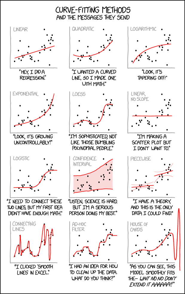
Why do I put this picture (see <a href=https://www.explainxkcd.com/wiki/index.php/2048:_Curve-Fitting>here</a> for explanation) right in front of everything? Have I caught your attention? Hopefully I have. These days, blogs on data science topic are dime a dozen. Some blogs teach you how to use decision tree/random forrest to predict the stock price movement, others illustrate the possibility of back-propagation neural network to forecast a bond price. The brutal truth is, most of them are nothing but house of cards. So far, I have not heard any quant shops hit the jackpot via machine learning. Most applications of machine learning in trading are leaned towards analytics rather than prediction or execution. One quant estimates the failure rate of machine learning in live tests of trading is at about <a href=https://www.bloomberg.com/news/articles/2019-07-11/why-machine-learning-hasn-t-made-investors-smarter-quicktake>90%</a>.
Monte Carlo, my first thought on these two words is the grand casino, where you dress up in tuxedo, meet Famke Janssen after car chase and introduce yourself in a deep sexy voice, 'Bond, James Bond'. Indeed, the simulation is named after the infamous casino in Monaco near Côte d'Azur. It actually refers to the computer simulation of massive amount of random events. This unconventional mathematical method is extremely powerful in the study of stochastic process. Here comes the argument on Linkedin that caught my eyes the other day. "Stock price can be seemed as a <a href=https://en.wikipedia.org/wiki/Wiener_process>Wiener Process</a>. Hence, we can use Monte Carlo simulation to predict the stock price." said a data science blog. Well, in order to be a Wiener Process, we have to assume the stock price is continuous in time. In reality, the market closes. The overnight volatility exists. But that is not the biggest issue here. The biggest issue is, can we really use Monte Carlo simulation to predict the stock price, even a range or its direction?
The author offered a quite interesting idea. As he suggested, the first step was to run as many simulations as possible on <a href=https://en.wikipedia.org/wiki/Stochastic_differential_equation#Use_in_probability_and_mathematical_finance>stochastic differential equations</a> to predict stock price. The goal of simulations was to pick a best fitted curve (in translation, the smallest standard deviation) compared to the historical data. There might exist a hidden pattern in the historical log return. The best fitted curve had the potential to replicate the hidden pattern and reflect it in the future forecast. The idea sounds neat, doesn't it? Inspired by his idea, we can build up the simulation accordingly. To fully unlock the potential of Monte Carlo simulation on fat tail events, the ticker we pick is General Electric, one of the worst performing stock in 2018. The share price of GE plunged 57.9% in 2018 thanks to its long history of M&A failures. The time horizon of the data series is 2016/1/15-2019/1/15. We split the series into halves, the first half as training horizon and the second half as testing horizon. Monte Carlo simulation will only justify its power if it can predict an extreme event like this.
Let's take a look at the figure below. Wow, what a great fit! The best fit is almost like running a cool linear regression with valid input. As you can see, it smoothly fits the curve in training horizon.
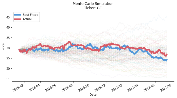
If we extend it to testing horizon...
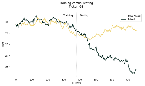
Oops, house of cards collapses. The real momentum is completely the opposite to the forecast, let alone the actual price. The forecast looks quite okay for the first 50 days of testing horizon. After that, the real momentum falls like a stone down through the deep sea while the forecast is gently climbing up. You may argue the number of the iterations is too small so we cannot make a case. Not exactly, let's look at the figure below.
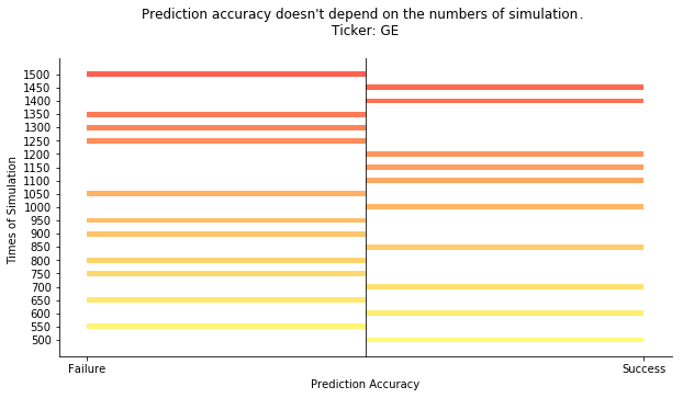
We start from 500 times of simulation to 1500 times of simulation. Each round we increase the number by 50. We don't look at the actual price forecast, just the direction. If the end price of testing horizon is larger than the end price of training horizon, we define it as gain. Vice versa. Only when both actual and forecast directions align, we consider the forecast is accurate. As the result shows, the prediction accuracy is irrelavant to the numbers of simulation. The accuracy is more sort of tossing a coin to guess heads or tails regardless of the times of simulation. If you think 1500 is still not large enough, you can definitely try 150000, be my guest. We don't have so much computing power as an individual user (frankly no patience is the real reason) but I can assure you the result is gonna stay the same. <a href=https://en.wikipedia.org/wiki/Law_of_large_numbers>Law of Large Numbers</a> theorem would not work here.
Now that the prophet of Monte Carlo turns out to be a con artist. Does Monte Carlo simulation have any application in risk management? Unless you are drinking the Kool-Aid. Let's extend the first figure a little bit longer to the end of testing horizon.
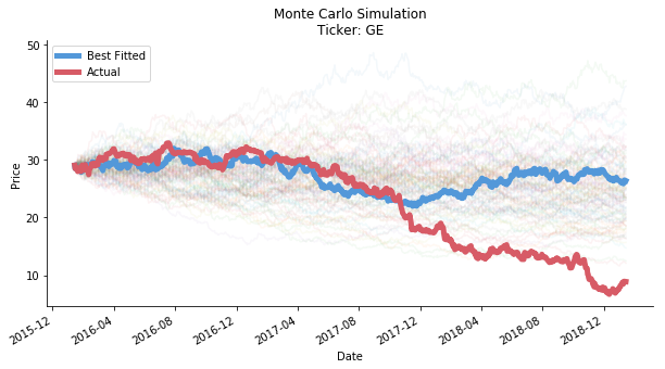
Obviously, out of 500 times of simulation, none of them successfully predict the scale of the downslide. The lowest price of 500 predictions is 10.99 per share. It is still way higher than the real bottom price at 6.71 per share (no wonder GE got its ass kicked out of DJIA). The so-called fat tail event simulation is merely a mirage. If you think GE in 2018 is an extreme case, you'd be so wrong. The next ticker we test is Nvidia from 2006/1/15 to 2009/1/15. In 2008, the share price of Nvidia dropped 75.6%!! The financial crisis is the true playground for risk quants. By default, we continue to split the time horizon of NVDA into two parts by 50:50. The result is in the figure below.
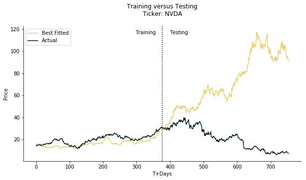
Undoubtedly, the best forecast fails the expectation again. It cannot accurately predict the direction of the momentum. For the extreme event, Monte Carlo simulation cannot predict the scale of downslide, again! 6.086 per share is the lowest price we achieve from our 500 times of simulation, yet the actual lowest is at 5.9 per share.
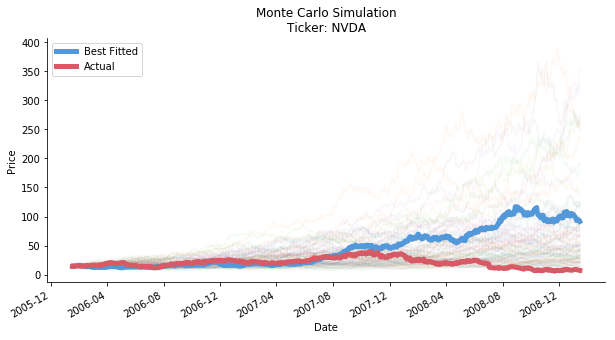
Still thinking about Monte Carlo for your next big project?
================================================
FILE: Oil Money project/Oil Money CAD.py
================================================
# coding: utf-8
# In[1]:
import pandas as pd
import os
import matplotlib.pyplot as plt
import copy
import matplotlib.patches as mpatches
from mpl_toolkits import mplot3d
import matplotlib.cm as cm
import statsmodels.api as sm
import numpy as np
from sklearn.cluster import KMeans
from sklearn.metrics import silhouette_score,silhouette_samples
from sklearn.model_selection import train_test_split
os.chdir('d:/')
# In[2]:
#plot two curves on same x axis, different y axis
def dual_axis_plot(xaxis,data1,data2,fst_color='r',
sec_color='b',fig_size=(10,5),
x_label='',y_label1='',y_label2='',
legend1='',legend2='',grid=False,title=''):
fig=plt.figure(figsize=fig_size)
ax=fig.add_subplot(111)
ax.set_xlabel(x_label)
ax.set_ylabel(y_label1, color=fst_color)
ax.plot(xaxis, data1, color=fst_color,label=legend1)
ax.tick_params(axis='y',labelcolor=fst_color)
ax.yaxis.labelpad=15
plt.legend(loc=3)
ax2=ax.twinx()
ax2.set_ylabel(y_label2, color=sec_color,rotation=270)
ax2.plot(xaxis, data2, color=sec_color,label=legend2)
ax2.tick_params(axis='y',labelcolor=sec_color)
ax2.yaxis.labelpad=15
fig.tight_layout()
plt.legend(loc=4)
plt.grid(grid)
plt.title(title)
plt.show()
#get distance between a point and a line
def get_distance(x,y,a,b):
temp1=y-x*a-b
temp2=(a**2+1)**0.5
return np.abs(temp1/temp2)
#create line equation from two points
def get_line_params(x1,y1,x2,y2):
a=(y1-y2)/(x1-x2)
b=y1-a*x1
return a,b
# In[3]:
df=pd.read_csv('wcs crude cadaud.csv',encoding='utf-8')
df.set_index('date',inplace=True)
# In[4]:
df.index=pd.to_datetime(df.index,format='%m/%d/%Y')
# In[5]:
df=df.reindex(columns=
['cny',
'gbp',
'usd',
'eur',
'krw',
'mxn',
'gas',
'wcs',
'edmonton',
'wti',
'gold',
'jpy',
'cad'])
# In[6]:
#create r squared bar charts
var=locals()
for i in df.columns:
if i!='cad':
x=sm.add_constant(df[i])
y=df['cad']
m=sm.OLS(y,x).fit()
var[str(i)]=m.rsquared
ax=plt.figure(figsize=(10,5)).add_subplot(111)
ax.spines['top'].set_visible(False)
ax.spines['right'].set_visible(False)
width=0.7
colorlist=['#9499a6','#9499a6','#9499a6','#9499a6',
'#9499a6','#9499a6','#9499a6','#582a20',
'#be7052','#f2c083','#9499a6','#9499a6']
temp=list(df.columns)
for i in temp:
if i!='cad':
plt.bar(temp.index(i)+width,
var[str(i)],width=width,label=i,
color=colorlist[temp.index(i)])
plt.title('Regressions on Loonie')
plt.ylabel('R Squared\n')
plt.xlabel('\nRegressors')
plt.xticks(np.arange(len(temp))+width,
['Yuan', 'Sterling', 'Dollar', 'Euro', 'KRW',
'MXN', 'Gas', 'WCS', 'Edmonton',
'WTI', 'Gold', 'Yen'],fontsize=10)
plt.show()
# In[7]:
#normalized value of loonie,yuan and sterling
ax=plt.figure(figsize=(10,5)).add_subplot(111)
ax.spines['top'].set_visible(False)
ax.spines['right'].set_visible(False)
(df['cny']/df['cny'].iloc[0]).plot(c='#77c9d4',label='Yuan')
(df['gbp']/df['gbp'].iloc[0]).plot(c='#57bc90',label='Sterling')
(df['cad']/df['cad'].iloc[0]).plot(c='#015249',label='Loonie')
plt.legend(loc=0)
plt.xlabel('Date')
plt.ylabel('Normalized Value by 100')
plt.title('Loonie vs Yuan vs Sterling')
plt.show()
# In[8]:
#normalized value of wti,wcs and edmonton
ax=plt.figure(figsize=(10,5)).add_subplot(111)
ax.spines['top'].set_visible(False)
ax.spines['right'].set_visible(False)
(df['wti']/df['wti'].iloc[0]).plot(c='#2a78b2',
label='WTI',alpha=0.5)
(df['wcs']/df['wcs'].iloc[0]).plot(c='#7b68ee',
label='WCS',alpha=0.5)
(df['edmonton']/df['edmonton'].iloc[0]).plot(c='#110b3c',
label='Edmonton',alpha=0.5)
plt.legend(loc=0)
plt.xlabel('Date')
plt.ylabel('Normalized Value by 100')
plt.title('Crude Oil Blends')
plt.show()
# In[9]:
dual_axis_plot(df.index,df['cad'],df['wcs'],
x_label='Date',y_label1='Canadian Dollar',
y_label2='Western Canadian Select',
legend1='Loonie',
legend2='WCS',
title='Loonie VS WCS in AUD',
fst_color='#a5a77f',sec_color='#d8dc2c')
dual_axis_plot(df.index,
np.divide(df['cad'],df['usd']),
np.divide(df['wcs'],df['usd']),
x_label='Date',y_label1='Canadian Dollar',
y_label2='Western Canadian Select',
legend1='Loonie',
legend2='WCS',
title='Loonie VS WCS in USD',
fst_color='#eb712f',sec_color='#91371b')
# In[10]:
#using elbow method to find optimal number of clusters
df['date']=[i for i in range(len(df.index))]
x=df[['cad','wcs','date']].reset_index(drop=True)
sse=[]
for i in range(1, 8):
kmeans = KMeans(n_clusters = i)
kmeans.fit(x)
sse.append(kmeans.inertia_/10000)
a,b=get_line_params(0,sse[0],len(sse)-1,sse[-1])
distance=[]
for i in range(len(sse)):
distance.append(get_distance(i,sse[i],a,b))
dual_axis_plot(np.arange(1,len(distance)+1),sse,distance,
x_label='Numbers of Cluster',y_label1='Sum of Squared Error',
y_label2='Perpendicular Distance',legend1='SSE',legend2='Distance',
title='Elbow Method for K Means',fst_color='#116466',sec_color='#e85a4f')
# In[11]:
#using silhouette score to find optimal number of clusters
sil=[]
for n in range(2,8):
clf=KMeans(n).fit(x)
projection=clf.predict(x)
sil.append(silhouette_score(x,projection))
ax=plt.figure(figsize=(10,5)).add_subplot(111)
ax.spines['top'].set_visible(False)
ax.spines['right'].set_visible(False)
ax.plot(np.arange(2,len(sil)+2),sil,
label='Silhouette',c='#5c0811',
drawstyle='steps-mid')
ax.plot(sil.index(max(sil))+2,max(sil),
marker='*',markersize=20,lw=0,
label='Max Score',c='#d94330')
plt.ylabel('Silhouette Score')
plt.xlabel('Numbers of Cluster')
plt.title('Silhouette Analysis for K Means')
plt.legend(loc=0)
plt.show()
# In[12]:
#k means
clf=KMeans(n_clusters=2).fit(x)
df['class']=clf.predict(x)
threshold=df[df['class']==0].index[-1]
# In[13]:
#plot clusters in 3d figure
ax=plt.figure(figsize=(10,7)).add_subplot(111, projection='3d')
xdata=df['wcs']
ydata=df['cad']
zdata=df['date']
ax.scatter3D(xdata[df['class']==0],ydata[df['class']==0],
zdata[df['class']==0],c='#faed26',s=10,alpha=0.5,
label='Before {}'.format(threshold.strftime('%Y-%m-%d')))
ax.scatter3D(xdata[df['class']==1],ydata[df['class']==1],
zdata[df['class']==1],c='#46344e',s=10,alpha=0.5,
label='After {}'.format(threshold.strftime('%Y-%m-%d')))
ax.grid(False)
for i in ax.w_xaxis, ax.w_yaxis, ax.w_zaxis:
i.pane.set_visible(False)
ax.set_xlabel('WCS')
ax.set_ylabel('Loonie')
ax.set_zlabel('Date')
ax.set_title('K Means on Loonie')
ax.legend(loc=6,bbox_to_anchor=(0.12, -0.1), ncol=4)
plt.show()
#to generate gif, u can use the following code
#it generates 3d figures from different angles
#use imageio to concatenate
"""
for ii in range(0,360,10):
ax.view_init(elev=10., azim=ii)
plt.savefig("cad kmeans%d.png" % (ii))
import imageio
filenames=["movie%d.png" % (ii) for ii in range(0,360,10)]
images=list(map(lambda filename:imageio.imread(filename),
filenames))
imageio.mimsave('cad kmeans.gif',images,duration = 0.2)
"""
# In[14]:
#create before/after regression comparison
#the threshold is based upon the finding of k means
m=sm.OLS(df['cad'][df['class']==0],sm.add_constant(df['wcs'][df['class']==0])).fit()
before=m.rsquared
m=sm.OLS(df['cad'][df['class']==1],sm.add_constant(df['wcs'][df['class']==1])).fit()
after=m.rsquared
ax=plt.figure(figsize=(10,5)).add_subplot(111)
ax.spines['top'].set_visible(False)
ax.spines['right'].set_visible(False)
plt.bar(['Before {}'.format(threshold.strftime('%Y-%m-%d')),
'After {}'.format(threshold.strftime('%Y-%m-%d'))],
[before,after],color=['#f172a1','#a1c3d1'])
plt.ylabel('R Squared')
plt.title('Cluster + Regression')
plt.show()
# In[15]:
#create 1 std, 2 std band
for i in range(2):
x_train,x_test,y_train,y_test=train_test_split(
sm.add_constant(df['wcs'][df['class']==i]),
df['cad'][df['class']==i],test_size=0.5,shuffle=False)
m=sm.OLS(y_test,x_test).fit()
forecast=m.predict(x_test)
ax=plt.figure(figsize=(10,5)).add_subplot(111)
ax.spines['top'].set_visible(False)
ax.spines['right'].set_visible(False)
forecast.plot(label='Fitted',c='#ab987a')
y_test.plot(label='Actual',c='#ff533d')
ax.fill_between(y_test.index,
forecast+np.std(m.resid),
forecast-np.std(m.resid),
color='#0f1626', \
alpha=0.6, \
label='1 Sigma')
ax.fill_between(y_test.index,
forecast+2*np.std(m.resid),
forecast-2*np.std(m.resid),
color='#0f1626', \
alpha=0.8, \
label='2 Sigma')
plt.legend(loc=0)
title='Before '+threshold.strftime('%Y-%m-%d') if i==0 else 'After '+threshold.strftime('%Y-%m-%d')
plt.title(f'{title}\nCanadian Dollar Positions\nR Squared {round(m.rsquared*100,2)}%\n')
plt.xlabel('\nDate')
plt.ylabel('CADAUD')
plt.show()
================================================
FILE: Oil Money project/Oil Money COP.py
================================================
# coding: utf-8
# In[1]:
import pandas as pd
import os
import matplotlib.pyplot as plt
import statsmodels.api as sm
import seaborn as sns
import numpy as np
from sklearn.model_selection import train_test_split
os.chdir('k:/')
# In[2]:
#plot two curves on same x axis, different y axis
def dual_axis_plot(xaxis,data1,data2,fst_color='r',
sec_color='b',fig_size=(10,5),
x_label='',y_label1='',y_label2='',
legend1='',legend2='',grid=False,title=''):
fig=plt.figure(figsize=fig_size)
ax=fig.add_subplot(111)
ax.set_xlabel(x_label)
ax.set_ylabel(y_label1, color=fst_color)
ax.plot(xaxis, data1, color=fst_color,label=legend1)
ax.tick_params(axis='y',labelcolor=fst_color)
ax.yaxis.labelpad=15
plt.legend(loc=3)
ax2=ax.twinx()
ax2.set_ylabel(y_label2, color=sec_color,rotation=270)
ax2.plot(xaxis, data2, color=sec_color,label=legend2)
ax2.tick_params(axis='y',labelcolor=sec_color)
ax2.yaxis.labelpad=15
fig.tight_layout()
plt.legend(loc=4)
plt.grid(grid)
plt.title(title)
plt.show()
# In[3]:
#read dataframe
df=pd.read_csv('vas crude copaud.csv',encoding='utf-8')
df.set_index('date',inplace=True)
df.index=pd.to_datetime(df.index)
# In[4]:
#run regression on each input
D={}
for i in df.columns:
if i!='cop':
x=sm.add_constant(df[i])
y=df['cop']
m=sm.OLS(y,x).fit()
D[i]=m.rsquared
D=dict(sorted(D.items(),key=lambda x:x[1],reverse=True))
# In[5]:
#create r squared bar charts
colorlist=[]
for i in D:
if i =='wti':
colorlist.append('#447294')
elif i=='brent':
colorlist.append('#8fbcdb')
elif i=='vasconia':
colorlist.append('#f4d6bc')
else:
colorlist.append('#cdc8c8')
ax=plt.figure(figsize=(10,5)).add_subplot(111)
ax.spines['top'].set_visible(False)
ax.spines['right'].set_visible(False)
width=0.7
for i in D:
plt.bar(list(D.keys()).index(i)+width,
D[i],width=width,label=i,
color=colorlist[list(D.keys()).index(i)])
plt.title('Regressions on COP')
plt.ylabel('R Squared\n')
plt.xlabel('\nRegressors')
plt.xticks(np.arange(len(D))+width,
[i.upper() for i in D.keys()],fontsize=8)
plt.show()
# In[6]:
#normalized value of wti,brent and vasconia
ax=plt.figure(figsize=(10,5)).add_subplot(111)
ax.spines['top'].set_visible(False)
ax.spines['right'].set_visible(False)
(df['vasconia']/df['vasconia'].iloc[0]).plot(c='#6f6ff4',
label='Vasconia',alpha=0.5)
(df['brent']/df['brent'].iloc[0]).plot(c='#e264c0',
label='Brent',alpha=0.5)
(df['wti']/df['wti'].iloc[0]).plot(c='#fb6630',
label='WTI',alpha=0.5)
plt.legend(loc=0)
plt.xlabel('Date')
plt.ylabel('Normalized Value by 100')
plt.title('Crude Oil Blends')
plt.show()
# In[7]:
#cop vs gold
dual_axis_plot(df.index,df['cop'],df['gold'],
x_label='Date',y_label1='Colombian Peso',
y_label2='Gold LBMA',
legend1='COP',
legend2='Gold',
title='COP VS Gold',
fst_color='#96CEB4',sec_color='#FFA633')
#cop vs usd
dual_axis_plot(df.index,df['cop'],df['usd'],
x_label='Date',y_label1='Colombian Peso',
y_label2='US Dollar',
legend1='COP',
legend2='USD',
title='COP VS USD',
fst_color='#9DE0AD',sec_color='#5C4E5F')
# In[8]:
#cop vs brl
dual_axis_plot(df.index,df['cop'],df['brl'],
x_label='Date',y_label1='Colombian Peso',
y_label2='Brazilian Real',
legend1='COP',
legend2='BRL',
title='COP VS BRL',
fst_color='#a4c100',sec_color='#f7db4f')
#usd vs mxn
dual_axis_plot(df.index,df['usd'],df['mxn'],
x_label='Date',y_label1='US Dollar',
y_label2='Mexican Peso',
legend1='USD',
legend2='MXN',
title='USD VS MXN',
fst_color='#F4A688',sec_color='#A2836E')
#cop vs mxn
dual_axis_plot(df.index,df['cop'],df['mxn'],
x_label='Date',y_label1='Colombian Peso',
y_label2='Mexican Peso',
legend1='COP',
legend2='MXN',
title='COP VS MXN',
fst_color='#F26B38',sec_color='#B2AD7F')
# In[9]:
#cop vs vasconia
dual_axis_plot(df.index,df['cop'],df['vasconia'],
x_label='Date',y_label1='Colombian Peso',
y_label2='Vasconia Crude',
legend1='COP',
legend2='Vasconia',
title='COP VS Vasconia',
fst_color='#346830',sec_color='#BBAB9B')
# In[10]:
#create before/after regression comparison
m=sm.OLS(df['cop'][:'2016'],sm.add_constant(df['vasconia'][:'2016'])).fit()
before=m.rsquared
m=sm.OLS(df['cop']['2017':],sm.add_constant(df['vasconia']['2017':])).fit()
after=m.rsquared
ax=plt.figure(figsize=(10,5)).add_subplot(111)
ax.spines['top'].set_visible(False)
ax.spines['right'].set_visible(False)
plt.bar(['Before 2017',
'After 2017'],
[before,after],color=['#82b74b', '#5DD39E'])
plt.ylabel('R Squared')
plt.title('Before/After Regression')
plt.show()
# In[11]:
#create 1 std, 2 std band before 2017
x_train,x_test,y_train,y_test=train_test_split(
sm.add_constant(df['vasconia'][:'2016']),
df['cop'][:'2016'],test_size=0.5,shuffle=False)
m=sm.OLS(y_test,x_test).fit()
forecast=m.predict(x_test)
ax=plt.figure(figsize=(10,5)).add_subplot(111)
ax.spines['top'].set_visible(False)
ax.spines['right'].set_visible(False)
forecast.plot(label='Fitted',c='#FEFBD8')
y_test.plot(label='Actual',c='#ffd604')
ax.fill_between(y_test.index,
forecast+np.std(m.resid),
forecast-np.std(m.resid),
color='#F4A688',
alpha=0.6,
label='1 Sigma')
ax.fill_between(y_test.index,
forecast+2*np.std(m.resid),
forecast-2*np.std(m.resid),
color='#8c7544',
alpha=0.8,
label='2 Sigma')
plt.legend(loc=0)
plt.title(f'Colombian Peso Positions\nR Squared {round(m.rsquared*100,2)}%\n')
plt.xlabel('\nDate')
plt.ylabel('COPAUD')
plt.show()
# In[12]:
#create 1 std, 2 std band after 2017
x_train,x_test,y_train,y_test=train_test_split(
sm.add_constant(df['vasconia']['2017':]),
df['cop']['2017':],test_size=0.5,shuffle=False)
m=sm.OLS(y_test,x_test).fit()
forecast=m.predict(x_test)
ax=plt.figure(figsize=(10,5)).add_subplot(111)
ax.spines['top'].set_visible(False)
ax.spines['right'].set_visible(False)
forecast.plot(label='Fitted',c='#FEFBD8')
y_test.plot(label='Actual',c='#ffd604')
ax.fill_between(y_test.index,
forecast+np.std(m.resid),
forecast-np.std(m.resid),
color='#F4A688',
alpha=0.6,
label='1 Sigma')
ax.fill_between(y_test.index,
forecast+2*np.std(m.resid),
forecast-2*np.std(m.resid),
color='#8c7544', \
alpha=0.8, \
label='2 Sigma')
plt.legend(loc=0)
plt.title(f'Colombian Peso Positions\nR Squared {round(m.rsquared*100,2)}%\n')
plt.xlabel('\nDate')
plt.ylabel('COPAUD')
plt.show()
# In[13]:
#shrink data size for better viz
dataset=df['2016':]
dataset.reset_index(inplace=True)
# In[14]:
#import the strategy script as this is a script for analytics and visualization
#the official trading strategy script is in the following link
# https://github.com/je-suis-tm/quant-trading/blob/master/Oil%20Money%20project/Oil%20Money%20Trading%20backtest.py
import oil_money_trading_backtest as om
#generate signals,monitor portfolio performance
#plot positions and total asset
signals=om.signal_generation(dataset,'vasconia','cop',om.oil_money,stop=0.001)
p=om.portfolio(signals,'cop')
om.plot(signals,'cop')
om.profit(p,'cop')
# In[15]:
#try different holding period and stop loss/profit point
dic={}
for holdingt in range(5,20):
for stopp in np.arange(0.001,0.005,0.0005):
signals=om.signal_generation(dataset,'vasconia','cop',om.oil_money,
holding_threshold=holdingt,
stop=round(stopp,4))
p=om.portfolio(signals,'cop')
dic[holdingt,round(stopp,4)]=p['asset'].iloc[-1]/p['asset'].iloc[0]-1
profile=pd.DataFrame({'params':list(dic.keys()),'return':list(dic.values())})
# In[16]:
#plotting the distribution of return
ax=plt.figure(figsize=(10,5)).add_subplot(111)
ax.spines['top'].set_visible(False)
ax.spines['right'].set_visible(False)
profile['return'].apply(lambda x:x*100).hist(histtype='bar',
color='#b2660e',
width=0.45,bins=20)
plt.title('Distribution of Return on COP Trading')
plt.grid(False)
plt.ylabel('Frequency')
plt.xlabel('Return (%)')
plt.show()
# In[17]:
#plotting the heatmap of return under different parameters
#try to find the optimal parameters to maximize the return
#convert the dataframe into a matrix format first
matrix=pd.DataFrame(columns=[round(i,4) for i in np.arange(0.001,0.005,0.0005)])
matrix['index']=np.arange(5,20)
matrix.set_index('index',inplace=True)
for i,j in profile['params']:
matrix.at[i,round(j,4)]= profile['return'][profile['params']==(i,j)].item()*100
for i in matrix.columns:
matrix[i]=matrix[i].apply(float)
#plotting
fig=plt.figure(figsize=(10,5))
ax=fig.add_subplot(111)
sns.heatmap(matrix,cmap=plt.cm.viridis,
xticklabels=3,yticklabels=3)
ax.collections[0].colorbar.set_label('Return(%)\n',
rotation=270)
plt.xlabel('\nStop Loss/Profit (points)')
plt.ylabel('Position Holding Period (days)\n')
plt.title('Profit Heatmap\n',fontsize=10)
plt.style.use('default')
#it seems like the return doesnt depend on the stop profit/loss point
#it is correlated with the length of holding period
#the ideal one should be 17 trading days
#as for stop loss/profit point could range from 0.002 to 0.005
================================================
FILE: Oil Money project/Oil Money NOK.py
================================================
# coding: utf-8
# In[1]:
#i call it oil money
#cuz its a statistical arbitrage on crude benchmark and petrocurrency
#the inspiration came from an article i read
#it suggested to trade on petrocurrency when the oil price went uprising
#plus overall volatility for forex market was low
#the first thing is to build up a model to explore the causality
#we split the historical datasets into two parts
#one for the model estimation, the other for the model validation
#we do a regression on estimation horizon
#we use linear regression to make a prediction on ideal price level
#we set up thresholds based on the standard deviation of residual
#take one deviation above as the upper threshold
#if the currency price breaches the upper threshold
#take a short position as it is assumed to revert to its 'normal' price range soon
#vice versa
#so its kinda like bollinger bands
#however, our regression is based on statistics
#we still need to consider fundamental influence
#what if the market condition has changed
#in that case our model wont work any more
#well,all models lose their creditability over the time
#denote the price deviating two sigmas away from predicted value as model failure
#which we should revert our positions
#e.g. the price is two sigmas above our predicted value
#we change our short to long since the market has changed its sentiment
#there is probably hidden information in the uprising price
#lets follow the trend and see where it ends
#this idea sounds very silly
#nobody actually does it or not that i know of
#i just wanna to see if the idea would work
#perhaps the idea would bring a huge loss
#nonetheless, it turns out to be a big surprise!
#first, we choose our currency norwegian krone
#norway is one of the largest oil producing countries with floating fx regime
#other oil producing countries such as saudi, iran, venezuela have their fx pegged to usd
#russia is supposed to be a good training set
#nevertheless, russia gets sanctioned by uncle sam a lot
#we would see this in the next script
# https://github.com/je-suis-tm/quant-trading/blob/master/Oil%20Money%20project/Oil%20Money%20RUB.py
#after targetting at norwegian krone, we have to choose a currency to evaluate nok
#take a look at norway's biggest trading partners
#we should include us dollar, euro and uk sterling as well as brent crude price in our model
#in addition, the base currency would be japanese yen
#cuz its not a big trading partner with norway
#which implies it doesnt have much correlation with nok
#preparation is done, lets get started!
import matplotlib.pyplot as plt
import statsmodels.api as sm
import pandas as pd
import numpy as np
import seaborn as sns
from sklearn.linear_model import ElasticNetCV as en
from statsmodels.tsa.stattools import adfuller as adf
import os
os.chdir('d:/')
# In[2]:
df=pd.read_csv('brent crude nokjpy.csv')
df.set_index(pd.to_datetime(df[list(df.columns)[0]]),inplace=True)
del df[list(df.columns)[0]]
# In[3]:
#identification
#first of first, using scatter plot to visualize the correlation
#lets denote data from 2013-4-25 to 2017-4-25 as estimation horizon/training set
#lets denote data from 2017-4-25 to 2018-4-25 as validation horizon/testing set
ax=plt.figure(figsize=(10,5)).add_subplot(111)
ax.spines['top'].set_visible(False)
ax.spines['right'].set_visible(False)
ax.scatter(df['brent'][df.index<'2017-04-25'],df['nok'][df.index<'2017-04-25'],s=1,c='#5f0f4e')
plt.title('NOK Brent Correlation')
plt.xlabel('Brent in JPY')
plt.ylabel('NOKJPY')
plt.show()
#if we run a covariance matrix on nok and brent, we got
#np.corrcoef(df['nok'],df['brent'])
#array([[1. , 0.89681228],[0.89681228, 1. ]])
#dual axis plot
def dual_axis_plot(xaxis,data1,data2,fst_color='r',
sec_color='b',fig_size=(10,5),
x_label='',y_label1='',y_label2='',
legend1='',legend2='',grid=False,title=''):
fig=plt.figure(figsize=fig_size)
ax=fig.add_subplot(111)
ax.set_xlabel(x_label)
ax.set_ylabel(y_label1, color=fst_color)
ax.plot(xaxis, data1, color=fst_color,label=legend1)
ax.tick_params(axis='y',labelcolor=fst_color)
ax.yaxis.labelpad=15
plt.legend(loc=3)
ax2 = ax.twinx()
ax2.set_ylabel(y_label2, color=sec_color,rotation=270)
ax2.plot(xaxis, data2, color=sec_color,label=legend2)
ax2.tick_params(axis='y',labelcolor=sec_color)
ax2.yaxis.labelpad=15
fig.tight_layout()
plt.legend(loc=4)
plt.grid(grid)
plt.title(title)
plt.show()
#nok vs ir
dual_axis_plot(df.index,df['nok'],df['interest rate'],
fst_color='#34262b',sec_color='#cb2800',
fig_size=(10,5),x_label='Date',
y_label1='NOKJPY',y_label2='Norges Bank Interest Rate
%',
legend1='NOKJPY',legend2='Interest Rate',
grid=False,title='NOK vs Interest Rate')
#nok vs brent
dual_axis_plot(df.index,df['nok'],df['brent'],
fst_color='#4f2d20',sec_color='#3feee6',
fig_size=(10,5),x_label='Date',
y_label1='NOKJPY',y_label2='Brent in JPY',
legend1='NOKJPY',legend2='Brent',
grid=False,title='NOK vs Brent')
#nok vs gdp
#cuz gdp is released quarterly
#we need to convert nok into quarterly data as well
ind=df['gdp yoy'].dropna().index
dual_axis_plot(df.loc[ind].index,
df['nok'].loc[ind],
df['gdp yoy'].dropna(),
fst_color='#116466',sec_color='#ff652f',
fig_size=(10,5),x_label='Date',
y_label1='NOKJPY',y_label2='Norway GDP YoY %',
legend1='NOKJPY',legend2='GDP',
grid=False,title='NOK vs GDP')
#Now we do our linear regression
x0=pd.concat([df['usd'],df['gbp'],df['eur'],df['brent']],axis=1)
x1=sm.add_constant(x0)
x=x1[x1.index<'2017-04-25']
y=df['nok'][df.index<'2017-04-25']
model=sm.OLS(y,x).fit()
print(model.summary(),'\n')
# In[4]:
#from the summary u can tell there is multicollinearity
#the condition number is skyrocketing
#alternatively, i can use elastic net regression to achieve the convergence
#check the link below for more details
# https://github.com/je-suis-tm/machine-learning/blob/master/coordinate%20descent%20for%20elastic%20net.ipynb
m=en(alphas=[0.0001, 0.0005, 0.001, 0.01, 0.1, 1, 10],
l1_ratio=[.01, .1, .5, .9, .99], max_iter=5000).fit(x0[x0.index<'2017-04-25'], y)
print(m.intercept_,m.coef_)
#elastic net estimation results:
#3.79776228406 [ 0.00388958 0.01992038 0.02823187 0.00050092]
# In[5]:
#calculate the fitted value of nok
df['sk_fit']=(df['usd']*m.coef_[0]+df['gbp']*m.coef_[1]+
df['eur']*m.coef_[2]+df['brent']*m.coef_[3]+m.intercept_)
# In[6]:
#getting the residual
df['sk_residual']=df['nok']-df['sk_fit']
#one can always argue what if we eliminate some regressors
#in econometrics, if adding extra variables do not decrease adjusted r squared
#or worsen AIC, BIC
#we should include more information as long as it makes sense
# In[7]:
#lets generate signals based on the elastic net
#we set one sigma of the residual as thresholds
#two sigmas of the residual as stop orders
#which is common practise in statistics
upper=np.std(df['sk_residual'][df.index<'2017-04-25'])
lower=-upper
signals=pd.concat([df[i] for i in ['nok', 'usd', 'eur', 'gbp', 'brent', 'sk_fit','sk_residual']], \
axis=1)[df.index>='2017-04-25']
signals['fitted']=signals['sk_fit']
del signals['sk_fit']
signals['upper']=signals['fitted']+upper
signals['lower']=signals['fitted']+lower
signals['stop profit']=signals['fitted']+2*upper
signals['stop loss']=signals['fitted']+2*lower
signals['signals']=0
# In[8]:
#while doing a traversal
#we apply the rules mentioned before
#if actual price goes beyond upper threshold
#we take a short and bet on its reversion process
#vice versa
#we use cumsum to make sure our signals only get generated
#for the first time condions are met
#when actual price hits the stop order boundary
#we revert our positions
#u may wonder whats next for breaking the boundary
#well, we stop the signal generation algorithm
#we need to recalibrate our model or use other trend following strategies
index=list(signals.columns).index('signals')
for j in range(len(signals)):
if signals['nok'].iloc[j]>signals['upper'].iloc[j]:
signals.iloc[j,index]=-1
if signals['nok'].iloc[j]<signals['lower'].iloc[j]:
signals.iloc[j,index]=1
signals['cumsum']=signals['signals'].cumsum()
if signals['cumsum'].iloc[j]>1 or signals['cumsum'].iloc[j]<-1:
signals.iloc[j,index]=0
if signals['nok'].iloc[j]>signals['stop profit'].iloc[j]:
signals['cumsum']=signals['signals'].cumsum()
signals.iloc[j,index]=-signals['cumsum'].iloc[j]+1
signals['cumsum']=signals['signals'].cumsum()
break
if signals['nok'].iloc[j]<signals['stop loss'].iloc[j]:
signals['cumsum']=signals['signals'].cumsum()
signals.iloc[j,index]=-signals['cumsum'].iloc[j]-1
signals['cumsum']=signals['signals'].cumsum()
break
# In[9]:
#next, we plot the usual positions as the first figure
ax=plt.figure(figsize=(10,5)).add_subplot(111)
ax.spines['top'].set_visible(False)
ax.spines['right'].set_visible(False)
signals['nok'].plot(label='NOKJPY',c='#594f4f',alpha=0.5)
ax.plot(signals.loc[signals['signals']>0].index,
signals['nok'][signals['signals']>0],
lw=0,marker='^',c='#83af9b',label='LONG', markersize=10)
ax.plot(signals.loc[signals['signals']<0].index,
signals['nok'][signals['signals']<0],
lw=0,marker='v',c='#fe4365',label='SHORT', markersize=10)
ax.plot(pd.to_datetime('2017-12-20'),
signals['nok'].loc['2017-12-20'],
lw=0,marker='*',c='#f9d423', markersize=15, alpha=0.8,
label='Potential Exit Point of Momentum Trading')
plt.axvline('2017/11/15',linestyle=':',c='k',label='Exit')
plt.legend()
plt.title('NOKJPY Positions')
plt.ylabel('NOKJPY')
plt.xlabel('Date')
plt.show()
# In[10]:
#the second figure explores thresholds and boundaries for signal generation
#we can see after 2017/11/15, nokjpy price went skyrocketing
#as a data scientist, we must ask why?
#is it a problem of our model identification
#or the fundamental situation of nokjpy or oil changed
ax=plt.figure(figsize=(10,5)).add_subplot(111)
ax.spines['top'].set_visible(False)
ax.spines['right'].set_visible(False)
signals['fitted'].plot(lw=2.5,label='Fitted',c='w',alpha=0.6)
signals['nok'].plot(lw=2,label='Actual',c='#04060f',alpha=0.8)
ax.fill_between(signals.index,signals['upper'],
signals['lower'],alpha=0.2,label='1 Sigma',color='#2a3457')
ax.fill_between(signals.index,signals['stop profit'],
signals['stop loss'],alpha=0.1,label='2 Sigma',color='#720017')
plt.legend(loc='best')
plt.title('Fitted vs Actual')
plt.ylabel('NOKJPY')
plt.xlabel('Date')
plt.show()
# In[11]:
#if we decompose nokjpy into long term trend and short term random process
#we could clearly see that brent crude price has dominated short term random process
#so what changed the long term trend?
#there are a few possible reasons
#saudi and iran endorsed an extension of production caps on that particular date
#donald trump got elected as potus so he would encourage a depreciated us dollar
#which ultimately pushed up the oil price
# In[12]:
#lets normalize all prices by 100
#its easy to see that nok follows euro
#and economics explanation would be norway is in eea
#its economy heavily relies on eu
ax=plt.figure(figsize=(10,5)).add_subplot(111)
ax.spines['top'].set_visible(False)
ax.spines['right'].set_visible(False)
(df['nok']/df['nok'][0]*100).plot(c='#ff8c94',label='Norwegian Krone',alpha=0.9)
(df['usd']/df['usd'][0]*100).plot(c='#9de0ad',label='US Dollar',alpha=0.9)
(df['eur']/df['eur'][0]*100).plot(c='#45ada8',label='Euro',alpha=0.9)
(df['gbp']/df['gbp'][0]*100).plot(c='#f8b195',label='UK Sterling',alpha=0.9)
(df['brent']/df['brent'][0]*100).plot(c='#6c5b7c',label='Brent Crude',alpha=0.5)
plt.legend(loc='best')
plt.ylabel('Normalized Price by 100')
plt.xlabel('Date')
plt.title('Trend')
plt.show()
# In[13]:
#that still doesnt sound convincable
#lets try cointegration test
#academically we should use johansen test which works on multi dimensions
#unfortunately, there is no johansen test in statsmodels (at the time i wrote this script)
#well, here we go again
#we have to use Engle-Granger two step!
#salute to Engle, mentor of my mentor Gallo
#to the nobel prize winner
#im not gonna explain much here
#if u have checked my other codes, u sould know
#details are in pair trading session
# https://github.com/je-suis-tm/quant-trading/blob/master/Pair%20trading%20backtest.py
x2=df['eur'][df.index<'2017-04-25']
x3=sm.add_constant(x2)
model=sm.OLS(y,x3).fit()
ero=model.resid
print(adf(ero))
print(model.summary())
#(-2.5593457642922992, 0.10169409761939013, 0, 1030,
#{'1%': -3.4367147300588341, '5%': -2.8643501440982058, '10%': -2.5682662399849185}, -1904.8360920752475)
#0.731199409071
#unfortunately, the residual hasnt even reached 90% confidence interval
#we cant conclude any cointegration from the test
#still, from the visualization
#we can tell nok and eur are somewhat correlated
#our rsquared suggested euro has the power of 73% explanation on nok
# In[14]:
#then lets do a pnl analysis
capital0=2000
positions=100
portfolio=pd.DataFrame(index=signals.index)
portfolio['holding']=signals['nok']*signals['cumsum']*positions
portfolio['cash']=capital0-(signals['nok']*signals['signals']*positions).cumsum()
portfolio['total asset']=portfolio['holding']+portfolio['cash']
portfolio['signals']=signals['signals']
# In[15]:
portfolio=portfolio[portfolio.index>'2017-10-01']
portfolio=portfolio[portfolio.index<'2018-01-01']
# In[16]:
#we plot how our asset value changes over time
ax=plt.figure(figsize=(10,5)).add_subplot(111)
ax.spines['top'].set_visible(False)
ax.spines['right'].set_visible(False)
portfolio['total asset'].plot(c='#594f4f',alpha=0.5,label='Total Asset')
ax.plot(portfolio.loc[portfolio['signals']>0].index,portfolio['total asset'][portfolio['signals']>0],
lw=0,marker='^',c='#2a3457',label='LONG',markersize=10,alpha=0.5)
ax.plot(portfolio.loc[portfolio['signals']<0].index,portfolio['total asset'][portfolio['signals']<0],
lw=0,marker='v',c='#720017',label='The Big Short',markersize=15,alpha=0.5)
ax.fill_between(portfolio['2017-11-20':'2017-12-20'].index,
(portfolio['total asset']+np.std(portfolio['total asset']))['2017-11-20':'2017-12-20'],
(portfolio['total asset']-np.std(portfolio['total asset']))['2017-11-20':'2017-12-20'],
alpha=0.2, color='#547980')
plt.text(pd.to_datetime('2017-12-20'),
(portfolio['total asset']+np.std(portfolio['total asset'])).loc['2017-12-20'],
'What if we use MACD here?')
plt.axvline('2017/11/15',linestyle=':',label='Exit',c='#ff847c')
plt.legend()
plt.title('Portfolio Performance')
plt.ylabel('Asset Value')
plt.xlabel('Date')
plt.show()
#surprising when our model is valid for prediction
#its difficult to make money from thresholds oscillating
#when actual price goes beyond stop order boundary
#that is basically the most profitable trade ever
#best to follow up with a momentum strategy
#maybe this is not a statistical arbitrage after all
#the model is a trend following entry indicator
# In[17]:
#now lets construct a trend following strategy based on the previous strategy
#call it oil money version 2 or whatever
#here i would only import the strategy script as this is a script for analytics and visualization
#the official trading strategy script is in the following link
# https://github.com/je-suis-tm/quant-trading/blob/master/Oil%20Money%20project/Oil%20Money%20Trading%20backtest.py
import oil_money_trading_backtest as om
#generate signals,monitor portfolio performance
#plot positions and total asset
signals=om.signal_generation(dataset,'brent','nok',om.oil_money)
p=om.portfolio(signals,'nok')
om.plot(signals,'nok')
om.profit(p,'nok')
#but thats not enough, we are not happy with the return
#come on, 2 percent return?
#i may as well as deposit the money into the current account
#and get 0.75% risk free interest rate
#therefore, we gotta try different holding period and stop loss/profit point
#the double loop is very slow, i almost wanna do it in julia
#plz go get a coffee or even lunch and dont wait for it
dic={}
for holdingt in range(5,20):
for stopp in np.arange(0.3,1.1,0.05):
signals=om.signal_generation(dataset,'brent','nok',om.oil_money \
holding_threshold=holdingt, \
stop=stopp)
p=om.portfolio(signals,'nok')
dic[holdingt,stopp]=p['asset'].iloc[-1]/p['asset'].iloc[0]-1
profile=pd.DataFrame({'params':list(dic.keys()),'return':list(dic.values())})
# In[18]:
#plotting the distribution of return
#in average the return is 2%
#but we can get -6% and 6% as extreme values
#we dont give a crap about average
#we want the largest positive return
ax=plt.figure(figsize=(10,5)).add_subplot(111)
ax.spines['top'].set_visible(False)
ax.spines['right'].set_visible(False)
profile['return'].apply(lambda x:x*100).hist(histtype='bar', \
color='#f09e8c', \
width=0.45,bins=20)
plt.title('Distribution of Return on NOK Trading')
plt.grid(False)
plt.ylabel('Frequency')
plt.xlabel('Return (%)')
plt.show()
# In[19]:
#plotting the heatmap of return under different parameters
#try to find the optimal parameters to maximize the return
#turn the dataframe into a matrix format first
matrix=pd.DataFrame(columns= \
[round(i,2) for i in np.arange(0.3,1.1,0.05)])
matrix['index']=np.arange(5,20)
matrix.set_index('index',inplace=True)
for i,j in profile['params']:
matrix.at[i,round(j,2)]= \
profile['return'][profile['params']==(i,j)].item()*100
for i in matrix.columns:
matrix[i]=matrix[i].apply(float)
#plotting
fig=plt.figure(figsize=(10,5))
ax=fig.add_subplot(111)
sns.heatmap(matrix,cmap='gist_heat_r',square=True, \
xticklabels=3,yticklabels=3)
ax.collections[0].colorbar.set_label('Return(%) \n', \
rotation=270)
plt.xlabel('\nStop Loss/Profit (points)')
plt.ylabel('Position Holding Period (days)\n')
plt.title('Profit Heatmap\n',fontsize=10)
plt.style.use('default')
#it seems like the return doesnt depend on the stop profit/loss point
#it is correlated with the length of holding period
#the ideal one should be 9 trading days
#as for stop loss/profit point could range from 0.6 to 1.05
================================================
FILE: Oil Money project/Oil Money RUB.py
================================================
# coding: utf-8
# In[1]:
import os
import pandas as pd
import numpy as np
import statsmodels.api as sm
import matplotlib.pyplot as plt
import re
os.chdir('d:/')
df=pd.read_csv('urals crude rubaud.csv')
# In[2]:
df.set_index('date',inplace=True)
df.index=pd.to_datetime(df.index)
df.dropna(inplace=True)
# In[3]:
#this is the part to create r squared of different regressors
#in different years for stepwise regression
#we can use locals to create lists for different currency
#each list contains r squared of different years
year=df.index.year.drop_duplicates().tolist()
var=locals()
for i in df.columns:
if i!='rub':
var[i]=[]
for j in year:
x=sm.add_constant(df[i][str(j):str(j)])
y=df['rub'][str(j):str(j)]
m=sm.OLS(y,x).fit()
var[i].append(m.rsquared)
ax=plt.figure(figsize=(10,5)).add_subplot(111)
ax.spines['top'].set_visible(False)
ax.spines['right'].set_visible(False)
#to save you from the hassle
#just use these codes to generate the bar chart
width=0.3
colorlist=['#c0334d','#d6618f','#f3d4a0','#f1931b']
bar=locals()
for j in range(len(year)):
bar[j]=[var[i][j] for i in df.columns if i!='rub']
plt.bar(np.arange(1,len([i for i in df.columns if i!='rub'])*2+1,2)+j*width,
bar[j],width=width,label=year[j],color=colorlist[j])
plt.legend(loc=0)
plt.title('Stepwise Regression Year by Year')
plt.ylabel('R Squared')
plt.xlabel('Regressors')
plt.xticks(np.arange(1,len([i for i in df.columns if i!='rub'])*2+1,2)+(len(year)-1)*width/2,
['Urals Crude', 'Japanese\nYen',
'Euro', 'Henry Hub', 'Chinese\nYuan',
'Korean\nWon', 'Ukrainian\nHryvnia'],fontsize=10)
plt.show()
# In[4]:
#this is similar to In[3]
#In[3] is r squared of each regressor in each year
#In[4] is r squared of each regressor of years cumulated
var=locals()
for i in df.columns:
if i!='rub':
var[i]=[]
for j in year:
x=sm.add_constant(df[i][:str(j)])
y=df['rub'][:str(j)]
m=sm.OLS(y,x).fit()
var[i].append(m.rsquared)
ax=plt.figure(figsize=(10,5)).add_subplot(111)
ax.spines['top'].set_visible(False)
ax.spines['right'].set_visible(False)
width=0.3
colorlist=['#04060f','#03353e','#0294a5','#a79c93']
bar=locals()
for j in range(len(year)):
bar[j]=[var[i][j] for i in df.columns if i!='rub']
plt.bar(np.arange(1,len([i for i in df.columns if i!='rub'])*2+1,2)+j*width,
bar[j],width=width,label=year[j],color=colorlist[j])
plt.legend(loc=0)
plt.title('Stepwise Regression Year Cumulated')
plt.ylabel('R Squared')
plt.xlabel('Regressors')
plt.xticks(np.arange(1,len([i for i in df.columns if i!='rub'])*2+1,2)+(len(year)-1)*width/2,
['Urals Crude', 'Japanese\nYen',
'Euro', 'Henry Hub', 'Chinese\nYuan',
'Korean\nWon', 'Ukrainian\nHryvnia'],fontsize=10)
plt.show()
# In[5]:
#print model summary and actual vs fitted line chart
x=sm.add_constant(pd.concat([df['urals']],axis=1))
y=df['rub']
m=sm.OLS(y['2017':'2018'],x['2017':'2018']).fit()
print(m.summary())
ax=plt.figure(figsize=(10,5)).add_subplot(111)
ax.spines['top'].set_visible(False)
ax.spines['right'].set_visible(False)
ax.plot(df.loc['2017':'2018'].index,m.predict(), \
c='#0abda0',label='Fitted')
ax.plot(df.loc['2017':'2018'].index, \
df['rub']['2017':'2018'],c='#132226',label='Actual')
plt.legend(loc=0)
plt.title('Russian Ruble 2017-2018')
plt.ylabel('RUBAUD')
plt.xlabel('Date')
plt.show()
# In[6]:
#print model summary and actual vs fitted line chart
x=sm.add_constant(pd.concat([df['urals'],df['eur']],axis=1))
y=df['rub']
m=sm.OLS(y[:'2016'],x[:'2016']).fit()
print(m.summary())
ax=plt.figure(figsize=(10,5)).add_subplot(111)
ax.spines['top'].set_visible(False)
ax.spines['right'].set_visible(False)
plt.plot(df.loc[:'2016'].index,m.predict(), \
c='#c05640',label='Fitted')
plt.plot(df.loc[:'2016'].index,df['rub'][:'2016'], \
c='#edd170',label='Actual')
plt.legend(loc=0)
plt.title('Russian Ruble Before 2017')
plt.ylabel('RUBAUD')
plt.xlabel('Date')
plt.show()
# In[7]:
#normalize different regressors by 100 as the initial value
#so that we can observe the trend of different regressors in the same scale
ax=plt.figure(figsize=(10,5)).add_subplot(111)
ax.spines['top'].set_visible(False)
ax.spines['right'].set_visible(False)
(df['urals']['2017':'2018']/df['urals']['2017':'2018'].iloc[0]*100).plot(label='Urals Crude',c='#728ca3',alpha=0.5)
(df['jpy']['2017':'2018']/df['jpy']['2017':'2018'].iloc[0]*100).plot(label='Japanese Yen',c='#99bfaa')
(df['eur']['2017':'2018']/df['eur']['2017':'2018'].iloc[0]*100).plot(label='Euro',c='#5c868d')
(df['rub']['2017':'2018']/df['rub']['2017':'2018'].iloc[0]*100).plot(label='Russian Ruble',c='#000000')
plt.legend(loc=0)
plt.title('2017-2018 Trend')
plt.ylabel('Normalized Value by 100')
plt.xlabel('Date')
plt.show()
# In[8]:
#plot actual vs fitted line chart for each year
#including one sigma and two sigma confidence interval
for i in df.index.year.drop_duplicates():
temp=df.loc[str(i):str(i)]
train=temp.iloc[:int(len(temp)/3)]
test=temp.iloc[int(len(temp)/3):]
x=sm.add_constant(train['urals'])
y=train['rub']
m=sm.OLS(y,x).fit()
forecast=m.predict(sm.add_constant(test['urals']))
resid=np.std(train['rub']-m.predict())
ax=plt.figure(figsize=(10,5)).add_subplot(111)
ax.spines['top'].set_visible(False)
ax.spines['right'].set_visible(False)
ax.plot(test.index, \
forecast, \
label='Fitted',c='#f5ca99')
test['rub'].plot(label='Actual',c='#ed5752')
ax.fill_between(test.index, \
forecast+resid, \
forecast-resid, \
color='#1e1f26', \
alpha=0.8, \
label='1 Sigma')
ax.fill_between(test.index, \
forecast+2*resid, \
forecast-2*resid, \
color='#d0e1f9', \
alpha=0.7, \
label='2 Sigma')
plt.legend(loc='best')
plt.title(f'{i} Russian Ruble Positions\nR Squared {round(m.rsquared*100,2)}%\n')
plt.ylabel('RUBAUD')
plt.xlabel('Date')
plt.legend()
plt.show()
================================================
FILE: Oil Money project/Oil Money Trading backtest.py
================================================
# coding: utf-8
# In[1]:
#here is the official trading strategy script for this lil project
#the details could be found in the readme of the repo, section norwegian krone and brent crude
# https://github.com/je-suis-tm/quant-trading/blob/master/Oil%20Money%20project/README.md
import statsmodels.api as sm
import copy
import pandas as pd
import numpy as np
import matplotlib.pyplot as plt
import os
os.chdir('d:/')
# In[2]:
#theoratically we only need two sigma to trigger the trading signals
#i only add one sigma to make it look better in visualization
def oil_money(dataset):
df=copy.deepcopy(dataset)
df['signals']=0
df['pos2 sigma']=0.0
df['neg2 sigma']=0.0
df['pos1 sigma']=0.0
df['neg1 sigma']=0.0
df['forecast']=0.0
return df
# In[3]:
#the trading idea is straight forward
#we run regression on nok and brent of the past 50 data points by default
#if the rsquared exceeds 0.7 by default
#the regression model is deemed valid
#we calculate the standard deviation of the residual
#and use +/- two sigma as the threshold to trigger the trading signals
#once the trade is executed
#we would start a counter to count the period of position holding
#if the holding period exceeds 10 days by default
#we clear our positions
#meanwhile, if the spread between current price and entry price exceeds stop limit
#which is 0.5 points by default in both ways
#we clear our positions to claim profit/loss
#once our positions are cleared
#we recalibrate our regression model based on the latest 50 data points
#we keep doing this on and on
def signal_generation(dataset,x,y,method, \
holding_threshold=10, \
stop=0.5,rsquared_threshold=0.7, \
train_len=50):
df=method(dataset)
#variable holding takes 3 values, -1,0,1
#0 implies no holding positions
#1 implies long, -1 implies short
#when we wanna clear our positions
#we just reverse the sign of holding
#which is quite convenient
holding=0
#trained is a boolean value
#it indicates whether the current model is valid
#in another word,when trained==True, r squared is over 0.7 by default
#and the regressand is within two sigma range from the fitted value
trained=False
#counter counts the days of position holding
counter=0
for i in range(train_len,len(df)):
#when we have uncleared positions
if holding!=0:
#when counter exceeds holding threshold
#we clear our positions and reset all the parameters
if counter>holding_threshold:
df.at[i,'signals']=-holding
holding=0
trained=False
counter=0
#we use continue to skip this round of iteration
#only if the clearing condition gets triggered
continue
#plz note i make stop loss and stop profit symmetric
#thats why we use absolute value of the spread between current price and entry price
#usually stop loss and stop profit are asymmetric
#as ppl cannot take as much loss as profit
if np.abs( \
df[y].iloc[i]-df[y][df['signals']!=0].iloc[-1] \
)>=stop:
df.at[i,'signals']=-holding
holding=0
trained=False
counter=0
continue
counter+=1
else:
#if we do not have a valid model yet
#we would keep trying the latest 50 data points
if not trained:
X=sm.add_constant(df[x].iloc[i-train_len:i])
Y=df[y].iloc[i-train_len:i]
m=sm.OLS(Y,X).fit()
#if r squared meets the statistical request
#which is 0.7 by default
#we can start to build up confidence intervals
if m.rsquared>rsquared_threshold:
trained=True
sigma=np.std(Y-m.predict(X))
#plz note that we set the forecast and confidence intervals
#for every data point after the current one
#this would fill in the blank once our model turns invalid
#when we have a new valid model
#the new forecast and confidence intervals would cover the former one
df.at[i:,'forecast']= \
m.predict(sm.add_constant(df[x].iloc[i:]))
df.at[i:,'pos2 sigma']= \
df['forecast'].iloc[i:]+2*sigma
df.at[i:,'neg2 sigma']= \
df['forecast'].iloc[i:]-2*sigma
df.at[i:,'pos1 sigma']= \
df['forecast'].iloc[i:]+sigma
df.at[i:,'neg1 sigma']= \
df['forecast'].iloc[i:]-sigma
#once we have a valid model
#we can feel free to generate trading signals
if trained:
if df[y].iloc[i]>df['pos2 sigma'].iloc[i]:
df.at[i,'signals']=1
holding=1
#once the positions are entered
#we set confidence intervals back to the fitted value
#so we could avoid the confusion in our visualization
#for instance. if we dont do that,
#there would be confidence intervals even when the model is broken
#we could have been asking why no trade has been executed,
#even when actual price falls out of the confidence intervals?
df.at[i:,'pos2 sigma']=df['forecast']
df.at[i:,'neg2 sigma']=df['forecast']
df.at[i:,'pos1 sigma']=df['forecast']
df.at[i:,'neg1 sigma']=df['forecast']
if df[y].iloc[i]<df['neg2 sigma'].iloc[i]:
df.at[i,'signals']=-1
holding=-1
df.at[i:,'pos2 sigma']=df['forecast']
df.at[i:,'neg2 sigma']=df['forecast']
df.at[i:,'pos1 sigma']=df['forecast']
df.at[i:,'neg1 sigma']=df['forecast']
return df
# In[4]:
#this part is to monitor how our portfolio performs over time
#details can be found from heiki ashi
# https://github.com/je-suis-tm/quant-trading/blob/master/Heikin-Ashi%20backtest.py
def portfolio(signals,close_price,capital0=5000):
positions=capital0//max(signals[close_price])
portfolio=pd.DataFrame()
portfolio['close']=signals[close_price]
portfolio['signals']=signals['signals']
portfolio['holding']=portfolio['signals'].cumsum()* \
portfolio['close']*positions
portfolio['cash']=capital0-(portfolio['signals']* \
portfolio['close']*positions).cumsum()
portfolio['asset']=portfolio['holding']+portfolio['cash']
return portfolio
# In[5]:
#plotting fitted vs actual price with confidence intervals and positions
def plot(signals,close_price):
data=copy.deepcopy(signals[signals['forecast']!=0])
ax=plt.figure(figsize=(10,5)).add_subplot(111)
ax.spines['top'].set_visible(False)
ax.spines['right'].set_visible(False)
data['forecast'].plot(label='Fitted',color='#f4f4f8',alpha=0.7)
data[close_price].plot(label='Actual',color='#3c2f2f',alpha=0.7)
ax.fill_between(data.index,data['pos1 sigma'], \
data['neg1 sigma'],alpha=0.3, \
color='#011f4b', label='1 Sigma')
ax.fill_between(data.index,data['pos2 sigma'], \
data['neg2 sigma'],alpha=0.3, \
color='#ffc425', label='2 Sigma')
ax.plot(data.loc[data['signals']==1].index, \
data[close_price][data['signals']==1],marker='^', \
c='#00b159',linewidth=0,label='LONG',markersize=11, \
alpha=1)
ax.plot(data.loc[data['signals']==-1].index, \
data[close_price][data['signals']==-1],marker='v', \
c='#ff6f69',linewidth=0,label='SHORT',markersize=11, \
alpha=1)
plt.title(f'Oil Money Project\n{close_price.upper()} Positions')
plt.legend(loc='best')
plt.xlabel('Date')
plt.ylabel('Price')
plt.show()
# In[6]:
#plotting portfolio performance over time with positions
def profit(portfolio,close_price):
data=copy.deepcopy(portfolio)
ax=plt.figure(figsize=(10,5)).add_subplot(111)
ax.spines['top'].set_visible(False)
ax.spines['right'].set_visible(False)
data['asset'].plot(label='Total Asset',color='#58668b')
ax.plot(data.loc[data['signals']==1].index, \
data['asset'][data['signals']==1],marker='^', \
c='#00b159',linewidth=0,label='LONG',markersize=11, \
alpha=1)
ax.plot(data.loc[data['signals']==-1].index, \
data['asset'][data['signals']==-1],marker='v', \
c='#ff6f69',linewidth=0,label='SHORT',markersize=11, \
alpha=1)
plt.title(f'Oil Money Project\n{close_price.upper()} Total Asset')
plt.legend(loc='best')
plt.xlabel('Date')
plt.ylabel('Asset Value')
plt.show()
# In[7]:
def main():
df=pd.read_csv('brent crude nokjpy.csv')
signals=signal_generation(df,'brent','nok',oil_money)
p=portfolio(signals,'nok')
#pandas.at[] is the fastest but it doesnt support datetime index
#so we have to set datetime index after iteration but before visualization
signals.set_index('date',inplace=True)
signals.index=pd.to_datetime(signals.index,format='%m/%d/%Y')
p.set_index(signals.index,inplace=True)
#we only visualize data point from 387 to 600
#becuz the visualization of 5 years data could be too messy
plot(signals.iloc[387:600],'nok')
profit(p.iloc[387:600],'nok')
if __name__ == '__main__':
main()
================================================
FILE: Oil Money project/README.md
================================================
# Oil Money
-----------------------------------------
### Table of Contents
* <a href=https://github.com/je-suis-tm/quant-trading/tree/master/Oil%20Money%20project#intro>Intro</a>
* <a href=https://github.com/je-suis-tm/quant-trading/tree/master/Oil%20Money%20project#norwegian-krone-and-brent-crude>Norwegian Krone and Brent Crude</a>
* <a href=https://github.com/je-suis-tm/quant-trading/tree/master/Oil%20Money%20project#russian-ruble-and-urals-crude>Russian Ruble and Urals Crude</a>
* <a href=https://github.com/je-suis-tm/quant-trading/tree/master/Oil%20Money%20project#canadian-dollar-and-western-canadian-select>Canadian Dollar and Western Canadian Select</a>
* <a href=https://github.com/je-suis-tm/quant-trading/tree/master/Oil%20Money%20project#colombian-peso-and-vasconia-crude>Colombian Peso and Vasconia Crude</a>
* <a href=https://github.com/je-suis-tm/quant-trading/tree/master/Oil%20Money%20project#discussion>Discussion</a>
* <a href=https://github.com/je-suis-tm/quant-trading/tree/master/Oil%20Money%20project#further-reading>Further Reading</a>
------------------------------------------------
### Intro
This project is inspired by an <a href=https://www.bloomberg.com/news/articles/2018-05-20/crude-oil-s-surge-is-putting-the-petro-back-in-petrocurrencies>article</a> on oil-backed foreign exchange. Amid the bullish outlook for crude oil, the currency exchange of oil producing countries would also bounce back. Does this statement really hold? Prior to this article by Bloomberg (or many other similar research), market analysts test the correlation between petrocurrency and oil price, instead of the causality. The issue is that correlation does not equal to causality. Correlation could be a coincidence of a math game. We simply cannot draw the conclusion that oil price moves the currency (the cause can be a third common factor such as inflation). Some researchers even introduce bootstrapping which, unfortunately, destroys the autocorrelation of time series. Thus, it is necessary for us to apply empirical analysis and computer simulation on various petrocurrencies to examine the underlying phenomenon.
The following figure is a global oil production choropleth. The map lists out a couple of petrocurrencies with potential arbitrage opportunities. What can be easily overlooked is that some of the oil exporting economies peg domestic currencies to US dollar. For the central banks, the peg eliminates the volatile currency risk for oil exporting. For the traders, the room for petrocurrency arbitrage is squeezed. So it is crucial to verify the exchange rate regime of any oil exporting country from <a href=https://en.wikipedia.org/wiki/List_of_countries_by_exchange_rate_regime>wikipedia</a> before moving onto any further analysis.

###### Unfortunately GitHub ReadMe does not support javascript. Click <a href=https://je-suis-tm.github.io/quant-trading/oil-money/oil-production>here</a> to be redirected to an interactive version of the oil production choropleth.
The figure below is a global oil production <a href=https://www.ft.com/content/678f78f8-a714-11e4-8a71-00144feab7de>cost curve</a>. Don't ask me why the data is 2015. They said <a href=https://www.economist.com/leaders/2017/05/06/the-worlds-most-valuable-resource-is-no-longer-oil-but-data>data is the new oil</a>, this is true especially when it comes to oil data. As we can see, the marginal players in this chart are Brazil and UK. Their production cost has reached 90% percentile among these countries. This explains the decade-long inactivity in North Sea oil field. The only feature of Aberdeen has been Angus beef (proudly made in Scotland) since the time of Margaret Thatcher. And for Brazil, I'd say the production cost absolutely has something to do with the corruption probe in Petrobras. Probably it is why iron ore export makes more money than crude oil in Amazon jungles (Vale is de jure privatized yet Petrobras is state-owned). Hence, we will exclude the largest crude oil producer in LATAM from our oil money project.

Okay, enough about bad jokes. You may ask why I talk so much about commodity market at the beginning. If you think quantitative trading is about solving some complex stochastic process on commodity options, prepare to lose a big chunk of money. You simply cannot quantify geopolitical risk or supply disruption by force majeure. <a href=https://www.ft.com/content/0093dcd4-ad59-11e9-8030-530adfa879c2>Some basic knowledge of underlying commodity</a> is vital to your trading strategy.
### Norwegian Krone and Brent Crude
In the original article by Bloomberg, the first mention is Norwegian Krone. Norway is one of my favorite places in Europe. Unlike Qatar or Saudi Arabia or any other Gulf/OPEC countries, the government doesn't heavily rely on oil or gas for its gross income (even though Equinor formerly Statoil is still a major player in Oslo Stock Exchange). According to <a href=https://en.wikipedia.org/wiki/Economy_of_Norway#Economic_structure_and_sustained_growth>wikipedia</a>, over 60% of GDP is contributed by services in contrast to approximately 30% by industry in 2016 (arguably those services could still be oil-based like Dubai). Norway has established the largest sovereign fund in the world to hedge against oil price decline, ever since the discovery of north sea oil fields. Norway has non-petroleum industries such as fishing, maritime, renewable energy, etc. I doubt if oil price is the major driver of the exchange rate of NOK. I look into <a href=http://www.worldstopexports.com/norways-top-10-exports>international trading statistics</a> of Norway. Apparently, most trading partners are inside European Union. Prior to this report, I include Sterling and Euro into the price evaluation model of NOK. To my surprise, Norway actually does a lot of business with US. Hence, the model regressor consists of EUR, GBP, USD and Brent Crude.
After the selection, we have to choose a base currency to evaluate NOK. It should be a stable entity with free floating FX regime with not much economic tie to Norway. I pick the safe haven currency in East Asia, Japanese Yen. In a released report by <a href=https://atlas.media.mit.edu/en/profile/country/nor>OEC</a>, Japan only accounts for less than 2% of exports in 2017 which makes a perfect candidate. Then all regressors in the model would be priced in JPY. Some of you may question why we do not use <a href=https://en.wikipedia.org/wiki/Trade-weighted_effective_exchange_rate_index>trade-weighted exchange rate</a>. Indeed, trade-weighted exchange rate is a better choice as it eliminates all other trading partner currencies in the model. The model can solemnly focus on the exporting commodities. However, the pain point is how to construct such exchange rate index. When we talk about trade weights, do we refer to surplus or deficit or total amount of trade? A country can certainly trade with more than 100 partners. Is it reasonable to include every trading partner currency into the weight? Or at what percentile of trade in values do we cut off the list? Why does that percentile make more sense than the others? Constructing a new index is rather state of art than social science. Obviously, it is easier and more efficient to use a non-trading partner currency for evaluation of all the variables. Hence, our regressor variables become EURJPY, GBPJPY, USDJPY and Brent Crude in JPY. Our regressand variable is NOKJPY.
Arguably, the model should involve natural gas (Dutch TTF?) as well. From the website of <a href=https://www.norskpetroleum.no/en/production-and-exports/exports-of-oil-and-gas>norskpetroleum</a>, Norway supplies 25% of EU natural gas demand (mainly France and UK). It is interesting that many natural gas contracts are not tied to gas benchmark such as Henry Hub or TTF. In most cases, the price is linked to Brent, sometimes even <a href=https://www.bloomberg.com/news/articles/2019-04-05/shell-breaks-market-mold-with-deal-linking-gas-prices-to-coal>coal</a>.
Of course, there are other elements that affect NOK. It is widely acknowledged that change of interest rate impacts the foreign exchange significantly. However, the downside of interest rate is its slow response to the financial market. Central bankers assess the overall condition and review their decisions carefully and patiently. The rate hike may only occur after pickup of inflation rate or employment rate. It could be several times one year and silent for the next couple of years. By the time inflation rate is boosted by soaring oil price, NOK has priced that factor in for a long while.

Another important element is economic activity, GDP Year-on-Year growth. Inadequate amount of the data is its biggest flaw. GDP is usually released by statistics bureau quarterly. Forex market is agile and it moves every weekday 24/7. We cannot trade only 4 days a year and stay put for the rest of 246 days. Some indicators are seen as early signs, such as active oil rigs or social financing. These indicators are released on a monthly basis, slightly better than GDP.

Thus, Brent and other currency pairs are undisputedly better inputs to reflect whether NOK is undervalued or overvalued at the moment.

The data of the past five years is collected from Thomson Reuters (now called Refinitiv). We denote the time horizon before 2017-04-25 as training period. We use that period to fit a regression model. From 2017-04-25 to the end of our dataset is defined as testing period. We use our model from training horizon to predict "reasonable" range of the value of NOK in testing horizon. This is a standard practice called cross validation by data scientists. Economists call it out-of-sample data for forward testing and in-sample data for backtesting. The regression result comes out as below. We have a pretty high R squared. All T stats and F stats seem to be significant. I have to take back my words. Brent shows a major influence on NOK which implies Norway still heavily depends on petrochemical industry. As the summary suggests, there could be multicollinearity (condition number is large and R squared is large). Obviously, Brent crude and US dollar should be negatively correlated. Most commodity future contracts are priced in US dollar. When US dollar appreciates or depreciates, the underlying commodity price is likely to go the opposite direction. There could be a cointegration relationship between Sterling and Euro for pre-Brexit time as well.


In this case, we will use <a href=https://github.com/je-suis-tm/machine-learning/blob/master/coordinate%20descent%20for%20elastic%20net.ipynb>elastic net regression</a> to implement regularization. Elastic net is a statistics/machine learning technique that consists of both Lasso (L1) and Ridge (L2) regression to act as a penalty. Ideally it is a perfect tool for multicollinearity issues.
Before backtesting, we ought to set up thresholds for signal generation. One sigma two-sided range is the common practice in statistical arbitrage. When actual NOK price goes above the upper threshold (larger than one sigma), we take a short position. We hold the belief that NOK is overvalued and it should fall back to its normal range very soon. Vice versa. However, the model is based on historical data. No models can precisely predict the future from the past. Our estimation is most likely to be overfitted and fail very quickly in the near future. We need to set up some thresholds for stop orders. When the model breaks, we could clear our positions and exit the trades gracefully. In that case, let's use another golden rule in statistics, two sigmas with 95% confidence interval, to do the trick. If NOK deviates 2 sigmas away from our fitted value, we need to realize the model is broken and we shall exit the trades right away. The figures below show the initial trading strategy. They demonstrate the positions of our statistical arbitrage and the actual price movement against the fitted value within confidence intervals.


To our surprise, there is a strong momentum after our model breaks. The momentum is independent of the selection of our training horizon. In another word, no matter which period we use as training horizon, the strong momentum always follows through right after the model breaks. The failure of this model doesn't really upset me. On the contrary, it is a blessing in disguise. What I see is an opportunity for trend following strategy! We will get back to that very soon.
What also interests me is why the model fails after 2017/11/15. Well, there is no way that a universal model can exist and work forever. Most models have short memory due to the dynamic environment of macroeconomics and geo-politics. Based on <a href=https://en.wikipedia.org/wiki/Adaptive_market_hypothesis>adaptive market hypothesis</a> developed by Professor Andrew Lo from MIT, the players in the market are always evolving along with the fast-paced environment. Therefore, we should anticipate our model to lose its power sooner or later. Still, what is the cause of the break? For a quantamental analysis, we have only completed the quant part. I would not get into too much of rigorous and boring part of the fundamentals. Instead, I intend to bring up a short but insightful discussion here. What could possibly be the reason of this dramatic change? Could it be that Saudi and Iran endorsed an extension of oil production cap to boost up the oil price on that particular date? Or Donald Trump got elected as POTUS so he would encourage a weak US dollar and lift up restrictions on oil export as promised during his campaign? If we consider the price of NOK as a stochastic process, we can decompose NOK price into long term trend and short term random disturbance. Well, apparently short term is dominated by Brent Crude. It partially justifies our model. What really drives the long term trend though?

Ta-da, its Euro. As Norway is in EEA, its economic tie with EU totally dominates the long term trend of NOK. From the normalized figure, we clearly see the trend of both NOK and EUR are somewhat correlated. To get a formal conclusion, we need a cointegration test. Nevertheless, there is no Johansen Test in statsmodel package (not on the date when the first draft of oil money was finished, but there is now). We would have to use <a href=https://en.wikipedia.org/wiki/Cointegration#Engle–Granger_two-step_method>Engle-Granger two step test</a>. I have to honorably mention that this method is co-developed by the mentor of my mentor, Robert F. Engle, a Nobel Laureate! Unfortunately, we can't get any confirmation of cointegration from the test. The residual of the first step regression is not stationary under <a href=https://en.wikipedia.org/wiki/Augmented_Dickey–Fuller_test>Augmented Dickey-Fuller Test</a>. Sometimes we have to use the old fashion way to make a qualitative judgement, rule of thumb. Most researchers in big organizations recalibrate their forecast with policy or experience or consensus views or simply instinct (as an insider, I guarantee you this is 100% true). This is the moment that I exercise my sacred right to declare that EUR is the driver of NOK's long term trend!

Well, I am not an economist (even though my work has a lot to do with them). I do not expect to really find out what happened on 2017/11/15 through our quantamental analysis. Let's call it an end to this twist (if you are an economics-savvy person who is eager to know more, feel free to read <a href=https://www.norges-bank.no/globalassets/upload/publikasjoner/economic_bulletin/2000-04/factorsthat.pdf>this paper</a> by the Central Bank of Norway). In fact, we can simplify our model to NOK driven by Brent. From an econometrician's perspective, it does not sound like a good idea. Every coefficient of the model is statistically significant. Adding more variables does not worsen AIC, BIC or adjusted R squared. There is no incentive for us to remove variables as more information in the model is always better. From a trader's perspective, the requirement is a universal model. Ideally, the model contains two variables, one is the underlying petrocurrency, the other is the local crude oil contract. In this sense, the reduced form model can be replicated to any petrocurrency without too much focus on analyzing trade partners or exporting products. The argument here could be, is linear regression model too naïve? <a href=https://en.wikipedia.org/wiki/Nick_Patterson_(scientist)>Nick Patterson</a>, a cold war cryptographer who later worked in Renaissance Technologies, said (check <a href=http://www.thetalkingmachines.com/episodes/ai-safety-and-legacy-bletchley-park>here</a> for the original version of 45-minute-long interview),
>One tool that Renaissance uses is simple regression with one target and one independent.<br>It's simple, but effective if you know how to avoid mistakes just waiting to be made.
In the world of modelling, the identification is far more important than the estimation. As long as we find an element with causal effect, there is no need for fancy spatial time series analysis when we can solve everything in its simplest form. We will take the trader's perspective in the following context.
Next, let's take a look at the portfolio performance. So far so good, we actually make a few bucks from statistical arbitrage. Interestingly, after we place the stop order, I decide to add an extra position to see what would happen if we follow the trend. In the figure below, we could see the downwards momentum doesn't stop until two months later (probably another major event in financial market).

Wow, did we just discover a momentum trading strategy! We started off this project to seek for a statistical arbitrage opportunity between crude price and petrocurrency. What we got in the end is an entry signal of momentum trading strategy. Also, we found out Euro is the major and long term influence on Norwegian Krone, and Brent Crude is the short term disturbance. My explanation for our discovery is that, when the model breaks, there must be something fundamental that change investors' outlook in NOK or Brent, e.g. an increase in north sea refinery capacity limit. That sort of change is supposed to last for quite a while which offers us a chance for trend following (this is how CTA makes money).
Here are the rules of our latest momentum trading strategy.
* The first step is always about regression. Run linear regression on NOKJPY and Brent in JPY of the past 50 data points. If the R squared exceeds 70%, the model is deemed as valid, which has successfully verified the petrocurrency status of Norwegian Krone for the past 50 trading days. Then the forecast derived from the model becomes reliable.
* Calculate the standard deviation of the residual. Set +/- two sigma from the predicted price as the threshold to trigger trading signals. If the actual price sits above the upper threshold, the position is net long. If the actual price sits below the lower threshold, the position is net short.
* Once the trade is executed, a counter will start as well. It will keep track of how long the position has been held. If the holding period exceeds 10 days, the position will be cleared. Because the underlying momentum could have vanished into the thin air after such a long time.
* Meanwhile, if the absolute spread between the current price and the entry price exceeds preset limit, which is 0.5 points by default, the position will be cleared to claim profit/loss. The preset spread limit varies along with each individual's risk averse level. When the market gets too volatile, it is sensible to reduce the risk exposure.
* After the position gets cleared, the model has to be recalibrated by the latest 50 data points. Now that a trade cycle has completed, the whole thing goes back to the first step. So on and so forth.

As shown in the portfolio performance, each momentum takes different length of time to decay. Holding the position too short may not reach the peak of the asset price. On the other hand, Holding the position too long may surpass the peak and head towards the lower side of the profit curve.

Nonetheless, we are not satisfied with the return. We are greedy creatures. 2% return? Why don't we deposit the money into the current account and get some risk free interest (Norges Bank interest rate at 1% as on the 30th of April, 2019)? We certainly need to tune the parameters, such as different holding period and stop loss/profit point (even the amount of backtesting data points or acceptable R squared level), to maximize the return. After several attempts, we have gathered the below statistics. In average, the return is around 2%, positively skewed. Yet, extreme values can go as far as -6% to 6%. Needless to say, 6% is the goal.

The heatmap below is the visualization of return using different parameters. The darker the tile is, the more money you make. From the chart, you can easily tell stop profit/loss point doesn't have much explanatory power on the return. The return is more correlated with the length of holding period. It makes sense since this is a trend following strategy. The optimal holding period to maximize the return appears to be 9 trading days. The optimal stop loss/profit point is more flexible, which could range from 0.6 to 1.05.

It turns out that our momentum trading is much more robust and profitable than our original idea of statistical arbitrage. But does it work on any other petrocurrencies? Unfortunately, Norway is one of the largest oil producing countries with floating FX regime. The rest are US, Russia and Canada. US dollar is a totally different case. Petroleum business only takes up a very small share in US economy even including shale boom in Permian Basin. What about Russian Ruble? Well, let's find out!
### Russian Ruble and Urals Crude
For Norway, I may have doubts in how much petroleum business contributes to its overall GDP. As for Russia, I suspect if any person in her/his rightful mind would question the role of oil in the economy of Russia. According to <a href=https://en.wikipedia.org/wiki/Economy_of_Russia>Wikipedia</a>, Russian oil business (mostly Rosneft) accounted for 16% of GDP, 52% of federal budget revenues and over 70% of total exports in 2012. Usually, countries with large natural resource reserves suffer from Dutch Disease (USA is an exception), especially Russia! Hence, we don't need any extra step to validate if Russian Ruble is a petrocurrency.
First step, let's identify the regressors. If we look at <a href=http://www.worldstopexports.com/russias-top-import-partners>trade statistics</a>, the biggest trading partners with Russia are EU, China, Ukraine, Belarus, Japan and Korea. Belarusian Ruble BYR is very strange. It has been pegged to both Russian Ruble and US dollar. But the central bank interferes the currency rate too frequently. I would argue the currency regime is a completely mess (thanks to oligarchs). I'd rather not include Belarusian Ruble as it is not a big player in global or regional economy. So we are left with Euro, Chinese Yuan, Ukrainian Hryvnia, Japanese Yen and Korean Won.
Australia, another country with rich natural resources, basically doesn't make many direct trades with Russia. Fantastic! Australian dollar can be leveraged as the base to evaluate RUB,EUR,CNY,UAH,JPY and KRW. Instead of Brent, Russia has its own version of blending called Urals. We would take Urals spot price as a benchmark for oil. Apart from Urals, Russia also exports natural gas to Europe via Gazprom. The best benchmark for natural gas in the continent is Dutch TTF gas future contracts. When the tension of Nord Stream 2 pipeline is settled, the benchmark is probably gonna be German NCG gas future contracts (or maybe some extra benchmarks for South Stream and Power of Siberia). The saying goes, gas is the power and oil is the money when it comes to Russian exports. There we go, the preparation is done.
Yet, Russian Ruble is very special. Russia has been sanctioned by US and EU for so many times (really feel sorry for those innocent Russian civilians). To know when and what, someone actually creates a <a href=https://www.rferl.org/a/russia-sanctions-timeline/29477179.html>timeline</a> for us. Each major sanction should make a huge impact on the currency. In this case, we use a method called <a href=https://en.wikipedia.org/wiki/Stepwise_regression>stepwise regression</a> to test each potential regressor for each year. We would pick out the R squared winners out of 7 variables from the past 4 years to construct a robust model. The figure below shows R squared of each variable for each year.

The figure below shows R squared of each variable for cumulated years.

Here are some interesting facts. Apart from Japanese Yen, Korean Won and Ukrainian Hryvnia, R squared year by year on other currencies or commodities are literally plunging from 2015 to 2018. The biggest cause is the sanctions. Ever since the annexation of Crimea, military intervention in Syria and nerve agent attack in UK, the sanction on Russia is getting more and more severe. Most countries except some rogue ones (e.g. China, Iran, Venezuela) decline to trade with Russia. Thus, we are able to observe the R squared downhill of Dutch TTF gas, Euro and Chinese Yuan over the years. Even though R squared on Urals jumps up in 2018, there is another key indicator that warns us of the danger. We would find out very soon. Before that, it is also strange that there are some spikes of R squared on Japanese Yen. My initial guess was that Japanese Yen became the safe haven for Russia turmoil. Frankly, it is more of a coincidence after some digging into the data. The spikes are simply because of the sluggish growth of Japan economy, which coincides with the downtrend of Russian Ruble. The same applies to Korean Won. As for Ukrainian Hryvnia, its R squared barely exceeds 20% so we simply ignore it. Now let us take a look at R squared of year cumulated. We could easily draw the same conclusion as before that R squared of most regressors are declining over the years (Korean Won looks like a bell shape curve though). 2017 and 2018 seem to be the roughest years for Russia. In that case, I prefer to split the backtesting data into pre-2017 and post-2017.
For pre-2017 data, the model seems to be very robust. Urals alone explains more than 80% of the price movement of Russian Ruble. The introduction of Euros into the model is optional. It indeed increases a significant amount (more than 2%) of R squared compared to other regressors. AIC, BIC and adjusted R squared also justifies the theory. Although in the following models, we would only include Urals Crude as a regressor. The reason behind that is to keep the model consistent across different currencies and different commodities (recalled from NOK section, we prefer trader's perspective).


For post-2017 data, we can tell this is when the sanction bites. Urals can only explain less than 30% of the price movement of Russian Ruble. Moreover, the coefficient of Urals is even negative which contradicts the fact that Russian Ruble is a petrocurrency.


If we track the price for Urals, Japanese Yen, Euro and Russian Ruble from 2017 and 2018, we will get a clear picture of how these assets move along the time axis. The stagnant performance of Japanese Yen and Euro implies the post-recession economy growth of two of the most influential blocs in the world. The surge of Urals from the beginning of 2018 does not translate into the performance of Russian Ruble. The sanction on Rusal which deeply disrupted aluminum market and the sanction in response to Russia's gas attack on UK soil hit Russian Ruble further down.

In terms of trading strategies, Russian Ruble is too geopolitical event driven for any quantitative analysis. What we do here is trying to split the data of each year with a ratio of 30:70 into training and testing. We would apply whatever we have learned from the training dataset to backtest our momentum trading entry points. For the first two years, our model captures pretty solid R squared. The actual price of Russian Ruble barely drifts two standard deviations away from our forecast price. Nonetheless, there are two sides of this story. The good news is that our model identification is perfectly correct but the bad news is that our strategy only works when the model begins to break. We only want the model to be 80% correct instead of 100%! As an old saying goes, there is no way to beat the markets if the markets are fully efficient.


For 2017 and 2018, the R squared becomes total failures. It drops from less than 10% to less than 1% within 2 years. Still, you can argue that this strategy sort of works. When the model breaks in 2017, the downward pressure on Russian Ruble lasts more than a month. Although it sounds very tempting for the wide margin we can exploit, the R squared for that model is only 7%! Is it really worth the risk? I don't know what you folks think. I had a formal academic statistics training. A model with ridiculously low R squared and insignificant coefficients does not appeal to me. I strongly urge people to be cautious. When the model isn't robust (say R squared less than 50%), this trading strategy isn't plausible.


My conclusion for Russian Ruble is DON'T TRADE IT!! Its political agendas always screw up its petrocurrency status. A recent article by <a href=https://www.ft.com/content/d841992a-021c-11e9-9d01-cd4d49afbbe3>Financial Times</a> coincides with my theory. Trading is more like a marathon rather than a 100m sprint. Nobody would love to see sanctions kick in like Bête Noire. I don't really think Russian Ruble is worth the risk. Is that it? Nope, lucky for us, we still have one more petrocurrency, Canadian Dollar, to test our strategies.
### Canadian Dollar and Western Canadian Select
For some bizarre reason, everybody says Canadian Dollar is a petrocurrency. We all know Canada is a country with huge deposits of natural resources. However, it never strikes me as a heavy weight player in the petroleum industry. According to <a href=https://www.nrcan.gc.ca/science-data/data-analysis/energy-data-analysis/energy-facts/crude-oil-facts/20064>Canadian government</a>, Canada is the fourth largest crude oil exporter. But hey, why does it catch so little attention in the oil market? Because 96% of its production is shipped to Uncle Sam. Similar to U.S., Canada has oil pipeline bottleneck as well. Both have attempted to expand the capacity. But both have faced huge resistance from indigenous people and environmental protection.
For Canada, there are two major local crude oil contracts we need to take into consideration. One is Western Canadian Select. In contrast to the conventional crude oil, WCS comes from oil sands. It is extracted via open pit mining or steam injection rather than oil rig drilling. The molecular level of WCS is quite heavy and its sulfur content is graded as sour. The other local contract is called Edmonton Synthetic Crude. It is a form of light sweet crude oil upgraded from oil sands. The upgrade facilities break down the heavy molecule and remove sulfur content from bitumen. Thus, the synthetic crude can directly flow to refinery as inputs. Because the crude oil export mainly serves the Yankees, we choose West Texas Intermediate, the domestic benchmark for U.S., instead of Brent. You can check <a href=https://open.alberta.ca/dataset/5e6f425a-e1c7-441a-9aa0-64890e4ecade/resource/b7080f88-f748-45f0-8294-81d32a7a834c/download/13-Explaining-oil-price-differentials-formatted.pdf>Alberta government website</a> for the pricing of WCS.
Based upon the information from <a href=https://www.trademap.org/Index.aspx>International Trade Centre</a>, mineral fuel is not the only export. Canada also exports a lot of other natural resources including natural gas, precious gems, base metals and agricultural products. In that sense, we also welcome gold and LNG into the model.
Despite both Canada and Australia are in Five Eyes Alliance, the trade flow between Canada and Australia is quite limited. Australian dollar becomes the ideal base currency. Canada is a member of NAFTA. It is no surprise that both United States and Mexico are Canada's predominant trading partners. Also, Canada is in the ring of Asia Pacific. It maintains active trading relationships with west Pacific countries like Japan, China and Korea. The only surprise is the trade flow between Canada and EU (including UK). Hence, we come up with a model contains WCS, Edmonton, WTI, LNG, Gold, USD, MXN, EUR, GBP, JPY, CNY and KRW.
When we run regressand on each regressor individually, in-sample data regression shows no sign of petrocurrency at all. None of the hydrocarbon products (as highlighted in the figure below) have R squared over 5%! The astonishing result really contradicts the market belief that Loonie is a petrocurrency.

Nobody has expected 35% of the outcome can be explained by UK Sterling and Chinese Yuan. It is quite unusual that US dollar does not have the strongest R squared. If we look at GBP and CNY, normalized values on forex imply UK Sterling and Chinese Yuan were in sync until Brexit referendum ruined everything. The cointegration between GBP and CNY doesn't make a lot of sense. Is it because of the golden era between UK and China?

If we look at the hydrocarbon products, normalized values on crude oil blends demonstrate that Canadian blends are indeed associated with West Texas Intermediate. The light sweet synthetic crude is closely stick to the movement of WTI. WCS drifts off the course occasionally. It is probably caused by some tightening market condition (e.g. the reduction of heavy sour refinery capacity by force majeure). In general, all three crude oil contracts move towards the same direction. With that being said, we can exclude the possibility of faulty petroleum data. So where does the theory of Canadian petrocurrency come from?

Let's take a step back and look at what most market analysts focus on. Most studies on Loonie use raw exchange rate of CADUSD. As shown by the figures below, Loonie and WCS priced in different currencies show diverging results. It appears that so-called petrocurrency status is possibly due to the dollar effect. Most commodities are evaluated in US dollar. It's very intuitive that the commodity price in US dollar tends to show a smaller volatility compared to the commodity price in other currencies. The reason is quite simple. For commodities priced in other currencies, they need to convert to US dollar for international settlement. US dollar is the one and only global currency (hopefully Euro can find its rightful place). Given the bid and ask spread of currency exchange, it tends to widen the gap between currency and underlying asset. Some studies use trade-weighted exchange rate. Nevertheless, the bilateral trade between Canada and U.S. makes up 75% of the trade surplus for Canada. The significant impact of dollar effect on trade-weighted exchange rate makes it de facto CADUSD.


Our finding is still not solid enough. Recall how Russian Ruble gets flagged by aggressive espionage? Perhaps Canadian Dollar shows different attributes across different time horizon as well. It is definitely not caused by sanction. It could be the monetary policy change by central bank or one of the revolutionary reforms by Justin Trudeau (no sarcasm intended). To confess, Canada is not the spotlight of the financial market, so most people are not familiar with its internal situation. Thanks to the over publicity of machine learning, we have the luxury to borrow some tools from <a href= https://en.wikipedia.org/wiki/Unsupervised_learning>unsupervised learning</a>.
<a href=https://github.com/je-suis-tm/machine-learning/blob/master/k%20means.ipynb>K-Means</a> is applied here to find out the clustering on time horizon. Loonie, WCS and date are the dimensions. There are various techniques to determine the optimal number of the cluster. For this mission, both elbow method and silhouette score are taken into consideration. I have encountered several occasions that two metrics give out two different answers. That is why we ought to use different methods to reach a final decision. Fortunately, we can observe the consistent performance of K-Means with K equals to 2. Thus, we shall split the dataset into two different parts.


There are some shortcomings of using K-Means. While most cluster problems in machine learning focus on discrete variable, the autocorrelation of time series is not taken into account. Hence, we need to visualize the data to make a judgmental call. In some cases, cluster A is uniformly distributed across the time horizon. we do not see a clear threshold on a specific date to separate two different clusters. Lucky for us, we get a clean cut on March 2nd of 2016. The boundary of two clusters is a flat surface on z axis.

Don't ask me what happened on March 2nd of 2016. I did a thorough search in the historical archives but came back empty handed. Nonetheless, even if we split the timeframe in regard to the threshold, we still cannot observe a significant R squared from in-sample regression. For the first period, we get respectively 20% R squared. And for the second, we get roughly 10% R squared. It seems that I cannot justify the causal relationship between Loonie and WCS. Is Canadian Dollar really a petrocurrency?

The next step is to conduct out-of-sample regression. The result surprisingly outperforms in-sample regression. For each period, we take a 70/30 train test split. The R squared is guaranteed to be above 20%. Though it hasn't hit our 70% target. If we merely take a look at the visualization, we will see the actual price is often within the two standard deviation bandwidth.


In a nutshell, we have exhausted approaches to validate the petrocurrency status of Canadian Dollar. I personally do not believe Loonie is a petrocurrency. In 2018, mineral fuel takes up about 22% of the total export, compared to 53% for Russia and 62% for Norway. Loonie and WCS are in sync if and only if both assets are denominated in US dollar. Therefore, I reject the null hypothesis that Canadian Dollar is a petrocurrency. Some market analysts talk about the relationship between Mexican Peso and Maya crude oil. In 2018, the vehicles occupy 26% of the total export. On the contrary, mineral oil is such a niche segment in the export business. The number is as pathetic as 7%. I really hope those analysts can give me a more convincing narrative.
Even though Loonie is not a petrocurrency, that shouldn't stop us from deploying our trading strategy. Unlike the eccentric volatility of Russian Ruble, the political environment of Canada is harmonic, so unusual spikes are not expected. The model per se is based upon rolling period of the past 50 trading days. The market is dynamic so there will always be a moment when both Loonie and WCS enter Nirvana. The bottom line is the preset model threshold. As long as we can obtain a 70% R squared, the game is on.
### Colombian Peso and Vasconia Crude
Thus far, we have tested three different currencies yet only one of them is really applicable. Don't worry, here comes the bonus stage. Just when I thought this project is finished, one day my colleague came to my desk and asked me, "do you know what the biggest export of Colombia is?"
"La cocaína!" I answered without hesitation.
"Well, you watched too much Narcos and Escobar, not that." One of his eyebrows lifted.
"Prostitutes? A large part of web cam models come from Colombia, maybe de facto Venezuelan refugees in Bogotá or Medellín."
"Jeez, if I am Colombian, I'm gonna execute you the drug cartel way. On the book, it's CRUDE OIL!!"
Lo siento, no offense, Colombians. Surprisingly, mineral fuels took up <a href=http://www.worldstopexports.com/colombias-top-10-exports>52.5%</a> of export in terms of value! In 2018, U.S., China and Panama have taken roughly <a href=https://www.tridge.com/intelligences/crude-oil/CO/export>76.4%</a> of Colombia's crude oil export. However, it only has a very small market share (not even top 20) compared to other big major oil producers and it is not a member of OPEC. Its supply has been eroded by frequent attacks from guerillas on pipelines from Cupiagua to Coveñas. That's why the country is almost invisible when we discuss the oil market. The good news is we don't really care about how Colombia impacts the overall oil market. We merely want to profit from its currency fluctuation caused by oil export.
Anyhow, let's take a peep at local crude blends in Colombia. The major products are Cusiana, Caño Limón, Vasconia, Puerto Bahía and Castilla (API from light to heavy, sulfur content from sweet to sour). Although Castilla is the major export to U.S. (find more details from <a href=https://www.eia.gov/international/content/analysis/countries_long/Colombia/pdf/colombia_bkgd.pdf>EIA</a>), we can only obtain Vasconia price from Bloomberg, so we have to cope with constrained data availability. Similar to Canada, the biggest customer of Colombian crude blends is Uncle Sam. Thus, West Texas Intermediate is a more appropriate benchmark than Brent.

Besides crude oil, Colombia has other exports, one of the most well-known is coffee beans. Colombia is the second largest coffee bean producer trailing only after Brazil. There are two types of coffee beans, Arabica and Robusta. Arabica is the predominant species in Colombia with its bright acidity, sweet notes, and caramel aroma rising from every brew. However, Robusta has a higher yield and less demanding conditions to grow. Concerning the rising menace of climate change, the bitter and intensive taste has been gradually introduced to Colombia as well. Hence, we would love to test ICE Arabica and Robusta futures price to make sure Vasconia crude is the major factor of Colombian Peso. Apart from the high-profile coffee beans, coal briquette is another big export business in Colombia. Most coals are shipped to Europe, so we pick Rotterdam API 2 coal futures as our benchmark. As for the gold in Colombia, we still follow gold LBMA price in London.
If you recall, we have been using Australian dollar to evaluate Russian Ruble and Canadian Dollar. It is still applicable to Colombian Peso. It seems that there are few trades among big commodity exporters. The input of the model also considers Colombia's top trading partners. Inevitably, we have US dollar and Chinese Yuan, the high-tech manufacturer and the cheap-shit manufacturer. It's hard to imagine there is a country in the world who doesn't trade with this pair (even with sanction you can still trade with one of the pair, you know which one). Most of Colombia's trading partners are in Latin America. These trading partners either use US dollar (Ecuador) or issue their own currencies pegged to US dollar (Eastern Caribbean Dollar). All we need is to add a few currencies from south American countries, Argentina Peso, Peruvian Sol and Brazilian Real. Additionally, we cannot forget Mexican Peso and Turkish Lira. You may wonder, what about Euros? What a sad story! US dollar is the one and only global currency. ICE Rotterdam API 2 coal futures are priced in US dollar.
The regression on the input has verified our theory, Colombian Peso is a petrocurrency! Crude oil can achieve roughly 50% of R squared. Coffee beans or coal briquettes do not have R squared over 20%. Although Colombia has a larger market share in these two commodities than oil, they do not have enough influence in absolute USD value.

The shining performance of US dollar should be within our expectation. After all, all crude oils are priced in US dollar. Oil price and US dollar are negatively correlated.

The gold has outperformed crude oil in terms of R squared but its coefficient is negative which implies the gold just represents the negative correlation with crude oil. This is hardly a surprise. Both gold and US dollar are regarded as safe haven assets where crude oil is a leading indicator of the economy.

For Brazilian Real, the raison d'être of high R squared is straight forward. Brazil is a huge commodity exporter as well. Brazil and Colombia have a vast overlap in terms of commodity export (you can check <a href=https://oec.world/en/profile/country/bra>OEC</a> for detailed export breakdown). They both export a massive amount of oil, coffee, sugar and gold. Commodity price has a negative relationship with US dollar and a positive relationship with local currency. Thus, we see a quasi-causality between Brazilian Real and Colombian Peso. Why quasi? Colombia doesn't even make it to top 10 of Brazil's trading partners. Brazil has the 7th largest trading deficit with Colombia.

For Mexican Peso, it is slightly complicated. Both Mexico and Colombia have some degree of overlap in terms of commodity export (check <a href=https://oec.world/en/profile/country/mex>OEC</a> for detailed export breakdown). Oil is one of them. Mexican Peso has been called "la petrocurrency" by many analysts. Indeed, we have barely heard of Ecopetrol in Colombia but certainly Pemex with its Maya crude oil. Still, I believe its petrocurrency status was in 2000s. In 2019, the petroleum industry only occupied <a href=http://www.worldstopexports.com/mexicos-top-exports>5.6%</a> of export. Even in absolute USD value, Colombia exceeds Mexico in oil export. These days the major export for Mexico is automobiles and machineries which Donald Trump has tried very hard to lure U.S. companies to bring back the supply chain. Some other commodities include gold and agricultural products. Yet, it is not a solid argument. Unlike Brazilian Real, Mexican Peso doesn't strictly follow negative correlation with US dollar. They are more like a couple, sometimes they :smile: sometimes they :sob:

Another point is Mexico has the second largest trading deficit with Colombia. Colombia is a very small trading partner to Mexico. Thus, we see the following figure.

From the chart below, we can observe the intertwined relationship between Colombian Peso and Vasconia Crude until 2017. In 2017, the value of Colombian Peso went fiasco, but the crude oil enjoyed a bonanza caused by OPEC production cut. Intuitively we should split the dataset into two groups, pre-2017 and post-2017.

By running a standard oil money regression, pre-2017 dataset demonstrates a bona fide 80% R squared. In comparison, post-2017 dataset confirms no more entangled relationship between Colombian Peso and Vasconia Crude. R squared doesn’t even exceed 30%.

Using a traditional train test split, pre-2017 dataset turns out with a lower R squared, 50%. It seems that all the great fitness comes from late 2015 to 2016. There is only one feasible opportunity on late October of 2015 where the surging momentum could be captured.

For the post-2017 dataset, things are quite the opposite. The out-of-sample data indicates a higher R squared than in-sample data, about 40%. The whole year of 2018 seems to be a perfect fit where no momentum trading signal emerges. Here comes the greatest dilemma of our strategy. If two assets are perfectly matched, we will lose the chance to make money. Alternatively, if two assets are terribly mismatched or completely detached, we won’t be able to do oil money trading at all. It’s all about the delicate balance of semi-efficient market.

Although we cannot trade Colombian Peso as frequently as Norwegian Krone, the profit of LATAM oil money is as marvelous as Nordic oil money. Judging by the figure below, roughly 70% of the signals generate positive incomes.


Similar to the previous trading tactics, we aim to maximize our profit by searching for the optimal holding period and stop loss/profit. The profit distribution of different parameters is positively skewed. It’s what every investor loves, a positive fat tail. The mean return is r
gitextract_is6png7e/
├── Awesome Oscillator backtest.py
├── Bollinger Bands Pattern Recognition backtest.py
├── Dual Thrust backtest.py
├── Heikin-Ashi backtest.py
├── LICENSE
├── London Breakout backtest.py
├── MACD Oscillator backtest.py
├── Monte Carlo project/
│ ├── Monte Carlo backtest.py
│ └── README.md
├── Oil Money project/
│ ├── Oil Money CAD.py
│ ├── Oil Money COP.py
│ ├── Oil Money NOK.py
│ ├── Oil Money RUB.py
│ ├── Oil Money Trading backtest.py
│ ├── README.md
│ ├── data/
│ │ ├── brent crude nokjpy.csv
│ │ ├── urals crude rubaud.csv
│ │ ├── vas crude copaud.csv
│ │ └── wcs crude cadaud.csv
│ └── oil production/
│ ├── oil production choropleth.csv
│ ├── oil production choropleth.py
│ ├── oil production cost curve.csv
│ ├── oil production cost curve.py
│ └── worldmapshape.json
├── Options Straddle backtest.py
├── Ore Money project/
│ ├── README.md
│ ├── iron ore audeur.csv
│ ├── iron ore brlaud.csv
│ ├── iron ore production/
│ │ ├── iron ore production bubble map.csv
│ │ └── iron ore production bubble map.py
│ └── iron ore uahusd.csv
├── Pair trading backtest.py
├── Parabolic SAR backtest.py
├── README.md
├── RSI Pattern Recognition backtest.py
├── Shooting Star backtest.py
├── Smart Farmers project/
│ ├── README.md
│ ├── check consistency.py
│ ├── cleanse data.py
│ ├── country selection.py
│ ├── data/
│ │ ├── capita.csv
│ │ ├── cme.csv
│ │ ├── forecast.csv
│ │ ├── grand.csv
│ │ ├── malay_gdp.csv
│ │ ├── malay_land.csv
│ │ ├── malay_pop.csv
│ │ ├── malay_prix.csv
│ │ ├── malay_prod.csv
│ │ ├── mapping.csv
│ │ ├── palm.csv
│ │ └── tres_grand.csv
│ ├── estimate demand.py
│ └── forecast.py
├── VIX Calculator.py
└── data/
├── bitcoin.csv
├── cme holidays.csv
├── gbpusd.csv
├── henry hub european options.csv
├── stoxx50.xlsx
└── treasury yield curve rates.csv
SYMBOL INDEX (103 symbols across 21 files)

FILE: Awesome Oscillator backtest.py
  function ewmacd (line 34) | def ewmacd(signals,ma1,ma2):
  function signal_generation (line 41) | def signal_generation(df,method,ma1,ma2):
  function awesome_ma (line 56) | def awesome_ma(signals):
  function awesome_signal_generation (line 66) | def awesome_signal_generation(df,method):
  function plot (line 135) | def plot(new,ticker):
  function portfolio (line 212) | def portfolio(signals):
  function profit (line 241) | def profit(portfolio):
  function mdd (line 268) | def mdd(series):
  function stats (line 278) | def stats(portfolio):
  function main (line 297) | def main():

FILE: Bollinger Bands Pattern Recognition backtest.py
  function bollinger_bands (line 39) | def bollinger_bands(df):
  function signal_generation (line 67) | def signal_generation(data,method):
  function plot (line 175) | def plot(new):
  function main (line 221) | def main():

FILE: Dual Thrust backtest.py
  function min2day (line 43) | def min2day(df,column,year,month,rg):
  function signal_generation (line 94) | def signal_generation(df,intraday,param,column,rg):
  function plot (line 169) | def plot(signals,intraday,column):
  function main (line 205) | def main():

FILE: Heikin-Ashi backtest.py
  function heikin_ashi (line 41) | def heikin_ashi(data):
  function signal_generation (line 79) | def signal_generation(df,method,stls):
  function candlestick (line 134) | def candlestick(df,ax=None,titlename='',highcol='High',lowcol='Low',
  function plot (line 186) | def plot(df,ticker):
  function portfolio (line 223) | def portfolio(data,capital0=10000,positions=100):
  function profit (line 244) | def profit(portfolio):
  function omega (line 280) | def omega(risk_free,degree_of_freedom,maximum,minimum):
  function sortino (line 296) | def sortino(risk_free,degree_of_freedom,growth_rate,minimum):
  function mdd (line 315) | def mdd(series):
  function stats (line 329) | def stats(portfolio,trading_signals,stdate,eddate,capital0=10000):
  function main (line 397) | def main():

FILE: London Breakout backtest.py
  function london_breakout (line 51) | def london_breakout(df):
  function signal_generation (line 66) | def signal_generation(df,method):
  function plot (line 215) | def plot(new):
  function main (line 269) | def main():

FILE: MACD Oscillator backtest.py
  function macd (line 22) | def macd(signals):
  function signal_generation (line 41) | def signal_generation(df,method):
  function plot (line 64) | def plot(new, ticker):
  function main (line 105) | def main():

FILE: Monte Carlo project/Monte Carlo backtest.py
  function monte_carlo (line 212) | def monte_carlo(data,testsize=0.5,simulation=100,**kwargs):
  function plot (line 267) | def plot(df,forecast_horizon,d,pick,ticker):
  function test (line 322) | def test(df,ticker,simu_start=100,simu_end=1000,simu_delta=100,**kwargs):
  function main (line 371) | def main():

FILE: Oil Money project/Oil Money CAD.py
  function dual_axis_plot (line 25) | def dual_axis_plot(xaxis,data1,data2,fst_color='r',
  function get_distance (line 55) | def get_distance(x,y,a,b):
  function get_line_params (line 63) | def get_line_params(x1,y1,x2,y2):

FILE: Oil Money project/Oil Money COP.py
  function dual_axis_plot (line 20) | def dual_axis_plot(xaxis,data1,data2,fst_color='r',

FILE: Oil Money project/Oil Money NOK.py
  function dual_axis_plot (line 99) | def dual_axis_plot(xaxis,data1,data2,fst_color='r',

FILE: Oil Money project/Oil Money Trading backtest.py
  function oil_money (line 23) | def oil_money(dataset):
  function signal_generation (line 55) | def signal_generation(dataset,x,y,method, \
  function portfolio (line 187) | def portfolio(signals,close_price,capital0=5000):
  function plot (line 209) | def plot(signals,close_price):
  function profit (line 245) | def profit(portfolio,close_price):
  function main (line 273) | def main():

FILE: Oil Money project/oil production/oil production cost curve.py
  function cost_curve (line 19) | def cost_curve(x,y1,y2=None,

FILE: Options Straddle backtest.py
  function find_strike_price (line 83) | def find_strike_price(df):
  function straddle (line 101) | def straddle(options,spot,contractsize,strikeprice):
  function signal_generation (line 134) | def signal_generation(df,threshold):
  function plot (line 147) | def plot(df,strikeprice,contractsize):
  function main (line 283) | def main():

FILE: Pair trading backtest.py
  function EG_method (line 64) | def EG_method(X,Y,show_summary=False):
  function signal_generation (line 108) | def signal_generation(asset1,asset2,method,bandwidth=250):
  function plot (line 190) | def plot(data,ticker1,ticker2):
  function portfolio (line 244) | def portfolio(data):
  function main (line 316) | def main():

FILE: Parabolic SAR backtest.py
  function parabolic_sar (line 30) | def parabolic_sar(new):
  function signal_generation (line 93) | def signal_generation(df,method):
  function plot (line 112) | def plot(new,ticker):
  function main (line 131) | def main():

FILE: RSI Pattern Recognition backtest.py
  function smma (line 43) | def smma(series,n):
  function rsi (line 60) | def rsi(data,n=14):
  function signal_generation (line 81) | def signal_generation(df,method,n=14):
  function plot (line 96) | def plot(new,ticker):
  function pattern_recognition (line 151) | def pattern_recognition(df,method,lag=14):
  function pattern_plot (line 311) | def pattern_plot(new,ticker):
  function main (line 374) | def main():

FILE: Shooting Star backtest.py
  function shooting_star (line 27) | def shooting_star(data,lower_bound,body_size):
  function signal_generation (line 73) | def signal_generation(df,method,
  function candlestick (line 131) | def candlestick(df,ax=None,highlight=None,titlename='',
  function plot (line 195) | def plot(data,name):
  function main (line 241) | def main():

FILE: Smart Farmers project/cleanse data.py
  function prepare (line 19) | def prepare(target_land,target_prod,target_prix):

FILE: Smart Farmers project/estimate demand.py
  function create_xy (line 22) | def create_xy(target_crop,grande,malay_gdp,malay_pop):
  function lin_reg (line 42) | def lin_reg(crops,grande,malay_gdp,malay_pop,viz=False):
  function constrained_ols (line 76) | def constrained_ols(x,y):
  function get_params (line 104) | def get_params(crops,grande,malay_gdp,malay_pop,viz=False):

FILE: Smart Farmers project/forecast.py
  function prepare (line 23) | def prepare(grand):
  function get_ans (line 39) | def get_ans(quadratic_coeff,linear_coeff,inequality_coeff,
  function get_production (line 55) | def get_production(initial_guess):
  function get_production (line 93) | def get_production(initial_guess):
  function costfunction (line 157) | def costfunction(initial_guess):
  function ls_estimate (line 173) | def ls_estimate(initial_guess,diagnosis=True):
  function find_init (line 206) | def find_init(num=10):
  function write_file (line 239) | def write_file(dic):
  function compute_price (line 257) | def compute_price(production):

FILE: VIX Calculator.py
  function cmt_rate_fill_date (line 26) | def cmt_rate_fill_date(cmt_rate):
  function get_settlement_day (line 57) | def get_settlement_day(current_day,time_horizon,
  function get_time_to_expiration (line 100) | def get_time_to_expiration(current_day,time_horizon,
  function get_forward_strike (line 118) | def get_forward_strike(options,
  function get_options_call_inclusion (line 144) | def get_options_call_inclusion(options,strike):
  function get_options_put_inclusion (line 183) | def get_options_put_inclusion(options,strike):
  function compute_sigma (line 222) | def compute_sigma(forward,strike,
  function compute_vix (line 252) | def compute_vix(time_to_expiration_front,
  function vix_calculator (line 269) | def vix_calculator(df,cmt_rate,calendar,
  function main (line 374) | def main():
Condensed preview — 61 files, each showing path, character count, and a content snippet. Download the .json file or copy for the full structured content (5,823K chars).
[
{
"path": "Awesome Oscillator backtest.py",
"chars": 10769,
"preview": "# coding: utf-8\n\n#details of awesome oscillator can be found here\n# https://www.tradingview.com/wiki/Awesome_Oscillator_"
},
{
"path": "Bollinger Bands Pattern Recognition backtest.py",
"chars": 8423,
"preview": "\n# coding: utf-8\n\n# In[1]:\n\n#bollinger bands is a simple indicator\n#just moving average plus moving standard deviation\n#"
},
{
"path": "Dual Thrust backtest.py",
"chars": 9565,
"preview": "# -*- coding: utf-8 -*-\r\n\"\"\"\r\nCreated on Mon Mar 19 15:22:38 2018\r\n@author: Administrator\r\n\r\n\"\"\"\r\n# In[1]:\r\n\r\n#dual thru"
},
{
"path": "Heikin-Ashi backtest.py",
"chars": 15073,
"preview": "# -*- coding: utf-8 -*-\r\n\"\"\"\r\nCreated on Thu Feb 15 20:48:35 2018\r\n\r\n@author: Administrator\r\n\"\"\"\r\n\r\n\r\n# In[1]:\r\n\r\n\r\n#hei"
},
{
"path": "LICENSE",
"chars": 11357,
"preview": " Apache License\n Version 2.0, January 2004\n "
},
{
"path": "London Breakout backtest.py",
"chars": 10700,
"preview": "# coding: utf-8\n\n# In[1]:\n\n#this is to London, the greatest city in the world\n#i was a Londoner, proud of being Londoner"
},
{
"path": "MACD Oscillator backtest.py",
"chars": 4081,
"preview": "# -*- coding: utf-8 -*-\r\n\"\"\"\r\nCreated on Tue Feb 6 11:57:46 2018\r\n\r\n@author: Administrator\r\n\"\"\"\r\n\r\n# In[1]:\r\n\r\n#need to"
},
{
"path": "Monte Carlo project/Monte Carlo backtest.py",
"chars": 10742,
"preview": "# coding: utf-8\n\n# In[1]:\n\n#assuming you already know how monte carlo works\n#if not, plz click the link below\n# https://"
},
{
"path": "Monte Carlo project/README.md",
"chars": 7191,
"preview": "## Monte Carlo simulation in trading is nothing but house of cards\n\n\nimport pandas as pd\n\n\n# In[2]:\n\n\n#this table comes "
},
{
"path": "Oil Money project/oil production/oil production cost curve.csv",
"chars": 1147,
"preview": "Country,Operational cost dollar per barrel,Capital cost dollar per barrel,Total cost dollar per barrel,Reserve k mil ba"
},
{
"path": "Oil Money project/oil production/oil production cost curve.py",
"chars": 4618,
"preview": "\n# coding: utf-8\n\n# In[1]:\n\n\nimport numpy as np\nimport matplotlib.pyplot as plt\nimport os\nos.chdir('d:/')\nimport pandas "
},
{
"path": "Oil Money project/oil production/worldmapshape.json",
"chars": 257131,
"preview": "{\"type\":\"FeatureCollection\",\"features\":[\r\n{\"type\":\"Feature\",\"id\":\"AFG\",\"properties\":{\"name\":\"Afghanistan\"},\"geometry\":{"
},
{
"path": "Options Straddle backtest.py",
"chars": 11148,
"preview": "\n# coding: utf-8\n\n# In[1]:\n\n#after a long while of struggle, i finally decided to write something on options strategy\n#t"
},
{
"path": "Ore Money project/README.md",
"chars": 1213,
"preview": "This is an upcoming project similar to Quant Trading - Oil Money. It is designed to be an upgraded version of oil money "
},
{
"path": "Ore Money project/iron ore audeur.csv",
"chars": 92106,
"preview": "date,newcastle thermal coal 6000kcal,audeur,sgdeur,usdeur,krweur,jpyeur,cnyeur,gold lbma,iron ore 62%,henry hub natural "
},
{
"path": "Ore Money project/iron ore brlaud.csv",
"chars": 133780,
"preview": "Date,BRLAUD BGN Curncy (R1),soybean,sugar,brent,iron ore,CNYAUD BGN Curncy (R1),USDAUD Curncy (L3),EURAUD Curncy (L2"
},
{
"path": "Ore Money project/iron ore production/iron ore production bubble map.csv",
"chars": 779,
"preview": "region,iron ore production,latitude,longitude\r\nAustralia,817000,-24.15,133.08\r\nBrazil,397000,-10.47,-52.55\r\nChina,375000"
},
{
"path": "Ore Money project/iron ore production/iron ore production bubble map.py",
"chars": 1944,
"preview": "\n# coding: utf-8\n\n# In[1]:\n\n\n#installing basemap is pretty painful for anaconda\n#try conda install -c conda-forge basema"
},
{
"path": "Ore Money project/iron ore uahusd.csv",
"chars": 40408,
"preview": "Date,iron ore 62,UAHUSD,RUBUSD,EURUSD,TRYUSD,PLNUSD,CNYUSD,INRUSD\r\n21/10/2013,135.4,0.1222,0.03127,1.3681,0.50494,0.3278"
},
{
"path": "Pair trading backtest.py",
"chars": 12537,
"preview": "# -*- coding: utf-8 -*-\r\n\"\"\"\r\nCreated on Tue Feb 6 11:57:46 2018\r\n\r\n@author: Administrator\r\n\"\"\"\r\n\r\n\r\n# In[1]:\r\n\r\n\r\n#gra"
},
{
"path": "Parabolic SAR backtest.py",
"chars": 4730,
"preview": "# coding: utf-8\n\n# In[1]:\n\n\n#parabolic stop and reverse is very useful for trend following\n#sar is an indicator below th"
},
{
"path": "README.md",
"chars": 31536,
"preview": "# Quant-trading\n\n \n\n## Intro\n\n \n\n> We’re right 50.75 percent of the time... but we’re 100 percent right 50.75 "
},
{
"path": "RSI Pattern Recognition backtest.py",
"chars": 14648,
"preview": "# coding: utf-8\n\n# In[1]:\n\n#relative strength index(rsi) is another popular indicator for technical analysis\n#actually i"
},
{
"path": "Shooting Star backtest.py",
"chars": 7491,
"preview": "\n# coding: utf-8\n\n# In[1]:\n\n\n#shooting star is my friend's fav indicator\n#the name is poetic and romantic\n#it is merely "
},
{
"path": "Smart Farmers project/README.md",
"chars": 43683,
"preview": "# Smart Farmers\n\n \n-----------------------------------------\n### Table of Contents\n\n* <a href=https://github.com/je"
},
{
"path": "Smart Farmers project/check consistency.py",
"chars": 2692,
"preview": "\n# coding: utf-8\n\n# In[1]:\n\n\nimport os\nos.chdir('H:/')\nimport pandas as pd\n\n\n# In[2]:\n\n\nprod=pd.read_csv('Production_Cro"
},
{
"path": "Smart Farmers project/cleanse data.py",
"chars": 8712,
"preview": "\n# coding: utf-8\n\n# In[1]:\n\n\nimport os\nos.chdir('H:/')\nimport pandas as pd\nimport numpy as np\n\n\n# ### define functions\n\n"
},
{
"path": "Smart Farmers project/country selection.py",
"chars": 4062,
"preview": "\n# coding: utf-8\n\n# In[1]:\n\n\ntarget_country=['Australia','Spain',\n 'Morocco',\n 'United Kingdom',\n 'Poland',\n 'France',\n "
},
{
"path": "Smart Farmers project/data/capita.csv",
"chars": 1002,
"preview": "Date,Mid Price\r\n12/31/1980,1926.963\r\n12/31/1981,1920.127\r\n12/31/1982,2006.4821\r\n12/31/1983,2189.553\r\n12/31/1984,2419.50"
},
{
"path": "Smart Farmers project/data/cme.csv",
"chars": 31548,
"preview": "product_id,date,expiration_date,last,change,prior_settle,open,high,low,volume,last_update\r\n2457,7/1/2020,7/31/2020,,,534"
},
{
"path": "Smart Farmers project/data/forecast.csv",
"chars": 38526,
"preview": "Item,Year,production,class,area,type,lifespan,price,yield_i,eco lifespan,constant,gamma,beta,alpha\r\nBananas,2019,451906."
},
{
"path": "Smart Farmers project/data/grand.csv",
"chars": 20532,
"preview": "Item,Year,production,class,area,type,lifespan,price,yield_i,eco lifespan\r\nBananas,2012,289034.0,Fruit Primary,29193.0,Pe"
},
{
"path": "Smart Farmers project/data/malay_gdp.csv",
"chars": 775,
"preview": "Area Code,Area,Item Code,Item,Element Code,Element,Year Code,Year,Unit,Value,Flag,Note\r\n131,Malaysia,22014,Gross Domesti"
},
{
"path": "Smart Farmers project/data/malay_land.csv",
"chars": 544,
"preview": "Area Code,Area,Item Code,Item,Element Code,Element,Year Code,Year,Unit,Value,Flag\r\n131,Malaysia,6620,Cropland,5110,Area,"
},
{
"path": "Smart Farmers project/data/malay_pop.csv",
"chars": 10311,
"preview": "Area Code,Area,Item Code,Item,Element Code,Element,Year Code,Year,Unit,Value,Flag,Note\r\n131,Malaysia,3010,Population - E"
},
{
"path": "Smart Farmers project/data/malay_prix.csv",
"chars": 19881,
"preview": "Area Code,Area,Item Code,Item,Element Code,Element,Year Code,Year,Months Code,Months,Unit,Value,Flag\r\n131,Malaysia,486,B"
},
{
"path": "Smart Farmers project/data/malay_prod.csv",
"chars": 126959,
"preview": "Area Code,Area,Item Code,Item,Element Code,Element,Year Code,Year,Unit,Value,Flag,COMMODITY,\"DEFINITIONS, COVERAGE, REMA"
},
{
"path": "Smart Farmers project/data/mapping.csv",
"chars": 112017,
"preview": "COMMODITY,\"DEFINITIONS, COVERAGE, REMARKS\",Item,Item Code,subclass,subclass code,class,class code,type,lifespan\r\nCereals"
},
{
"path": "Smart Farmers project/data/palm.csv",
"chars": 58205,
"preview": "Date,KO1 Comdty (L1),OR1 Comdty (R1),RG1 Comdty (R1)\r\n12/9/2011,3050,339.5,345.5\r\n12/12/2011,2963,334.6,340\r\n12/13/2"
},
{
"path": "Smart Farmers project/data/tres_grand.csv",
"chars": 38325,
"preview": "Item,Year,production,class,area,type,lifespan,price,yield_i,eco lifespan,constant,gamma,beta,alpha\r\nBananas,2012,289034."
},
{
"path": "Smart Farmers project/estimate demand.py",
"chars": 6574,
"preview": "\n# coding: utf-8\n\n# In[1]:\n\n\nimport numpy as np\nimport os\nimport pandas as pd\nimport statsmodels.api as sm\nimport matplo"
},
{
"path": "Smart Farmers project/forecast.py",
"chars": 13654,
"preview": "\n# coding: utf-8\n\n# In[1]:\n\n\nimport numpy as np\nimport os\nimport pandas as pd\nimport scipy.optimize\nimport random as rd\n"
},
{
"path": "VIX Calculator.py",
"chars": 15213,
"preview": "\n# coding: utf-8\n\n# In[1]:\n\n\n#check cboe white paper on the details of computation\n# http://www.cboe.com/micro/vix/vixwh"
},
{
"path": "data/bitcoin.csv",
"chars": 6218,
"preview": "Date,XBTUSD BGN Curncy (R3),SPX Index (L2),GOLDLNPM Index (R2),TLT US Equity (L1),EEM US Equity (R1)\r\n7/31/2010,0.0"
},
{
"path": "data/cme holidays.csv",
"chars": 2070,
"preview": ",DAY,DATE,HOLIDAY\r\n0,Wed,2020-01-01,New Year's Day\r\n1,Mon,2020-01-20,M L King Day\r\n2,Mon,2020-02-17,Presidents' Day\r\n3,F"
},
{
"path": "data/gbpusd.csv",
"chars": 806143,
"preview": "date,price\r\n2018-06-01 00:00,1.326255\r\n2018-06-01 00:01,1.32622\r\n2018-06-01 00:02,1.326205\r\n2018-06-01 00:03,1.3262075\r"
},
{
"path": "data/henry hub european options.csv",
"chars": 2949803,
"preview": "futures-expirationDate,tradeDate,options-priorSettle,options-strikePrice,futures-priorSettle,options-id,futures-productI"
},
{
"path": "data/treasury yield curve rates.csv",
"chars": 54899,
"preview": "Date,maturity,value\r\n1/2/2020,1 Mo,1.53\r\n1/3/2020,1 Mo,1.52\r\n1/6/2020,1 Mo,1.54\r\n1/7/2020,1 Mo,1.52\r\n1/8/2020,1 Mo,1.5\r\n"
}
]
// ... and 1 more files (download for full content)
About this extraction
This page contains the full source code of the je-suis-tm/quant-trading GitHub repository, extracted and formatted as plain text for AI agents and large language models (LLMs). The extraction includes 61 files (5.4 MB), approximately 1.4M tokens, and a symbol index with 103 extracted functions, classes, methods, constants, and types. Use this with OpenClaw, Claude, ChatGPT, Cursor, Windsurf, or any other AI tool that accepts text input. You can copy the full output to your clipboard or download it as a .txt file.
Extracted by GitExtract — free GitHub repo to text converter for AI. Built by Nikandr Surkov.